Calculation of the flow around hydrofoils at moderate Reynolds numbers

Rui Miguel Alves Lopesrui.a.lopes@tecnico.ulisboa.pt

Instituto Superior Tecnico, Lisboa, Portugal

December 2015

Abstract

The effect of laminar to turbulent flow transition region, which can be responsible for important features atlow Reynolds numbers flows, is not captured by common turbulence models, and thus ignored in most numericalcalculations. Recently a new transition model presenting promising results has been proposed - the γ − Reθ model.This model is easily implemented in modern codes which resort to non-structured grids, unlike the alternatives useduntil now. The goal of this paper is to study the behaviour of this model, assessing its numerical robustness andcomparing the obtained solution with experimental results and a baseline solution that uses the already extensivelyvalidated k − ω SST turbulence model. As a preliminary calculation, the flow over a zero pressure gradient flat platewas analysed, to study the effect of the inlet turbulent quantities. On a second stage the flow over three differentairfoils was simulated, in order to evaluate the improvement of the results obtained due to the additional model. Theresults obtained show that the new model is capable of capturing laminar separation bubbles and natural transition,improving the modelling accuracy in most cases. However, its numerical behaviour presents poor characteristics dueto higher difficulties with iterative convergence and higher influence of the discretization error. The model also suffersfrom a high sensitivity to the turbulence inlet conditions, aggravated by the overestimated decay of the turbulencemodel variables.Keywords: Transition, Reynolds Equations, Airfoils, Computational Fluid Dynamics, Turbulence Models

1. Introduction

In the recent years, there has been an increasing focus onnumerical simulations: these consist in the discretizationof the governing equations using one of several approaches[1] such as finite differences, finite volume and finite el-ements, giving rise to the field of Computational FluidDynamics (CFD).

CFD presents itself as an attractive option due to thewealth of data that can be obtained. Additionally, theconstant growth in processing and memory capabilitiesmakes it an engineering tool, as increasingly accurate anddetailed solutions are calculated.

Due to its physics, the turbulent regime has been oneof the greatest challenges for CFD. Nevertheless, good re-sults are obtained nowadays for the turbulent flow regiondue to the wealth of existing turbulence models, whichhave been extensively validated, covering a wide range ofapplications.

As such, the next step is to accurately model the tran-sition region from laminar to turbulent flow, as it can beresponsible for important features of the flow. The cur-rently used turbulence models such as k − ω and k − εmodels fail to model transition accurately.

Transition is relevant for the flow characteristics in lowReynolds number applications. Although large transportaircraft usually deal with high Reynolds numbers, over107, unmanned aerial vehicles (UAVs) and micro air vehi-

cles (MAVs) operate in the low Reynolds number range:105 to 106 [2]. These UAVs can be used for a varietyof purposes, such as aircraft tracking, weather monitoringand ocean surveillance [3, 4]. The development of wind en-ergy systems is another growing area where low Reynoldsnumber phenomena is relevant, due to the increasing at-tention and investment in this particular renewable energysource, which requires efficient solutions: the airfoil sec-tion is critical for the determination of the loads that thestructure is subjected to.

There are methods to achieve good accuracy regardingtransition for simple flows, such as DNS approaches. An-other alternative for 2-D geometries is the en method [5, 6]used in the X-FOIL code of Drela and Giles [7]. However,these options are limited in their usefulness: the use ofDNS calculations is still very resource demanding and theremaining methods are not easily introduced in modernCFD codes.

Recently, in 2006, a new transition model was published:the γ − Reθ model proposed by Langtry et al. [8]. Thismodel seems to provide a good basis to incorporate thetransition region in RANS simulations, compatible withmodern CFD characteristics: applicable to unstructuredgrids and parallel computation due to its local formulation.

The goal of this article is to study the influence of tran-sition modelling on the flow over three different airfoils, byperforming a verification and validation exercise, using the

1

flow solver ReFRESCO [9] along with the γ −Reθ model.The results regarding drag and lift coefficients, as well aspressure distributions are then compared to available ex-perimental data, as part of the validation stage. For eachairfoil, two sets of calculations will be done: one using onlythe k−ω Shear Stress Transport (SST) turbulence modeland another using the previously mentioned γ - Reθ tran-sition model, which is coupled with the SST model. Thetwo cases shall be compared, in order to understand thechanges in the solution, provided by the transition model,and the potential improvement in accuracy regarding thelift and drag coefficients.

The following describes the structure of this paper: sec-tion 2 discusses briefly the mathematical models behindthe RANS approach, mentioning a brief overview of sometransition models. Section 3 is dedicated to all the numeri-cal aspects concerning the airfoil calculations. Finally, theresults obtained for each of the airfoils studied are pre-sented and discussed in section 4. The conclusions drawnfrom this work are presented in section 5, as well as consid-erations and suggestions for future studies on the subject.

2. Background

Many different options exist for the simulation of fully tur-bulent flows. Depending on the application, some modelsperform better than others due to the calibration of theconstants but, overall, it is possible to obtain good resultsif choosing the appropriate model. However, the develop-ment of turbulence models has focused only on the fullyturbulent flow region, thus the transition phenomena isnot correctly modelled, and whenever its influence is im-portant - for example on low Reynolds numbers applica-tions - turbulence models fail to capture its effect. Unliketurbulence there still is not a wide range of models whichproduce adequate results for various applications.

The difficulty in modelling transition arises from itsnon-linearity, wide range of scales at play, and the factthat it can occur through different mechanisms, depend-ing on the application. Natural transition occurs when thefreestream turbulence level is low (<1%) and Tollmien-Schlichting waves grow and become unstable, originatingturbulent spots which further erupt into a fully turbu-lent regime [10]. When the freestream turbulence levelis high (>1%), typical of turbomachinery flows, the firststages of natural transition are bypassed, and turbulentspots are produced due to freestream disturbances [11] -bypass transition. Separation induced transition [12] oc-curs when an adverse pressure gradient causes a laminarboundary layer to separate. In the separated shear layer itis possible for transition to develop and the flow becomesturbulent, occasionally reattaching to the wall, due to theincreased mixing capability of the flow, forming a laminarseparation bubble.

Nevertheless, there are several options in order to modelthis phenomena [13]. The first approach is based on stabil-ity theory, in which the continuity and momentum equa-tions are linearized and a form is assumed for a single dis-

turbance. This is the basis for the much used en method[5, 6], used in the popular X-FOIL code [7]. Despite pro-viding good results, this method is only applicable to sim-ple geometries, and cannot be easily implemented in mod-ern CFD codes due to the non-local operations involved.

DNS and LES (Large Eddy Simulation) [14] are alsovalid alternatives which produce good results and a largewealth of information, excessive for engineering purposes.However, considering the required computational means,they are excluded from practical applications.

Another possible alternative are low Reynolds numberturbulence models [15]. However the results exhibitedare strongly dependent on the calibration of the models,namely for the viscous sub-layer [16], and the physics ofthe phenomenon are not correctly captured.

One common approach to model transition is to makeuse of empirical correlations along with a transport equa-tion for the intermittency [17]. However, they sufferfrom the drawback that the correlations used invoke non-local quantities such as the momentum thickness Reynoldsnumber.

Recently, in 2006, a new alternative has been proposedby Langtry et al. [8], based on the intermittency modelwhich avoids the usage of non-local quantities - the γ−Reθmodel. Two additional transport equations are used: onefor intermittency and another for the transition onsetReynolds number and it is coupled with the k − ω SSTturbulence model. When it was first proposed, the modellacked two main correlations which were deemed propri-etary. Finally, in 2009 the full model was released to thescientific community [18]. Some efforts concerning the val-idation of the model and comparison of the results withwell established methods such as the en method have al-ready been published [19]. This is the model used in thiswork, chosen due to the easy implementation on modernCFD codes as well as the results presented so far. Thismodel is also part of a new concept of transition modellingbased on empirical correlations - Local Correlation-BasedTransition Modelling (LCTM). This designation will beused throughout this paper to refer to the γ−Reθ model.

3. Implementation

All calculations were performed with the ReFRESCO flowsolver. ReFRESCO is a viscous-flow CFD code thatsolves multiphase (unsteady) incompressible flows usingthe Reynolds-Averaged Navier-Stokes equations, comple-mented with turbulence models, cavitation models andvolume-fraction transport equations for different phases.The equations are discretized using a finite-volume ap-proach with cell-centered collocated variables, in strong-conservation form, and a pressure-correction equationbased on the SIMPLE algorithm is used to ensure massconservation. Time integration is performed implicitlywith first or second-order backward schemes. At each im-plicit time step, the non-linear system for velocity andpressure is linearised with Picard’s method and either asegregated or coupled approach is used. A segregated ap-

2

proach is always adopted for the solution of all other trans-port equations. The implementation is face-based, whichpermits grids with elements consisting of an arbitrarynumber of faces (hexahedrals, tetrahedrals, prisms, pyra-mids, etc.) and if needed h-refinement (hanging nodes).State-of-the-art CFD features such as moving, sliding anddeforming grids, as well as automatic grid refinement arealso available. The code is parallelised using MPI andsub-domain decomposition, and runs on Linux worksta-tions and HPC clusters. ReFRESCO is currently beingdeveloped and verified at MARIN (in the Netherlands), incollaboration with IST (in Portugal), and other universi-ties [9].

The quality of the grid used in a calculation has a signif-icant impact on the quality of the solution obtained afterthe calculation is performed. For this thesis, an existinggrid generator [20] was used, resulting in structured, multi-block grids with 5 blocks: The first block is a C-shapedblock around the airfoil. The second and third blocks arethe top and bottom parts of the domain. The fourth blockis the area upstream of the airfoil, while the last block isthe area downstream of the airfoil, which captures thewake.

Figure 1: Coarsest grid for the NACA 0012 airfoil at α =0

• The inlet was located 12 chords away from the leadingedge of the airfoil, where the velocity vector and tur-bulence quantities were given by a Dirichlet boundarycondition.

• The top and bottom boundaries were located each 12chords away from the airfoil, with a slip boundarycondition.

• The outlet was located 24 chords downstream of theleading edge of the airfoil. An outflow boundary con-dition was imposed: derivatives with respect to x setto 0.

• The surface of the airfoil is treated as a solid wall:impermeability and no-slip conditions are used.

All calculations were performed on a set of five geo-metrically similar grids with different refinement levels, inwhich the refinement ratio was doubled between the coars-est and finest grid. They are identified by the number ofpoints along the surface of the airfoil: the coarsest grid has301 points, while the finest has 601 grid points. All gridsobeyed the condition y+ < 1, as recommended by Langtry[21] for the use of the transition model. Figure 1 (b) showsan example of one of the grids used. Performing the cal-culations on all 5 grids will allow for an estimation of thediscretization error. The procedure is based on Richard-son extrapolation, which assumes that the discretization isthe only source of uncertainty. To fulfil that assumption,round-off and iterative errors should be minimized accord-ingly. In the present work, calculations were performed indouble precision, which makes the round-off error negli-gible. To reduce the iterative error, the calculations ranuntil the maximum L∞ residual norm for all equations wasbelow 10−6 when using only the turbulence model. Whenthe transition model was used, this was changed to 10−5.To obtain an estimate for the discretization error εφ, it isassumed to be of the following form:

εφ = δRE = φi − φo = αhpi (1)

Here p is the observed order of convergence, φi is thevalue of the variable φ on grid i, α is a constant and hi isthe typical cell spacing of grid i. At least three differentgrids are required to estimate εφ. However, to avoid theinfluence of numerical noise on the solution, more thanthree grids can be used. When this happens, the errorestimation is performed in the least-squares sense.

The final objective is to estimate the uncertainty of agiven quantity, Uφ, the interval which contains the exactsolution with 95 % coverage,

φi − Uφ ≤ φexact ≤ φi + Uφ (2)

The estimation of the uncertainty is done consideringthe least-squares adjustment, and is complemented by asafety factor based on the reliability of the adjustment.The complete procedure is described in [22].

Turbulent decay has a significant influence over the be-haviour of the turbulent quantities, which translates in alarge impact when using the γ − Reθ model. One optionto deal with this issue [23], is to deactivate the destruc-tion terms in the turbulence model equations, preventingthe decay in the regions where the x coordinate is lowerthan a certain value, xinlet. This approach suffers from thedrawback that it may not be practical for complex geome-tries, and leads to one more variable that must be decidedupon. Nevertheless, this was the used approach, leadingto a much higher sensitivity to the inlet eddy viscosity.This method is further referred to as frozen decay.

3.1. NACA 0012For the NACA 0012 calculations the Reynolds number was2.88 × 106. The turbulence intensity was set to 1% for allcases. Three different combinations for the viscosity ratio

3

and xinlet were tested. These conditions are expressed inTable 1.

Case µt

µ xinletA 1.65 -0.04B 1.65 -1C 0.5 -0.04

Table 1: Turbulent conditions tested for the NACA 0012airfoil

The value for the viscosity ratio for the A case was se-lected to match the available experimental data for thedrag coefficient for the zero lift angle. Only the LCTM cal-culations were performed with frozen decay. The Reynoldsnumber and selected angles of attack were chosen basedon available experimental data for the pressure coefficientdistributions, as well as lift and drag coefficients. [24, 25].

3.2. NACA 66-018The Reynolds number for this airfoil was 3 × 106. Onlyone set of turbulent conditions was considered, which cor-responds to case A of the NACA 0012 conditions: turbu-lence intensity set to 1%, µt

µ = 1.65 and xinlet = −0.04.Both the LCTM and SST calculations had frozen decay.For the SST case, not much difference in the results is tobe expected, but it helped the iterative convergence. Asbefore, the angles of attack chosen were based on experi-mental data against which the results could be compared[26].

3.3. Eppler 387Two different Reynolds numbers were used for the Ep-pler 387 airfoil: 1 × 105 and 3 × 105. Free decay occurredfor both the SST and LCTM cases, and the inlet turbu-lent conditions were the same for either Reynolds number:turbulence intensity set to 1%, µt

µ = 0.003. The decay wasnot frozen for this case since the Eppler 387 forms a lam-inar separation bubble for the mentioned Reynolds num-bers and separation-induced transition takes place. Con-ditions for both cases were based on wind-tunnel data [27–31].

4. ResultsThis sections presents the most significant results obtainedfor the three airfoils. The detailed results can be found on[32].

4.1. NACA 0012Figure 2 shows the pressure coefficient distribution for allcases tested for α = 0◦. The only significant differenceis a slight local increase in pressure in the region wheretransition occurs for each case. All conditions show goodagreement with the experimental points.

The skin friction distribution for α = 0◦ is shown inFigure 3, illustrating the differences in the location of thetransition point for the four solutions.

Figures 4 and 5 show the numerical and experimental lo-cations of transition for both the upper and lower surfaces.

x/c

-Cp

0 0.2 0.4 0.6 0.8 1-1

-0.8

-0.6

-0.4

-0.2

0

0.2

0.4

SSTLCTM - ALCTM - BLCTM - CExperimental

Figure 2: Pressure coefficient for the NACA 0012 airfoil,α = 0◦.

x/c

Cf

103

0 0.2 0.4 0.6 0.8 1

1

2

3

4

5

6

7

SSTLCTM - ALCTM - BLCTM - C

Figure 3: Skin friction for the NACA 0012 airfoil, α = 0◦.

x/c

α [º

]

-0.2 0 0.2 0.4 0.6 0.8-2

0

2

4

6

8

10

ExperimentalA - UpperB - UpperC - Upper

Figure 4: Transition location for the NACA 0012 airfoil,upper surface.

4

x/c

α [º

]

0.4 0.6 0.8 1 1.2-2

0

2

4

6

8

10

ExperimentalA - LowerB - LowerC - Lower

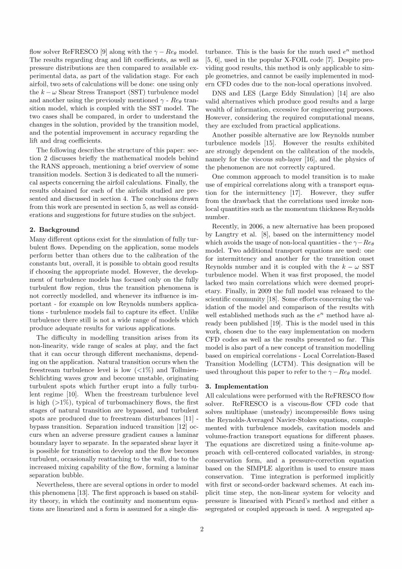
Figure 5: Transition location for the NACA 0012 airfoil,lower surface.

No case exhibits reasonable accuracy for both surfaces.It would appear that the effect of the xinlet is of higherimportance than the inlet eddy viscosity, since transitionoccurs later for conditions C. However, for the remainingangles, conditions B exhibit transition in the lower surfaceearlier than case C, while the order remains the same asbefore for the upper surface, indicating influence from thepressure gradient.

hi/h1

Cd

,f

103

0 0.5 1 1.5 26.5

7

7.5

8

8.5

= 0º - SSTp= 1.61, U= 0.54%

= 2º - SSTp= 1.56, U= 0.62%

= 4º - SSTp= 1.53, U= 0.75%

= 6º - SSTp= 1.49, U= 0.96%

= 8º - SSTp= 1.47, U= 1.3%

Figure 6: Friction drag uncertainty estimate for the NACA0012 airfoil, SST model.

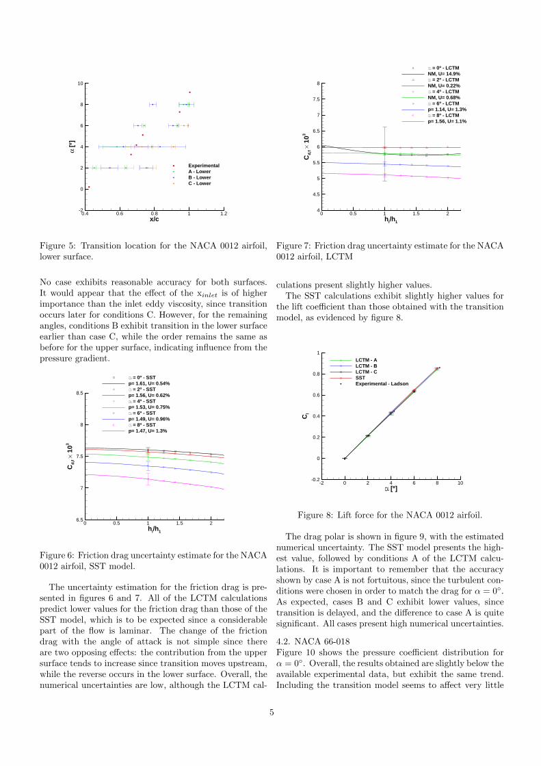
The uncertainty estimation for the friction drag is pre-sented in figures 6 and 7. All of the LCTM calculationspredict lower values for the friction drag than those of theSST model, which is to be expected since a considerablepart of the flow is laminar. The change of the frictiondrag with the angle of attack is not simple since thereare two opposing effects: the contribution from the uppersurface tends to increase since transition moves upstream,while the reverse occurs in the lower surface. Overall, thenumerical uncertainties are low, although the LCTM cal-

hi/h1

Cd

,f

103

0 0.5 1 1.5 24

4.5

5

5.5

6

6.5

7

7.5

8

= 0º - LCTMNM, U= 14.9%

= 2º - LCTMNM, U= 0.22%

= 4º - LCTMNM, U= 0.68%

= 6º - LCTMp= 1.14, U= 1.3%

= 8º - LCTMp= 1.56, U= 1.1%

Figure 7: Friction drag uncertainty estimate for the NACA0012 airfoil, LCTM

culations present slightly higher values.The SST calculations exhibit slightly higher values for

the lift coefficient than those obtained with the transitionmodel, as evidenced by figure 8.

[º]

Cl

-2 0 2 4 6 8 10-0.2

0

0.2

0.4

0.6

0.8

1

LCTM - ALCTM - BLCTM - CSSTExperimental - Ladson

Figure 8: Lift force for the NACA 0012 airfoil.

The drag polar is shown in figure 9, with the estimatednumerical uncertainty. The SST model presents the high-est value, followed by conditions A of the LCTM calcu-lations. It is important to remember that the accuracyshown by case A is not fortuitous, since the turbulent con-ditions were chosen in order to match the drag for α = 0◦.As expected, cases B and C exhibit lower values, sincetransition is delayed, and the difference to case A is quitesignificant. All cases present high numerical uncertainties.

4.2. NACA 66-018Figure 10 shows the pressure coefficient distribution forα = 0◦. Overall, the results obtained are slightly below theavailable experimental data, but exhibit the same trend.Including the transition model seems to affect very little

5

Cl

Cd ×

103

-0.2 0 0.2 0.4 0.6 0.8 14

6

8

10

12

14SSTLCTM - ALCTM - BLCTM - CExperimental - GregoryExperimental - Ladson

Figure 9: Drag force for the NACA 0012 airfoil.

the pressure coefficient.

x/c

-Cp

0 0.2 0.4 0.6 0.8 1-1

-0.5

0

0.5

1SSTLCTMExperimental

Figure 10: Pressure coefficient for the NACA 66-018 air-foil, α = 0◦.

The skin friction distribution is shown in Figure 11.Here, the differences between the SST and LCTM calcu-lations are significant: fully turbulent flow occurs in boththe upper and lower surface of the airfoil when using theSST model, as is to be expected. When the transitionmodel is used, a significant portion of the airfoil is in thelaminar regime.

The available experimental data for transition are notin accordance with the obtained results - Figure 12.

Figure 13 shows the uncertainty estimation for the fric-tion components of the drag force. The SST calculationsprovide a higher value for the friction drag, consequence ofthe fully turbulent flow condition which decreases slightlywith the increase of the angle of attack, with low uncer-tainties. Using the transition model results in lower fric-tion drag, increasing along with the angle of attack due tothe upstream movement of transition on the upper surface,

x/c

Cf

103

0 0.2 0.4 0.6 0.8 10

2

4

6

8SSTLCTM

Figure 11: Skin friction for the NACA 66-018 airfoil, α =0◦.

x/c

[º]

-0.1 0 0.1 0.2 0.3 0.4 0.5 0.6 0.7 0.8-1

0

1

2

3

4

5

6

7

Laminar Separation - ExperimentalTransition - ExperimentalTransition start - LCTMTransition end - LCTM

Figure 12: Transition location for the NACA 66-018 air-foil.

and significantly higher numerical uncertainty.

As should be expected, the drag coefficient obtainedwith the transition model is significantly lower than thatof the SST model. However, the model failed to capturethe experimental trend for the drag coefficient.

4.3. Eppler 387

4.3.1 Re = 3 × 105

Figures 15 and 16 show the pressure coefficient and skinfriction distribution for the lowest angle of attack. TheLCTM calculations exhibit a laminar separation bubble oneach side of the airfoil, which is responsible for triggeringtransition, unlike when using the SST model in which nat-ural transition always takes place. Differences in the pres-sure distribution are only found near the beginning of theadverse pressure gradient and in the separated flow zones.Regarding the lower surface, although the LCTM calcu-lations also suggest separation-induced transition, such is

6

hi/h1

0 0.5 1 1.5 23

4

5

6

7

8

9

10

= 0º - SSTp= 1.12, U= 1.31%

= 2º - SSTp= 1.11, U= 1.38%

= 3º - SSTp= 1.16, U= 1.35%

= 6º - SSTp= 1.36, U= 1.29%

Cd

,f

103

0 0.5 1 1.5 23

4

5

6

7

8

9

10

= 0º - LCTMNM, U= 5.43%

= 2º - LCTMNM, U= 16.8%

= 3º - LCTMNM, U= 1.0%

= 6º - LCTMp= 1.88, U= 0.86%

Figure 13: Uncertainty estimate for friction drag for theNACA 66-018 airfoil.

Cl

Cd

102

-0.2 0 0.2 0.4 0.6 0.80

0.5

1

1.5

2ExperimentalSSTLCTM

Figure 14: Drag for the NACA 66-018 airfoil.

x/c

-Cp

0 0.2 0.4 0.6 0.8 1-1

-0.5

0

0.5

1

1.5SST - USSST - LSLCTM - USLCTM - LSExperimental - MuellerExperimental - LTPT

Figure 15: Pressure coefficient for α = −2◦ for the Eppler387 airfoil at Re = 3 × 105.

x/c

Cf

103

0 0.2 0.4 0.6 0.8 1-10

-5

0

5

10

15SST - USSST - LSLCTM - USLCTM - LS

Figure 16: Skin friction for α = −2◦ for the Eppler 387airfoil at Re = 3 × 105.

not in accordance with the experimental data.In all cases there seems to be good agreement between

the numerical and experimental pressure coefficient distri-bution, although one set of experimental data [27] consis-tently presents slightly higher pressure in the lower sur-face. This may be due to blockage effects, since the otherset of points do not exhibit the same behaviour.

x/c

[º]

0 0.2 0.4 0.6 0.8 1-3

-2

-1

0

1

2

3

4

5

6

7

8

Laminar Separation - ExperimentalTransition - ExperimentalReattachment - ExperimentalLaminar Separation - LCTMTransition start - LCTMTransition end - LCTMReattachment - LCTM

Figure 17: Transition chordwise location for the Eppler387 airfoil at Re = 3 × 105.

Figure 17 shows the experimental and numerical loca-tion of the points of interest concerning transition and theseparated flow region, with the respective numerical uncer-tainty. A larger bubble is always obtained for the numer-ical solution. The location of laminar separation exhibitsthe smallest numerical uncertainty when compared to theother relevant points. The onset of transition as well asturbulent reattachment also exhibit a small uncertainty,while the end of transition presents the largest, a conse-quence of non-monotonic behaviour caused by the coarsestgrids.

7

hi/h1

Cd

,f

103

0 0.5 1 1.5 28

8.5

9

9.5

10

10.5

11

= 1º - LCTM

1h + 2h2, U= 2.62%

= 3º - LCTMp= 1.91, U= 0.95%

= 7º - LCTMh2, U= 0.71%

0 0.5 1 1.5 28

8.5

9

9.5

10

10.5

11

= -2º - LCTMh2, U= 0.70% = -1º - LCTMh2, U= 0.47% = 0º - LCTM

1h + 2h2, U= 2.67%

0 0.5 1 1.5 28

8.5

9

9.5

10

10.5

11

= -2º - SSTNM, U= 0.59%

= -1º - SSTp= 1.88, U= 0.49%

= 0º - SSTp= 1.86, U= 0.40%

hi/h1

Cd

,f

103

0 0.5 1 1.5 28

8.5

9

9.5

10

10.5

11

= 1º - SSTp= 1.60, U= 0.43%

= 3º - SSTp= 1.55, U= 0.46%

= 7º - SSTNM, U= 0.61%

Figure 18: Friction drag uncertainty estimate for the Ep-pler 387 airfoil at Re = 3 × 105, SST model.

0 0.5 1 1.5 24

5

6

7

= -2º - SSTNM, U= 0.59%

= -1º - SSTp= 1.88, U= 0.49%

= 0º - SSTp= 1.86, U= 0.40%

hi/h1

Cd

,f

103

0 0.5 1 1.5 24

5

6

7

= 1º - SSTp= 1.60, U= 0.43%

= 3º - SSTp= 1.55, U= 0.46%

= 7º - SSTNM, U= 0.61%

hi/h1

Cd

,f

103

0 0.5 1 1.5 24

5

6

7 = 1º - LCTM

NM, U= 2.62% = 3º - LCTM

p= 1.91, U= 0.95% = 7º - LCTM

NM, U= 0.71%

0 0.5 1 1.5 24

5

6

7

= -2º - LCTMNM, U= 0.70%

= -1º - LCTMNM, U= 0.47%

= 0º - LCTMNM, U= 2.67%

Figure 19: Friction drag uncertainty estimate for the Ep-pler 387 airfoil at Re = 3 × 105, LCTM.

The friction component of drag is presented in Figures18 and 19. The predictions obtained when using the tran-sition model are always lower than when using the SSTmodel, due to delayed transition and the appearance ofthe laminar separation bubbles. The numerical uncertain-ties are very low for both models, generally lower than1%.

The SST solutions constantly predict higher drag thanthe experimental data, a consequence of failing to capturethe laminar separation bubble - Figure 20. The values es-timated by the transition model are much closer to the ex-perimental data. In general, the transition model presentshigher uncertainties than calculations performed with theSST model, for both the lift and drag, namely the twohighest angles of attack exhibit values higher than 10%.

Cl

Cd

102

0 0.2 0.4 0.6 0.8 1 1.20

0.5

1

1.5

2

2.5

3

Experimental - LTPTLow Speed (V1)Low Speed (V3)Low Speed (V5)LCTMSST

Figure 20: Drag force for the Eppler 387 airfoil at Re =3 × 105.

x/c

-Cp

0 0.2 0.4 0.6 0.8 1

-0.5

0

0.5

SST - USSST - LSLCTM - USLCTM - LSExperimental - MuellerExperimental - LTPT

Figure 21: Pressure coefficient for α = −1◦ for the Eppler387 airfoil at Re = 1 × 105.

4.3.2 Re = 1 × 105

Figures 21 and 22 present the skin friction and pressuredistribution for the Eppler 387 airfoil at a Reynolds num-ber of 1 × 105. The pressure coefficient differs slightly inthe upper surface between the two models, both in the re-gion where a laminar separation bubble is located, as wellas in the region before it. For the lower surface, the twopressure distributions are almost overlapping. Similarlyto the previous section, the experimental pressure datashow some differences particularly in the lower surface andagain the numerical solution is more in accordance withthe LTPT data [28].

Unlike the other tested Reynolds number, the agree-ment between the experimental and numerical position oflaminar separation is not as good - figure 23. The numer-ical prediction for turbulent reattachment is also worsefor this Reynolds number. One striking consequence fromthe combined behaviour of the separation and reattach-

8

x/c

Cf

0 0.2 0.4 0.6 0.8 1

0

5

10

15

20

25

30

SST - USSST - LSLCTM - USLCTM - LS

Figure 22: Skin friction for α = −1◦ for the Eppler 387airfoil at Re = 1 × 105.

x/c

[º]

0 0.2 0.4 0.6 0.8 1

-2

-1

0

1

2

3

4

5

6

7

8

9

Laminar Separation - ExpTransition - ExpReattachment - ExpLaminar Separation - NumTransition start - NumReattach - Num

Figure 23: Transition chordwise location for the Eppler387 airfoil at Re = 1 × 105.

ment locations is in the size of the bubble: the numericalsolution always exhibits a larger separated region than thewind-tunnel data, particularly for the higher angles.

The total drag obtained from the SST model is muchlower than both experimental data and transition modelcalculations - Figure 24. The latter matches well with theformer for the lower angles, but clearly overpredicts thedrag for the higher angles when the effect of the bubbleshould be decreasing. Much like before, the numerical un-certainty is higher for the LCTM case and a clear growthis seen when increasing the angle of attack. This suggeststhe grids are not fine enough for these angles, as monotonicconvergence was obtained for these cases.

5. ConclusionsIn this thesis the effect of transition modelling on the flowfor three different airfoils was analyzed. The γ−Reθ tran-sition model of Langtry and Menter was used and the re-sults were compared with baseline calculations using only

Cl

Cd

102

0 0.2 0.4 0.6 0.8 1 1.20

0.5

1

1.5

2

2.5

3

3.5

4LTPTLow Speed (V1)Low Speed (V3)Low Speed (V5)SSTLCTM

(b) Drag Polar

Figure 24: Drag force for the Eppler 387 airfoil at Re =1 × 105.

the SST k−ω turbulence model and available experimen-tal data. The three airfoils tested were the NACA 0012,NACA 66-018 and the Eppler 387 airfoil.

The work performed provided the following conclusions:

• The main work showed that the transition modelis not as numerically robust as the SST turbulencemodel: iterative convergence becomes much more dif-ficult.

• The transition model is much more sensitive to theinlet turbulence settings, namely the eddy viscosity,unlike the SST model. This higher sensitivity is ag-gravated by the turbulent decay that is greatly over-estimated by common turbulence models, meaningthat information regarding turbulence should also beprovided in experimental testing, in order to extractproper conclusions regarding model validation.

• The uncertainty estimation for the pressure and fric-tion components of drag and lift showed that higherdiscretization errors are obtained when the γ − Reθmodel is used and can reach extremely high valuesin some cases. Transition can occur at regions wherethe grid is not sufficiently refined in the streamwisedirection, causing non-monotonic behaviour.

• The calculations on the Eppler 387 airfoil showed thatthe transition model correctly predicted laminar sep-aration but causes reattachment to occur too late.Separation induced transition is the case that showsthe best iterative convergence properties.

• On the contrary, cases where natural transition is ex-pected, such as in the NACA 0012 airfoil, are highlydependent on the combination of turbulence bound-ary conditions and turbulence decay.

9

• Overall, the calculations with the transition modelshowed an improvement in accuracy when comparedto the SST solutions. The skin friction curves showedclear differences, but a clear comparison is not evi-dent since no experimental data was available. Thelift coefficient suffered little change, while the dragshowed a clear improvement for most cases.

Future work on this topic should include a more detailedstudy on the effect of the inlet turbulent variables, as theirspecification seems to have a major impact on the solution.This is valid not only for cases where natural transitiontakes place, but also for geometries were laminar separa-tion bubbles are formed. It would be interesting to com-pare the γ−Reθ model with other available alternatives fortransition modelling, or even implementations with otherturbulence models. Finally, the behaviour of the model inthree-dimensional problems is also worthy of some atten-tion, given the higher complexity of the boundary layer inthese situations.

References[1] J. H. Ferziger and M. Peric. Computational methods for fluid

dynamics. 3rd Ed., Springer, 2012.

[2] T. J. Mueller and J. D. DeLaurier. Aerodynamics of small ve-hicles. Annual Review of Fluid Mechanics, 35(1):89–111, 2003.

[3] T. J. Mueller. Low Reynolds number vehicles. Technical report,DTIC Document, 1985.

[4] W. Shyy, Y. Lian, J. Tang, D. Viieru, and H. Liu. Aerody-namics of low Reynolds number flyers, volume 22. CambridgeUniversity Press, 2007.

[5] A. M. O. Smith and N. Gamberoni. Transition, pressure gradi-ent and stability theory. Douglas Aircraft Company, El SegundoDivision, 1956.

[6] J. L. Van Ingen. A suggested semi-empirical method for thecalculation of the boundary layer transition region. Technicalreport, Delft University of Technology, 1956.

[7] M. Drela and M. B. Giles. Viscous-inviscid analysis of transonicand low Reynolds number airfoils. AIAA journal, 25(10):1347–1355, 1987.

[8] F. R. Menter, R. B. Langtry, S. R. Likki, Y. B. Suzen, P. G.Huang, and S. Volker. A correlation-based transition modelusing local variablespart i: model formulation. Journal of tur-bomachinery, 128(3):413–422, 2006.

[9] ReFRESCO, 2015. URL http://www.refresco.org.

[10] H. Schlichting and K. Gersten. Boundary-layer theory.Springer, 2000.

[11] M. V. Morkovin. On the many faces of transition. In Viscousdrag reduction, pages 1–31. Springer, 1969.

[12] R. E. Mayle. The role of laminar-turbulent transition in gasturbine engines. Journal of Turbomachinery, 113(4):509–536,1991.

[13] D. D. Pasquale, A. Rona, and S. J. Garrett. A selective re-view of CFD transition models. 39th AIAA Fluid DynamicsConference, 2009, San Antonio, Texas, American Institute ofAeronautics and Astronautics, June 2009.

[14] R. G. Jacobs and P. A. Durbin. Simulations of bypass transi-tion. Journal of Fluid Mechanics, 428:185–212, 2001.

[15] D. C. Wilcox. Turbulence Modeling for CFD. 2nd Edition,DCW Industries, Inc., 2004.

[16] A. M. Savill. Some recent progress in the turbulence modellingof bypass transition. Near-wall turbulent flows, pages 829–848,1993.

[17] J. Steelant and E. Dick. Modelling of bypass transition withconditioned Navier-Stokes equations coupled to an intermit-tency transport equation. International journal for numericalmethods in fluids, 23(3):193–220, 1996.

[18] R. B. Langtry and F. R. Menter. Correlation-based transitionmodeling for unstructured parallelized computational fluid dy-namics codes. AIAA journal, 47(12):2894–2906, 2009.

[19] C. Seyfert and A. Krumbein. Evaluation of a correlation-basedtransition model and comparison with the en method. Journalof Aircraft, 49(6):1765–1773, 2012.

[20] L. Eca. Grid generation tools for structured grids. TechnicalReport Report D72-18, Instituto Superior Tecnico, 2003.

[21] R. B. Langtry. A correlation-based transition model using localvariables for unstructured parallelized CFD codes. PhD thesis,Universitat Stuttgart, 2006.

[22] L. Eca and M. Hoekstra. A procedure for the estimation ofthe numerical uncertainty of CFD calculations based on gridrefinement studies. Journal of Computational Physics, 262:104–130, 2014.

[23] P. R. Spalart and C. L. Rumsey. Effective inflow conditions forturbulence models in aerodynamic calculations. AIAA journal,45(10):2544–2553, 2007.

[24] N. Gregory and C. L. OReilly. Low-speed aerodynamic char-acteristics of NACA 0012 aerofoil section, including the effectsof upper-surface roughness simulating hoar frost. Technical re-port, 1970.

[25] C. Ladson. Effects of independent variation of Mach andReynolds numbers on the low-speed aerodynamic characteris-tics of the NACA 0012 airfoil section. Technical report, 1988.

[26] D. E. Gault. An experimental investigation of regions of sepa-rated laminar flow. Number 3505. National Advisory Commit-tee for Aeronautics, 1955.

[27] G. M. Cole and T. J. Mueller. Experimental measurements ofthe laminar separation bubble on an Eppler 387 airfoil at lowReynolds numbers. NASA STI/Recon Technical Report N, 90:15380, 1990.

[28] R. J. Mcghee, B. S. Walker, and B. F. Millard. Experimentalresults for the Eppler 387 airfoil at low Reynolds numbers inthe Langley low-turbulence pressure tunnel. 1988.

[29] M. S. Selig, J. J. Guglielmo, A. P. Broeren, and Gigure P. Sum-mary of low speed airfoil data, volume 1. SoarTech, 1995.

[30] M. S. Selig, C. A. Lyon, A. P. Broeren, Gigure P., andGopalarathnam A. Summary of low speed airfoil data, vol-ume 3. SoarTech, 1997.

[31] G. A. Williamson, B. D. McGranahan, B. A. Broughton, R. W.Deters, J. B. Brandt, and M. S. Selig. Summary of low speedairfoil data, volume 5. SoarTech, 2012.

[32] R. M. A. Lopes. Calculation of the flow around hydrofoils atmoderate Reynolds numbers. Master’s thesis, Instituto Supe-rior Tecnico, 2015.

10