Calculations in Chemistry

Dr. S. Sri Skandaraja

Department of ChemistryUniversity of Kelaniya

CHEM 11111

Graphical presentation of data

Straight line graphs

How variable „y‟ changes as variable „x‟

changes

y = mx + c where m =slope

c= intercept

Tables and graphs are visual representations. They are used to

organise information to show patterns and relationships. A graph

shows this information by representing it as a shape.

line graphs

Displaying Qualitative Data

“Sometimes you can see a lot just

by looking.”

Absorption of light by matter

the Beer Lambert law

A = ecl

A = -log T = - log I/Io

T=I/Io = 10-ecl

Concentration

Ab

so

rba

nc

e, A

Slope = el

Absorbance & concentration

A = ecly = mx

0

0.5

1

Concentration

Tra

ns

mit

tan

ce

, T

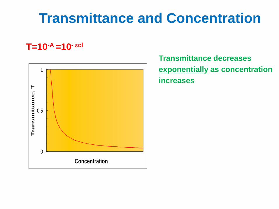
Transmittance decreases

exponentially as concentration

increases

T=10-A =10- ecl

Transmittance and Concentration

First order

ln[A] =-kt +ln[A0]

[A] = [A0]e-kt

kinetics

Second order

Zeroth order

[A] =-kt +[A0]

Calibration Techniques

1. Calibration Curve Method

2. Standard Additions Method

3. Internal Standard Method

Calibration Curve Method

1. Most convenient when a large number

of similar samples are to be analyzed.

2. Most common technique.

Calibration Curve Procedure

1. Prepare a series of standard solutions

(analyte solutions with known

concentrations).

2. Plot [analyte] vs. Analytical Signal.

3. Use signal for unknown to find [analyte].

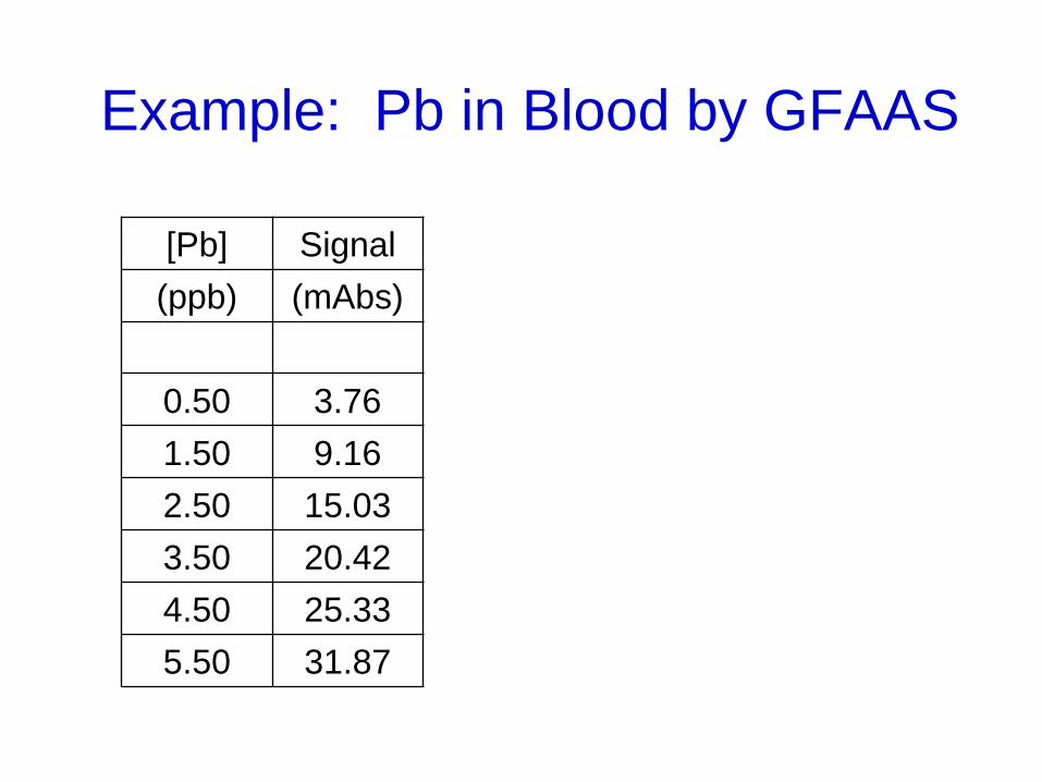
Example: Pb in Blood by GFAAS

[Pb] Signal

(ppb) (mAbs)

0.50 3.76

1.50 9.16

2.50 15.03

3.50 20.42

4.50 25.33

5.50 31.87

0

5

10

15

20

25

30

35

0 1 2 3 4 5 6

Pb Concentration (ppb)

mA

bs

y = 5.56x + 0.93

Example: Pb in Blood by GFAAS

[Pb] Signal

(ppb) (mAbs)

0.50 3.76

1.50 9.16

2.50 15.03

3.50 20.42

4.50 25.33

5.50 31.87

Results of linear regression:

S = mC + b

m = 5.56 mAbs/ppb

b = 0.93 mAbs

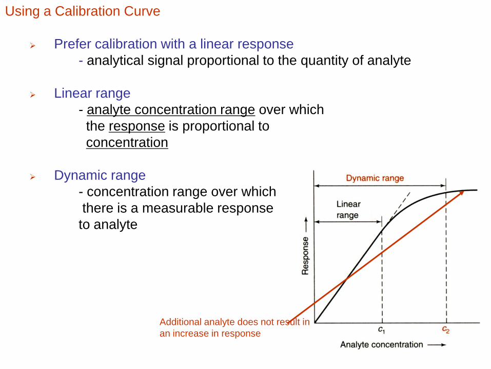
Using a Calibration Curve

Prefer calibration with a linear response

- analytical signal proportional to the quantity of analyte

Linear range

- analyte concentration range over which

the response is proportional to

concentration

Dynamic range

- concentration range over which

there is a measurable response

to analyte

Additional analyte does not result in

an increase in response

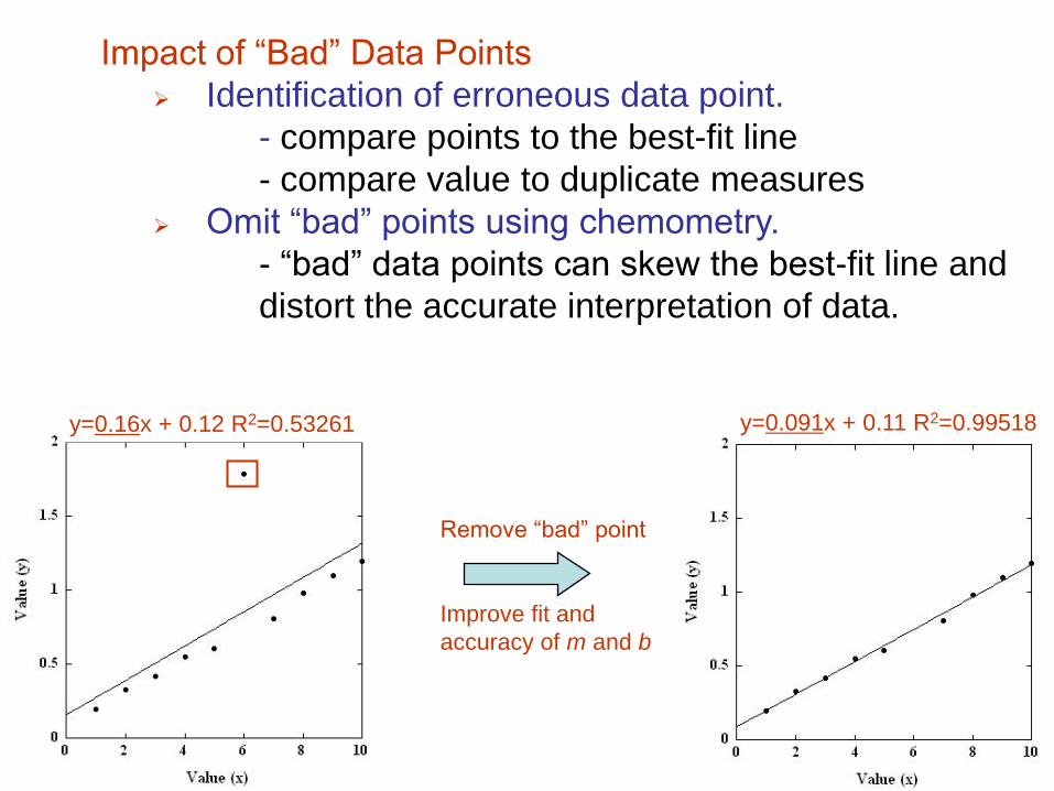
Impact of “Bad” Data Points

Identification of erroneous data point.

- compare points to the best-fit line

- compare value to duplicate measures

Omit “bad” points using chemometry.

- “bad” data points can skew the best-fit line and

distort the accurate interpretation of data.

Remove “bad” point

Improve fit and

accuracy of m and b

y=0.16x + 0.12 R2=0.53261 y=0.091x + 0.11 R2=0.99518

Limitations in a Calibration Curve

(iv)Limited application of calibration curve to

determine an unknown.

- Limited to linear range of curve

- Limited to range of experimentally determined

response for known

analyte concentrations

Unreliable determination

of analyte concentration

Uncertainty increases further

from experimental points

The product-moment correlation coefficient

The first problem - is the calibration plot linear?

A common method of estimating how well the experimental points fit a straight line is to calculate the product-moment correlation coefficient, r.

This statistic is often referred to simply as the ‘correlation coefficient’

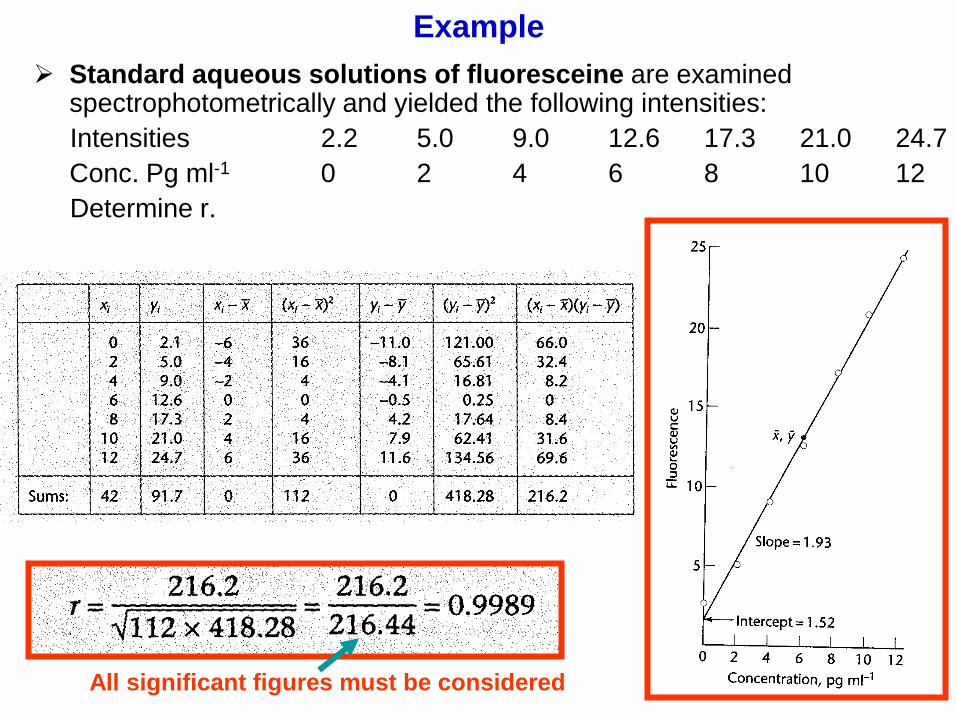
Example

Standard aqueous solutions of fluoresceine are examined spectrophotometrically and yielded the following intensities:

Intensities 2.2 5.0 9.0 12.6 17.3 21.0 24.7

Conc. Pg ml-1 0 2 4 6 8 10 12

Determine r.

All significant figures must be considered

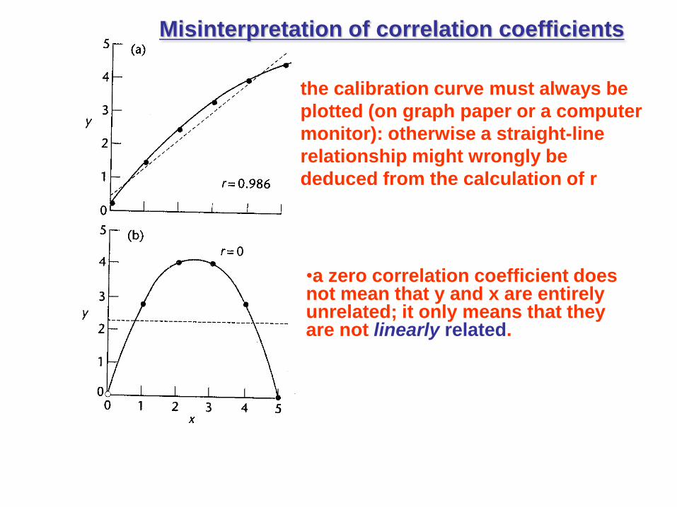
the calibration curve must always be

plotted (on graph paper or a computer

monitor): otherwise a straight-line

relationship might wrongly be

deduced from the calculation of r

•a zero correlation coefficient does not mean that y and x are entirely unrelated; it only means that they are not linearly related.

Misinterpretation of correlation coefficients

Standard Addition In standard addition, known quantities of analyte are

added to the unknown.

From the increase in signal, we deduce how much

analyte was in the original unknown.

This method requires a linear response to analyte.

Standard addition is especially appropriate when the

sample composition is unknown or complex and

affects the analytical signal.

The matrix is everything in the unknown, other than

analyte.

A matrix effect is a change in the analytical signal

caused by anything in the sample other than analyte.

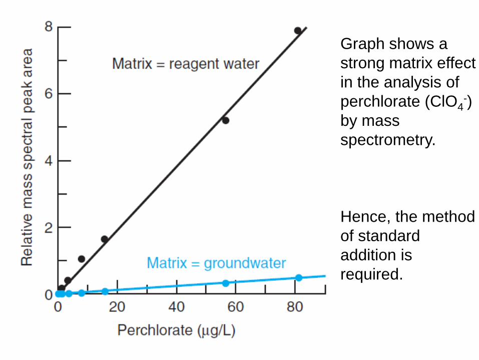
Graph shows a

strong matrix effect

in the analysis of

perchlorate (ClO4-)

by mass

spectrometry.

Hence, the method

of standard

addition is

required.

Consider a standard addition in which a sample

with unknown initial concentration of analyte [X]igives a signal intensity IX.

Then a known concentration of standard, S, is

added to an aliquot of the sample and a signal ISX is

observed for this second solution.

Addition of standard to the unknown changes the

concentration of the original analyte because of

dilution.

Diluted concentration of analyte = [X]f;

Where “f” stands for “final.”

Concentration of standard in the final solution = [S]f. (Bear in mind that the chemical species X and S are the same.)

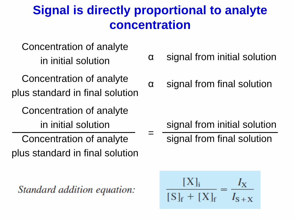
Signal is directly proportional to analyte

concentration

Concentration of analyte

in initial solution

Concentration of analyte

plus standard in final solution

signal from initial solution

signal from final solution=

Concentration of analyte

in initial solution signal from initial solutionα

Concentration of analyte

plus standard in final solutionsignal from final solutionα

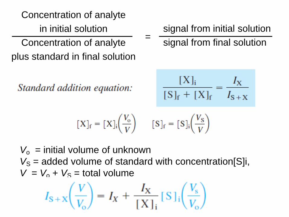
Concentration of analyte

in initial solution

Concentration of analyte

plus standard in final solution

signal from initial solution

signal from final solution=

Vo = initial volume of unknown

VS = added volume of standard with concentration[S]i,

V = Vo + VS = total volume

Serum containing Sodium gave a signal of 4.27 mV in an

atomic emission analysis. Then 5.00 mL of 2.08 M NaCl

were added to 95.0 mL of serum. This spiked serum gave

a signal of 7.98 mV. Find the original concentration of

Sodium in the serum.

Graphical Procedure for Standard

Addition

There are two common methods to perform standard

addition.

If the analysis does not consume solution, we begin with

an unknown solution and measure the analytical signal.

Then, we add a small volume of concentrated standard

and measure the signal again.

We add several more small volumes of standard and

measure the signal after each addition.

Standard should be concentrated so that only small volumes

are added and the sample matrix is not appreciably altered.

Added standards should increase the analytical signal by a

factor of 1.5 to 3.

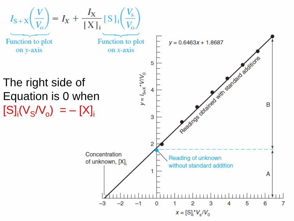
The right side of

Equation is 0 when

[S]i(VS/Vo) = – [X]i