Calibration of Laser Induced Fluorescence Thermometry Using 2'7

OREGON STATE UNIVERSITY

Calibration of Laser Induced Fluorescence

Thermometry Using 2'7' Dichlorofluorescein

and Sulforhodamine B PH 403 Senior Thesis

With Dr. Vinod Narayanan

Jaryd Ulbricht

5/30/2012

Jaryd Ulbricht May 30, 2012

1

Contents

Table of Figures ............................................................................................................................................ 2

Index of Equations ........................................................................................................................................ 3

Abstract ......................................................................................................................................................... 4

Introduction ................................................................................................................................................... 4

Laser Induced Fluorescence ...................................................................................................................... 4

Two Dye Two Color Method .................................................................................................................... 5

Experimental Dyes .................................................................................................................................... 5

2'7' Dichlorofluorescein (C20H10Cl2O5) ................................................................................................. 6

Sulforhodamine B (C27H30N2O7S2) ....................................................................................................... 6

Methods ........................................................................................................................................................ 9

Experimental Set Up ................................................................................................................................. 9

Determining Dye Concentrations............................................................................................................ 12

Results ......................................................................................................................................................... 15

Analysis ...................................................................................................................................................... 19

Dye Concentration Error ......................................................................................................................... 19

Determining Calibration Curve ............................................................................................................... 20

Conclusions ................................................................................................................................................. 20

Acknowledgements ..................................................................................................................................... 22

Works Cited ................................................................................................................................................ 23


2

Table of Figures

Figure 1: Emission spectra of FL27 and SRhB. ............................................................................. 8

Figure 2: Solid model of experimental design ................................................................................ 9

Figure 3: Stereoscopic Lens without filter attachment ................................................................. 10

Figure 4: Stereoscopic Lens and camera with filter attachment. On the right is the bandpass filter

and on the left is the high pass filter ............................................................................................. 10

Figure 5: Registration Calibration Image ..................................................................................... 11

Figure 6: Camera image of both dyes (FL27 left and SRhB right) at 24 ° C ............................... 11

Figure 7: Camera image of both dyes (FL27 left and SRhB right) at 65° C ................................ 12

Figure 8: pH dependency of dyes. The intensity spike at 532 nm is from a Nd:YAG laser

captured by the camera ................................................................................................................. 13

Figure 9: Early experimental data depicting the intensity ratio as a function of temperature ...... 14

Figure 10: SRhB and FL27 Absorption Spectrum ........................................................................ 14

Figure 11: FL27 intensity dependence on SRhB concentration ................................................... 15

Figure 12: Intensity of SRhB showing low resolution ................................................................. 16

Figure 13: Initial Calibration ........................................................................................................ 17

Figure 14: Final Calibration .......................................................................................................... 18

Figure 15: Experimental results and deviation from theoretical model ........................................ 19

Figure 16: Experimental Results ................................................................................................... 20


3

Index of Equations

Equation 1. ...................................................................................................................................... 4

Equation 2 ....................................................................................................................................... 5

Equation 3 ....................................................................................................................................... 5

Equation 4 ....................................................................................................................................... 5

Equation 5 ....................................................................................................................................... 5

Equation 6 ...................................................................................................................................... 7

Equation 7 ...................................................................................................................................... 7

Equation 8 ...................................................................................................................................... 7

Equation 9 ...................................................................................................................................... 7

Equation 10 .................................................................................................................................. 18

Equation 11 .................................................................................................................................. 18

Equation 12 .................................................................................................................................. 19


4

Abstract

An apparatus and method for calibrating planar laser induced fluorescence using a two-dye, two-

color method was developed. A laser sheet was expanded from a 473 nm laser to excite dye

solutions into higher energy states then fluoresced through spontaneous emission. The two

fluorescent dyes selected for research and development were the primarily green emitting 2'7'

dichlorofluorescein and the primarily red emitting sulforhodamine B. Planar laser induced

fluorescence is used in thermal-fluids experiments as an accurate, non-invasive method for

developing flow thermographs used to characterize the performance of experimental devices and

methods. Two-color, two-dye methods are used because of their high accuracy, and potentially

higher sensitivity relative to other thermography techniques because the temperature can be

expressed as a function of only the fluorescence ratio of the two dyes and is independent of local

laser intensity, which may vary considerably with time and space during an experiment.

Calibration curves and relationships were developed that accurately correlated the local

temperature of the solution to the intensity ratio of the dyes. Using a concentration of 2'7'

Dichlorofluorescein of and a concentration of Sulforhodamine B of

predicted temperature measurements had an uncertainty of 2.09 °C.

Introduction

Laser Induced Fluorescence

Laser-induced fluorescence (LIF) has provided an accurate and especially useful tool in the

analysis of fluid flows and thermodynamics. Conventional methods of measuring temperature

within a liquid by use of thermocouples and other intrusive measuring devices have proven

unreliable as the physical presence of the temperature measuring device inhibits fluid flow. LIF

has provided a non-intrusive method of temperature measurement that allows the characteristics

of the flow to be unaffected as well as being able to define the temperature at any local point in a

planar sheet of the liquid. In order to utilize an LIF system, temperature/intensity curves must be

determined in order to calibrate the measuring device.

In this paper, the process of calibrating an LIF system will be explained in detail including the

determination of optimum dye concentration ratios, construction of a calibration apparatus, and

testing of such an apparatus.

There has been no small amount of research on LIF thermometry, but little has been done to

document the calibration process. Proper concentrations of dye are critical to the success of any

LIF process as well as the design of a proper calibration system. It is essential then to record this

procedure for future use.

The irradiated intensity of the fluorescent dyes can be modeled by the following equation

(Guilbault, 1990):

𝑰 = 𝑰𝟎𝛃𝐜𝚽(𝟏 − 𝒆 𝜺𝒃𝑪) 1

where I0 is the intensity of the laser, β0 is the collection efficiency, Φ is the quantum efficiency, ε

is the molar absorptivity, b is the absorption path length and C is the concentration of the dye. If

the argument of the exponent is small (e.g. <<1) than


5

=∑

=

−

𝒂𝒏𝒅 𝑰 𝑰𝟎𝛃𝐜𝚽𝜺𝒃𝑪

And the intensity can be seen to be linear in regards to all the explicit parameters.

2

Two Dye Two Color Method

In order to accurately measure the temperature of the dye solution the fluorescent intensity must

be normalized to the intensity of the laser light. This is a difficult and tedious task, but if two

dyes are used and their intensities are measured simultaneously then the relative signals will both

depend on the same optical path length and incident laser beam intensity. Therefore normalizing

the dye fluorescence to the laser is no longer necessary if two dyes, Dye A and Dye B, are

prepared in a single sample.

𝑰𝑨 = 𝑰𝟎𝛃𝐀𝐜𝚽𝐀𝜺𝑨𝒃𝑪𝑨

3

𝑰𝑩 = 𝑰𝟎𝛃𝐁𝐜𝚽𝐁𝜺𝑩𝒃𝑪𝑩

4

IA and IB are the intensities of each dye. When dividing both intensity measurements by each

other

𝑰𝑨𝑰𝑩=𝛃𝐜𝐀𝚽𝐀𝜺𝑨𝑪𝑨𝛃𝐜𝐁𝚽𝐁𝜺𝑩𝑪𝑩

5

The incident laser sheet intensity and absorption path length, I0 and b respectively, drop out and

their relative intensities will be constant even if the lasers intensity is not. Measuring the signal

from the two dyes also allows us to make measurements deep into the sample and not have to

account for the absorption (and therefore decreased absolute intensity) of the laser light.

Experimental Dyes

2'7' Dichlorofluorescein (FL27) and Sulforhodamine B (SRhB) are the dyes being explored in

this paper. Much previous work in LIF has used two dyes, one whose quantum efficiency varies

linearly with temperature and one that remains constant. In contrast, by using two dyes whose

temperature dependence is inversely related to each other (the quantum efficiency of FL27

increases linearly with temperature while the quantum efficiency of SRhB decreases with

temperature) changes in temperature can be more accurately measured, decreasing the

uncertainty in the results.


6

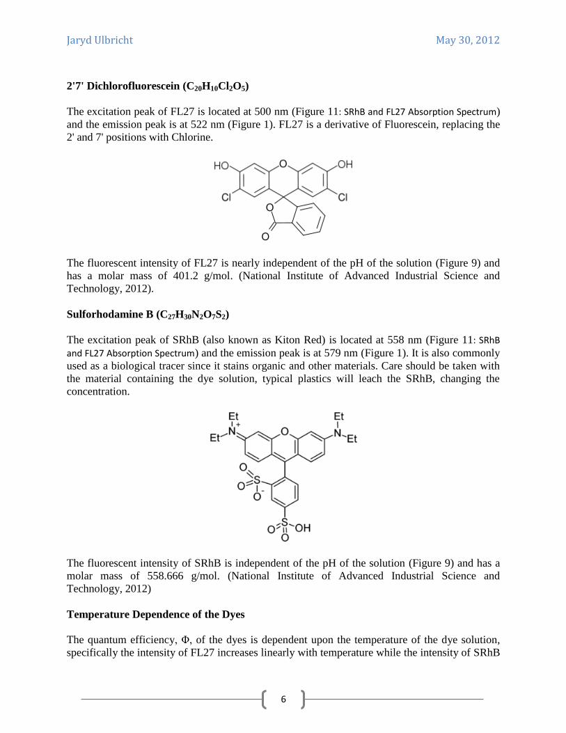
2'7' Dichlorofluorescein (C20H10Cl2O5)

The excitation peak of FL27 is located at 500 nm (Figure 11: SRhB and FL27 Absorption Spectrum)

and the emission peak is at 522 nm (Figure 1). FL27 is a derivative of Fluorescein, replacing the

2' and 7' positions with Chlorine.

The fluorescent intensity of FL27 is nearly independent of the pH of the solution (Figure 9) and

has a molar mass of 401.2 g/mol. (National Institute of Advanced Industrial Science and

Technology, 2012).

Sulforhodamine B (C27H30N2O7S2)

The excitation peak of SRhB (also known as Kiton Red) is located at 558 nm (Figure 11: SRhB

and FL27 Absorption Spectrum) and the emission peak is at 579 nm (Figure 1). It is also commonly

used as a biological tracer since it stains organic and other materials. Care should be taken with

the material containing the dye solution, typical plastics will leach the SRhB, changing the

concentration.

The fluorescent intensity of SRhB is independent of the pH of the solution (Figure 9) and has a

molar mass of 558.666 g/mol. (National Institute of Advanced Industrial Science and

Technology, 2012)

Temperature Dependence of the Dyes

The quantum efficiency, Φ, of the dyes is dependent upon the temperature of the dye solution,

specifically the intensity of FL27 increases linearly with temperature while the intensity of SRhB


7

decreases linearly with temperature at about -2.6% K-1

(V K Natrajan, 2008). By manipulating

the relationship between the intensities of each dye and modeling the quantum efficiency as

𝜱𝑨(𝑻) = 𝒂𝑻 𝒃

𝜱𝑩(𝑻) = 𝒅 − 𝒄𝑻

T being the temperature while a, b, c and d are constants. A relationship between temperature

and relative intensity can be found by substituting the quantum efficiency into the equation

= (

)

− =

6

IAB represents the relative fluorescent intensity measurement of the dyes. The term in parenthesis

is invariant with temperature and can therefore be treated as an arbitrary constant for calibration

purposes and absorbed into the quantum efficiency.

= ( )

− =

−

7

Solving for temperature (T) yields

=

( −

)

8

The constants are arbitrary and are picked to fit the temperature/intensity curve, so we do away

with the fractions and retain only three constants.

𝑻 = 𝚨(𝑰𝑨𝑩 − 𝚩

𝚪 𝑰𝑨𝑩)

9

Figure 1 shows the emission spectra of both FL27 and SRhB as a function of wavelength using a

fluorometer to measure the fluorescent intensity. The large spike at 532 nm is residual laser light

captured from a Nd:YAG 532 nm laser used to excite the dyes (see Methods: Determining Dye

Concentration). A band-pass filter (dashed purple line) excludes the emissions of SRhB and a

high-pass filter (dashed orange line) excludes emissions from FL27. The dyes emission peaks are

at two distinct wavelengths, hence this two dye method is also commonly referred to as ‘two

color’ LIF.


8

Figure 1: Emission spectra of FL27 and SRhB.

0

0.1

0.2

0.3

0.4

0.5

0.6

0.7

0.8

0.9

1

470 490 510 530 550 570 590 610 630 650 670

NO

RM

_EM

ISSI

ON

WaveLenght (nm)

EMISSION SPECTRA

FL27

SRhB

FL27+SRhB

Band Pass Filter

High Pass Filter


9

Methods

Experimental Set Up

Figure 2: Solid model of experimental design

A cylindrical lens was used to create a planar laser sheet on one side of the test cell from a Sintec

Optronics DPSS laser mounted on aluminum railing. The CCD high-speed camera was mounted

with a macro stereoscopic lens used for viewing two near-identical images with a single camera.

A high-pass filter (561 nm) and a band-pass filter (525-545 nm) were attached to the front of the

stereoscopic lens each covering one aperture.

High speed camera

473 nm Laser

Test Cell containing dye

solution

Graham

Condenser


10

Figure 5: Lens and filter array diagram

The lens was focused on the laser sheet in the test cell as shown in Figure 5. The stereoscopic

lens places two near identical images on the camera objective, each image being separately

filtered for each dye. In Figure 7 and Figure 8 the filtering of the images can clearly be seen at 24

°C and 65 °C respectively. Each half of the image is actually identical, just filtered for different

wavelengths. This method of resolving the desired wavelengths absolves us of the need of

needing two cameras to image both dye emissions simultaneously.

To account for the shift in images from the stereoscopic lens, a transformation script was written

into an analysis program which calibrated the images by comparing them to a checkered

Figure 4: Stereoscopic Lens and camera

with filter attachment. On the right is the

bandpass filter and on the left is the high

pass filter

Figure 3: Stereoscopic Lens without

filter attachment


11

background before testing began (Figure 6). The bandpass filter passed fewer wavelengths than

the highpass filter, as a result the intensity was decreased on that half of the image and had to be

accounted for when determining dye concentrations.

The camera viewed the cell oriented orthogonal to the laser path and normal to the surface of the

cell to reduce imaging refracted laser light. The entire apparatus (laser, camera and test cell) was

mounted on a single aluminum frame for ease of use.

Figure 7: Camera image of both dyes (FL27 left and SRhB right) at 24 ° C

Figure 6: Registration Calibration Image


12

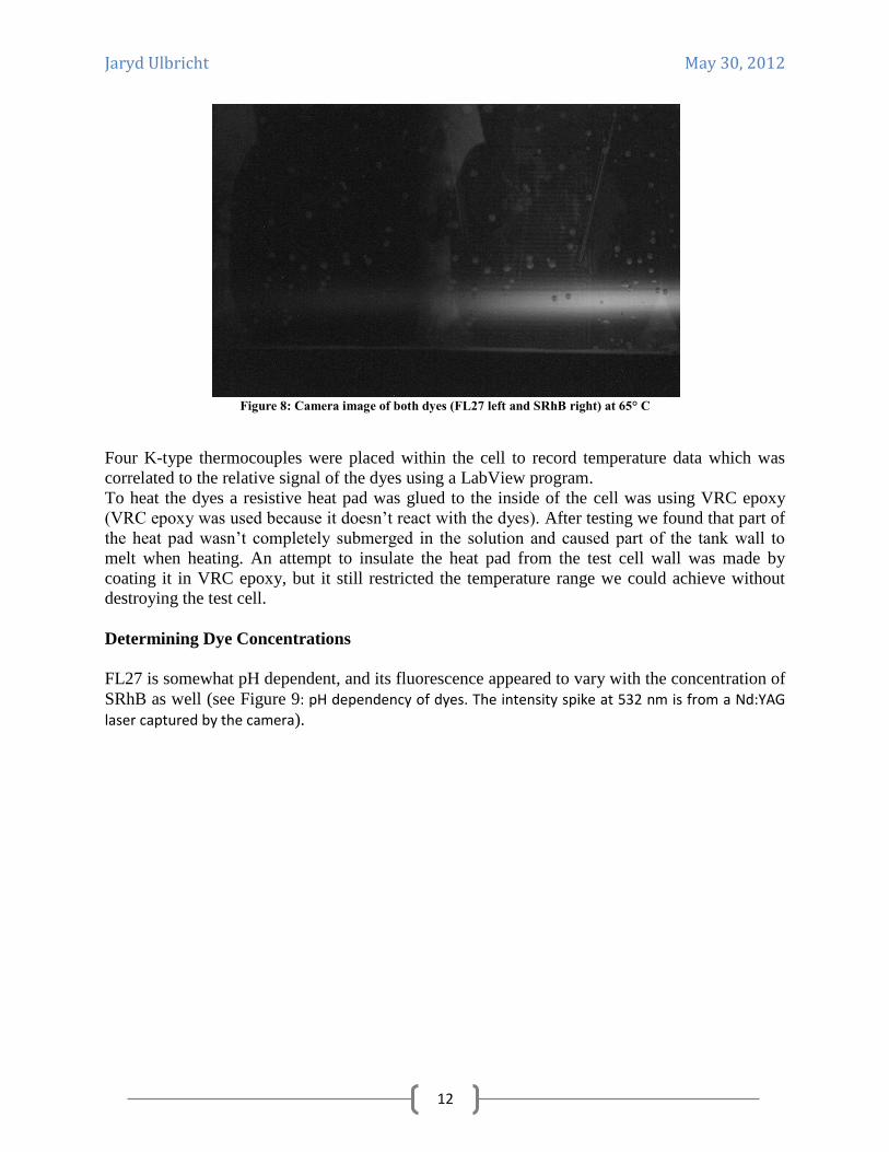
Figure 8: Camera image of both dyes (FL27 left and SRhB right) at 65° C

Four K-type thermocouples were placed within the cell to record temperature data which was

correlated to the relative signal of the dyes using a LabView program.

To heat the dyes a resistive heat pad was glued to the inside of the cell was using VRC epoxy

(VRC epoxy was used because it doesn’t react with the dyes). After testing we found that part of

the heat pad wasn’t completely submerged in the solution and caused part of the tank wall to

melt when heating. An attempt to insulate the heat pad from the test cell wall was made by

coating it in VRC epoxy, but it still restricted the temperature range we could achieve without

destroying the test cell.

Determining Dye Concentrations

FL27 is somewhat pH dependent, and its fluorescence appeared to vary with the concentration of

SRhB as well (see Figure 9: pH dependency of dyes. The intensity spike at 532 nm is from a Nd:YAG

laser captured by the camera).


13

Figure 9: pH dependency of dyes. The intensity spike at 532 nm is from a Nd:YAG laser captured by the camera

It was therefore very important to eliminate any variation in concentration during the testing

procedures. One of the causes of concentration discrepancy was evaporation of water from the

solution as it was heated. To reduce this effect a Graham condenser was affixed to the top of the

test cell. This returned the water to the sample quickly enough that the volume of the solution

remained stable during the testing and also opened the cell to atmospheric pressure reducing any

pressure dependent variables in the intensity.

The dye solution was heated from 24° C to 90 ° C and allowed to reach a steady state at several

temperatures while the camera captured images. To ensure even heating a stir rod attached to a

motor was suspended above the test cell and ran during the entire test. Nine points were plotted

during the test of the relative intensities of dyes and then graphed against the temperature of the

test cell.

0

500

1000

1500

2000

2500

3000

3500

4000

4500

450 470 490 510 530 550 570 590 610 630 650 670 690

Inte

nsi

ty (

arb

itra

y u

nit

s)

Wavelength (nm)

pH Dependency of FL27 and SRhB

FL27+SRhB pH~7

FL27+SRhB pH~11


14

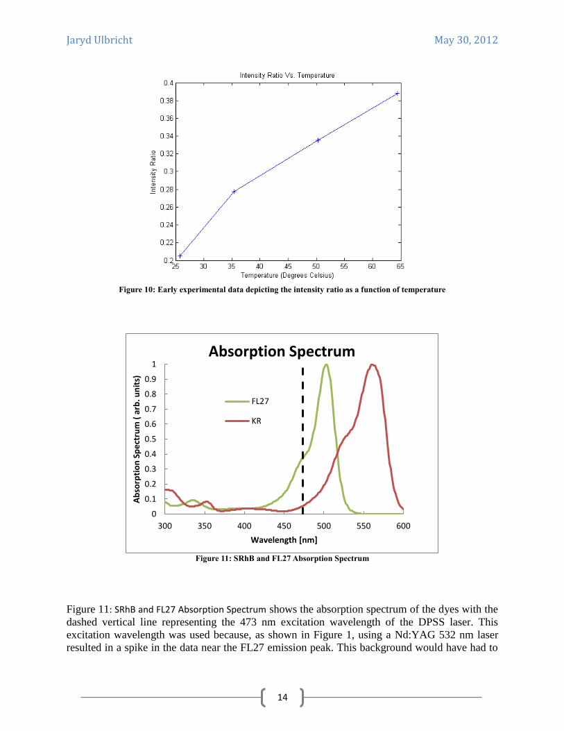
Figure 10: Early experimental data depicting the intensity ratio as a function of temperature

Figure 11: SRhB and FL27 Absorption Spectrum

Figure 11: SRhB and FL27 Absorption Spectrum shows the absorption spectrum of the dyes with the

dashed vertical line representing the 473 nm excitation wavelength of the DPSS laser. This

excitation wavelength was used because, as shown in Figure 1, using a Nd:YAG 532 nm laser

resulted in a spike in the data near the FL27 emission peak. This background would have had to

0

0.1

0.2

0.3

0.4

0.5

0.6

0.7

0.8

0.9

1

300 350 400 450 500 550 600

Ab

sorp

tio

n S

pe

ctru

m (

arb

. un

its)

Wavelength [nm]

Absorption Spectrum

FL27

KR


15

been removed by the use of a notch filter in order to get accurate results. Rather, a 473 nm

excitation wavelength was used, which was still within the absorption range of both FL27 and

SRhB.

To determine the most efficient dye concentration a fluorometer was employed. Multiple

samples were prepared using a high concentration of dye then diluting them down several orders

of magnitude using deionized (DI) water. The two dyes were mixed and measured

simultaneously since they appeared react with each other and exhibited unpredicted behavior.

The fluorometer was able to both scan the emission spectrum of the dyes and provide relative

intensity readings at specific wavelengths. The excitation wavelength was set to 473 nm with a

2.5 nm slit width using a xenon bulb. 4 mL cuvettes containing the dye solution were inserted

into the fluorometer. For each sample 5 intensities were recorded and then averaged at 585±2.5

nm and also 520±2.5 nm in order to record data at both emission peaks. The fluorometer

integrated for one second before displaying a measure of the intensity at each wavelength.

Since SRhB decreases intensity with temperature and FL27 increases both dyes must emit at

nearly the same amplitude and at least a few orders of magnitude above background readings to

help eliminate error in the measurements.

Results

Preliminary testing showed that the intensity of FL27 depended very much on the concentration

of SRhB. Much care was therefore taken in determining the final concentration of the dye

solution.

Figure 12: FL27 intensity dependence on SRhB concentration

0

20

40

60

80

100

120

140

160

180

0.00E+00 5.00E-07 1.00E-06 1.50E-06

Inte

nsi

ty (

arb

itra

ry u

nit

s)

mol/L

FL27 Intensity vs. Concentration

SRhB: 1.09E-06 mol/L





16

Figure 13: Intensity of SRhB showing low resolution

Early testing of SRhB fluorescent intensity as a function of concentration showed more

dependence on concentration of FL27 than on the concentration of SRhB (Figure 13). Filters

were not used in preliminary testing using the fluorometer.

Figure 14: Initial Calibration is the resulting calibration curve from the first calibration run

performed. The concentration in this run was for FL27 and for SRhB. Since the signal was low from FL27, its concentration was

increased to and the concentration of SRhB was decreased to

for the second run. Figure 15: Final Calibration is the resulting

calibration curve from the second calibration run. Though the concentration of FL27 was

increased, the intensity on the left half of Figure 8 decreased from Figure 7. This could mean that

the light being passed by the band-pass filter was fluorescence from SRhB at shorter

wavelengths.

Though the calibration curves generated seem promising since they increase steadily with

temperature, it is not conclusive whether or not the emission from FL27 is being measured

effectively. The variability between the two runs suggests that work needs to be done with the

laser and camera optics setup in order to increase repeatability. Also, the region of the image

chosen by the user in which to perform the analysis has a significant impact on the resulting

ratios. The use of additional image processing steps such as limiting the analysis points based on

intensity and statistical criteria should be investigated.

0

1

2

3

4

5

6

7

0.00E+00 4.00E-07 8.00E-07 1.20E-06

Inte

nsi

ty (

arb

itra

ry u

nit

s)

mol/L

SRhB Intensity vs. Concentration

FL27: 1.25E-06 mol/L

FL27: 6.24E-07 mol/L

FL27: 3.74E-07 mol/L

FL27: 1.25E-07 mol/L


17

Figure 14: Initial Calibration


18

Figure 15: Final Calibration

Fitting the data to a linear regression we found the constants in equation Error! Reference

source not found. to be

A = 3036.3640

B = 0.0603

Γ = 4.1136

Resulting the following model with stated uncertainty.

= ( −

) 𝟎


19

Experimental Theoretical

Intensity Ratio Temperature Temperature ΔTemperature

0.097 25.3727 26.4982 1.12552

0.09358 25.9317 24.0515 -1.8802

0.09484 26.4907 24.9534 -1.5373

0.09628 26.9565 25.9834 -0.9731

0.09844 27.8882 27.5272 -0.361

0.11374 35.7143 38.417 2.70268

0.13084 48.1056 50.495 2.3894

0.1474 60.4037 62.0992 1.69548

0.15298 69.2547 65.989 -3.2656 Figure 16: Experimental results and deviation from theoretical model

Analysis

Dye Concentration Error

The process of creating dyes and the uncertainties of each of the measuring devices used must be

known. Dye solutions are made by creating individual solutions of the dyes A and B beforehand

then mixing them with an amount of deionized (DI) water. The concentration of dye A in

solution 1 is

=

10

where is the mass of dye A used in the individual solution, is the amount of individual

solution used in the final solution, is the molar mass of dye A, is the amount of DI water

used in the individual solution, and is the total volume of solution 1. The error is given by

𝑎1 = [((

−

) 𝑉𝑎1)

( 𝑉𝑏1 )

( 𝑉𝑎 )

( 𝑚𝑎

)

( 𝑉0 )

]

⁄

11

For a typical dye solution, the error is about

𝑎1 = [((

𝐿−

𝐿) 𝐿)

( 𝐿

𝐿)

( 𝐿

𝐿)

( 𝑔

𝑔)

( 𝐿

𝐿)

]

⁄

= 7

Since this result is so low, additional errors such as evaporation of water during mixing or dye

powered clinging to the weighing paper are unlikely to increase the error above the target value.


20

Determining Calibration Curve

Figure 17: Experimental Results

Figure 17 shows a good correlation between the experimental data and the theoretical model

developed for the particular dye concentrations. The model was developed by fitting the results

using linear regression and then determining the constants Α, Β and Γ such that a linear

regression fit of the theoretical model over the region of interest was identical to the fit of the

experimental data.

After analyzing the data, using the temperature deviation from Figure 16: Experimental results and

deviation from theoretical model, the uncertainty in our results was ±2.09 °C.

Conclusions

A linear regression model was used to determine experimentally the behavior of the relative dye

intensities as a function of the temperature of the dye solution, yielding the model below

𝑻 = 𝟔𝟓𝟓 𝟏𝟕 𝟒(𝑰𝑨𝑩 − 𝟎 𝟎𝟓𝟕

𝟏𝟑 𝟒𝟒𝟖𝟑 𝑰𝑨𝑩) 𝟎

12

To determine the temperature of the dye solution at any point in the fluid all that is needed is the

relative intensities of the dyes. Plugging the fluorescent signal of the dyes into equation 9 then

gives a quick and easy evaluation of the temperature. The concentrations of the dyes used were

0

20

40

60

80

100

120

0 0.05 0.1 0.15 0.2 0.25

Tem

per

atu

re (

°C)

Intensity Ratio

Theoretical Model

Experimental Data


21

for 2'7' dichlorofluorescein and for

sulforhodamine B.

Discrepancies in the data were likely due to a low registered signal from FL27 as a result of the

smaller bandgap of the bandpass filter compared to the highpass filter. The decreasing slope of

the data at higher temperatures seems to correlate to a decrease in the signal from SRhB captured

through the bandpass filter, simulating a decreased response of the FL27. Suggested future work

would be the further experimentation with different dye concentrations to yield a better signal.

Suggestions for future work would be to study the behavior of the dyes in more detail.

Specifically, study the effects on the calibration curve from increaseing the concentration of

FL27. As well a new method of heating should be researched that will allow the calibration

apparatus to reach high temperatures. A more efficient optical array that could expand the laser

into a larger planar sheet might also be beneficial.


22

Acknowledgements

Research Collaborators Charles Rymal and Robert Stewart

Advisor, Sponsor and Mentor Dr. Vinod Narayanan

Previous Research from Andres Cardena

And a special thanks to everyone in Dr. Narayanan’s laboratory


23

Works Cited

Guilbault, G. (1990). Practical Fluorescence: Theory, Methods and Techniques. New York:

Marcel Dekker Inc.

National Institute of Advanced Industrial Science and Technology. (2012, May 28). AIST:RIO-

DB Spectral Database for Organic Compounds. Retrieved May 28, 2012, from Spectral

Database for Organic Compounds: http://riodb01.ibase.aist.go.jp/sdbs/cgi-

bin/direct_frame_top.cgi

V K Natrajan, K. T. (2008). Two-color laser-induced fluorescent thermometry for microfluidic

systems. Measurement Science and Technology, 4.

Date post:	03-Feb-2022
Category:	Documents
Upload:	others
View:	3 times
Download:	0 times

Calibration of Laser Induced Fluorescence Thermometry Using 2'7

Documents