Can we predict stock market crashes using the bond-stock ... · WTZIMI Can we predict stock market...

WTZIMI

Can we predict stock market crashes using the bond-stock earnings yield difference model?

Professor William T Ziemba

Alumni Professor of Financial Modeling and Stochastic Optimization (Emeritus), UBC ICMA Financial Markets Centre, University of Reading

University of Cyprus Seminar 21 March 2012

"

Based on Ziemba survey paper 1948-2012 and Lleo and Ziemba paper on China, Iceland and US 2006-09 crashes, Quantitative Finance, July 2012, in press, and two Wilmott columns in later 2012

WTZIMI UCyprus, Crashes:2

WTZIMI

Outline

Can we predict stock market crashes?""•  1988-89 study at Yamaichi Research Institute, Japan"•  The bond-stock earnings yield model"•  Discovered from S&P500 1987 October crash in US"•  12/12 danger zone correct predictions 1948-88 in Japan plus 1990 crash of -56%"

o  8 crashes of 10% by other causes or model did not apply"•  2000-2003 US S&P500 crash"•  Moving average and signal charts, fat-tailed BSEYD measures "•  Equivalence of BSEYD and Fed models"•  China, Iceland and US in 2006-9"•  US S&P500 update"•  Using the BSEYD model vs long term buy and hold"


. !

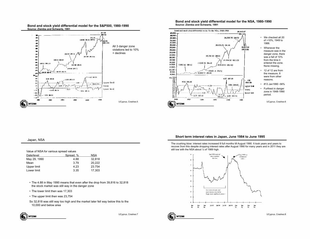
S&P500 index, PE ratios, government bond yields and the yield premium over stocks, January 1984 to August 1998.

Source: Ziemba and Schwartz, Invest Japan, 1991

Bond stock danger model (medium term)

enters danger zone

crash


•  Bonds and stocks compete for the money: strategic asset allocation.

•  Model was in the danger zone as early as April 1987 (S&P=289.32, then in August/September it moved further into the danger zone then there was a large fall in October 1987; S&P peak = 329.36 end August down to 245.01 at end of November 1987 (actual fall more)

•  Stocks continue to rally in danger zone but once they get in the zone, it is quite certain they will eventually fall, that is have a decline of 10% or more within one year.

Bond stock danger model cont�d


. !

All 3 danger zone violations led to 10%+ declines

Bond and stock yield differential model for the S&P500, 1980-1990 Source: Ziemba and Schwartz, 1991


. !

•  We checked all 20 of >10%, 1949 to 1988.

•  Whenever the measure was in the danger zone, there was a fall of 10% from the time it entered the zone. None missing.

•  12 of 12 are from the measure, 8 were from other reasons.

•  #13 Jan1990 -56%

•  Furthest in danger zone in 1948-1990 period.

Bond and stock yield differential model for the NSA, 1980-1990 Source: Ziemba and Schwartz, 1991


•  The 4.88 in May 1990 means that even after the drop from 39,816 to 32,818 the stock market was still way in the danger zone

•  The lower limit then was 17,303

•  The upper limit then was 23,754

So 32,818 was still way too high and the market later fell way below this to the 10,000 and below area

Value of NSA for various spread values Date/level Spread, % NSA May 29, 1990 4.88 32,818 Mean 3.79 20,222 Upper limit 4.23 23.754 Lower limit 3.35 17,303

Japan, NSA


. !

The crushing blow: interest rates increased 8 full months till August 1990. It took years and years to recover from this despite dropping interest rates after August 1990 for many years and in 2011 they are still low with the NSA about ¼ of 1989 high.

Short term interest rates in Japan, June 1984 to June 1995


. !

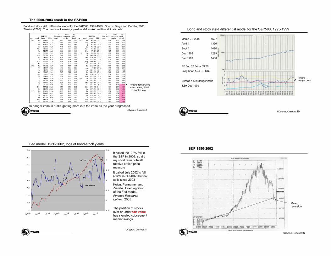
Bond and stock yield differential model for the S&P500, 1995-1999. Source: Berge and Ziemba, 2001, Ziemba (2003). The bond stock earnings yield model worked well to call that crash.

In danger zone in 1999, getting more into the zone as the year progressed.

The 2000-2003 crash in the S&P500

enters danger zone crash in Aug 2000, 16 months later


March 24, 2000 1527.46

April 4 1356.56

Sept 1 1420

Dec 1998 1229.23

Dec 1999 1460.25

PE flat, 32.34 → 33.29

Long bond 5.47 → 6.69

Spread >3, in danger zone

3.69 Dec 1999

Bond and stock yield differential model for the S&P500, 1995-1999

enters danger zone


WTZIMI

It called the -22% fall in the S&P in 2002; so did my short term put-call relative option price measure It called July 2002�s fall (-12% in 3Q2002) but no calls since 2003 Koivu, Pennamen and Ziemba, Co-integration of the Fed model, Finance Research Letters; 2005

The position of stocks over or under fair value has signaled subsequent market swings.

Fed model, 1980-2002, logs of bond-stock yields


S&P 1990-2002

Mean reversion


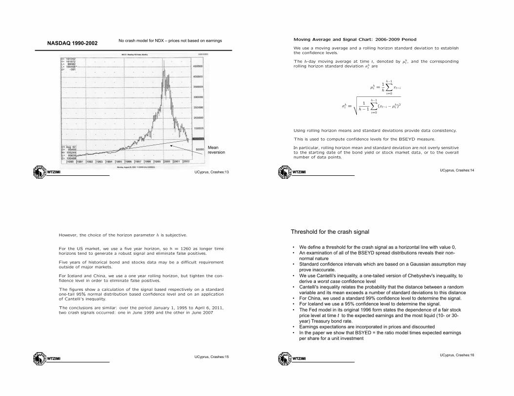
NASDAQ 1990-2002

Mean reversion

No crash model for NDX – prices not based on earnings


Moving Average and Signal Chart: 2006-2009 Period

We use a moving average and a rolling horizon standard deviation to establishthe confidence levels.

The h-day moving average at time t, denoted by µ

h

t

, and the correspondingrolling horizon standard deviation �

h

t

are

µ

h

t

=1

h

h�1X

i=0

x

t�i

�

h

t

=

vuut 1

h� 1

h�1X

i=0

(xt�i

� µ

h

t

)2

Using rolling horizon means and standard deviations provide data consistency.

This is used to compute confidence levels for the BSEYD measure.

In particular, rolling horizon mean and standard deviation are not overly sensitiveto the starting date of the bond yield or stock market data, or to the overallnumber of data points.


However, the choice of the horizon parameter h is subjective.

For the US market, we use a five year horizon, so h = 1260 as longer timehorizons tend to generate a robust signal and eliminate false positives.

Five years of historical bond and stocks data may be a di�cult requirementoutside of major markets.

For Iceland and China, we use a one year rolling horizon, but tighten the con-fidence level in order to eliminate false positives.

The figures show a calculation of the signal based respectively on a standardone-tail 95% normal distribution based confidence level and on an applicationof Cantelli’s inequality.

The conclusions are similar: over the period January 1, 1995 to April 6, 2011,two crash signals occurred: one in June 1999 and the other in June 2007

Threshold for the crash signal


•  We define a threshold for the crash signal as a horizontal line with value 0, •  An examination of all of the BSEYD spread distributions reveals their non-

normal nature •  Standard confidence intervals which are based on a Gaussian assumption may

prove inaccurate. •  We use Cantelli's inequality, a one-tailed version of Chebyshev's inequality, to

derive a worst case confidence level •  Cantelli's inequality relates the probability that the distance between a random

variable and its mean exceeds a number of standard deviations to this distance •  For China, we used a standard 99% confidence level to determine the signal. •  For Iceland we use a 95% confidence level to determine the signal. •  The Fed model in its original 1996 form states the dependence of a fair stock

price level at time t to the expected earnings and the most liquid (10- or 30-year) Treasury bond rate.

•  Earnings expectations are incorporated in prices and discounted •  In the paper we show that BSYED = the ratio model times expected earnings

per share for a unit investment

WTZIMI UCyprus, Crashes:

17

BSEYD Model

The idea behind the BSEYD model is that a crash signal should occur whenever

BSEY D(t) > CL(t)

where CL(t) represents a one-tail confidence level. The level CL acts as atime-varying threshold for the crash signal.

Equivalently, we define the signal directly as

SIGNAL(t) = BSEY D(t)� CL(t),

So, a crash signal should occur whenever

SIGNAL(t) = BSEY D(t)� CL(t) > 0.

Graphically, the threshold for the crash signal is now an horizontal line withvalue 0

Another motivation


•  A more theoretically sound motivation for the predictive ability of the BSEYD is using the basic Gordon formula, where EP is the forward earnings yield (which Schwartz and Ziemba (2000) show is the best predictor of at least individual Japanese stock prices),

E/P - nominal yield = equity risk premium - real growth - inflation.

•  So the BSEYD can be used as a proxy for the unobservable right hand side

economic variables. •  Koivu, Pennanen and Ziemba (2005) study the Fed model using a dynamic

vector equilibrium correction model with data from 1980 to 2003 in the US, UK and Germany and show that the Fed model had predictive power in forecasting equity prices, earnings and bond yields.

The model has been successful in predicting market turns


In spite of its empirical success and simplicity, the model has been justifiably criticized. •  First it does not consider the role played by time varying risk premiums in the

portfolio selection process while it does consider a risk free government interest rate as the discount factor of future earnings.

•  More seriously, the inflation illusion (the possible impact of inflation expectations on the stock market) as suggested by Modigliani and Cohn (1979) is not taken into consideration.

•  Thirdly, the model assumes the comparability of earning price ratios, a real quantity, with a nominal, bond induced, interest rate [Campbell and Vuolteenaho (2004), Asness (2000, 2003), and Ritter and Warr (2002) discuss these issues.] Consigli, MacLean, Zhao and Ziemba (2009) propose a stochastic model of equity returns based on an extension of the model inclusive of a risk premium in which market corrections are endogenously generated by the bond-stock yield difference.

•  The model accommodates both cases of prolonged yield deviations leading to a long series of small declines in the equity market and the case, peculiar of recent speculative bubbles, of a series of corrections over limited time periods.

•  The inclusion of the yield differential as a key driver of the market correction process is tested and the model is validated with market data

Comments


Many of the critics focus on: •  short term predictability that we know is weak as does Giot and Petitjean (2008), •  simply do not focus on the long run value of the measure, or •  dismiss it outright because of the nominal versus real minor flaw as does Montier

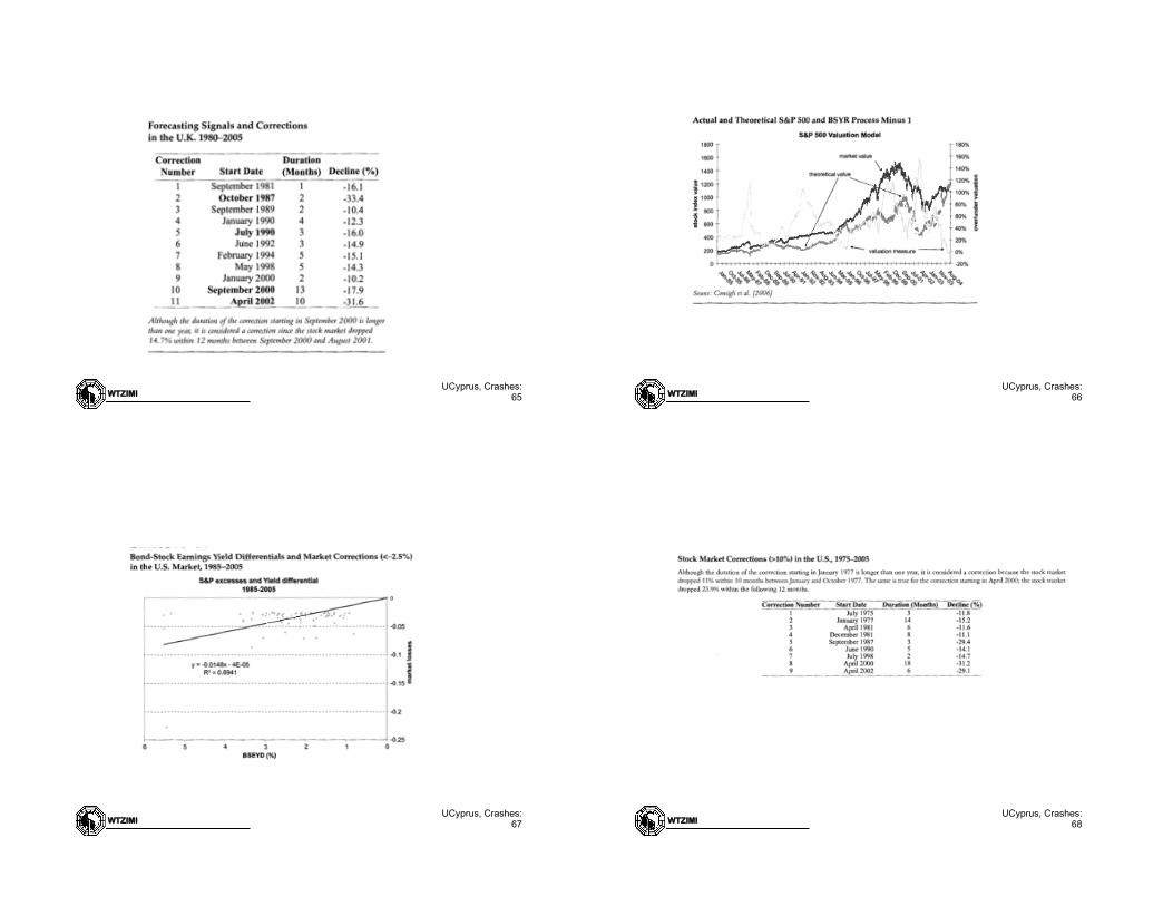
(2011). Consigli, MacLean, Zhao and Ziemba (2009) use the model to estimate the current fair value of the S&P500. •  Of course, market and fair value can diverge for long periods. •  Our concern is whether or not the model actually predicts stock market crashes,

stock market rallies and good times to be in and out of stock markets. •  Berge, Consigli and Ziemba (2008) discuss the latter issue and found for five

countries (US, Germany, Canada, UK and Japan) that the strategy stay in the market when it is not in the danger zone and move to cash otherwise provides about double the final wealth with less variance and a higher Sharpe ratio than a buy and hold strategy during 1975-2005 and 1980-2005 (see slides at end of talk)

•  There is some limited predictability of stock market increases but the evidence supports the good use of the model to predict crashes.



22

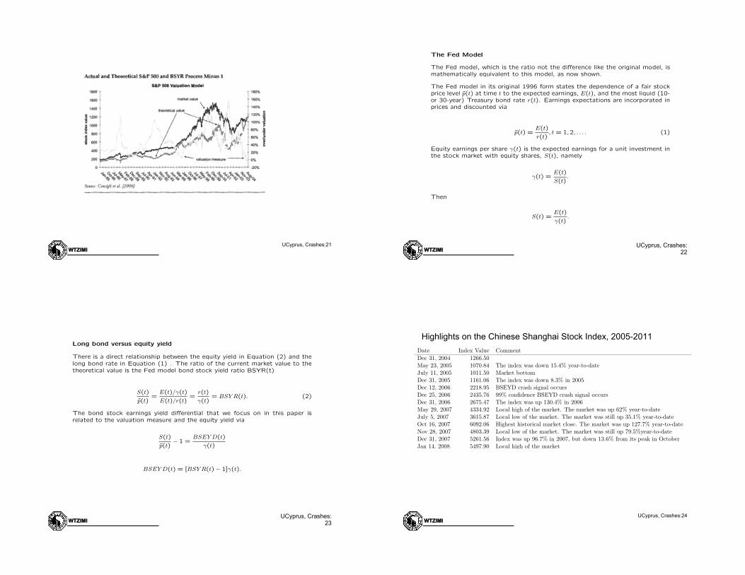
The Fed Model

The Fed model, which is the ratio not the di↵erence like the original model, is

mathematically equivalent to this model, as now shown.

The Fed model in its original 1996 form states the dependence of a fair stock

price level p̃(t) at time t to the expected earnings, E(t), and the most liquid (10-

or 30-year) Treasury bond rate r(t). Earnings expectations are incorporated in

prices and discounted via

p̃(t) =

E(t)

r(t), t = 1,2, . . . . (1)

Equity earnings per share �(t) is the expected earnings for a unit investment in

the stock market with equity shares, S(t), namely

�(t) =

E(t)

S(t).

Then

S(t) =

E(t)

�(t).

1


23

Long bond versus equity yield

There is a direct relationship between the equity yield in Equation (2) and the

long bond rate in Equation (1) . The ratio of the current market value to the

theoretical value is the Fed model bond stock yield ratio BSYR(t)

S(t)

p̃(t)=

E(t)/�(t)

E(t)/r(t)=

r(t)

�(t)= BSY R(t). (2)

The bond stock earnings yield di↵erential that we focus on in this paper is

related to the valuation measure and the equity yield via

S(t)

p̃(t)� 1 =

BSEY D(t)

�(t)

BSEY D(t) = [BSY R(t)� 1]�(t).

2

Highlights on the Chinese Shanghai Stock Index, 2005-2011


Stock market crashes Lleo and Ziemba

Table 2: Highlights on the Shanghai Stock Index, 2005-2011

Date Index Value CommentDec 31, 2004 1266.50May 23, 2005 1070.84 The index was down 15.4% year-to-dateJuly 11, 2005 1011.50 Market bottomDec 31, 2005 1161.06 The index was down 8.3% in 2005Dec 12, 2006 2218.95 BSEYD crash signal occursDec 25, 2006 2435.76 99% confidence BSEYD crash signal occursDec 31, 2006 2675.47 The index was up 130.4% in 2006May 29, 2007 4334.92 Local high of the market. The market was up 62% year-to-dateJuly 5, 2007 3615.87 Local low of the market. The market was still up 35.1% year-to-dateOct 16, 2007 6092.06 Highest historical market close. The market was up 127.7% year-to-dateNov 28, 2007 4803.39 Local low of the market. The market was still up 79.5%year-to-dateDec 31, 2007 5261.56 Index was up 96.7% in 2007, but down 13.6% from its peak in OctoberJan 14, 2008 5497.90 Local high of the marketJan 18, 2008 5180.51 The index closes the week at 5180.51,

which is 5.8% lower than than its local high on Jan 14Jan 21, 2008 4914.43 The index experiences a one-day drop of 5.1% from 5180.51 to 4914.43Jan 22, 2008 4559.75 The index experiences declines by 7.2% on this day,

opening at 4914.43 to close at 4559.75Jan 25, 2008 4761.69 The index recovers slightly to close the week at 4761.69Jan 28, 2008 4419.29 The index drops by 7.2% from 4761.69 to 4419.29Apr 18, 2008 3094.67 Local low of the marketMay 5, 2008 3761.01 Local high of the marketNov 4, 2008 1706.70 Global market minimum. The market was down by 72% peak to trough

and 23.09% and 29.93% from the December 12 and 25 danger signal levelsDec 31, 2008 1820.81 The market was down 65.4% in 2008Aug 3, 2009 3471.44 Local high of the market. The market was up 103.4% from the troughAug 31, 2009 2667.75 Local low of the marketNov 23, 2009 3338.66 Local high of the marketDec 31, 2009 3277.14 The market was up 80% in 2009Jul 5, 20100 2363.95 Local low of the marketDec 31, 2010 2808.08 The market was down 14.3% in 2009Apr 30, 2011 2911.51 The market was up 3.7% year-to-date

10

Shanghai highlights cont’d


October 30, 2011 23:5 Quantitative Finance crashes˙QF

Quantitative Finance, Vol. 00, No. 00, Month 200x, 8–35

Table 2. Highlights on the Shanghai Stock Index, 2005-2011Date Index Value CommentDec 31, 2004 1266.50May 23, 2005 1070.84 The index was down 15.4% year-to-dateJuly 11, 2005 1011.50 Market bottomDec 31, 2005 1161.06 The index was down 8.3% in 2005Dec 12, 2006 2218.95 95% confidence BSEYD crash signal occursDec 25, 2006 2435.76 99% confidence BSEYD crash signal occursDec 31, 2006 2675.47 The index was up 130.4% in 2006May 29, 2007 4334.92 Local high of the market. The market was up 62% year-to-dateJuly 5, 2007 3615.87 Local low of the market. The market was still up 35.1% year-to-dateOct 16, 2007 6092.06 Highest historical market close. The market was up 127.7% year-to-dateNov 28, 2007 4803.39 Local low of the market. The market was still up 79.5%year-to-dateDec 31, 2007 5261.56 Index was up 96.7% in 2007, but down 13.6% from its peak in OctoberJan 14, 2008 5497.90 Local high of the marketJan 18, 2008 5180.51 The index closes the week at 5180.51,

which is 5.8% lower than than its local high on Jan 14Jan 21, 2008 4914.43 The index experiences a one-day drop of 5.1% from 5180.51 to 4914.43Jan 22, 2008 4559.75 The index experiences declines by 7.2% on this day,

opening at 4914.43 to close at 4559.75Jan 25, 2008 4761.69 The index recovers slightly to close the week at 4761.69Jan 28, 2008 4419.29 The index drops by 7.2% from 4761.69 to 4419.29Apr 18, 2008 3094.67 Local low of the marketMay 5, 2008 3761.01 Local high of the marketNov 4, 2008 1706.70 Global market minimum. The market was down by 72% peak to trough

and 23.09% and 29.93% from the December 12 and 25 danger signal levelsDec 31, 2008 1820.81 The market was down 65.4% in 2008Aug 3, 2009 3471.44 Local high of the market. The market was up 103.4% from the troughAug 31, 2009 2667.75 Local low of the marketNov 23, 2009 3338.66 Local high of the marketDec 31, 2009 3277.14 The market was up 80% in 2009Jul 5, 20100 2363.95 Local low of the marketDec 31, 2010 2808.08 The market was down 14.3% in 2009Jun 30, 2011 2762.08 The market was down about 1% year-to-dateAugust 31, 2011 2567.34 The market was down about 8.6% year-to-dateSeptember 30, 2011 2359.22 The market was down about 16% year-to-date

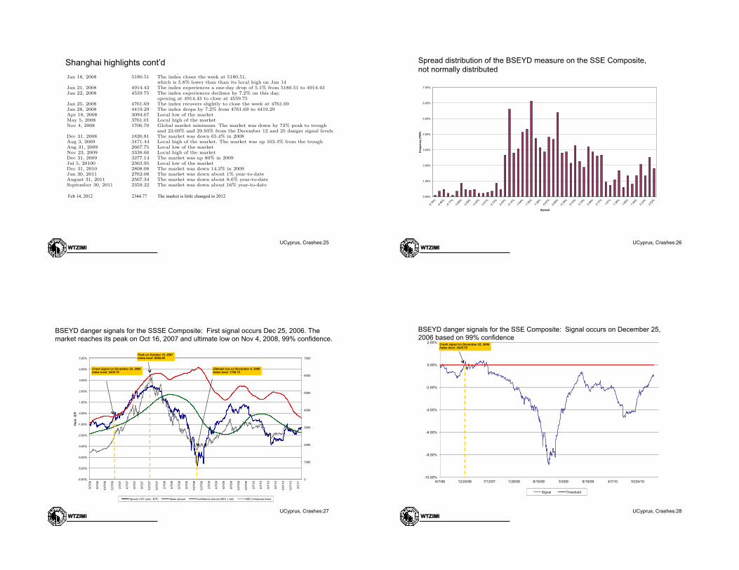
Figure 4 also illustrates the importance of the confidence level in relation to the rolling hori-zon of the moving average and the shape of the spread distribution. As pointed out in Section2, a short time horizon of one year, combined with a lower confidence level of 95% and thenon-Gaussian nature of the spread distribution may result in false positives. An ex-post anal-ysis reveals that the Gaussian-based 95% confidence spread for the Shanghai Stock ExchangeComposite index over the entire period equals 1.78%. However, the actual 95% confidence levelof the empirical distribution is 2.18%. In fact, a full 9.32% of all actual observations occur at orabove 1.78%, a marked contrast from the 5% predicted by the Gaussian distribution. Raisingthe confidence level to 99% or increasing the rolling horizon does help reduce the impact of theshape of the distribution on the signal.

Feb 14, 2012 2344.77 The market is little changed in 2012

Spread distribution of the BSEYD measure on the SSE Composite, not normally distributed


0.00%

1.00%

2.00%

3.00%

4.00%

5.00%

6.00%

7.00%

Freq

uenc

y (P

DF)

Spread

Spread distribution: !anything but Normally distributed!

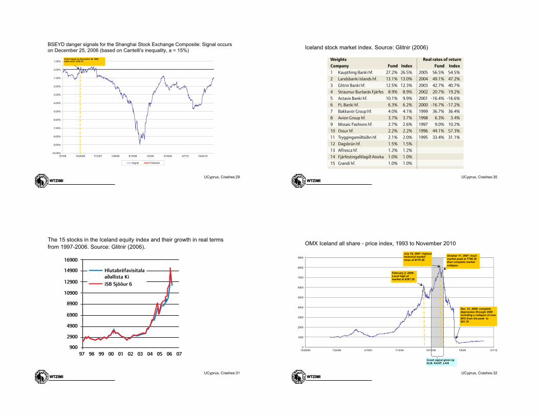
BSEYD danger signals for the SSSE Composite: First signal occurs Dec 25, 2006. The market reaches its peak on Oct 16, 2007 and ultimate low on Nov 4, 2008, 99% confidence.


0

1000

2000

3000

4000

5000

6000

7000

-6.00%

-5.00%

-4.00%

-3.00%

-2.00%

-1.00%

0.00%

1.00%

2.00%

3.00%

4.00%

5.00%

6/7/

06

8/7/

06

10/7

/06

12/7

/06

2/7/

07

4/7/

07

6/7/

07

8/7/

07

10/7

/07

12/7

/07

2/7/

08

4/7/

08

6/7/

08

8/7/

08

10/7

/08

12/7

/08

2/7/

09

4/7/

09

6/7/

09

8/7/

09

10/7

/09

12/7

/09

2/7/

10

4/7/

10

6/7/

10

8/7/

10

10/7

/10

12/7

/10

2/7/

11

Yiel

d - E

/P

Spread (10Y yield - E/P) Mean spread Confidence interval (99% 1-tail) SSE Composite Index

Crash signal on December 25, 2006 Index level: 2435.76

Peak on October 16, 2007 Index level: 6092.06

Ultimate low on November 4, 2008 Index level: 1706.70

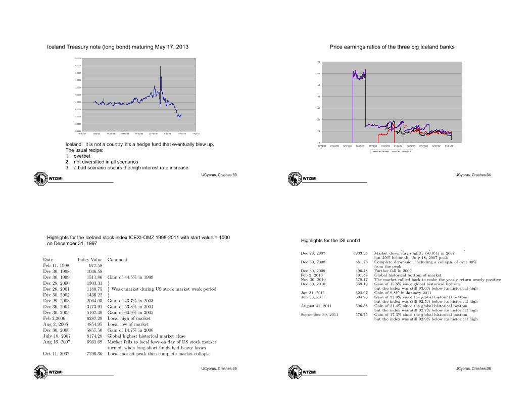
BSEYD danger signals for the SSE Composite: Signal occurs on December 25, 2006 based on 99% confidence


-10.00%

-8.00%

-6.00%

-4.00%

-2.00%

0.00%

2.00%

6/7/06 12/24/06 7/12/07 1/28/08 8/15/08 3/3/09 9/19/09 4/7/10 10/24/10

Signal Threshold


BSEYD danger signals for the Shanghai Stock Exchange Composite: Signal occurs on December 25, 2006 (based on Cantelli's inequality, a = 15%)


-10.00%

-9.00%

-8.00%

-7.00%

-6.00%

-5.00%

-4.00%

-3.00%

-2.00%

-1.00%

0.00%

1.00%

6/7/06 12/24/06 7/12/07 1/28/08 8/15/08 3/3/09 9/19/09 4/7/10 10/24/10

Signal Threshold


Iceland stock market index. Source: Glitnir (2006)


30 WILMOTT magazine

high interest rates may begin to have a negativeimpact on growth and financial assets (see Figure9). The CBI is well managed and will likely droprates in 2007 but it is easy to overshoot here. WTZpoints to the example of Japan where the BOJ

raised rates in 1988-89. They continued to do soeven after the stock market began to fall inJanuary 1990 and proceeded to raise rates tillAugust 1990, a full 8 months more. This was amajor cause of many bankruptcies and the 15-

year slump in Japan’s economic andfinancial markets. However in anenvironment of global tightening,especially with the Fed unlikely tostop tightening until September2006 at the earliest, the CBI may beunable to get out of step for fear of adecreasing interest rate differential,even if that results in an overshoot.Given high and rising inflation inIceland, the CBI will have domesticreasons to continue to raise interestrates.

Many have spoken about a possi-ble housing bubble. A governmentpolicy of subsidizing interest rates at5 per cent for personal housing is onecontributing factor encouraging thisoverheating. However, commercialand industry held property does notbenefit from this subsidy. However,the policy of many companies of sell-ing property and leasing it back toaccess further credit many have con-tributed to this boom. It is hard notto foresee trouble in the housing sec-tor especially with steady increases innominal prices since 2002 and yearlygains in the 30-40 per cent range in2004 and 2005 and a 20 per cent rise

the first half of 2006. Since there is an increasedsupply of land, much construction, a softeningmarket with prices higher than constructioncosts, coupled with the higher interest rates, lesscredit available for housing loans, declining con-sumer confidence, the prediction of Glitnir(2006) that nominal prices might decline 5-10 percent in 2007 might even be optimistic. A keyquestion is whether they will fall softly or therewill be a hard landing.

Financial (in)stability?In their report, which responds to many of thevulnerability analyses of Iceland, Mishkin andHerbertsson (2006) drawing from the economicliterature, argue that there none of three routesto financial instability are present in theIcelandic situation of today. These drivers ofinstability are:

1. financial liberalization with weak pruden-tial regulation and supervision;

2. severe fiscal imbalances; and 3. imprudent monetary policy.They conclude that the economy has adjusted

to financial liberalization and there is prudentregulation and effective supervision. There gov-ernment debt has decreased to low levels and thepension system is fully funded. Monetary policyhas kept core inflation (excluding housing) on

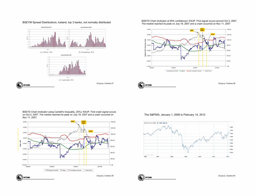
Table 7: Stock market index. Source: Glitnir (2006b)Weights Real rates of returnCompany Fund Index Fund Index1 Kaupthing Banki hf. 27.2% 26.5% 2005 56.5% 54.5%2 Landsbanki Islands hf. 13.1% 13.0% 2004 49.1% 47.2%3 Glitnir Banki hf. 12.5% 12.3% 2003 42.7% 40.7%4 Straumur Buróarás Fjárfes 8.9% 8.9% 2002 20.7% 19.2%5 Actavis Banki hf. 10.1% 9.9% 2001 -16.4% -16.6%6 FL Banki hf. 6.3% 6.2% 2000 -16.7% -17.2%7 Bakkavör Group hf. 4.0% 4.1% 1999 36.7% 36.4%8 Avion Group hf. 3.7% 3.7% 1998 6.3% 3.4%9 Mosaic Fashions hf. 2.7% 2.6% 1997 9.0% 10.2%10 Ossur hf. 2.2% 2.2% 1996 44.1% 57.3%11 Tryggingami!tö!in hf. 2.1% 2.0% 1995 33.4% 31.1%12 Dagsbrún hf. 1.5% 1.5%13 Alfresca hf. 1.2% 1.2%14 Fjárfestingafélagi! Atorka 1.0% 1.0%15 Grandi hf. 1.0% 1.0%

16900

14900

12900

10900

8900

6900

4900

2900

90097 98 99 00 01 02 03 04 05 06 07

iSB Sjóôur 6

Hlutabréfavisitala a!allista Ki

Figure 10: The 15 stocks in the Iceland equityindex and their growth in real terms from 1997-2006. Source: Glitnir (2006b)

16%15%14%13%12%11%10%9%8%7%6%5%4%Jan. 03 Jul. 03 Jan. 04 Jul. 04 Jan. 05 Jul. 05 Jan. 06 Jul. 06 Jan. 07 Jul. 07

Figure 9: short interest rates 2003-2007. Source: Glitnir (2006a)

Table 6: Long-bond (10 yr) versus earning yield differentials for major countries, July 12, 2006

S&P500 FTSE200 Nikkei225 CAC40 DAX30index 1259 5861 15249 4942 5638

A) PE ratio 16.86 16.61 36.26 13.82 13.33B) Stock Return (1/A) 5.93% 6.02% 2.76% 7.24% 7.50%C) Bond Return (10 yr) 5.10% 4.67% 1.94% 4.10% 4.09%Crash Signal (C-B) -0.83 -1.35 -0.82 -3.14 -3.41

BILL ZIEMBA

The 15 stocks in the Iceland equity index and their growth in real terms from 1997-2006. Source: Glitnir (2006).


16900

14900

12900

10900

8900

6900

4900

2900

90097 98 99 00 01 02 03 04 05 06 07

iSB Sjóôur 6

Hlutabréfavisitala a!allista Ki

OMX Iceland all share - price index, 1993 to November 2010


0

1000

2000

3000

4000

5000

6000

7000

8000

9000

10/28/95 7/24/98 4/19/01 1/14/04 10/10/06 7/6/09 4/1/12

October 11, 2007: local market peak at 7796.36 then complete market collapse

July 18, 2007: highest historical market close at 8174.28

Dec. 31, 2008: complete depression through 2008 including a collapse of over 90% from the peak to 581.76

February 2, 2006: Local high of market at 6287.29

Crash signal given by GLB, KAUP, LAIS

Iceland Treasury note (long bond) maturing May 17, 2013


Treasury note maturing May 17th 2013

0.0000

2.0000

4.0000

6.0000

8.0000

10.0000

12.0000

14.0000

16.0000

18.0000

20.0000

19-Apr-01 1-Sep-02 14-Jan-04 28-May-05 10-Oct-06 22-Feb-08 6-Jul-09 18-Nov-10 1-Apr-12

Iceland: it is not a country, it’s a hedge fund that eventually blew up. The usual recipe: 1.  overbet 2.  not diversified in all scenarios 3.  a bad scenario occurs the high interest rate increase

Price earnings ratios of the three big Iceland banks


0

10

20

30

40

50

60

70

07/24/98 07/24/99 07/23/00 07/23/01 07/23/02 07/23/03 07/22/04 07/22/05 07/22/06 07/22/07 07/21/08

P/E Icelandic Banks

Landbsbanki Kau GLB

Highlights for the Iceland stock index ICEXI-OMZ 1998-2011 with start value = 1000 on December 31, 1997



Table 4: Highlights for the Iceland stock index ICEXI-OMZ 1998-2011 with start value =1000 on December 31, 1997

Date Index Value CommentFeb 11, 1998 977.58Dec 30, 1998 1046.58Dec 30, 1999 1511.86 Gain of 44.5% in 1999Dec 28, 2000 1303.31 }Dec 28, 2001 1180.75 } Weak market during US stock market weak periodDec 30, 2002 1436.22 }Dec 29, 2003 2064.05 Gain of 43.7% in 2003Dec 30, 2004 3173.91 Gain of 53.8% in 2004Dec 30, 2005 5107.49 Gain of 60.9% in 2005Feb 2,2006 6287.29 Local high of marketAug 2, 2006 4854.95 Local low of marketDec 30, 2006 5857.50 Gain of 14.7% in 2006July 18, 2007 8174.28 Global highest historical market closeAug 16, 2007 6931.69 Market falls to local lows on day of US stock market

turmoil when long-short funds had heavy lossesOct 11, 2007 7796.36 Local market peak then complete market collapseDec 28, 2007 5803.35 Market down just slightly (-0.9%) in 2007

but -% below the July 28, 2007 peakDec 30, 2008 581.76 Complete depression including a collapse of over 90%

from the peak and during 2008Dec 30, 2008 496.48 Further fall in 2009Feb 2, 2010 491.58 Global historical bottom of marketNov 30, 2010 579.17 The market rallied back to make the yearly return nearly positiveDec 30, 2010 569.19 Gain of 15.8% since global historical bottom

but the index still 93.0% below its historical highJan 31, 2011 624.97 Gain of 9.8% in January 2011April 30, 2011 626.76 Gain of 27.5% since the global historical bottom

but the index is still 92.3% below its historical high

20

Highlights for the ISI cont’d




Figure 10. Iceland Treasury note (long bond) maturing May 17, 2013

Table 4. Highlights for the Iceland stock index ICEXI-OMZ 1998-2011 with start value = 1000 onDecember 31, 1997

Date Index Value CommentFeb 11, 1998 977.58Dec 30, 1998 1046.58Dec 30, 1999 1511.86 Gain of 44.5% in 1999Dec 28, 2000 1303.31 }Dec 28, 2001 1180.75 } Weak market during US stock market weak periodDec 30, 2002 1436.22 }Dec 29, 2003 2064.05 Gain of 43.7% in 2003Dec 30, 2004 3173.91 Gain of 53.8% in 2004Dec 30, 2005 5107.49 Gain of 60.9% in 2005Feb 2,2006 6287.29 Local high of marketAug 2, 2006 4854.95 Local low of marketDec 30, 2006 5857.50 Gain of 14.7% in 2006July 18, 2007 8174.28 Global highest historical market closeAug 16, 2007 6931.69 Market falls to local lows on day of US stock market

turmoil when long-short funds had heavy lossesOct 11, 2007 7796.36 Local market peak then complete market collapseDec 28, 2007 5803.35 Market down just slightly (-0.9%) in 2007

but 29% below the July 18, 2007 peakDec 30, 2008 581.76 Complete depression including a collapse of over 90%

from the peakDec 30, 2009 496.48 Further fall in 2009Feb 2, 2010 491.58 Global historical bottom of marketNov 30, 2010 579.17 The market rallied back to make the yearly return nearly positiveDec 30, 2010 569.19 Gain of 15.8% since global historical bottom

but the index was still 93.0% below its historical highJan 31, 2011 624.97 Gain of 9.8% in January 2011Jun 30, 2011 604.95 Gain of 23.0% since the global historical bottom

but the index was still 92.5% below its historical highAugust 31, 2011 596.58 Gain of 21.4% since the global historical bottom

but the index was still 92.7% below its historical highSeptember 30, 2011 576.75 Gain of 17.3% since the global historical bottom

but the index was still 92.9% below its historical high

on September 28, 2007, two months after the July 18 peak and less than a month before theNovember 11 crash. For Glitnir, the signal was much earlier on October 17, 2006, some thirteenmonths before the crash. Finally, for Lansbanki, the danger signal was on February 13, 2007.Figures 12bdf show the BSEYM using Cantelli’s inequality to account for the non-normality of

Quantitative Finance

ISSN 1469-7688 print/ISSN 1469-7696 online c� 200x Taylor & Francis

http://www.tandf.co.uk/journalsDOI: 10.1080/1469768YYxxxxxxxx

BSEYM Spread Distributions, Iceland, top 3 banks, not normally distributed



0.00%

1.00%

2.00%

3.00%

4.00%

5.00%

6.00%

7.00%

Freq

uenc

y

Spread

Spread Distribution GLB

(a) Glitnir, MA

0.00%

1.00%

2.00%

3.00%

4.00%

5.00%

6.00%

7.00%

Freq

uenc

y

Spread

Spread Distribution KAUP

(b) Kaupthing, MA

0.00%

1.00%

2.00%

3.00%

4.00%

5.00%

6.00%

7.00%

Freq

uenc

y

Spread

Spread Distribution LAIS

(c) Lansbanki, MA

Figure 11: BSEYM Spread Distributions, Iceland

21

BSEYD Chart (Indicator at 95% confidence): KAUP. First signal occurs around Oct 2, 2007. The market reached its peak on July 18, 2007 and a crash occurred on Nov 11, 2007


0.00

200.00

400.00

600.00

800.00

1000.00

1200.00

1400.00

-0.1000

-0.0800

-0.0600

-0.0400

-0.0200

0.0000

0.0200

0.0400

5/28/05 5/28/06 5/28/07 5/27/08

ln(B

ond

Yie

ld /

Ear

ning

s Y

ield

)

Spread for KAUP Mean 95% Confidence Interval Stock Price

crash signal peak

crash

BSEYD Chart (Indicator using Cantelli's Inequality, 20%): KAUP. First crash signal occurs on Oct 2, 2007. The market reached its peak on July 18, 2007 and a crash occurred on Nov 11, 2007.


0.00

200.00

400.00

600.00

800.00

1000.00

1200.00

1400.00

-10.00%

-8.00%

-6.00%

-4.00%

-2.00%

0.00%

2.00%

4.00%

6.00%

5/28/05 5/28/06 5/28/07 5/27/08

Yiel

d - E

/P

Spread for KAUP Mean Confidence Interval Stock Price

crash signal

peak

crash

The S&P500, January 1, 2006 to February 14, 2012


Highlights of the S&P500, January 1, 2006 to April 30, 2011



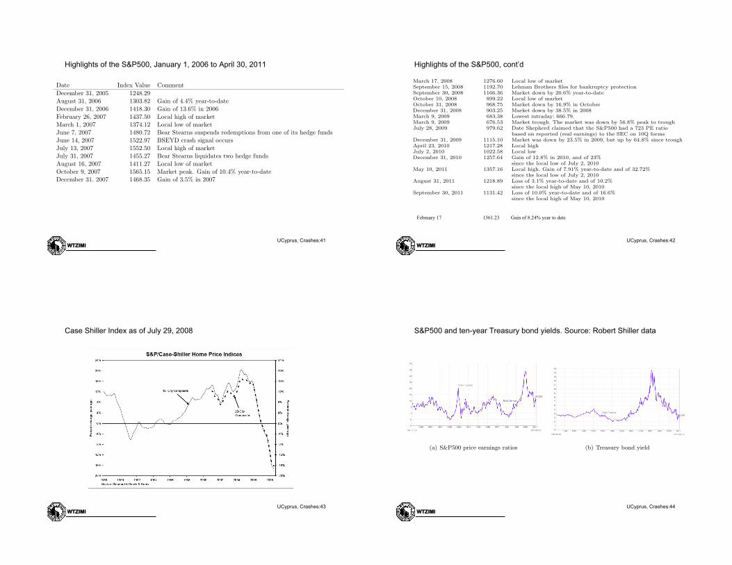
Table 7: Highlights of the S&P500, January 1, 2006 to April 30, 2011

Date Index Value CommentDecember 31, 2005 1248.29August 31, 2006 1303.82 Gain of 4.4% year-to-dateDecember 31, 2006 1418.30 Gain of 13.6% in 2006February 26, 2007 1437.50 Local high of marketMarch 1, 2007 1374.12 Local low of marketJune 7, 2007 1480.72 Bear Stearns suspends redemptions from one of its hedge fundsJune 14, 2007 1522.97 BSEYD crash signal occursJuly 13, 2007 1552.50 Local high of marketJuly 31, 2007 1455.27 Bear Stearns liquidates two hedge fundsAugust 16, 2007 1411.27 Local low of marketOctober 9, 2007 1565.15 Market peak. Gain of 10.4% year-to-dateDecember 31, 2007 1468.35 Gain of 3.5% in 2007March 17, 2008 1276.60 Local low of marketSeptember 15, 2008 1192.70 Lehman Brothers files for bankruptcy protectionSeptember 30, 2008 1166.36 Market down by 20.6% year-to-dateOctober 10, 2008 899.22 Local low of marketOctober 31, 2008 968.75 Market down by 16.9% in OctoberDecember 31, 2008 903.25 Market down by 38.5% in 2008March 9, 2009 683.38 Lowest intraday: 666.79.March 9, 2009 676.53 Market trough. The market was down by 56.8% peak to troughJuly 28, 2009 979.62 Date Shepherd claimed that the S&P500 had a 723 PE ratio

based on reported (real earnings) to the SEC on 10Q formsDecember 31, 2009 1115.10 Market was down by 23.5% in 2009, but up by 64.8% since troughApril 23, 2010 1217.28 Local highJuly 2, 2010 1022.58 Local lowDecember 31, 2010 1257.64 Gain of 12.8% in 2010, and of 23%

since the local low of July 6, 2010April 31, 2011 1363.61 Gain of 8.4% year-to-date and of 33.3%

since the local low of July 6, 2010

31

Highlights of the S&P500, cont’d




Table 7. Highlights of the S&P500, January 1, 2006 to April 30, 2011Date Index Value CommentDecember 31, 2005 1248.29August 31, 2006 1303.82 Gain of 4.4% year-to-dateDecember 31, 2006 1418.30 Gain of 13.6% in 2006February 26, 2007 1437.50 Local high of marketMarch 1, 2007 1374.12 Local low of marketJune 7, 2007 1480.72 Bear Stearns suspends redemptions from one of its hedge fundsJune 14, 2007 1522.97 BSEYD crash signal occursJuly 13, 2007 1552.50 Local high of marketJuly 31, 2007 1455.27 Bear Stearns liquidates two hedge fundsAugust 16, 2007 1411.27 Local low of marketOctober 9, 2007 1565.15 Market peak. Gain of 10.4% year-to-dateDecember 31, 2007 1468.35 Gain of 3.5% in 2007March 17, 2008 1276.60 Local low of marketSeptember 15, 2008 1192.70 Lehman Brothers files for bankruptcy protectionSeptember 30, 2008 1166.36 Market down by 20.6% year-to-dateOctober 10, 2008 899.22 Local low of marketOctober 31, 2008 968.75 Market down by 16.9% in OctoberDecember 31, 2008 903.25 Market down by 38.5% in 2008March 9, 2009 683.38 Lowest intraday: 666.79.March 9, 2009 676.53 Market trough. The market was down by 56.8% peak to troughJuly 28, 2009 979.62 Date Shepherd claimed that the S&P500 had a 723 PE ratio

based on reported (real earnings) to the SEC on 10Q formsDecember 31, 2009 1115.10 Market was down by 23.5% in 2009, but up by 64.8% since troughApril 23, 2010 1217.28 Local highJuly 2, 2010 1022.58 Local lowDecember 31, 2010 1257.64 Gain of 12.8% in 2010, and of 23%

since the local low of July 2, 2010May 10, 2011 1357.16 Local high. Gain of 7.91% year-to-date and of 32.72%

since the local low of July 2, 2010August 31, 2011 1218.89 Loss of 3.1% year-to-date and of 10.2%

since the local high of May 10, 2010September 30, 2011 1131.42 Loss of 10.0% year-to-date and of 16.6%

since the local high of May 10, 2010

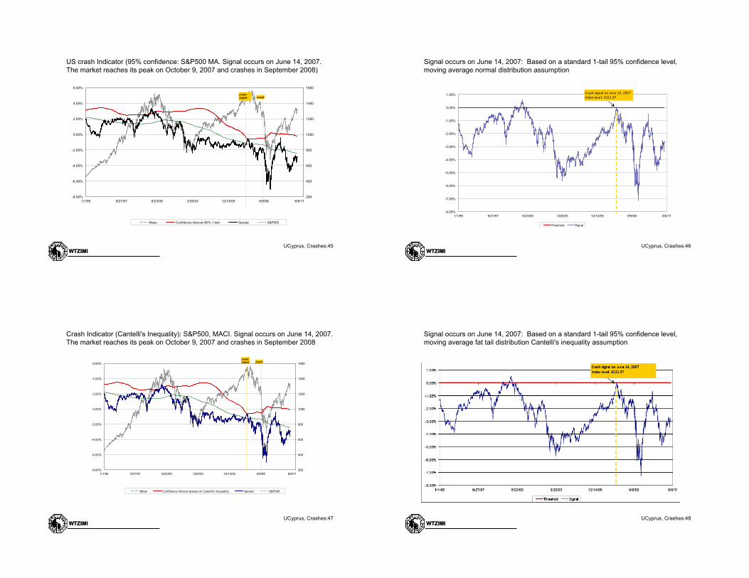
Table 7 lists some of the main events regarding the S&P500 from 2006 to 2011. There arenumerous books concerning this period plus many articles and columns. Ziemba has several inWilmott. Starting in June 2007, he designed strategies and traded for an o↵shore BVI basedhedge fund for a group headed by a top trader Nikolai Battoo. Battoo and his hedge funds hadinvestments in Bear Stearns and in June 2007 asked for his money back. That took three monthsand gave him a strong signal of danger. As an astute trader, he hedged and studied carefullythe market situation through technical indicators that he has developed. Ziemba remembershis words to him starting in the summer of 2007 “this is the big one” ...“eventually the marketwill go to 660 on the S&P500”. In the fall of 2007 the S&P500 was about 1500, see Figure 14.So this was a rather bold call but a private one and it turned out to be very accurate. NourielRoubini was predicting very boldly a serious financial meltdown starting in 2006 when thehousing market was beginning its decline; see Figure 15 which gives the Case Shiller Home PriceIndex as of July 24, 2008. There was a sharp decline from 2005 to 2008. He and other bearssuch as Yale Professor Robert Shiller are still (October 2011) pessimistic about the economy,real estate and financial markets. Dropping real estate has several depressive e↵ects such ashomeowners can no longer use house price gains to fund consumption, foreclosures, etc. TheMarch 2009 low closing was 676.53 with an intraday low of 660 on March 6. The subsequentrally has doubled the S&P500 to 1320.64 as of the end of June 2011. There is considerablediscussion regarding whether or not this rally is low interest rate related to the Fed quantitativeeasing, or only game in town since real estate, bonds and cash look unattractive. This is a casewhen the BSEYM signaled the rise in stock prices. A volatile period followed the rally, with adrop in the level of the S&P500 in August and September followed by a a stabilization in October.




February 17 1361.23 Gain of 8.24% year to date

Case Shiller Index as of July 29, 2008


S&P500 and ten-year Treasury bond yields. Source: Robert Shiller data



Figure 15: Case Shiller Index as of July 29, 2008.

WTZIMI 74

S&P500 PE Ratio

(a) S&P500 price earnings ratios

WTZIMI 75

10 year Treasury yield

(b) Treasury bond yield

Figure 16: S&P500 and ten-year Treasury bond yields. Source: Robert Shiller data.

32

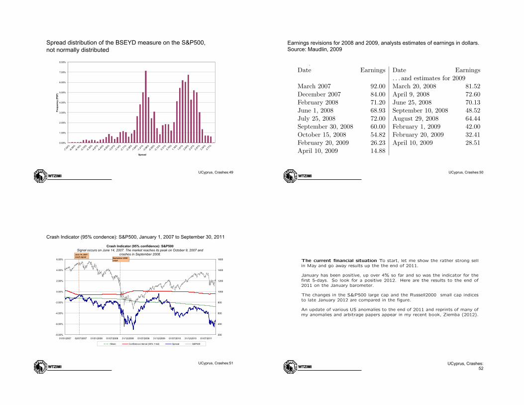
US crash Indicator (95% confidence: S&P500 MA. Signal occurs on June 14, 2007. The market reaches its peak on October 9, 2007 and crashes in September 2008)


200

400

600

800

1000

1200

1400

1600

-8.00%

-6.00%

-4.00%

-2.00%

0.00%

2.00%

4.00%

6.00%

1/1/95 9/27/97 6/23/00 3/20/03 12/14/05 9/9/08 6/6/11

Mean Confidence interval (95% 1-tail) Spread S&P500

crash signal crash

Signal occurs on June 14, 2007: Based on a standard 1-tail 95% confidence level, moving average normal distribution assumption


-8.00%

-7.00%

-6.00%

-5.00%

-4.00%

-3.00%

-2.00%

-1.00%

0.00%

1.00%

1/1/95 9/27/97 6/23/00 3/20/03 12/14/05 9/9/08 6/6/11

Signal occurs on June 14, 2007 (based on a standard 1-tail 95% confidence level)

Threshold Signal

Crash&signal&on&June&14,&2007&Index&level:&1522.97&

Crash Indicator (Cantelli's Inequality): S&P500, MACI. Signal occurs on June 14, 2007. The market reaches its peak on October 9, 2007 and crashes in September 2008


200

400

600

800

1000

1200

1400

1600

-8.00%

-6.00%

-4.00%

-2.00%

0.00%

2.00%

4.00%

6.00%

1/1/95 9/27/97 6/23/00 3/20/03 12/14/05 9/9/08 6/6/11

Mean Confidence interval (based on Canteli's inequality) Spread S&P500

crash signal crash

Signal occurs on June 14, 2007: Based on a standard 1-tail 95% confidence level, moving average fat tail distribution Cantelli's inequality assumption


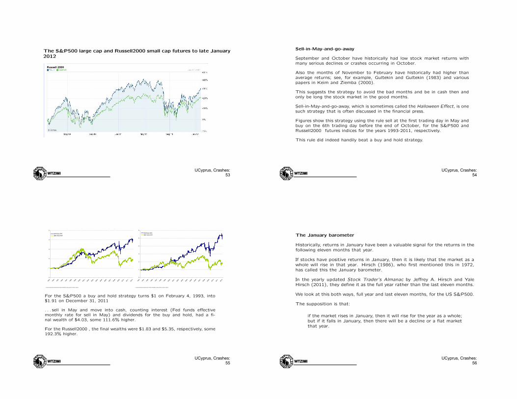
Spread distribution of the BSEYD measure on the S&P500, not normally distributed


0.00%

1.00%

2.00%

3.00%

4.00%

5.00%

6.00%

7.00%

8.00%

Freq

uenc

y (P

DF)

Spread

Spread distribution: anything but Normally distributed!

Earnings revisions for 2008 and 2009, analysts estimates of earnings in dollars. Source: Maudlin, 2009



Figure 19: Spread distribution of the BSEYD measure on the S&P500.

2007-2009 period. Table 8 has the S&P500 2008 estimated earnings and 2009 forecastedearnings. On July 25, 2008, the S&P500 earnings for 2008 were estimated to be 72.00 withthe S&P500 at 1257.76 which gives a PE ratio of 17.47 which is not high enough to signalthe September 2008 to March 2009 crash. But by February 20, 2009, the 2008 earningswere estimated to be only 26.23. With the S&P500 at 770.05 on that day the trailing PEratio was 29.36 which gives a BSEYD value of 2.78-(100/29.36) = -0.626.

Table 8: Earnings revisions for 2008 and 2009, analysts estimates of earnings in dollars.Source: Maudlin, 2009

Date Earnings Date Earnings. . . and estimates for 2009

March 2007 92.00 March 20, 2008 81.52December 2007 84.00 April 9, 2008 72.60February 2008 71.20 June 25, 2008 70.13June 1, 2008 68.93 September 10, 2008 48.52July 25, 2008 72.00 August 29, 2008 64.44September 30, 2008 60.00 February 1, 2009 42.00October 15, 2008 54.82 February 20, 2009 32.41February 20, 2009 26.23 April 10, 2009 28.51April 10, 2009 14.88

Shepherd (2009) has the S&P500 PE ratio at 723 on July 28, 2009 four months into therally that began in March 2009! The S&P500 was then 979.62. This high PE ratio was

34

Crash Indicator (95% condence): S&P500, January 1, 2007 to September 30, 2011




200

400

600

800

1000

1200

1400

1600

-8.00%

-6.00%

-4.00%

-2.00%

0.00%

2.00%

4.00%

6.00%

01/01/2007 02/07/2007 01/01/2008 01/07/2008 31/12/2008 01/07/2009 31/12/2009 01/07/2010 31/12/2010 01/07/2011

Crash Indicator (95% confidence): S&P500 Signal occurs on June 14, 2007. The market reaches its peak on October 9, 2007 and

crashes in September 2008.

Mean Confidence interval (95% 1-tail) Spread S&P500

June 14, 2007: crash signal September 2008:

crash

Figure 21. Crash Indicator (95% confidence): S&P500, January 1, 2007 to September 30, 2011

lnBSEY R(t) = ln

✓r(t)

�(t)

◆= ln r(t)� ln �(t).

For China and Iceland, both measures produce similar results which are available from theauthors. The pattern and timing of the crash signals nearly coincide for all three Icelandicbanks. In China, the lnBSEYR generates a slightly earlier signal than the BSEYD.

In the US, the result of the lnBSEYR and of the BSEYD measures are also broadly similar. Asignal precedes both the internet-related crash of 2000 and the credit crunch crash of 2008. Inaddition, the logarithmic lnBSYR(t) measure generates a signal in April 1998, ahead of a 19%decline from July 17th to August 31st. However, neither measure predicted the market declineof 2002. This is a combined result of the relatively low level reached by the two measures in2001 compared to 1999, and of the increase in the confidence level starting in 2000.





52

The current financial situation To start, let me show the rather strong sellin May and go away results up the the end of 2011.

January has been positive, up over 4% so far and so was the indicator for thefirst 5-days. So look for a positive 2012. Here are the results to the end of2011 on the January barometer.

The changes in the S&P500 large cap and the Russell2000 small cap indicesto late January 2012 are compared in the figure.

An update of various US anomalies to the end of 2011 and reprints of many ofmy anomalies and arbitrage papers appear in my recent book, Ziemba (2012).


53

The S&P500 large cap and Russell2000 small cap futures to late January

2012


54

Sell-in-May-and-go-away

September and October have historically had low stock market returns withmany serious declines or crashes occurring in October.

Also the months of November to February have historically had higher thanaverage returns; see, for example, Gultekin and Gultekin (1983) and variouspapers in Keim and Ziemba (2000).

This suggests the strategy to avoid the bad months and be in cash then andonly be long the stock market in the good months.

Sell-in-May-and-go-away, which is sometimes called the Halloween E↵ect, is onesuch strategy that is often discussed in the financial press.

Figures show this strategy using the rule sell at the first trading day in May andbuy on the 6th trading day before the end of October, for the S&P500 andRussell2000 futures indices for the years 1993-2011, respectively.

This rule did indeed handily beat a buy and hold strategy.


55

C:\Users\Constantine\Constantine\ALFA 09\WTZ 09\SIM\SP_trading_SIM 93-11Chart1 1/8/2012

S&P500 Futures Sell in May (SIM) and B&H Cumulative Returns Comparison. 1993-2011.(Entry at Close on 6th Day before End of October. Exit 1st Day of May.)

0

1

2

3

4

5

1993

1994

1995

1996

1997

1998

1999

2000

2001

2002

2003

2004

2005

2006

2007

2008

2009

2010

2011

2012

SIM Daily NAV

B&H Daily NAV

C:\Users\Constantine\Constantine\ALFA 09\WTZ 09\SIM\RL_trading_SIM 93-11Chart1 1/8/2012

Russell 2000 Futures Sell in May (SIM) and B&H Cumulative Returns Comparison. 1993-2011.(Entry at Close on 6th Day before End of October. Exit 1st Day of May.)

0

1

2

3

4

5

6

1993

1994

1995

1996

1997

1998

1999

2000

2001

2002

2003

2004

2005

2006

2007

2008

2009

2010

2011

2012

SIM Daily NAV

B&H Daily NAV

For the S&P500 a buy and hold strategy turns $1 on February 4, 1993, into$1.91 on December 31, 2011

. . . sell in May and move into cash, counting interest (Fed funds e↵ectivemonthly rate for sell in May) and dividends for the buy and hold, had a fi-nal wealth of $4.03, some 111.6% higher.

For the Russell2000 , the final wealths were $1.83 and $5.35, respectively, some192.3% higher.


56

The January barometer

Historically, returns in January have been a valuable signal for the returns in thefollowing eleven months that year.

If stocks have positive returns in January, then it is likely that the market as awhole will rise in that year. Hirsch (1986), who first mentioned this in 1972,has called this the January barometer.

In the yearly updated Stock Trader’s Almanac by Je↵rey A. Hirsch and YaleHirsch (2011), they define it as the full year rather than the last eleven months.

We look at this both ways, full year and last eleven months, for the US S&P500.

The supposition is that:

if the market rises in January, then it will rise for the year as a whole;but if it falls in January, then there will be a decline or a flat marketthat year.


57

January barometer results, 1940-2011 and 1994-2011 that update Henseland Ziemba (1995a) and Ziemba (1994) which had the results for the 54 years1940-93.

11 month mean return arithmetic geometric

12 month mean return arithmetric geometric

38 years (84.4%) ROY up

15.1% 14.8%

19.6% 19.2%

45 years January up

7 years (15.6%) ROY down

-9.4% -9.6%

-5.4% -5.6%

72 years total sample 1940-2011


11.2% 10.8%

6.3% 5.9%

27 years January down


-13.9% -14.4%

-16.7% -17.2%

11 month mean return arithmetic geometric

12 month mean return arithmetric geometric


16.4% 16.0%

19.7% 19.3%

11 years January up


-7.6% -7.8%

-4.8% -5.0%

18 years update 1994-2011


21.9% 21.4%

16.4% 16.0%

7 years January down


-20.6% -21.5%

-24.0% -24.9%


58

There are 72 years in the total sample with an 18 year update to the end ofDecember 2011.

For the 72 years, when the return in January was positive, the rest of the yearwas up 84.4% of the time. This compares with 69.4% of all the years that thewhole year was up.

When the return in January was negative which was 27 of the 72 years, the restof the year was down 48.1% of the time.

Thus even in years when January is down, the whole year is about equally likelyto be up or down. This 48.1% is significantly less than the 72.2% of all theyears that the rest of the year went up.

This also shows the full year return for the four cases with arithmetic andgeometric mean returns.

We conclude that the January barometer does add value and is useful in variousways.

Negative Januarys like 2008 had good predictive value.

But the measure is not infallible. For example, 2010 had positive 11 month and12 month returns despite a negative January. But as in other cases of negativeJanuary but positive 11 and 12 month returns, those returns are, on average,small.

In the 18 year update (1994-2011), the results are similar with the January upROY up 72.7% (8 of 11) of the time.


59

THE PREDICTIVE ABILITY OF THE BOND STOCK EARNINGS YIELD DIFFERENTIAL MODEL KLAUS BERGE, GIORGIO CONSIGL AND WILLIAM T ZIEMBA Journal of Portfolio Management, Spring, 2008

This surveys the bond stock prediction model in international equity markets which is useful for predicting the time varying equity risk premium (ERP) and for strategic asset allocation of bond-stock equity mixes. The model has two versions. Beginning with Ziemba and Schwartz (1991), it is the difference between the most liquid long bond, usually thirty or ten years, and the trailing equity yield.

•  The idea is that asset allocation between stocks and bonds is related to their relative yields and, when the bond yield is too high, there is a shift out of stocks into bonds that can cause an equity market correction.

•  This model predicted the 1987 US, the 1990 Japan, the 2000 and 2002 US corrections. The second and equivalent version, the FED model, which uses the ratio or equivalently the logs of the two yields, has its origins in reports and statements from the Federal Reserve System under Alan Greenspan, from about 1996.

Hence the ERP can be negative or positive and is thus partially predictable. Despite its predictive ability, the bond-stock model has been criticized as being theoretically unsound because it compares a nominal quantity, the long bond yield, with a real quantity, the earnings yield on stocks. However, inflation and mis-conception arguments may justify the model. Theoretical models of fair priced equity indices can be derived and compared to actual index values to ascertain danger levels. This paper surveys the literature with a focus on their economic and financial implications and its application to the study of stock market strategies and corrections in five worldwide equity markets.


60

Different data set – MSCI – but similar danger signal


61


62

Short term


63


64


65


66


67


68


69


70


71


72


73


74


75


76


77

Date post:	26-May-2018
Category:	Documents
Upload:	lenhu
View:	217 times
Download:	0 times

Can we predict stock market crashes using the bond-stock ... · WTZIMI Can we predict stock market...

Documents