This article was downloaded by: [Eastern Kentucky University] On: 22 February 2013, At: 09:44 Publisher: Routledge Informa Ltd Registered in England and Wales Registered Number: 1072954 Registered office: Mortimer House, 37-41 Mortimer Street, London W1T 3JH, UK International Journal of Public Administration Publication details, including instructions for authors and subscription information: http://www.tandfonline.com/loi/lpad20 Capital Budgeting Under Capital Rationing: An Analytical Overview of Optimization Models for Government Aman Khan a a Department of Political Science, Texas Tech University, Lubbock, Texas, USA Version of record first published: 01 Feb 2008. To cite this article: Aman Khan (2008): Capital Budgeting Under Capital Rationing: An Analytical Overview of Optimization Models for Government, International Journal of Public Administration, 31:2, 168-194 To link to this article: http://dx.doi.org/10.1080/01900690701411016 PLEASE SCROLL DOWN FOR ARTICLE Full terms and conditions of use: http://www.tandfonline.com/page/terms- and-conditions This article may be used for research, teaching, and private study purposes. Any substantial or systematic reproduction, redistribution, reselling, loan, sub-licensing, systematic supply, or distribution in any form to anyone is expressly forbidden. The publisher does not give any warranty express or implied or make any representation that the contents will be complete or accurate or up to date. The accuracy of any instructions, formulae, and drug doses should be independently verified with primary sources. The publisher shall not be liable for any loss, actions, claims, proceedings, demand, or costs or damages
Transcript
This article was downloaded by: [Eastern Kentucky University]On: 22 February 2013, At: 09:44Publisher: RoutledgeInforma Ltd Registered in England and Wales Registered Number: 1072954Registered office: Mortimer House, 37-41 Mortimer Street, London W1T 3JH,UK
International Journal of PublicAdministrationPublication details, including instructions forauthors and subscription information:http://www.tandfonline.com/loi/lpad20
Capital Budgeting UnderCapital Rationing: An AnalyticalOverview of OptimizationModels for GovernmentAman Khan aa Department of Political Science, Texas TechUniversity, Lubbock, Texas, USAVersion of record first published: 01 Feb 2008.
To cite this article: Aman Khan (2008): Capital Budgeting Under Capital Rationing: AnAnalytical Overview of Optimization Models for Government, International Journal ofPublic Administration, 31:2, 168-194
To link to this article: http://dx.doi.org/10.1080/01900690701411016
PLEASE SCROLL DOWN FOR ARTICLE
Full terms and conditions of use: http://www.tandfonline.com/page/terms-and-conditions
This article may be used for research, teaching, and private study purposes.Any substantial or systematic reproduction, redistribution, reselling, loan,sub-licensing, systematic supply, or distribution in any form to anyone isexpressly forbidden.
The publisher does not give any warranty express or implied or make anyrepresentation that the contents will be complete or accurate or up todate. The accuracy of any instructions, formulae, and drug doses should beindependently verified with primary sources. The publisher shall not be liablefor any loss, actions, claims, proceedings, demand, or costs or damages
LPAD0190-06921532-4265Intl Journal of Public Administration, Vol. 31, No. 2, November 2007: pp. 1–40Intl Journal of Public AdministrationCapital Budgeting Under Capital Rationing: An Analytical Overview of Optimization Models
for Government
Capital Budgeting Under Capital RationingKhan Aman KhanDepartment of Political Science, Texas Tech University, Lubbock, Texas, USA
Abstract: Capital rationing is a real decision problem in government, yet it has neverbeen seriously addressed in the literature on public budgeting. Conventional methodssuch as NPV or IRR that frequently appear in the discussion on the subject are limitedin their scope. Alternative methods such as mathematical programming, which cansubstantially overcome some of the limitations of the conventional methods, have beenextensively used in the private sector, but their applications have been few and farbetween in government. This article illustrates the potential these models hold for thecapital rationing problem in government.
Keywords: capital rationing, mathematical programming, simulation
INTRODUCTION
Like most financial organizations, governments do not have unlimitedresources to finance all their capital budgeting needs. When resources are lim-ited relative to the demand for capital projects and programs, governments areoften forced to accept less desirable projects, creating what is commonlyknown as a “capital rationing” problem. The capital rationing problem canoccur for a variety of reasons: due to general paucity of funds, legal restric-tions as to the amount a government can borrow, spending limit imposed bythe legislature, taxpayers’ unwillingness to support large-scale projects that donot produce immediate benefit, or a simple desire on the part of the adminis-tration to keep the spending level low. Regardless, capital rationing is a seri-ous decision problem in government that requires serious attention.
Address correspondence to Aman Khan, Ph.D., Professor, Graduate Program inPublic Administration, Department of Political Science, Texas Tech University,Lubbock, TX 79409, USA; E-mail: [email protected]
Dow
nloa
ded
by [
Eas
tern
Ken
tuck
y U
nive
rsity
] at
09:
44 2
2 Fe
brua
ry 2
013
Capital Budgeting Under Capital Rationing 169
Traditionally, capital rationing problem has been addressed by rankingcapital projects from highest to lowest using conventional economic toolssuch as net present value (NPV) or internal rate of return (IRR),[1] and occa-sionally using scale-based heuristic methods, such as analytic hierarchy pro-cess (AHP),[2] constant sum method (CSM),[3] etc. Although the conventionalmethods based on either NPV or IRR are simple, discontinuities and sizevariations between projects, among other things, make it difficult to use themfor optimally selecting projects when faced with resource and otherconstraints.
Optimization models, especially mathematical programming, provide aviable alternative to the limitations of the conventional methods. Whileextensively used in the private sector, their use has been extremely limitedin government. The objective of this article is to provide an overview ofthese models, both under conditions of certainty and uncertainty, and toillustrate their importance in dealing with the capital rationing problem ingovernment.
CAPITAL RATIONING UNDER CERTAINTY
The problem with conventional methods, especially IRR was first suggestedby Lorie and Savge[4] in a 1955 article, published in the Journal of Business.The article focused on the weaknesses of the method when dealing withcapital rationing problem involving multi-period, interdependent projectsthat have both cash inflows and outflows dispersed over their useful lives.Later on, Charnes, Cooper, and Miller,[5] and Weingartner[6] refined theLorie and Savage model by suggesting that while generalized multipliersexist for some capital rationing problems, they do not guarantee an optimalsolution and that the transformed problem using the multiplier approach maynot be equivalent to the original problem. Charnes, Cooper, and Milleroffered a linear programming alternative to the problem, which, according tothe authors, would provide a much better solution to resource allocationproblems involving multiple, competing projects. Weingartner’s work wasparticularly remarkable in this context in the sense that he formulated capitalrationing, first, as a linear programming (LP), then as an integer-programming(IP) problem.
Since then, enormous strides have been made in the area of mathematicalprogramming, including measures to integrate other areas of financial plan-ning with capital rationing,[7] move from a single goal assumption of LP[8] orIP[9] to multiple goals assumption, as in goal programming (GP),[10] to mea-sures that can deal with risk and uncertainty.[11] This section provides a gen-eral overview of three most commonly used programming models—linear,integer, and goal-to the capital rationing problem for a hypotheticalgovernment.
Dow
nloa
ded
by [
Eas
tern
Ken
tuck
y U
nive
rsity
] at
09:
44 2
2 Fe
brua
ry 2
013
170 Khan
Linear Programming
Linear programming is the most widely known among the mathematical pro-gramming models because it represents problems with considerable accuracy.As with all analytical models, the linear programming model is based on anumber of assumptions such as linearity (linear objective function and con-straint equations), divisibility (continuous decision variables allowing for frac-tional solution), independence (no interaction among decision variables andresource availability), proportionality (proportionately greater amounts ofresources required to increase the activity level for any decision variable),additivity (the whole is equal to the sum of the parts), and certainty (all modelparameters are known with certainty and not subject to change). As long asthese conditions hold, the model will produce the desired solution.
Following the structure used by Weingartner, we can write the capitalrationing problem using the LP model as
Subject to
where Xj = percent of project that is accepted, bj = NPV of project j, Cjt = cashoutflow required by project j in year t, Bt = budget availability in year t, andm = the number of projects under consideration.
Illustration
To illustrate the general approach, let us consider the following capital ration-ing problem for our hypothetical government. The problem consists of athree-year capital budget plan (which could be extended to any number ofyears) consisting of nine projects, their annual cash flows, associated NPV,and the budget constraint for each of the three years (Table 1).
The LP formulation of the problem can be presented as
Maximize NPV ==
∑ b Xjj
m
j1
(1)
C X B jjt jj
m
t=
∑ ≤1
=1,2,3,......., ; =1,2,3,........,m t T (2)
X Xj j≤ ≥1 0; (3)
Maximize NPV = 5.27X 4.88 X + 2.56X 4.42X 2.35X 14.271 2 3 4 5+ + + + XX
+2.31X 1.25X 1.06X6
7 8+ + 9 (4)
Dow
nloa
ded
by [
Eas
tern
Ken
tuck
y U
nive
rsity
] at
09:
44 2
2 Fe
brua
ry 2
013
Capital Budgeting Under Capital Rationing 171
Subject to
It is necessary to point out a few things about the model formulation: Thegeneral approach taken here corresponds to the equations of the model. In
Table 1. The Sample Capital Rationing Problem
ProjectYr.1 Outlay ($million)
Yr.2 Outlay ($million)
Yr.3 Outlay ($million)
NPV ($million)
X1: New Police Building 5.92 3.35 – 5.27X2: City Hall Renovation 2.83 2.12 1.35 4.88X3: Street Resurfacing 3.46 3.13 2.41 2.56X4: New Community
Center2.37 1.73 1.01 4.42
X5: Local Water Improvement
2.38 2.14 1.64 2.35
X6: Downtown Redevelopment
9.42 7.25 4.48 14.27
X7: North Park Improvement
2.74 1.12 0.83 2.31
X8: Museum Expansion 2.28 1.11 – 1.25X9: Central Library
Addition2.23 1.12 0.62 1.06
Budget Availability 11.15 7.15 3.45
5.92X 2.83X 3.46X 2.37X 2.38X 9.42X 2.74X
2.28X 2.1 2 3 4 5 6 7
8
+ + + + + ++ + 223X S 11.15 Year19 1+ =
(5)
3.35X 2.12X 3.13X 1.73X 2.14X 7.25X 1.12X
1.11X 1 2 3 4 5 6 7
8
+ + + + + ++ +11.12X S 7.15 Year 29 2+ =
(6)
1.35X 2.41X 1.01X 1.64X 4.48X 0.83X
0.62X S 3.45 Ye2 3 4 5 6 7
9 3
+ + + + ++ + = aar 3
(7)
X S 1 X S 1 X +S 1
X S 1 X S 1 X S 1
X S 1 X S 1
1 4 2 5 3 6
4 7 5 8 6 9
7 10 8 11
+ = + = =+ = + = + =+ = + = XX S 1
Upper limits
on project
acceptance9 12+ =
⎫⎬⎪
⎭⎪(8)
X S i Non-negativity constraintsj i, , , ,........,≥ =0 1 2 3 12 (9)
Dow
nloa
ded
by [
Eas
tern
Ken
tuck
y U
nive
rsity
] at
09:
44 2
2 Fe
brua
ry 2
013
172 Khan
addition, several slack variables have been added to each of the less-than orequal-to constraints to provide a more complete interpretation of the results.Slack variables S1, S2, and S3 here represent the amount of budget dollars thatremain unallocated to the nine projects, while the variables S4 through S12 rep-resent the percentage of projects that are not feasible or acceptable to the gov-ernment. Furthermore, the sum of Xj and its corresponding slack variable Sj+3must equal 1.00 or 100 percent, since the entire project must be eitheraccepted or rejected. A summary of the optimal solution is presented in Table 2.
According to the results presented in the table, projects with values equalto 1.00 in the optimal solution indicate that they are perfectly feasible andshould be accepted, which happens to be X2 and X4, and projects with valuesless than 1.00 (X1, X6, and X7) are only partially feasible, meaning that theiracceptance should be at the discretion of the decision makers. Similarly,projects that have a value of 0 indicate their non-feasibility, i.e., they are not atall feasible, and, as such, should be rejected in favor of the ones attainable. Inaddition, S1, S2, S3 were all equal to 0, indicating that the entire budget alloca-tion of $11.15 million, $7.15 million, and $3.45 million has been spent on thefive projects that have been designated for acceptance. Furthermore, S5 and S7are also 0, since the projects corresponding to these two slack variables, X2and X4, have been fully accepted. To summarize, projects 2 and 4 are com-pletely feasible, while only 49.62 percent of Project 1, 82.50 percent ofProject 6, and 32.07 percent of Project 7 are partially feasible. These projectsuse up the entire budget for all three years and generate the maximum objec-tive function value of $15.20 million, which is the NPV of the acceptedprojects.
However, no attempt has been made here to do any post-optimality analy-sis, although, in reality, the analysis is necessary if the decision makers wantto know a priori what would be the outcome on the final solution if some ofthe input resources (RHS constants) were different from those estimated, or ifthere was a change in the technological coefficients of the constraint equa-tions, or if the objective function parameters were different for any or all ofthe decision variables.
Integer Programming
In the problem discussed above, solutions to linear programming problemsmake sense only if they have integer values. Optimal solution, such as 49.62or 82.50 percent may not be a desirable solution if the decision maker wants tosee that projects are accepted fully, not in fractions. Integer programming,where decision variables are all integer-valued, provides an ideal alternative toproblems where fractional solutions are not acceptable, although there areexceptions where the problem may include both discrete and continuous vari-ables, in which case it becomes a mixed-integer problem. Weingartner wasalso the first to recognize this and to suggest an IP solution to the problem.Weingartner’s logic was based on two simple arguments: One, the IP processrequires that projects be either accepted or rejected, which is consistent withthe non-divisibility characteristics of a majority of public projects; two, the IPprocess can include project interdependencies that an LP process cannotbecause of the possibility of partial acceptance of projects.
The following provides an IP formulation of the capital rationing problemin the typical Weingartner tradition:
Subject to
The IP formulation of the problem is very similar to the LP formulation, withone major difference: The integer programming formulation guarantees that aproject is either completely accepted (1) or rejected (0). When interdependency and
Maximize NPV= b Xjj
m
j=
∑1
(10)
C X B j m t Tjtj
m
j t=
∑ ≤1
1 2 3= ,......, ; =1,2,3,......,, ,(11)
X j = { , }0 1 (12)
Dow
nloa
ded
by [
Eas
tern
Ken
tuck
y U
nive
rsity
] at
09:
44 2
2 Fe
brua
ry 2
013
174 Khan
other conditions are brought into the formulation, the model adds a newdimension to the problem. Structurally, integer programming is very similar tolinear programming and is often treated as an extension of the latter, whichallows one to use the same solution process for both. In other words, one cantreat it as an LP problem by ignoring the integer requirement, then solving itusing the standard simplex method, as in linear programming. If the solutionproduces all integer values, then one has an optimal solution for the problem; ifnot, there are methods one can use, such as branch-and-bound which breaksdown a problem into a subset of problems until an optimal solution is found.
Illustration
To illustrate the general approach, let us go back to the same capital rationingproblem for our hypothetical government, but add a few more terms to make itinteresting.
The revised problem can be written as
Subject to
Maximize NPV = 5.27X 4.88X 2.56X 4.42X 2.35X
14.27X1 2 3 4 5
6
+ + + ++ + 22.31X 1.25X 1.06X 12X 7 8 9 10+ + +
(13)
5.92X 2.83X 3.46X 2.37X 2.38X 9.42X 2.74X
2.28X 2.1 2 3 4 5 6 7
8
+ + + + + ++ + 223X 11.15 Year 19 ≤
(14)
3.35X 2.12X 3.13X 1.73X 2.14X 7.25X 1.12X
1.11X 1.1 2 3 4 5 6 7+ + + + + +
+ +8 112X 15.87X 7.15 Year 29 10+ ≤(15)
1.35X 2.41X 1.01X 1.64X 4.48X 0.83X
0.62X 17.34X2 3 4 5 6 7
9 10
+ + + + ++ + ≤ 33.45 Year 3 (16)
X X X 14 7 8+ + ≤ (17)
X X 11 2+ = (18)
X X 18 9+ ≤ (19)
X X 11 10+ ≤ (20)
X ii = ={ , } , , ,........,0 1 1 2 3 10 (21)
Dow
nloa
ded
by [
Eas
tern
Ken
tuck
y U
nive
rsity
] at
09:
44 2
2 Fe
brua
ry 2
013
Capital Budgeting Under Capital Rationing 175
Several points are worth noting about the formulation:
1. the objective function contains a conditional term, X10, introduced forProject 6, to indicate that Downtown redevelopment can be delayed by ayear, which will increase the outlay to $15.87 million in year 2 and to$17.34 million in year 3, but will reduce its NPV by $2.82 million from thecurrent level of $14.27 million to $12.45 million
2. Equation 17 indicates that no more than one of three projects, 4, 7, and 8,can be accepted
3. Equation 18 says that either project 1 or 2 must be accepted, but not both4. Equation 19 shows that only one of two projects, 8 or 9, can be accepted, and5. Equation 20 tells that Project 6 can be delayed by a year, which, as noted
above, will reduce its NPV to $12.45 million
However, if we force an acceptance of one of the two, a strict equality signwill replace the ≤ sign. Table 3 presents the solution summary of the IP problem.
According to the table, only three (1, 4, and 9) out of nine projects areperfectly feasible with a maximum objective function value of $10.75 million,which is the NPV of the accepted projects. As before, no post-optimality anal-ysis was done to see what kind of changes would take place if any of themodel parameters were changed. However, a couple of points are worth not-ing here: One, the IP solution usually takes more time than a typical LP solu-tion, which is really not a problem these days with high speed computers.Two, the shadow prices for IP solution (which show the marginal changes inthe value of the objective function for an incremental change in the RHS ofthe constraint equations) are often difficult to interpret because the feasibleregion for IP solution consists only of points that are integer values for alldecision variables, but this may not be a serious concern considering themodel’s ability to deal with non-divisible projects.
Table 3. IP Solution Summary
Variable Solution Value
X1 1X2 0X3 0X4 1X5 0X6 0X7 0X8 0X9 1X10 0Objective Function Value 10.75
Dow
nloa
ded
by [
Eas
tern
Ken
tuck
y U
nive
rsity
] at
09:
44 2
2 Fe
brua
ry 2
013
176 Khan
Goal Programming
An important characteristic of linear, as well as integer programming models isthat they deal with a single goal or objective, but, in reality, one frequentlyencounters not one but several different and often conflicting goals and objectives.As such, both models produce less than optimum results when applied to thesetypes of problems. The alternative that has been extensively used to deal with theproblem is goal programming (GP), a variation of mathematical programmingthat is much better suited for problems with multiple goals and objectives. Intro-duced by Charnes and Cooper,[12] and refined by Ijiri,[13] Lee,[14] Ignizio,[15] andothers, goal programming is treated as an extension of linear programming. How-ever, instead of maximizing or minimizing the objective function directly, goalprogramming attempts to minimize the deviations from these goals sequentially.The deviations, represented by a set of deviational variables, take on major signif-icance in goal programming, as the objective function becomes the minimizationof these variables based on a set of pre-assigned weights and/or priorities.
The following presents a typical goal-programming model:
Subject to
where Pk = preemptive priority weight (Pk>>Pk+1) assigned to k goals, wik = weightassigned to ith goal at priority level k, aij = technological coefficient associatedwith jth project for ith goal, B = estimated targets, and Xj = jth project.
As noted above, the deviational variables play an important role in goalprogramming. The specification of these variables in the objective functiondetermines whether a particular goal is to be reached as exactly as possible,whether either under- or overachievement is to be avoided, or whether it isdesired to move as far from some target level as possible. The constraints ofthe model also deserve some elaboration. There are two types of constraintsone would find in a typical GP problem: Environmental and goal. The envi-ronmental constraints represent resource limitations or restrictions imposed by
Minimize Z = +==
− − + +∑∑ P w d w dii
n
k
K
ik i ik i10
( ) (22)
a X d d Bijj
m
j i i=
− +∑ + − =1
i 1,2,3,....,n; j 1,2,3,....,m; k 1,2,= = = 33,....,K
(23)
X d dj i i, ,− + ≥ 0 (24)
Dow
nloa
ded
by [
Eas
tern
Ken
tuck
y U
nive
rsity
] at
09:
44 2
2 Fe
brua
ry 2
013
Capital Budgeting Under Capital Rationing 177
the decision environment, whereas the goal constraints represent the policiesof the decision makers. The environmental constraints are similar to theresource constraints in linear programming, and, as such, they require theusual slack or surplus variables. On the other hand, the goal constraints arespecified as strict equalities that contain deviational variables, and , toindicate over- or underachievement of a goal.
Illustration
To illustrate the model application, we can extend the earlier problem by add-ing three goal constraints, in addition to the budget (environmental) constraintwe already have: A net revenue earnings goal, a service satisfaction goal inpercentage terms, and a goal for NPV set at an arbitrary achievable level(Table 4).
The GP formulation of the problem can be presented asEnvironmental Constraints:
di+ di
−
Table 4. Project Contribution to Net Earnings and Service Satisfaction Goals
Note: NRE = Net Revenue Earnings ($million); SS = Service Satisfaction (%).
5.92X 2.83X 3.46X 2.37X 2.38X 9.42X 2.74X
2.28X 2.1 2 3 4 5 6 7
8
+ + + + + ++ + 223X S 11.15 Year 19 1+ =
(25)
3.35X 2.12X 3.13X 1.73X 2.14X 7.25X 1.12X
1.11X 1.1 2 3 4 5 6 7
8
+ + + + + ++ + 112X S 7.15 Year 29 2+ =
(26)
1.35X 2.41X 1.01X 1.64X 4.48X 0.83X
0.62X S 3.45 Y2 3 4 5 6 7
9 3
+ + + + ++ + = eear 3
(27)
Dow
nloa
ded
by [
Eas
tern
Ken
tuck
y U
nive
rsity
] at
09:
44 2
2 Fe
brua
ry 2
013
178 Khan
Goal constraints:
Objective function:
X S 1 X S 1 X S 1
X S 1 X S 1 X S 1
Upper limits1 4 2 5 3 6
4 7 5 8 9 12
+ = + = + =+ = + = + =
⎫⎬⎭ oon project
X S 1 X S 1 X S 1 acceptance7 10 8 11 9 12+ = + = + =
(28)
Xj i+
j j,S ,d ,d 0 i
j
N− ≥==
⎫⎬⎭
1 2 3 12
1 2 3 9
, , ,.......,
, , ,.........,
oon-negativity
constraints
1 1 2 3 7= , , ,........,
(29)
P Pk k>> +1 for all k Absolute dominance (30)
1.3X 0.8X 1.2X 0.5X 0.7X 2.3X 1.0X
0.6X 0.5X d
1 2 3 4 5 6 7
8 9 1
+ + + + + +
+ + + −− dd 3.2 Net revenue earnings Year 11+ = −
(31)
1.2X 0.7X 1.1X 0.3X 0.4X 2.1X 0.7X
0.4X 0.4X d
1 2 3 4 5 6 7
8 9
+ + + + + +
+ + + −−2 dd 3.1 Net revenue earnings Year 22
+ = −(32)
1.1X 0.7X 1.2X 0.4X 0.5X 2.0X 0.8X
0.5X 0.4X d
1 2 3 4 5 6 7
8 9 3
+ + + + + +
+ + + −− dd 3.2 Net revenue earnings Year 33+ = −
(33)
0.02X 0.03X 0.04X 0.07X 0.04X 0.10X 0.05X
0.12X 0.
1 2 3 4 5 6 7
8
+ + + + + +
+ + 007X d d 0.15 Service satisfaction Year 19 4 4++ − = −−
(34)
0.03X 0.03X 0.05X 0.08X 0.05X 0.10X 0.06X
0.12X 0.
1 2 3 4 5 6 7
8
+ + + + + +
+ + 008X d d 0.16 Service satisfaction Year 29 5 5++ − − −− (35)
0.03X 0.04X 0.05X 0.10X 0.05X 0.10X 0.07X
0.12X 0.
1 2 3 4 5 6 7
8
+ + + + + +
+ + 110X d d 0.17 Service statisfaction Year 39 6 6++ − = −−
(36)
5.27X 4.88X 2.56X 4.42X 2.35X 14.27X 2.31X
1.25X 1
1 2 3 4 5 6 7
8
+ + + + + +
+ + ..06X d d 12.15 NPV9 7 7++ − =− (37)
P ( d d d ) P ( d d d ) P (d d )1 1 2 3 2 4 5 6 3 7 73 2 3 2− − − − − − − ++ + + + + + − (38)
Dow
nloa
ded
by [
Eas
tern
Ken
tuck
y U
nive
rsity
] at
09:
44 2
2 Fe
brua
ry 2
013
Capital Budgeting Under Capital Rationing 179
A couple of points are worth noting about the model formulation: One, ofthe three goal constraints, net revenue earnings goal is assigned a higher prior-ity than the service satisfaction goal, which is assigned a higher priority thanthe goal on NPV; two, for the first two goal constraints, year 1 is weightedthree times and year 2 twice as much as year 1. Table 5 presents the solutionsummary for the GP problem.
According to the solution summary, the results appear to be reasonable,although, like the LP solution, only four of the nine projects are acceptable.Two of the four projects, X3 and X7, are completely feasible and the other two,X1 and X2, are partially feasible (by 23.82 and 84.44 percent, respectively). Asfor the goal constraints, there were some deviations from the goal values,mostly underachievement, but by a small fraction. For instance, G1 is over-achieved by $0.1148 million, but G2 is underachieved by $0.2770 million.Likewise, G3 is underachieved by $0.2531 million, G4 by 0.0401, and so on.As before, no attempt was made here to do any post-optimality analysis.
Please note that our GP model also assumes a fractional solution with allthe attendant problems, as in linear programming. However, if fractional solu-tion is not acceptable, one could always use integer goal programming (IGP),which is essentially a goal programming model with integer values. Lee[16]
was the first to suggest an integer solution to this problem. Since then, consid-erable work has been done on the subject covering a wide range of topics, includ-ing capital rationing.[17–19] But the use of integer goal programming has raisedsome serious questions about the validity of goal programming, as a tool,especially when applied in the context of other multi-objective programmingmethods.[20] Hallefjord and Jornsten[21] discuss a special case of integer goalprogramming with discrete variables, where they attempt to demonstrate thatthe method is questionable for modeling weak constraints. This is especiallytrue, as they put it, if it is used in connection with the standard branch-and-bound solution algorithm.
Table 5. GP Solution Summary
Project AcceptanceGoal Levels
Achieved Description
X1 = 0.7618 G1: 3.3148 Net revenue earnings-Year 1X2 = 0.1556 G2: 2.8230 Net revenue earnings-Year 2X3 = 1.0000 G3: 2.9469 Net revenue earnings-Year 3X4 = 0.0000 G4: 0.1099 Service satisfaction-Year 1X5 = 0.0000 G5: 0.1375 Service satisfaction-Year 2X6 = 0.0000 G6: 0.1491 Service satisfaction-Year 3X7 = 1.0000 G7: 9.6437 NPVX8 = 0.0000X9 = 0.0000
Dow
nloa
ded
by [
Eas
tern
Ken
tuck
y U
nive
rsity
] at
09:
44 2
2 Fe
brua
ry 2
013
180 Khan
The following provides the basic structure of their model:
subject to
where ∂ stands for the deviational variables and the rest of the terms are thesame as before.
Ignizio[22] provides an alternative formulation for the Hallefjord andJornsten (HJ) model by suggesting that the problem lies not in the solutionalgorithm, but in the GP achievement function. If the function consists solelyof unwanted goal-deviation variables, it is quite likely that it would producethe type of problem Hallefjord and Jornsten experienced. One way to avoidthe problem is to formulate it as an asymmetric Archemedian GP problemwith correct conversion process that translates an objective, say maximizef(x), into a goal by specifying an aspiration level for f(x), such that the result is
Maximize f(x) is converted into
where r is the associated aspiration level. Thus, according to Ignizio, given amaximizing objective function, we should always minimize the negative devi-ation variable in the associated goal form, since it would make no sense tominimize both the negative and the positive deviation variables as only thenegative deviation represents an unwanted entity.
Both HJ and Ignizio formulations belong to a category of goal program-ming known as Archemedian, as distinct from the frequently used type calledpreemptive.[23] In Archemedian goal programming, the weights in the objec-tive function are mostly penalty weights in that they allow one to penalizeundesirable deviations from goal with different degrees of severity. Inpreemptive goal programming, on the other hand, the goals are groupedaccording to priorities, from highest to lowest. The goals at the highest priority
Minimize w wkk
q
k k kk
q+
=
+ − −
=∑ ∑+
1 1
¶ ¶ (39)
kx d kk k k k+ − = =+ −¶ ¶ 1,2,3,........,n (40)
x x xn1 2+ + + ≤....... 2 (41)
x kk = ={ , }0 1 1,2,3,........,n (42)
¶ ¶k k+ − ≥, 0 k 1,2,3,........,n= (43)
f x r( ) ≥ (44)
Dow
nloa
ded
by [
Eas
tern
Ken
tuck
y U
nive
rsity
] at
09:
44 2
2 Fe
brua
ry 2
013
Capital Budgeting Under Capital Rationing 181
level are considered to be infinitely more important than goals at the secondpriority level, and the goals at the second priority level are considered to beinfinitely more important than goals at the third priority level, and so forth.The example used for the hypothetical government includes elements of bothArchemedian and preemptive goal programming.
CAPITAL RATIONING UNDER UNCERTAINTY
The optimization models discussed in the previous section are structurally sim-ple and easy to formulate as long as all the model conditions are known withcertainty, but they can pose serious challenges when the conditions becomeuncertain. This section discusses three of the most frequently used optimizationmodels in capital rationing under conditions of uncertainty: Monte Carlo simu-lation, stochastic linear programming, and quadratic programming.
Monte Carlo Simulation
Monte Carlo simulations are an abstract representation of a real world systemthat captures, with the help of mathematical models, the principal operatingcharacteristics of the system as it moves through time-variant random events.One of the first to use simulation in capital budgeting was David Hertz,[24]
who developed a series of flow charts to evaluate a multimillion dollar chemicalexpansion project with a ten year life span using the traditional systemsapproach. Later on, Groff and Muth,[25] Lowellen and Long,[26] Kryzanawskiet al.,[27] Shannon,[28] and others expanded the initial methodology, but thesystems approach remains the foundation for most simulation models to thisday. The systems approach consists of three basic elements: input, process,and output. The inputs are mostly parameters (values specified by the decisionmakers) and exogenous variables (factors over which the decision makers donot have much control). The process includes identities and operating equationsthat describe the functioning system using parameters and the exogenousvariables, while the outputs include endogenous variables that show howefficiently the system is operating or is likely to operate.
Illustration
To give an example, we can formulate a simple problem where a governmentis considering the acquisition of a large physical asset (capital project) for oneof its enterprise operations. We assume that the cost of the project will berecovered through sale proceeds over time. We further assume that the gov-ernment will evaluate the project under consideration by determining its netrevenue, net cash flow from operation, NPV, IRR, and payback period (PB).
Dow
nloa
ded
by [
Eas
tern
Ken
tuck
y U
nive
rsity
] at
09:
44 2
2 Fe
brua
ry 2
013
182 Khan
The requisite components of the model are presented below:Parameters:
p = Price per unit of service at time tdt = Depreciation rate at time ti = Risk-free interest rate, given by t-billsMax = Maximum number of simulations
Exogenous variables:
Dt = Demand for service at time tIo = Investment for the project at time 0N = Useful life of the projectAVE = Average growth rate in demand in percentageFCt = Fixed operating cost at time tVCt = Variable operating cost per unit of service at time t
Endogenous variables:
St = Supply of service at time tTRt = Total revenue from project operation at time tDept = Depreciation at time tTCt = Total cost at time tNRt = Net revenue at time tNCFt = Net cash flow from operation at time tNPVk = Net present value on the kth simulationIRRk = Internat rate of return on the kth simulationPBk = Payback period on the kth simulation
Although simple in approach, the model has several distinctive characteristicsthat deserve attention: One, the exogenous variables are stochastic variables
Dow
nloa
ded
by [
Eas
tern
Ken
tuck
y U
nive
rsity
] at
09:
44 2
2 Fe
brua
ry 2
013
Capital Budgeting Under Capital Rationing 183
with known probability distribution—normal, uniform, rectangular, etc. Two,the endogenous variables are performance variables that can be calculatedwith identities and operating equations. Three, all components of the modelshould involve straightforward computation, except for NPV since the dis-counting process for the variable within each simulation will reflect the timevalue of money without any risk or uncertainty characteristics. The reason forthis is that whatever risk or uncertainty is involved with the project will even-tually be reflected in the empirical distributions of the endogenous variables.Finally, to operationalize the model, we will need to perform a number of sim-ulations until a stable result is achieved. The end product will be a set of val-ues for the endogenous variables, such as total cost, total revenue, net cashflows, etc., along with their associated probability distributions. Figure 1 pre-sents a generalized flow chart for the simulation problem.
Monte Carlo simulations have an advantage over the conventional meth-odologies in that they can more effectively deal with the exogenous variables,since they are defined by specific probability distributions. They are alsoeffective in dealing with interrelationships between different variables, as wellas identities and operating equations, that are non-linear in nature. However,one should be careful in using simulations as the input requirements for thesemodels can put great demand on the decision makers. In the same vein, thedesigner has to have a sound understanding of the mathematical properties ofthe real system under consideration, which may not be obvious to a layperson.
Stochastic Linear Programming
Like Monte Carlo simulation, stochastic linear programming (SLP) methodsare quite useful in dealing with capital rationing problems with uncertainty. Instochastic linear programming, the LP component of the method replaces theidentities and operating equations of the simulation models. Salazar andSen[29] were among the first to apply stochastic linear programming to capitalrationing problem. Their model was particularly noteworthy as it introducedtwo uncertainty conditions, one related to economic variables that were likelyto affect project cash flows and the other related to the cash flows of theprojects under consideration.
The following provides the basic Salazar and Sen model:
Subject to
Maximize j j j t ta x v w+ + −∑ (45)
j j ja x v w D1 1 1 1∑ + − ≤ (46)
Dow
nloa
ded
by [
Eas
tern
Ken
tuck
y U
nive
rsity
] at
09:
44 2
2 Fe
brua
ry 2
013
184 Khan
Figure 1. A Generalized Flow Chart for the Simulation Problem.
Begin the process
Stop the process
Initialize parametersand read in the probabilitydistributions for exogenousvariables
Do I = 1 to Max
Generate values forall exogenous variablesin accordance with theirprobability distributions
Compute values for allendogenous variables usingthe identities andoperating equations
Collect relevantstatistics
Carry out statisticalanalysis and plot empiricaldistributions, and results
j tj j t t t t ta x r v v r w w D t− + + + + − ≤ =− −∑ ( ) ( )1 11 1 2,3,......,T (47)
0 1≤ ≤ =x j nj 1,2,3,........, (48)
Dow
nloa
ded
by [
Eas
tern
Ken
tuck
y U
nive
rsity
] at
09:
44 2
2 Fe
brua
ry 2
013
Capital Budgeting Under Capital Rationing 185
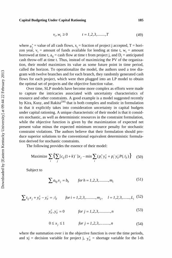
where = value of all cash flows, xj = fraction of project j accepted, T = hori-zon year, vt = amount of funds available for lending at time t, wt = amountborrowed at time t, atj = cash flow at time t from project j, and Dt = anticipatedcash throw-off at time t. Thus, instead of maximizing the PV of the organiza-tion, their model maximizes its value as some future point in time period,called the horizon. To operationalize the model, the authors used a tree dia-gram with twelve branches and for each branch, they randomly generated cashflows for each project, which were then plugged into an LP model to obtainthe optimal set of projects and the objective function value.
Over time, SLP models have become more complex as efforts were madeto capture the intricacies associated with uncertainty characteristics ofresource and other constraints. A good example is a model suggested recentlyby Kira, Kusy, and Rakita[30] that is both complex and realistic in formulationin that it explicitly takes into consideration uncertainty in capital budgetsunder capital rationing. A unique characteristic of their model is that it consid-ers stochastic, as well as deterministic resources in the constraint formulation,while the objective function is given by the maximization of expected netpresent value minus the expected minimum recource penalty for stochasticconstraint violations. The authors believe that their formulation should pro-duce superior solutions to the conventional equivalent deterministic formula-tion derived for stochastic constraints.
The following provides the essence of their model:
Subject to
where the summation over i in the objective function is over the time periods,and xj = decision variable for project j, = shortage variable for the l-th
v w t Tt t, ........,≥ =0 1,2,3, (49)
a j+
Maximize { }[ ( ) ] min ( ( )c k x p y p y Pij j i il i il iliji
1+ − +− + + − −∑∑∑ β (50)
a x b for h mhj j h= =∑ 1,2,3,........., 1(51)
t x y y for i m lij j il il il+ − = = =+ −∑ β 1,2,3, 1,2,3,.........., , .....2 ...,Li(52)
y y for j nil il+ − = =, ,...........,0 1,2,3 (53)
0 1≤ ≤ =x for j nj 1,2,3,.........., (54)
yil+
Dow
nloa
ded
by [
Eas
tern
Ken
tuck
y U
nive
rsity
] at
09:
44 2
2 Fe
brua
ry 2
013
186 Khan
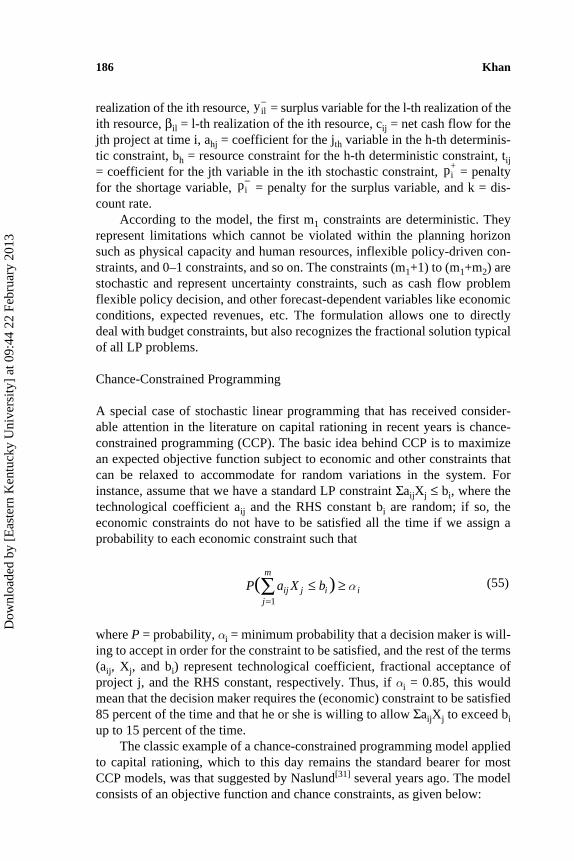
realization of the ith resource, = surplus variable for the l-th realization of theith resource, βil = l-th realization of the ith resource, cij = net cash flow for thejth project at time i, ahj = coefficient for the jth variable in the h-th determinis-tic constraint, bh = resource constraint for the h-th deterministic constraint, tij= coefficient for the jth variable in the ith stochastic constraint, = penaltyfor the shortage variable, = penalty for the surplus variable, and k = dis-count rate.
According to the model, the first m1 constraints are deterministic. Theyrepresent limitations which cannot be violated within the planning horizonsuch as physical capacity and human resources, inflexible policy-driven con-straints, and 0–1 constraints, and so on. The constraints (m1+1) to (m1+m2) arestochastic and represent uncertainty constraints, such as cash flow problemflexible policy decision, and other forecast-dependent variables like economicconditions, expected revenues, etc. The formulation allows one to directlydeal with budget constraints, but also recognizes the fractional solution typicalof all LP problems.
Chance-Constrained Programming
A special case of stochastic linear programming that has received consider-able attention in the literature on capital rationing in recent years is chance-constrained programming (CCP). The basic idea behind CCP is to maximizean expected objective function subject to economic and other constraints thatcan be relaxed to accommodate for random variations in the system. Forinstance, assume that we have a standard LP constraint ΣaijXj ≤ bi, where thetechnological coefficient aij and the RHS constant bi are random; if so, theeconomic constraints do not have to be satisfied all the time if we assign aprobability to each economic constraint such that
where P = probability, ai = minimum probability that a decision maker is will-ing to accept in order for the constraint to be satisfied, and the rest of the terms(aij, Xj, and bi) represent technological coefficient, fractional acceptance ofproject j, and the RHS constant, respectively. Thus, if ai = 0.85, this wouldmean that the decision maker requires the (economic) constraint to be satisfied85 percent of the time and that he or she is willing to allow ΣaijXj to exceed biup to 15 percent of the time.
The classic example of a chance-constrained programming model appliedto capital rationing, which to this day remains the standard bearer for mostCCP models, was that suggested by Naslund[31] several years ago. The modelconsists of an objective function and chance constraints, as given below:
yil−
pi+
pi−
P a X bij j i ij
m
( )≤ ≥=
∑ α1
(55)
Dow
nloa
ded
by [
Eas
tern
Ken
tuck
y U
nive
rsity
] at
09:
44 2
2 Fe
brua
ry 2
013
Capital Budgeting Under Capital Rationing 187
Subject to
where E = expected value operator, P = probability of the statement within theparentheses, Aj = horizon value at time T for all cash flows subsequent tothe horizon associated with project j, Xj = fraction of jth projectaccepted, r = interest rate, Vt = amount of money lent at time t at interestrate r, Wt = amount of money borrowed at time t at interest rate r, atj = cashflows associated with project j at time t, Dt = cash flows generated by otheractivities than the investment of projects with cash flows, and at = probabilityrequiring the constraint to be within the parentheses.
A couple of points are worth noting about the model formulation:The variables aij, Aj, and Di are all random. As such, it is not necessary thatthe constraint statements within the parentheses be fully satisfied. However,the decision makers may want that they be satisfied at least αi percent of thetime, and, for the remainder, allow the technological coefficient associatedwith the project to exceed the RHS constant. The problem then becomes oneof maximizing the expected value of the horizon value for all acceptedprojects, plus the amount of money lent, minus the amount of money bor-rowed at the horizon period T (Equation 56). The maximization is carried outsubject to a budget constraint expressed as a chance constraint in each periodover the planning horizon.
Although both SLP and CCP deal with uncertainty conditions, thesolution methodology for CCP is somewhat more complex than the standardstochastic programming methodologies. CCP requires the derivation of deter-ministic equivalents for all chance constraints by taking into consideration theshape and parameters of the probability distributions of all random variables.The derivation often produces non-linear equations, which can greatly compli-cate the feasibility of the solution. Finding the ‘deterministic equivalents’ is
Maximize E A X V Wjj
m
j T T( )=
∑ + −1
(56)
E A X V W Djj
m
j T( )=
∑ ∑+ − ≤ ≥1
1 1 1α (57)
P a X V r W r V W D tij j i i t t i ti
t
i
t
i
t
j
m
i
t
( )− + + − ≤ ≥==
−
=
−
==∑∑∑∑∑ α
11
1
1
1
11
== 1,2,3,.......,T
(58)
0 ≤ ≤ ≥X 1 V 0bj tW (59)
Dow
nloa
ded
by [
Eas
tern
Ken
tuck
y U
nive
rsity
] at
09:
44 2
2 Fe
brua
ry 2
013
188 Khan
more involved and is nicely illustrated by Charnes and Cooper,[32] Byrneet al.,[33] Lee et al.,[34] and others.
Hillier[35] offered a two-stage solution algorithm for chance-constrainedprogramming that is more flexible than the conventional methods in that thedecision variables could be either bounded and continuous, or restricted to beeither 0 or 1 (as when “yes” or “no” decision must be made), and where someor all of the parameters are random variables that may be statistically dependent.De et al.[36] take it a step further by providing a chance-constrained formula-tion for a 0–1 goal programming problem where the technological coefficientsare stochastic. The model is really an extension of the works by Keown andMartin,[37] and Keown and Taylor,[38] but solved by utilizing Naslund’sapproximation for converting the non-linear part of the deterministic equiva-lent to a linear part, and an algorithm developed by Lee and Morris[39] for theGP component of the problem.
An important characteristic of the CCP models involving capital rationingis that much of their application is based on the assumption of a decision envi-ronment that is precise with well-defined parameters. But CCP can also beused in situations where the decision environment is imprecise or fuzzy, asmost government decision environments are. Liu and Ishwara[40] provide aninteresting framework, where they introduce fuzzy parameters to solve achance-constrained problem in a fuzzy environment. They further update themodel to integer case to make it more suitable for capital rationing problemsin a fuzzy environment.[41]
The following provides the basic structure of their model:
Subject to
where Pr{hixi ≥ ξI I} ≥ ai with i=1,2,3,.........,n are separate chance constraints,which can be easily replaced, if needed, by a joint form Pr{hixi ≥ ξI I} ≥ ai orsome mixed forms. An interesting aspect of the model is that it can be easilyintegrated to a multi-objective decision making problem with assigned target
Maximize c x c x c xn n1 1 2 2+ + +......... (60)
a1 1 2 2x a x a x an n+ + + ≤........ (61)
b x b x b x bn n1 1 2 2+ + + ≤......... (62)
Pr 1,2,3,1{ } .........,η ξi i ix a i n≥ ≥ = (63)
x i ni , ........., ,= 1,2,3, non-negative integers (64)
Dow
nloa
ded
by [
Eas
tern
Ken
tuck
y U
nive
rsity
] at
09:
44 2
2 Fe
brua
ry 2
013
Capital Budgeting Under Capital Rationing 189
levels and priority structure set by the decision makers, and formulated as astochastic goal programming (SGP) model.
Recent studies on CCP have focused on a diverse range of issues. Forinstance, a study by Gao et al.[42] addresses the capital rationing problem withfuzzy decisions by offering a hybrid intelligent algorithm to solve theproblem. Another study by Sarper[43] challenges the universality of the nor-mally distributed random variables and suggests the usefulness of alternativeforms such as uniformly distributed variables since uniform distributions canbe easily approximated into normal distributions. A more recent study by Gurgurand Luxhoj[44] looks at capital rationing with the selection of the best capitalproject mix when cash flows and available budgets are asymmetrically distrib-uted random variables. For this, they use the Weibull distribution, since, undercertain circumstances, it can better approximate many observable phenomenathan the normal distribution. And unlike the normal distribution, it does nottake negative values.
Quadratic Programming
Quadratic programming (QP) is another special case of mathematical pro-gramming that has been applied to capital rationing problems under uncer-tainty, where the goal is to maximize a quadratic objective function subject toa set of linear constraints. The QP models are much easier to solve than thenon-linear programming models, because the feasible region is convex(curved outward in a two-dimensional plane). Convexity ensures that a localoptimal solution is also the global optimal solution, meaning that any feasiblesolution that maximizes the objective function over the feasible solution alsomaximizes it over the entire set of feasible solutions. What this means in oper-ational terms is that one only needs to find one local optimum, instead of aninfinite number of local optima, to reach the global optimum.
The earliest QP model applied to capital rationing was by Farrar,[45] whoextended the works of Markowitz,[46] and Weingartner[6] by incorporating inthe objective function both a project’s expected NPV and its variance. Thegeneral QP formulation, as suggested by Farrar, can be expressed as follows:
Subject to
Maximize Z X U A X Xjj
m
j ij
m
i
n
j ij= −= ==
∑ ∑∑1 11
σ (65)
X jj
m
=∑ =
1
1(66)
Dow
nloa
ded
by [
Eas
tern
Ken
tuck
y U
nive
rsity
] at
09:
44 2
2 Fe
brua
ry 2
013
190 Khan
where Xj = proportion of total budget invested in project j, Uj = expected NPVof project j, A = average coefficient of risk aversion, sij covariance betweenthe NPV of project i and project j (but if i=j, it becomes the variance of theproject j).
The objective of the model is to maximize the expected utility, whichincludes both mean and variance of all possible portfolios, and a risk aversioncoefficient, A. The formulation allows for trade-offs between risk and return,as well as the interactions between all possible pairs of investment projects,but yields a minor solution problem because of the inclusion of the decisionvariables that are continuous. The problem can be overcome, however, iftreated as an integer QP problem, as Mao and Wallengford[47] has demon-strated with an integer solution using the traditional branch-and-boundalgorithm.
Thompson[48] offered another approach that addresses a single-period QPproblem capable of dealing with competitive, as well as complimentaryprojects, but found the programming approach somewhat limiting when deal-ing with multi-period modeling. In another study, McBride[49] modified theMarkowitz’ model, which provided the ground work for early quadratic pro-gramming problems, by offering a solution procedure that can be used withany algorithm to solve 0–1 quadratic rationing problems. Recently, Rosenblattand Sinuany-Stern[50] have suggested a procedure that deals with two objec-tive functions, instead of one-one maximizing the present value of acceptedprojects and the other minimizing their risks. Although risk is less of a prob-lem in government than uncertainty, one can easily substitute it for uncer-tainty conditions.
The following provides the basic structure of their model:
Subject to
where pj = the expected present value of project j, vj = the variance of projectj, sj = the first period expected cash outflow of project j, S = budget availablefor allocation to all projects at time 1, xj = decision variable, equals 1 if project
X 0j ≥ (67)
Maximize ( )( )α αp x v xj j jj
n
j
n
j− −==
∑∑ 111
(68)
s x j nj jj
n
≤ ==
∑ S 1,2,31
,.........,(69)
x 0 1j or= (70)
Dow
nloa
ded
by [
Eas
tern
Ken
tuck
y U
nive
rsity
] at
09:
44 2
2 Fe
brua
ry 2
013
Capital Budgeting Under Capital Rationing 191
j is accepted and 0 otherwise, a = weight assigned to project’s present value(with corresponding weight to the variance is (1-a), where 0 ≤ a ≤ 1, and n =number of projects considered.
A more recent study by Chardaire and Sutter[51] uses a mixed-integer qua-dratic programming approach, where they, first, use the traditional branch-and-bound algorithm to find the minima of the quadratic function, then, use aLagrangian decomposition method (used in partitioning an initial function intosub-functions) to find the solution for the quadratic rationing problem. Themethod, according to the authors, should produce better results in practice.
Another recent study with potential for use in capital rationing problem ingovernment is by Jackson and Staunton,[52] where the authors describe twoapplications of quadratic programming, one from the early years of Markowitzand the other a more recent innovation based on the work of Sharpe. Theinteresting thing about their model is that it uses Excel’s Solver to find theoptimal weights for both quadratic programming applications. They also use adirect analytic solution for generating the efficient frontier where there are noinequality constraints using the matrix functions in Excel. The study opens upnew opportunities for solving complex optimization problems with standardspreadsheets, although they have been used for a long time for small-scaleproblems.[53]
SUMMARY AND CONCLUSION
This article has presented a brief overview of optimization models in capitalrationing under both certainty and uncertainty conditions. Three types of modelswere discussed under certainty conditions—linear, integer, and goalprogramming. Similarly, three types of models were discussed under uncer-tainty conditions—Monte Carlo simulation, stochastic linear programming,and quadratic programming. It is impossible to summarize all the works thatbeen done on the subject, almost all of which are for for-profit organizations;nevertheless, the paper provides a glimpse of the potential these models havefor capital rationing problems in government.
REFERENCES
1. Man, J. C. T. (1966). The internal rate of return as a ranking criterion. TheEngineering Economist, 12(2), 1–3.
2. Tarimcilar, M. M. and Khaksari, S. Z. (1991). Capital budgeting in hospi-tal management using the analytic hierarchy process. Socio-EconomicPlanning Sciences, 25(1), 27–34.
3. Khan, A. (1997). Capital rationing, priority setting, and budget deci-sions: An analytical guide. In R. T. Golembiewski and J. Rabin (eds.),
Dow
nloa
ded
by [
Eas
tern
Ken
tuck
y U
nive
rsity
] at
09:
44 2
2 Fe
brua
ry 2
013
192 Khan
Public budgeting and finance, 4th Edition. New York: Marcel Dekker,963–974.
4. Lorie, J. H. and Savage, L. J. (1955). Three problems in rationing capital.The Journal of Business, 28(2), 229–239.
5. Charnes, A., Cooper, W. W., and Miller, M. H. (1959). An application oflinear programming in financial budgeting and the cost of funds. TheJournal of Business, 32(1), 20–46.
6. Weingartner, H. M. (1963). Mathematical programming and the analysisof capital budgeting problems. Englewood-Cliffs, NJ: Prentice Hall.
7. Fabozzi, F. J. (1978). A Portfolio approach to capital budgeting:An application. The Journal of the Operations Research Society, 29(3),245–249.
8. Bhaskar, K. (1978). Linear programming and capital budgeting: Thefinancing problems. Journal of Business Finance and Accounting, 5(2),159–194.
9. Rychel, D. F. (1977). Capital budgeting with mixed integer linear pro-gramming: An application. Financial Management, 6(4), 11–19
10. Benjamin, C. O. (1985). A linear goal programming model for public-sector project selection. The Journal of the Operations Research Society,36(1), 13–23.
11. Aggarwal, R. (1994). Capital budgeting under uncertainty. Journal ofFinance, 49(2), 747–750.
12. Charnes, A. and Cooper, W. W. (1961). Management models and indus-trial applications of linear programming, Volumes I and II. John Wileyand Sons, New York.
13. Ijiri, Y. (1965). Management goals and accounting for control. Amsterdam:North-Holland Publishing Company.
14. Lee, S. M. (1972). Goal programming for decision analysis. Philadelphia:Auerbach Publishing Company.
15. Ignizio, J. P. (1976). Goal programming and extension. Lexington Books,Lexington.
16. Lee, S. M. (1979). Goal programming methods for multiple objectiveinteger programs. Atlanta. American Institute of Industrial Engineers.
17. Taylor, B. W. III, Keown, A. J., and Greenwood, A. G. (1983). An integergoal programming model for determining military aircraft expenditures.The Journal of the Operations Research Society, 34(5), 379–390.
18. Markland, R. E. and Vickerey, S. K. (1986). The efficient computerimplementation of a large-scale goal programming model. EuropeanJournal of Operations Research, 26(3), 341–354.
19. Lee, S. M. and Luebbe, R. L. (1987). A zero-one goal programming algo-rithm using partitioning and constant aggregation. The Journal of theOperations Research Society, 38(7), 633–641.
20. Zeleny, M. (1981). The pros and cons of goal programming. Computersand Operations Research, 8(4), 357–359.
Dow
nloa
ded
by [
Eas
tern
Ken
tuck
y U
nive
rsity
] at
09:
44 2
2 Fe
brua
ry 2
013
Capital Budgeting Under Capital Rationing 193
21. Hallefjord, A. and Jornsten, K. (1988). A critical comment on integer goalprogramming. The Journal of the Operations Research Society, 39(1),101–104.
22. Ignizio, J. P. (1989). On the merits and demerits of integer goal program-ming. The Journal of the Operations Research Society, 40(8), 781–785.
23. Steuer, R. E. Multicriteria optimization: Theory, computation, and appli-cation. New York: John Wiley and Sons.
24. Hertz, D. (1964). Risk analysis in capital investment. Harvard BusinessReview, 42(1), 95–106.
25. Groff, G. K. and Muth, J. F. (1972). Operations management: Analysisfor decisions. Homewood, IL: Richard D. Irwin.
26. Lewllen, W. G. and Long, M. S. (1972). Simulation vs. single-value esti-mates in capital expenditure analysis. Decision Sciences, 3(4), 19–33.
27. Kryzanowski, L., Lustig, P., and Schwab, B. (1972). Monte-Carlo simula-tion and capital expenditure decisions — A case study. The EngineeringEconomist, 18(1), 31–48.
28. Shannon, R. E. (1975). System simulation: The art and science.Englewood-Cliffs, NJ: Prentice-Hall.
29. Salazar, R. C. and Sen, S. K. (1968). A simulation of capital budgetingunder uncertainty. Management Science, 15(1), 161–179.
30. Kira, D. S. Kusy, M. I., and Rakita, I. (2000). The effect of project risk on cap-ital rationing under uncertainty. The Engineering Economist, 45(1), 37–55.
31. Naslund, Bo. (1966). A model of capital budgeting under risk. Journal ofBusiness, 39(2), 257–271.
32. Charnes, A. and Cooper, W. W. (1963). Deterministic equivalents foroptimizing and satisficing under chance constraints. OperationsResearch, 11(1), 18–39.
33. Byrne, B, Cooper, W. W., and Korteneck, K. (1967). A chance-constrained programming approach to capital budgeting with portfoliotype payback and liquidity constraints and horizon positive controls.Journal of Financial and Quantitative Analysis, 2(4), 339–364.
34. Lee, S. M., Moore, L. J., and Taylor, B. W. (1990). Management science,Boston MA: Allyn and Bacon.
35. Hillier, F. B. (1967). Chance-constrained programming with 0–1 or boundedcontinuous decision variables. Management Science, 14(1), 34–57.
36. De, P. K., Acharya, D., and Sahu, K. C. (1982). A chance-constrainedgoal programming model for capital budgeting. The Journal of the Opera-tions Research Society, 33(7), 635–638.
37. Keown, A. J. and Martin, J. D. (1976). An integer goal programmingmodel for capital budgeting in hospitals. Financial Management, 5(3),28–35.
38. Keown, A. J. and Taylor, B. W. (1980). A chance-constrained integergoal programming model for capital budgeting in the production area.The Journal of the Operations Research Society, 31(7), 579–589.
Dow
nloa
ded
by [
Eas
tern
Ken
tuck
y U
nive
rsity
] at
09:
44 2
2 Fe
brua
ry 2
013
194 Khan
39. Lee, S. M. and Morris, R. (1977). Integer Goal Programming methods. InM. Starr and M. Zeleny (eds) Multiple criteria decision making. Amster-dam: North-Holland Publishing Company, 273–289.
40. Liu, B. and Iwamura, K. (1998). Chance-Constrained programming withfuzzy parameters. Fuzzy Sets and Systems, 94(2), 227–237.
41. Iwamura, K. and Liu, B. (1998). Chance-Constrained integer program-ming models for capital budgeting in fuzzy environments. The Journal ofthe Operations Research Society, 49(8), 854–860.
42. Gao, J. W., Zhao, J. H., and Ji, X. Y. (2005). Fuzzy chance-constrainedprogramming for capital budgeting problem with fuzzy decisions. FuzzySystems and Knowledge Discovery, Pt.1, Proceedings of the LectureNotes in Artificial Intelligence, 304–311.
43. Sarper, H. (1993). Capital rationing under risk: A chance-constrainedapproach using uniformly distributed cash flows and available budgets.The Engineering Economist, 39(1), 49–76.
44. Gurgur, C. Z. and Luxhoj, J. T. (2003). Application of chance-constrainedprogramming to capital rationing problems with asymmetrically distrib-uted cash flows and available budgets. The Engineering Economist,48(3), 241–258.
45. Farrar, D. F. (1962). The investment decision under uncertainty. Engle-wood-Cliffs, NJ: Prentice-Hall.
46. Markowitz, H. (1952). Portfolio selection. Journal of Finance, 7(1),77–91.
47. Mao, J. C. T. and Wallinford, B. A. (1968). An extension of Lawler andBell’s Method of Discrete Optimization. Management Science, 15(2),51–61.
48. Thompson, H. E. (1976). Mathematical programming, the Capital AssetPricing Model, and capital budgeting of interrelated projects. The Journalof Finance, 31(1), 125–131.
49. McBride, R. D. (1981). Finding the integer efficient frontier for quadraticcapital budgeting problems. The Journal of Financial and QuantitativeAnalysis, 16(2), 247–253.
50. Rosenblatt, M. J. and Sinuany-Stern, Z. (1989). Generating the discreteefficient frontier to the capital budgeting problem. Operations Research,37(3), 384–394.
51. Chardaire, P. and Sutter, A. (1995). A decomposition method for qua-dratic zero-one programming. Management Science, 41(4), 704–712.
52. Jackson, M. and Staunton, M. D. (1999). Quadratic programming appli-cations in finance using Excel. The Journal of the Operations ResearchSociety, 50(12), 1256–1266.
53. James, K. H. (1987). Linear and dynamic programming with Lotus 1-2-3.Release 2. Portland, OR: Management Information Source, Inc.