The University of Manchester Research

Carbon dioxide emission and bio-capacity indexing fortransportation activitiesDOI:10.1016/j.jenvman.2018.06.010

Document VersionAccepted author manuscript

Link to publication record in Manchester Research Explorer

Citation for published version (APA):Labib, S., Neema, M. N., Rahaman, Z., Patwary, S. H., & Shakil, S. H. (2018). Carbon dioxide emission and bio-capacity indexing for transportation activities: A methodological development in determining the sustainability ofvehicular transportation systems. Journal of Environmental Management, 223, 57-73.https://doi.org/10.1016/j.jenvman.2018.06.010Published in:Journal of Environmental Management

Citing this paperPlease note that where the full-text provided on Manchester Research Explorer is the Author Accepted Manuscriptor Proof version this may differ from the final Published version. If citing, it is advised that you check and use thepublisher's definitive version.

General rightsCopyright and moral rights for the publications made accessible in the Research Explorer are retained by theauthors and/or other copyright owners and it is a condition of accessing publications that users recognise andabide by the legal requirements associated with these rights.

Takedown policyIf you believe that this document breaches copyright please refer to the University of Manchester’s TakedownProcedures [http://man.ac.uk/04Y6Bo] or contact uml.scholarlycommunications@manchester.ac.uk providingrelevant details, so we can investigate your claim.

Download date:16. Feb. 2022

1

Title Page

Carbon dioxide Emission and Bio-capacity indexing for transportation

activities: A methodological development in determining the

sustainability of vehicular transportation Systems

S M Labib a*; Dr. Meher Nigar Neema b; Zahidur Rahaman c; Shahadath

Hossain Patwary d; Shahadat Hossain Shakil e

Corresponding Author:

S M Labib*

a PhD Researcher, School of Environment, Education and Development (SEED), University

of Manchester.

Email: sm.labib@manchester.ac.uk

Arthur Lewis building (1st Floor); Oxford Road; Manchester; M13 9PL

Co-authors:

b Professor, Department of urban and regional planning, Bangladesh University of Engineering

and Technology (BUET). E-mail: mnneema@yahoo.com

c Sub-Registrar, Ministry of Law, Justice and Parliamentary Affairs, Government of

Bangladesh. Email: abeer.urp@gmail.com

d Assistant Urban Planner, Sheltech (Pvt.) Ltd. Email: shahadath3.1416@gmail.com

e Project Management Specialist (Environment), Economic Growth Office, USAID.

U.S. Agency For International Development, American Embassy, Madani Avenue. Dhaka-

1212.

Email: sshakil@usaid.gov

2

Abstract

CO2 emissions from urban traffic are a major concern in an era of increasing ecological

disequilibrium. Adding to the problem net CO2 emissions in urban settings are worsened due

to the decline of bio-productive areas in many cities. This decline exacerbates the lack of

capacity to sequestrate CO2 at the micro and meso-scales resulting in increased temperatures

and decreased air quality within city boundaries. Various transportation and environmental

strategies have been implemented to address traffic related CO2 emissions, however current

literature identifies difficulties in pinpointing these critical areas of maximal net emissions in

urban transport networks. This study attempts to close this gap in the literature by creating a

new lay-person friendly index that combines CO2 emissions from vehicles and the bio-capacity

of specific traffic zones to identify these areas at the meso-scale within four ranges of values

with the lowest index values representing the highest net CO2 levels. The study used traffic

volume, fuel types, and vehicular travel distance to estimate CO2 emissions at major links in

Dhaka, Bangladesh’s capital city’s transportation network. Additionally, using remote-sensing

tools, adjacent bio-productive areas were identified and their bio-capacity for CO2

sequestration estimated. The bio-productive areas were correlated with each traffic zone under

study resulting in a Emission Bio-Capacity index (EBI) value estimate for each traffic node.

Among the ten studied nodes in Dhaka City, nine had very low EBI values, correlating to very

high CO2 emissions and low bio-capacity. As a result, the study considered these areas

unsustainable as traffic nodes going forward. Key reasons for unsustainability included

increasing use of motorized traffic, absence of optimized signal systems, inadequate public

transit options, disincentives for fuel free transport (FFT), and a decline in bio-productive areas.

Key words: Carbon dioxide (CO2) Emission, Transportation Sustainability Rating, Bio-

Capacity, Urban Transport, Low carbon transport.

3

1. Introduction

Urban transportation produces significant amounts of overall carbon dioxide (CO2)

emissions in urban areas (Li, 2011). Given an era of global warming and climate change,

controlling CO2 emissions, in support of sustainable development is a major concern in

maintaining overall global sustainability and livability. According to the International Energy

Agency (IEA),the transportation sector of the global economy was the second highest sectoral

emitter of CO2 emissions in year 2008; accounting for 22% of global CO2 emissions (Loo and

Li, 2012). Urban areas of the global economy with 54.5% (rising to 60% by 2030) of the global

population are responsible for 75% of global CO2 emissions, and intra-urban transportation

contributed 17.5% of those CO2 emissions (Fan and Lei, 2016). Dodman (2009), noted that,

major cities around the world produced massive amounts of CO2 from daily traffic movements.

CO2 emissions in representative cities such as: London (22 percent), New York (23 percent),

Toronto (36 percent), and São Paulo (59.7%) support Dodman’s observations. Additionally,

fast developing countries with large populations such as India and China, are now experiencing

steadily intensifying emissions of CO2 from their burgeoning transportation sectors (Li, 2011;

Dodman, 2009). It has long been projected that increasing traffic movements induced globally

by both growth and increases in prosperity would be likely to increase transportation CO2

emissions if energy consumption based on fossil fuels is not reduced (Li, 2011). Therefore, low

CO2 emissions and sustainable transportation initiatives are rising in importance in global

agendas related to climate along with initiatives to change energy consumption patterns and

production paradigms.

In addition to an ongoing global increase in transportation induced CO2 emissions from

urban areas, previous studies have identified a decline in bio-productive areas in cities, due to

both a loss of area and both losses and degradation of vegetation in the remaining bio-

productive area. Researchers have explored this reduction in bio-capacity, and concurrent

increases in greenhouse gas (GHG) emissions (primarily CO2) which jointly result in a

widening deficit between the ecological footprint and bio-capacity, in turn resulting in a lack

of environmental sustainability going forward (Mancini et al., 2016; Niccolucci et al., 2012).

In a transport context, this can be a major indicator of the ability to maintain sustainability

going forward. Several studies have linked transportation and CO2 emissions; for example Shu

and Lam (2011) studied traffic related CO2 emissions and found spatial variations in

CO2 emissions from traffic activities correlated to differences in traffic intensity. Fan and Lei

(2016), analyzed CO2 emissions from traffic with a multivariate generalized Fisher index (GFI)

4

decomposition model to examine the relation between energy structure, intensity and traffic

turn-over. Zahabi et al. (2012) explored the effect of the built-environment on urban transport

emissions. Labib et al. (2013) investigated the ecological footprint of urban transportation at

city scale. Most of the existing transport-environment studies illustrated that growing

populations, and the resulting demand for transportation when combined with a lack of

available public transportation, influxes of new private vehicles to urban areas and a lack of

energy efficient vehicles contributed to increases in CO2 and other pollutant emissions

(Perveen et al., 2017; Fan and Lei, 2016; Yigitcanlar and Kamruzzaman, 2014).

Currently, in the extant literature there is a paucity of research that studies specific

locations, zones, and routes within urban transportation systems particularly those areas with

high net CO2. However, these same areas are those that would appear to require the most urgent

near-term attention from policy-makers, to formulate and implement effective strategies for

local CO2 emissions reduction. This is a matter of particular urgency due to the ongoing decline

of micro-climatic conditions in such areas as well as the need to address the decline in the

already limited extent of bio-productive areas in cities (Shakil et al., 2014). Most often,

transportation related studies have, in past, focused on mobility, accessibility, speed, or shifts

in transport modes (Kamruzzaman et al., 2015). However, these studies do not provide data

on existing conditions related to traffic related pollution as defined by net GHG emissions at

particular locations. Nor do they provide data on co-located bio-productive areas with the

capacity to diffuse or absorb emissions from local traffic.

Available ecological footprint studies at local scale (e.g. city or neighborhood level)

have provided gross estimations of CO2 emissions from residential energy, food, waste

generation and fuel consumption, and compared these with area based bio-capacities (Shakil

et al., 2014; Minx et al., 2006). However, such studies do not focus on the particulars of

transportation related problems. Such studies have measured overall fuel consumption for

transportation movements, without either breaking down transportation movements by types

or making specific transportation related recommendations to improve transportation

sustainability. Hence, there is a gap in the current literature in terms of understanding how

traffic related carbon emissions correlate with local available bio-capacity particularly on the

specific transportation routes or given zones in cities that have the highest net levels of CO2.

In order to potentially create real world scenarios that implement sustainable

transportation strategies, characterized by low CO2 emissions and full carbon sequestration, it

will be required to understand currently existing conditions related to CO2 emissions from

5

traffic as well as current carbon sequestration capacity. To facilitate such understanding the

present study has rigorously utilized traffic volume and image-based remote sensing

technologies to identify traffic zones which are critical, i.e. very heavily loaded, traffic nodes

adjacent to bio-productive areas wherein the traffic zones are defined as the area within a 500

metre radius of the critical traffic node as areas of interest (AOI). This study measured net CO2

emissions from transportation activities/movements in these AOIs utilizing an inventory based

carbon estimation methodology (Iqbal et al., 2016). The study specifically focused on the

meso-scale level of analysis, in order to gain detailed insight into the differing characteristics

of transport movement at study identified AOIs.

The present study presents a new index specifically created to correlate CO2 emissions

at critical traffic nodes with adjacent bio-capacity within the studied AOIs in order to calculate

a net CO2 emission value. This quantitative index will provide an opportunity to compare CO2

emissions with sequestration capacity at specific locations in transport networks. In aggregate,

data generated by applying this index to each critical node in a transport network will provide

further data supporting policy and remediation both in real-time and as part of computer-

simulations of ‘what-if’ scenarios. Furthermore, changes in the index values for a location

based on either changes in traffic composition or changes in local vegetation will allow policy

makers to easily grasp the effect of changes to environmental parameters which will, in turn,

allow them to correlate index values to any costs of changing traffic or environmental

parameters allowing for easier cost-benefit calculations.

2. Materials and Methods

2.1 Conceptual Design of “Emission, Bio-Capacity Index (EBI)”

Calculation of EBI values requires two types of activities; the first is related to the

determination of CO2 emissions from different vehicle types, based on different levels of

activity, fuel type and emissivity (Fig 1). EBI calculations determine the total daily and yearly

CO2 emissions from vehicular traffic activities for a given area AOI, and converts the yearly

CO2 emission value into the equivalent carbon uptake land measure (C, in global hectare)

(Wiedmann and Barrett, 2010). The second type of activity requires determining the land cover

types within the AOI and finding the corresponding bio-capacity for each land cover type.

Index values are then generated by dividing the carbon uptake land estimated from yearly

traffic CO2 emissions by the total bio-capacity of the AOI, thus providing the value for the EBI

6

for that AOI (Fig 1). This relatively simple index combines the emissions of CO2 emissions

from traffic in a given area and co-located bio-capacity at the meso-scale into a single value.

The basis of the model was derived from the concept of ecological footprints, and their

relationship with biological capacities (Mancini et al., 2016; Ontl and Schulte, 2012;

Wiedmann and Barrett, 2010).

The index developed for the present study is a new approach to providing tools that are

easily and quickly comprehensible to policy-makers and non-experts and which will assist in

determining the sustainability of a given transportation network as defined by net GHG

emissions. Thus, this index will provide a sustainability-rating system for given locations

and/or zones within a transportation network. Previously transportation networks’ ecological

footprints have been estimated by researchers; however combining the ecological footprint

with co-located bio-capacity has heretofore only been explored in non-transport sectors such

as housing, food and energy consumption (Nakajima and Ortega, 2016; Moore et al., 2013).

[Figure 1 Near Here]

2.2 Case Study Area

In order to conduct the present study of traffic-related CO2 emissions and co-located

carbon sequestration capacity, a detailed spatial extent was selected. The present study was

conducted at meso-scale, at ten major intersections (nodes) within the transportation network

of Dhaka. Dhaka, is one of the fastest growing mega-cities globally and a major area of urban

agglomeration. As a result, the city generates millions of trips every day, and traffic activity is

both intense and intensifying (Iqbal et al., 2016). A complex network of roads of varied

capacity, growing demands for private vehicles, and overall increase in motorization from year

to year due to better economic growth and prosperity, are driving commensurate increases in

CO2 emissions. Dhaka’s major arteries are characterized by chronic traffic congestion further

exacerbating fuel consumption and related CO2 emissions (Labib et al., 2013; Karim, 1999).

In addition to traffic emissions, the city is experiencing a loss of bio-productive areas

capable of sequestering CO2 emissions. Dewan and Yamaguchi (2009) found that the city was

changing its land cover types, and built up areas were increasing with concomitant decreases

in vegetation, bodies of water and fallow land (Hassan and Southworth, 2017; Dewan and

Yamaguchi, 2009). For example, in the period from 1999 to 2009 built up areas within Dhaka

increased by 16.86% of the total urban area, while vegetative cover, bodies of water and fallow

7

land decreased by 3.23%, 1.98% and 10.80% respectively (Ahmed and Ahmed, 2012). Each of

these declines could also be understood as a decline in available bio-productive areas. Thus,

the continuing increases in CO2 emissions combined with decreases in capacity to sequestrate

carbon within city boundaries are resulting in continual increases in net CO2 generation (Labib

et al., 2013).

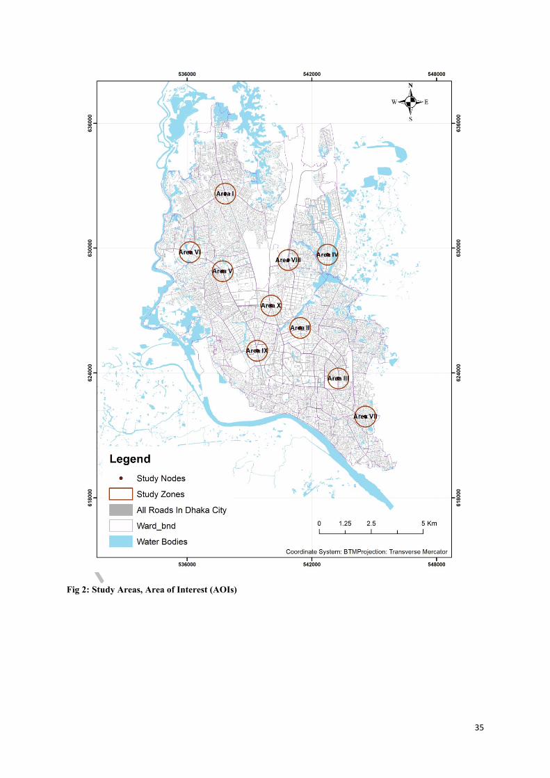
The ten study zones selected for the present study are major nodes in Dhaka’s urban

transportation network. The researchers delineated a buffer of one half of a kilometer radius

around each node to create study zones/AOIs that allowed explicit determination of the spatial

domain of measurement. The sites selected were: Mirpur 10 no., Technical Morh, Shymoli,

Framgate, Mohakhali, Gulshan 1, Mog bazaar, Science lab, Motijheel and Jatrabari (Fig 2).

While city-level macro scale studies (Labib et al., 2013) can provide a general overview of

overall emissions and extant bio-capacity, they are lacking in the specificity and detail required

for meso-level analysis (Iqbal et al., 2016; Dias et al., 2016). Therefore, the present study

focused on specific sites for detailed examination of GHG emissions as well as associated bio-

capacity. Study site selection was focused on traffic nodes characterized by high levels of

traffic volume, connectivity and diverse trip type generation. (Labib et al., 2014).

[Figure 2 Near Here]

2.3 Vehicular Emission Estimation method

2.3.1 Emission Modeling

In order to determine the amount of CO2 emitted due to vehicular activity in Dhaka at

selected AOIs; an inventory based emission model was utilized based on vehicular travel within

the AOIs. In such models “bulk” emission factors (emissivity) and vehicle activity (distance

travelled) are considered in determining an emission level from each different class of vehicles.

This creates an aggregate, top-down, approach to estimating transport related CO2 emissions

(Kamruzzaman et al., 2015; Wadud and Khan, 2011; Afrin et al. 2012). The specific model

that was utilized to estimate carbon dioxide emissions is given in eq1 (Pan et al., 2016;

Kamruzzaman et al., 2015; Neema and Jahan, 2014).

𝐸𝑖 = ∑ ∑ 𝐸𝐹𝑖𝑗𝑘𝑛𝑘=1 𝐴𝑗𝑘

𝑛𝑗=1 (eq1)

Where,

i = Type of a pollutant (in this case CO2)

8

j = Fuels consumed (e.g. CNG, Gasoline)

k = Emitting Vehicular type (Volume survey)

Ei = Emissions from pollutant

EFijk = Emission Factor (g/km)

Ajk =Activity level for each pollutant source.

The activity level for each pollutant source within a particular study site has been determined

by the following relationship in eq2;

𝐴𝑗𝑘 = 𝑉𝐾𝑇 = 𝐿 × 𝐴𝐴𝐷𝑇 (eq2)

Where,

Ajk = Activity level for each pollutant source for each study area (km/day)

VKT = Vehicle Kilometers Traveled (km/day).

L = Road length (km) of the selected links within the study area

AADT = Annual Average Daily Traffic (traffic volume/day)

2.3.2 Vehicle Kilometers Traveled (VKT)

The three methodological processes typically used to measure CO2 emissions in

aggregate, top-down, approaches to emissions modeling, are: (i) fuel consumption, (ii) specific

vehicle tagging/tracking, or (iii) travel distance methods (e.g. VKT). In the present study

vehicle activity level was determined by measurement of VKT, the most widely used method

in determining CO2 emissions at meso or micro scales (Kamruzzaman et al., 2015; Iqbal et al.,

2016). For each study area, the selected road links’ lengths were determined using GIS data for

the Dhaka city traffic network drawn from the Detailed Area Plan database, developed by

RAJUK, the city development authority. The present study made the assumption that, once a

vehicle entered the study zone, and traveled the zone’s road links, that this travel represented

their total distance or VKT within the AOI zone(s).

2.3.3 Vehicle Fuel Usage Type

Emission levels and emissions factors for each vehicle type depend on the fuel usage

as well as fuel types consumed by that particular type of vehicle (Andrews, 2008). The emission

estimation model suggests that while fuel usage is a factor of major significance in determining

the total amount of emissions, the type of fuel a vehicle consumes during the process of

9

combustion also impacts on the levels of CO2 emitted. Thus, for the present study a detailed

database summarizing the type of fuel used by each different type of vehicle found in the

present study was necessary. Table 1 presents the fuel types each class of vehicle found in the

present study could use and the percentage of use of each fuel type within each vehicle class.

The table also correlates the fuel type usages for each vehicle class with the grams per kilometer

of CO2 emitted (Neema and Jahan, 2014; Wadud and Khan, 2011).

The specific fossil fuel types identified in Table 1 are: diesel, gasoline (petrol) and

compressed natural gas (CNG). Among different vehicle classes, 100% of motorcycles

observed used only gasoline, while 100% of all auto rickshaws, taxi cabs, and legunas (a

partially open microbus converted to increase capacity) observed in the AOIs used CNG. A

comparison of fuel usage values shows that CNG is the most used fuel amongst all vehicle

classes in Dhaka due to the wide availability of natural Gas within Bangladesh.

[Table 1 Near Here]

2.3.4 Emissivity of various vehicles based on different fuel types

In the inventory based emission model, emissivity represents per unit emissions

expressed in grams per kilometer of vehicle travel (gm/km) (Pan et al, 2016; Kamruzzaman et

al., 2015). In order for the emissions model to provide valid results it requires the emission

factors (EFs) to be accurately measured. Studies conducted by: Labib et al., (2013), and Neema

and Jahan, (2014) of Dhaka’s transport network used emission factors developed by Wadud

and Khan (2011) and showed that these EFs do provide acceptable level of accuracy for

emissions from vehicles, operating under typical traffic conditions in Dhaka. Table 1 presents

the corrected emission factors correlated with the relevant different vehicles categories and fuel

types. It should be noted that, table 1 shows that for some vehicle classes (e.g. buses and jeeps)

have higher emission factors associated with combustion of CNG compared to diesel or petrol.

However, most vehicle classes (e.g. cars, micro-buses, pickups) had lower values for their

emissions factors when fueled with CNG compared to diesel and petrol. The researchers note,

that the efficiency of internal combustion engines under varying fuel regimes is a complex

topic impacted by many factors beyond the scope of this study and further note that both the

potential quality of liquid fuel to CNG conversions (Diesel-to-CNF, Petrol-to-CNG) and

overall vehicle maintenance are impacted by both parts availability and economic constraints

that many vehicle operators in developing countries face (Wadud and Khan, 2011).

10

Overall, the researchers suggest that it may be argued that these EFs are an estimate of

per-unit emissions for different modes where the vehicles involved are at least likely to have

reached normal engine operating temperatures. They also note that different per-unit emission

values might be calculated if all factors including: fuel efficiency, engine type, age of vehicle,

quality of engine conversion from liquid to CNG fuel, and hot/cold emission values could be

provided for detailed emissions modeling. However, failing the ability to do such data-intense

modeling, and in light of the fact that the emissions data gathered by the current study was

analyzed utilizing empirically based values for Dhaka emissions from the Wadud and Khan

(2011), where they estimated and validated the EFs for the vehicle classes by their field

observation and tests. The researchers are confident that EF values derived for vehicular

emissions for this study represent values based on the real world traffic composition found in

Dhaka by taking account of vehicle condition, fuel use and vehicle efficiency in terms of traffic

operation in Dhaka.

Furthermore, as the presents study was focused on the meso-scale and based on the

aggregate method of data collection, The EF values used were a necessary compromise to cover

larger volume of traffic in the major streets of Dhaka city. Therefore, intensive emission

modelling (usually micro-scale) was not adopted in this case study, also other issues related to

congestion emission (i.e. idle emission), vehicle speed based emission variations was not

considered. Such details are primarily considered for micro level studies, where in this case

mesoscopic studies focused on spatial variation across transportation network at selected areas

(Dias et al., 2016).

2.3.5 Traffic Volume Data Collection

Traffic volume data in the AOIs was captured manually on weekdays from February to

March, 2014. Utilizing the peak hour volume survey data for each area the peak hour traffic

(7.00 am to 10.00 am) value was converted to a value for daily traffic by multiplying the data

captured by an empirically derived conversion factor developed for previous traffic studies in

Dhaka conducted by Jahan (2013) and Neema and Jahan, (2014). These conversion factors

were validated by Jahan (2013) by comparing the annual average daily traffic (AADT) at the

time of Jahan’s study with emissions and traffic data found in the strategic transportation plan

(2005) for Dhaka (STP, 2005). Therefore, the estimated daily weekday traffic was assumed to

be representative of the annual average day daily traffic (AADT) for the surveyed links within

the study areas. It should be noted that, due to AADT data unavailability during the study

period, this research required the application of such a conversion factor. However, if AADT

11

data were available for the study period for the nodal sites under study, being based on yearly

observed traffic data, using actual AADT data instead of applying a conversion factor, would

provide more robust results.

Based on volume of vehicular traffic, vehicle activity levels, and the fuel types of the

observed vehicles, the corresponding emission factors, eq 2, and eq 1 were estimated for each

AOI for a single day. This data was then converted to an annual carbon dioxide emissions value

by multiplying the average number of days in a year with the daily value for each study area.

2.4 Carbon Uptake Land Estimation

The calculated total CO2 emissions for each year were used for the estimation of the

hectares of carbon uptake land that would be required to wholly neutralize these emissions. In

order to determine the total biologically productive hectares of area needed to sequestrate total

emissions a soil carbon sequestration factor was used (Moore et al., 2013; Ontl and Schulte,

2012; Monfreda et al., 2004; Wackernagel and Rees, 1996). A soil carbon sequestration factor

of 1.6175 per acre of land was applied (Xu and Martin, 2010) and it was then converted to local

hectare values by multiplying the resulting value by 0.4047 (Shakil et al. 2014). The obtained

local hectare values were then converted to global hectare (gha) by an equivalence factor (EQF)

of 1.26 (Ewing et al., 2010; Monfreda et al., 2004). In this case, eq3 summarizes the

calculations required to determine the carbon uptake land value for the relevant AOIs (Moore

et al., 2013; Xu and Martin, 2010).

𝐶 = (𝑇𝐶

𝑆) × 𝐸𝑄𝐹 (eq3)

Where,

C = Carbon uptake land (in global Hectare, gha)

TC = Total CO2 in tons in a year (in tons)

S = Soil carbon sequestration factor (tons CO2/acre/year)

EQF = Equivalency factor (gha/hectare)

Using eq3 total CO2 produced in each study area could be converted to a carbon foot print

expressed in gha (Global Hectare) units. This calculated area was then utilized to estimate the

EBI value.

2.5 Bio-Capacity Estimation Process

2.5.1 Bio-capacity estimation

12

Bio-capacity (BC) is the capacity of an ecosystem to produce biological materials of

use to humans and also to absorb waste they generate (including CO2 emitted by combustion

of fossil fuels) (Mancini et al., 2016;). Land areas that contribute to bio-capacity may include

cropland, grazing land, fishing grounds, forest and built up areas (Wackernagel et al., 2005;

Monfreda et al., 2004), eq4 is the equation for bio-capacity estimation for each AOIs

considered in the present study (Mancini et al., 2016).

𝐵𝐶 = ∑ 𝐴𝑟𝑖 ∗ 𝑌𝐹𝑖 ∗ 𝐸𝑄𝐹𝑖𝑛𝑖=1 (eq4)

Where,

BC = Bio-capacity (in global hectare, gha)

Ari = Area of i land use type (hectare)

YFi = Yield factor i type land use type (ratio of national yield and world average yield)

EQFi = Equivalency factor for i type land use type

In this case, BC represents the total bio-capacity within an AOI. This BC is a summation

of the bio-productivity of each land use type based on their yield and equivalence factor. Here,

‘i’ indicates the specific type of land use, for example forest, or water. For each land use type,

there is an associated specific Yield factor (YFi) calibrated to Bangladeshi conditions, and the

specific equivalency factor (EQFi) has been accounted for in the estimation process. Satellite

image analysis was used to determine the area devoted to each identified land use type (Ar).

The amounts of land devoted to built-up areas, vegetation and water bodies in the AOI were

estimated utilizing the following image classification method. It should be noted that,

Bangladesh specific yield factor and equivalency factors were obtained from Shakil et al.

(2014) and Labib et al., (2013), based on Global Footprint Network, and the YF and

equivalency factors for different land cover types as listed in table 1S and 2S in the

supplementary document.

2.5.2 Land use classification

Detailed land use type information for each AOI was derived by applying a supervised

classification-maximum likelihood algorithm to high resolution satellite images of the areas of

interest (Lillesand et al., 2014; Ahmed and Ahmed, 2012). In this case, DigitalGlobe satellite

images (25, November 2013) were obtained and geo-referenced, as universal transverse

Mercator (UTM) within the zone 46 N–datum world geodetic systems (WGS) 84. The per pixel

size of the satellite images resolved at 0.6 meter. The present study’s scale of analysis required

13

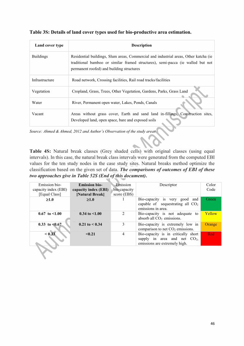
higher spatial resolution images in order to identify detailed land use types. Vegetation, water

bodies, vacant land, buildings, and other infrastructure (e.g. the transport network) were land

use classes utilized to determine bio-capacity. Details of these land use classes can be found in

Table 3S in the supplementary document.

A sufficient number of training samples that are representative of the area under

analysis are critical for accurate image classification using ERDAS Imagine software as used

in the present study. Training sites within the image are required to calibrate the software to

accurately identify each land cover type found within a given image being analyzed (Campbell

and Wynne, 2011). The sites used for the training samples were chosen based on reference data

and ancillary information collected from secondary sources; in this case Detailed Area Plans

for Dhaka, 2010 maps, and Dhaka City Corporation (DCC) Ward maps. After training sites

development, signature creation, and running maximum-likelihood classification algorithms in

ERDAS Imagine, five classified land cover types in the AOI’s were identified. These five land

cover types were merged into three broader types for the purpose of analyzing bio-capacity

they comprised: built-up areas, vegetation, and water bodies. In turn areas in the images

identified as one of these three types were assessed for classification accuracy. In the present

study, this accuracy assessment was conducted by a ground truthing cross check process. For

each land use class, GPS readings at five points were taken during field visits at each AOI.

Therefore, a total fifty points were available for the ten study areas (Table 45S, supplementary

document), with known land use for each point and these were then geo-referenced as point

features in GIS. Finally, from the error matrix, producers’ accuracy, user accuracy and overall

accuracy was estimated (Labib and Harris, 2018). The classified images were then utilized to

find the total area of each land cover type within each study area. These total areas were then

inputted into the bio-capacity estimation equation (eq4) and the bio-capacity of each study area

was determined.

2.6 Emission and bio-capacity index estimation

After completing the calculation of the amount of carbon uptake land that would be

required to completely neutralize a given study area’s CO2 emissions versus the bio-capacity

in global hectares (gha) for each of the ten AOIs an “Emission and bio-capacity index” value

was calculated for each AOI. The calculation of the index value is shown in eq5.

EBI = BC

C (eq5)

Where,

14

EBI = Emission bio-capacity index (EBI)

BC = Total bio-capacity of an area (gha)

C =Carbon Uptake land of that particular area (gha)

The emission bio-capacity index value represents the over or undershoot between the

value of carbon uptake land equivalent to 100% sequestration of GHG emissions and the

actually measured bio-capacity. Thus, EBI values of 1 imply that the bio-capacity is adequate

to sequestrate observed CO2 emissions produced from vehicle operations within the AOIs. EBI

values of 1 indicate that bio-capacity or bio-productivity are not great enough for full CO2

sequestration and or not producing enough bio-products of a value to offset the CO2 impact of

traffic related CO2 emissions. It should be noted that, Carbon uptake land have only been

estimated for traffic related CO2 emissions, other CO2 emissions such as industries, household

waste not been considered. Therefore, EBI values in this case only represent the traffic CO2

emissions situation and related bio-capacities. If other emission sources (e.g. Industries) been

considered, the overall EBI values may have changed, and then comprehensive bio-capacity

and emission scenarios might be identified, which is beyond the scope of this study.

For current study, EBI values less than 1 are categorized into three classes. These

classes are generated using the equal class interval method. Based on these classes, index values

are translated into an easy to understand single digit, whole number emission bio-capacity score

(EBS) value (1 to 4) and equivalent color code (e.g. red, orange, yellow, and green), in which

the value one which correlates with red represents very high net CO2 emissions and

correspondingly low bio-capacity as illustrated in Table 2. As presented in table 2, the EBI

value ranges and corresponding scores have descriptors to that convert the number values into

easily interpretable descriptions for wider audiences. The researchers chose the equal class

interval method as other approaches to classification such as the natural breaks method. Despite

natural break method provide better fit for the studied AOIs by optimizing the classes based on

EBI values, however this classification approach do not let standardization of this method for

other study areas, such as other cities. Nonetheless, the details of utilizing the natural breaks

method of classification can be found in Table 4S in the Supplementary document.

[Table 2 Near Here]

15

3. Results

3.1 Vehicular CO2 emission scenario in study areas

Bio-productive areas in the AOI’s was generally fixed or in decline (Ahmed and

Ahmend, 2012). Thus, the significant variable governing changes in net CO2 emissions and

the EBI index value was derived from vehicular exhaust. In turn, the composition of such

exhaust was dependent upon three sub-variables: vehicle type, fuel use and activity levels. The

results for these major sub-variables are discussed for each AOI in the following sections.

3.1.1 Vehicle type composition

Volume survey data represents the vehicle composition in the AOI under study. Fig 3

depicts the vehicle type composition in different study areas. Fig 3 shows that in most areas

automobiles generated the highest share of traffic volume. It also indicated that the highest

automobile usage was observed in areas V, VI and VIII (namely Gulshan 1, Science lab and

the Farm-gate area). By contrast, the greatest concentration of bus traffic was observed in areas

I, VII, X, IX (namely Mirpur 10, Mog-bazaar, Jatrabari and Motijheel area). CNG auto-

rickshaw and motorcycle were a moderately dominant mode of travel in all study areas. Other

modes (jeep, pick-up, leguna, and taxi) comprised an insignificant share of overall traffic

composition.

[Fig 3 Near Here]

3.1.2 Vehicle classes aggregate share of CO2 emissions and per-capita emissions

Each vehicle class has different emission characteristics and emission factors based on

its engine type and power, age of engine, type of fuel consumed, fuel efficiency etc. Fig 4

shows variations in CO2 emissions from different vehicle types in all AOIs. It is clear that

except Area V the highest levels of CO2 emissions observed were derived from bus service,

followed by automobiles. CNG fueled buses were found to have the highest per vehicle

emission factor (968 gm/km) among all the types of vehicles observed. For example, the

emission factor for CNG fueled automobiles was less than one-third (237 gm/km) as much as

that for CNG fueled buses. Despite automobiles comprising the majority of traffic, due to their

lower emission factors they contributed less CO2 emission compared to buses on a per vehicle

basis. Overall, however, Fig 4 makes clear that automobiles and buses generated between 60

and 70% of all CO2 emissions in the AOIs.

[Fig 4 Near Here]

16

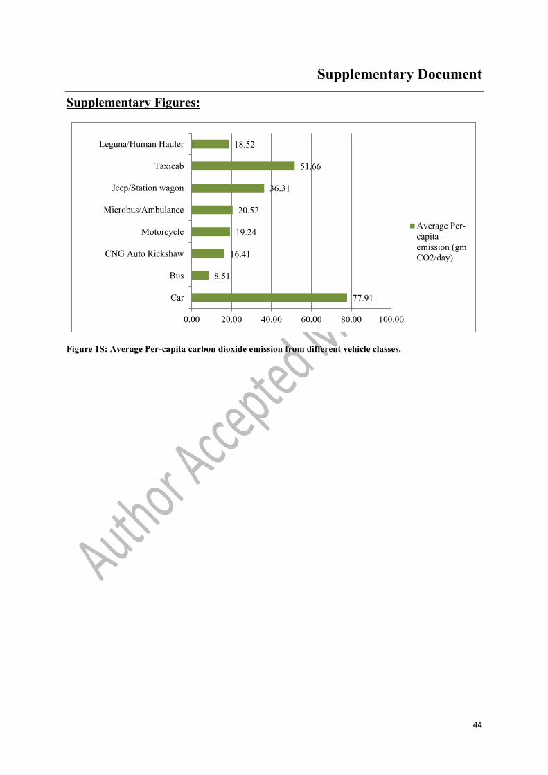
Emissions per vehicle is an insufficient measure of CO2 emissions versus person-miles

traveled in urban traffic. What is key to understanding traffic volume versus emissions

observed is to examine the value for the per-capita emissions for different vehicle classes in

the AOIs. For example a full bus may have a much lower per-capita emissions value than other

classes of vehicles in traffic despite having the largest per vehicle emissions value. Per-capita

emissions for each vehicle class (Figure 1S, supplementary document), have been estimated

using vehicle occupancy data obtained from Labib et al., (2014). Analysis of estimates of per-

capita vehicle usage show that emissions per passenger are highest from automobiles. By

contrast, public transit buses have the lowest per-capita emissions. Aggregating all the AOIs

studied, the per-capita emissions generated by automobiles were ten times higher than the per

capita value for buses. This result is consistent with other studies such as Wang et al. (2017)

and Wang et al. (2015), whose reported results were similar to those in the present study, with

buses having the highest occupancy and thus the lowest per-capita CO2 emission levels.

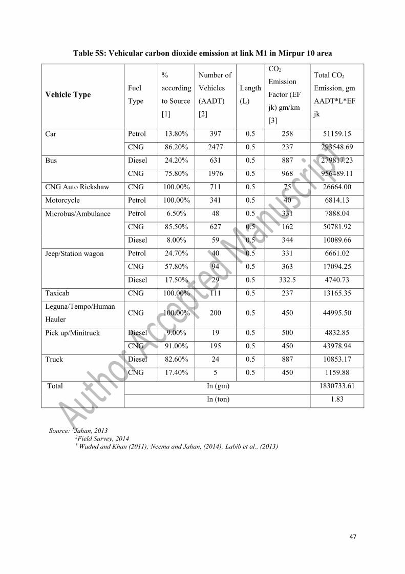
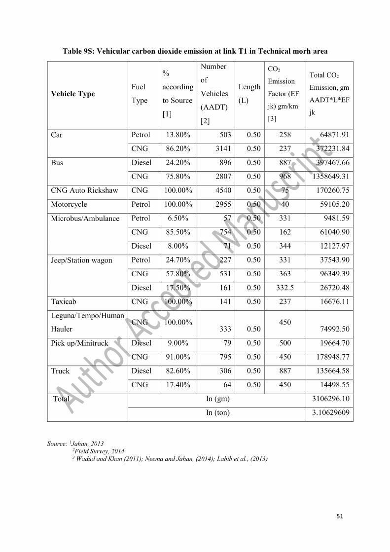
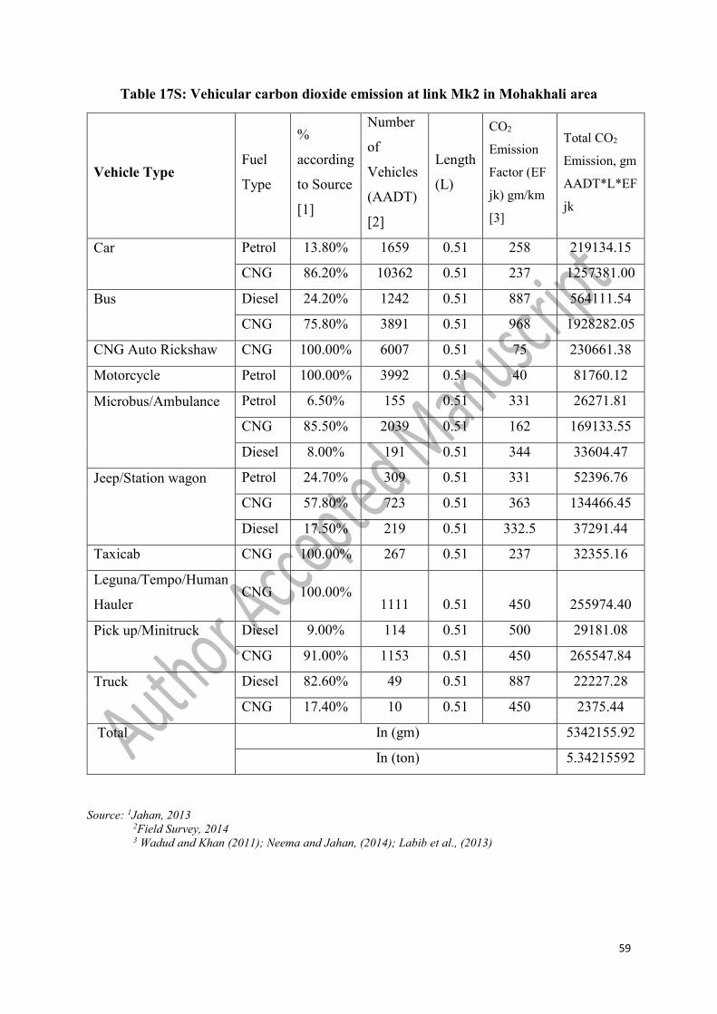
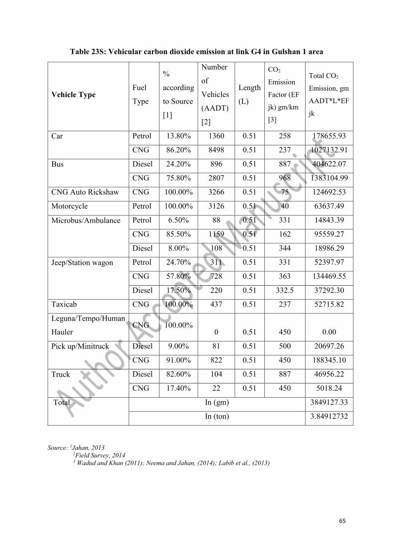
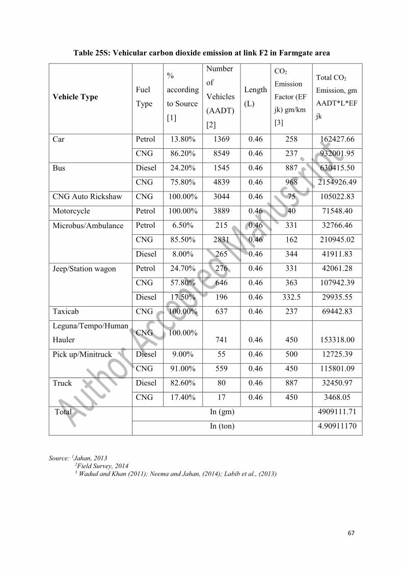
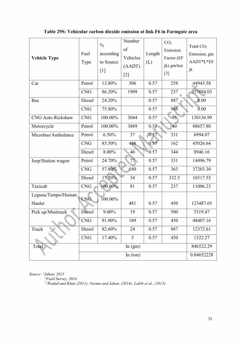
3.1.4 Total CO2 emissions in each AOI

This section provides estimates of total CO2 emissions from the transportation sector

for the studied AOIs. In order to determine the total daily CO2 emissions from each AOI,

emissions data for traffic on all links within each study area were combined. Annual emissions

were projected by multiplying the number of days in a non-leap year by the net CO2 emissions

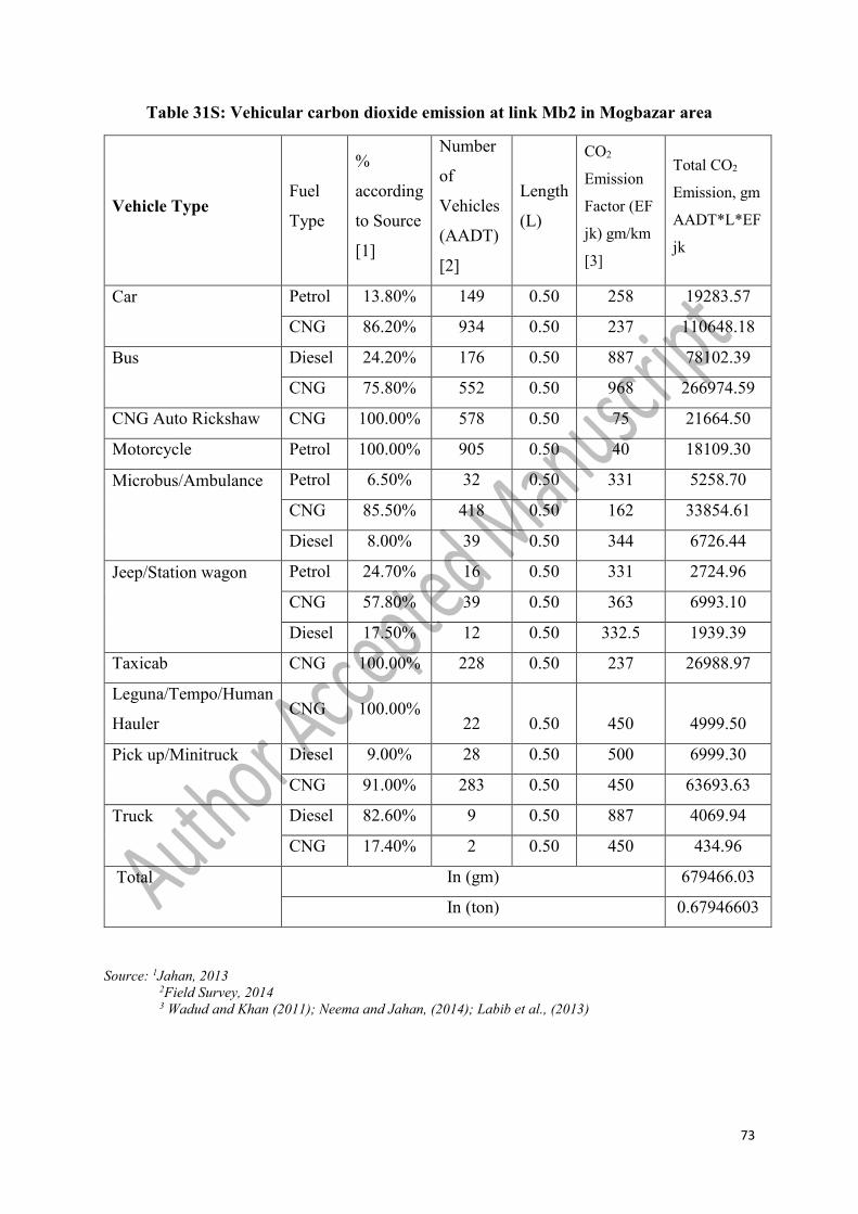
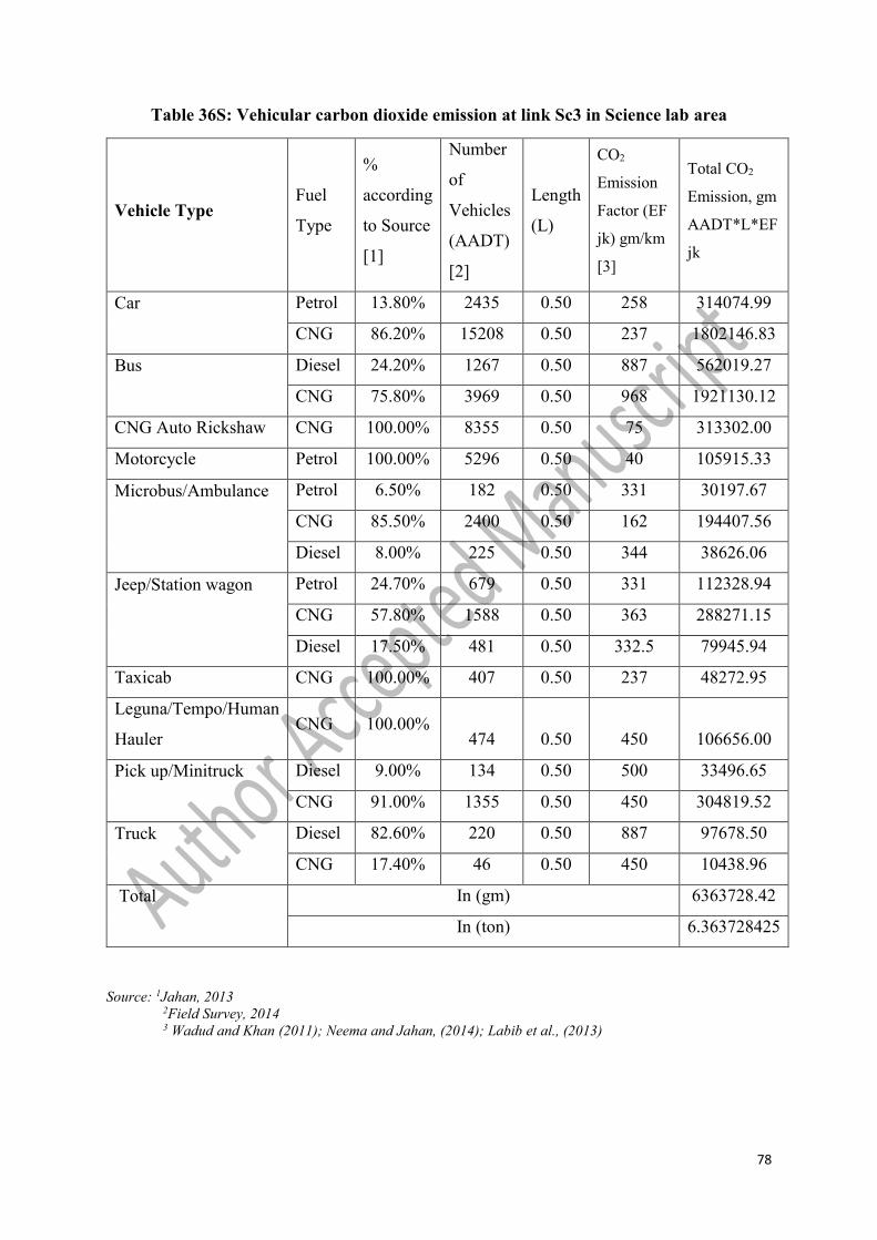
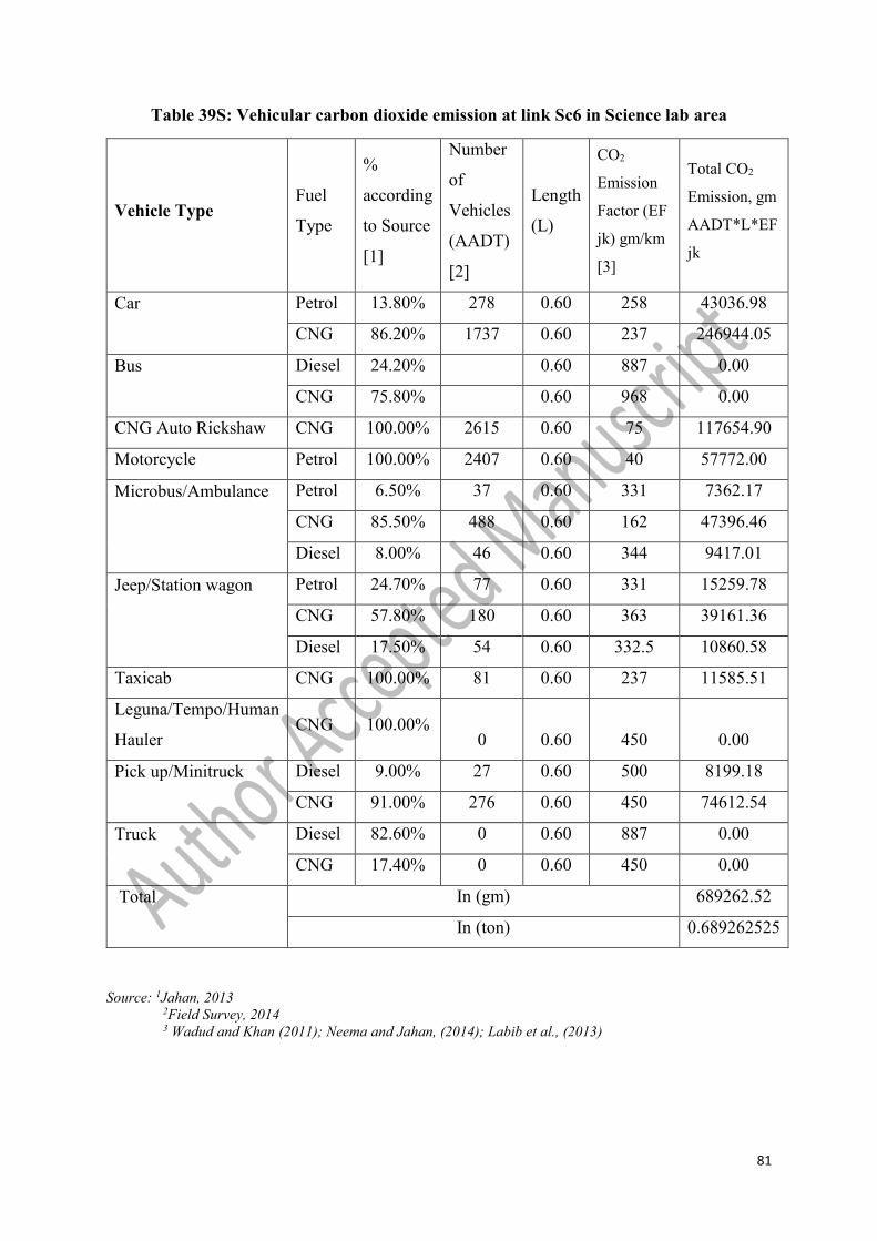
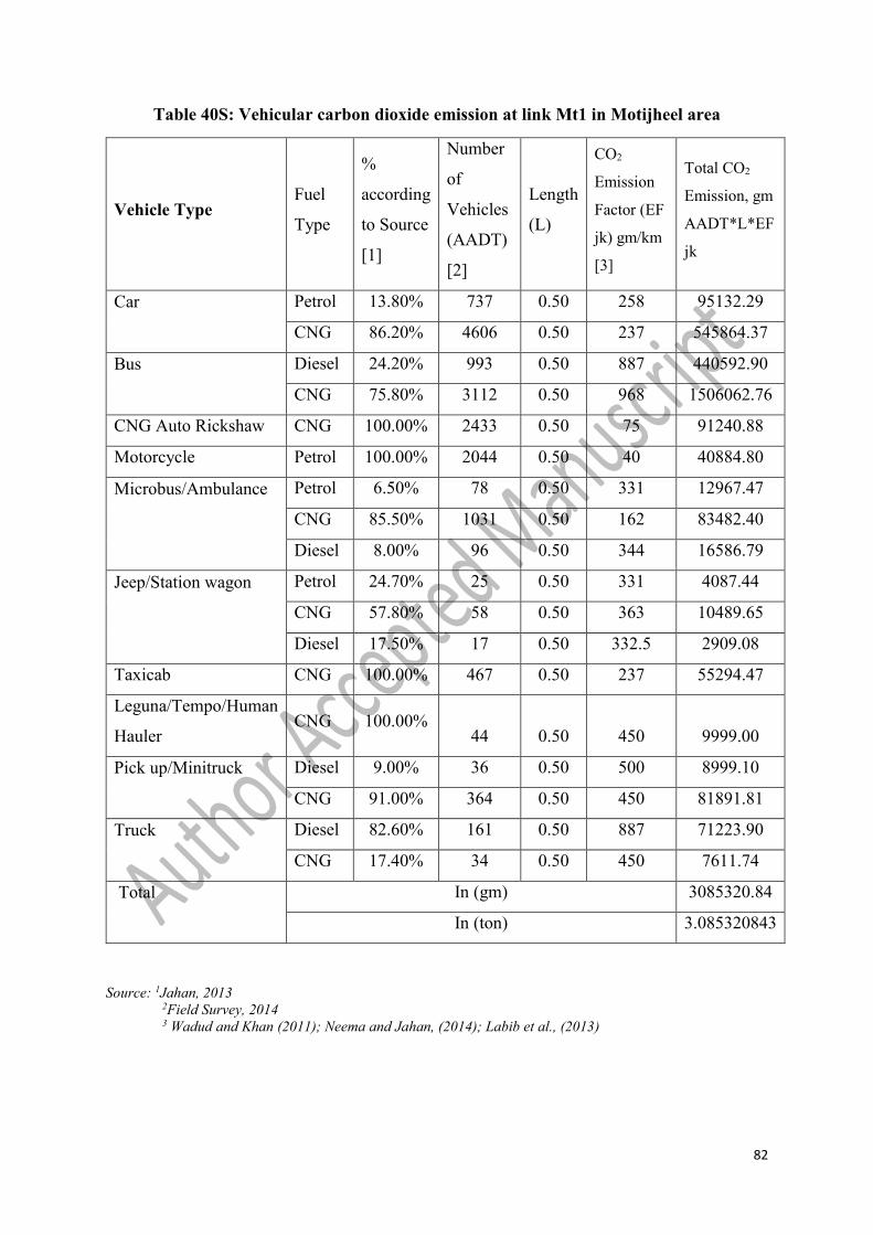
calculated for each AOI daily, as shown in Table 3. Details of daily and yearly CO2 emission

for all AOIs can be found in Table 47S, in the supplementary document. As illustrated in table

3 ‘Total tons of CO2 in a year’ column, the lowest CO2 emissions occurred in Area I; by contrast

the highest CO2 emissions were observed in Area X the most active node in the city

transportation network. Higher CO2 emissions levels correlated with higher levels of

transportation activities in the AOI’s in the present study. This was not only illustrated by very

high levels of traffic in Area X but also by the low levels of traffic in Area I. Detailed Area

Plan land use data supported this as well as our findings that Area I was predominantly

residential and thus supporting fewer commercial and administrative activities (Labib et al.,

2014). As a result, Area I generated less transportation activity and hence fewer emissions. Its

predominantly residential nature also meant that it was an area of trip production, rather than

trip attraction. Combining all AOIs in the present study generated an average value for CO2

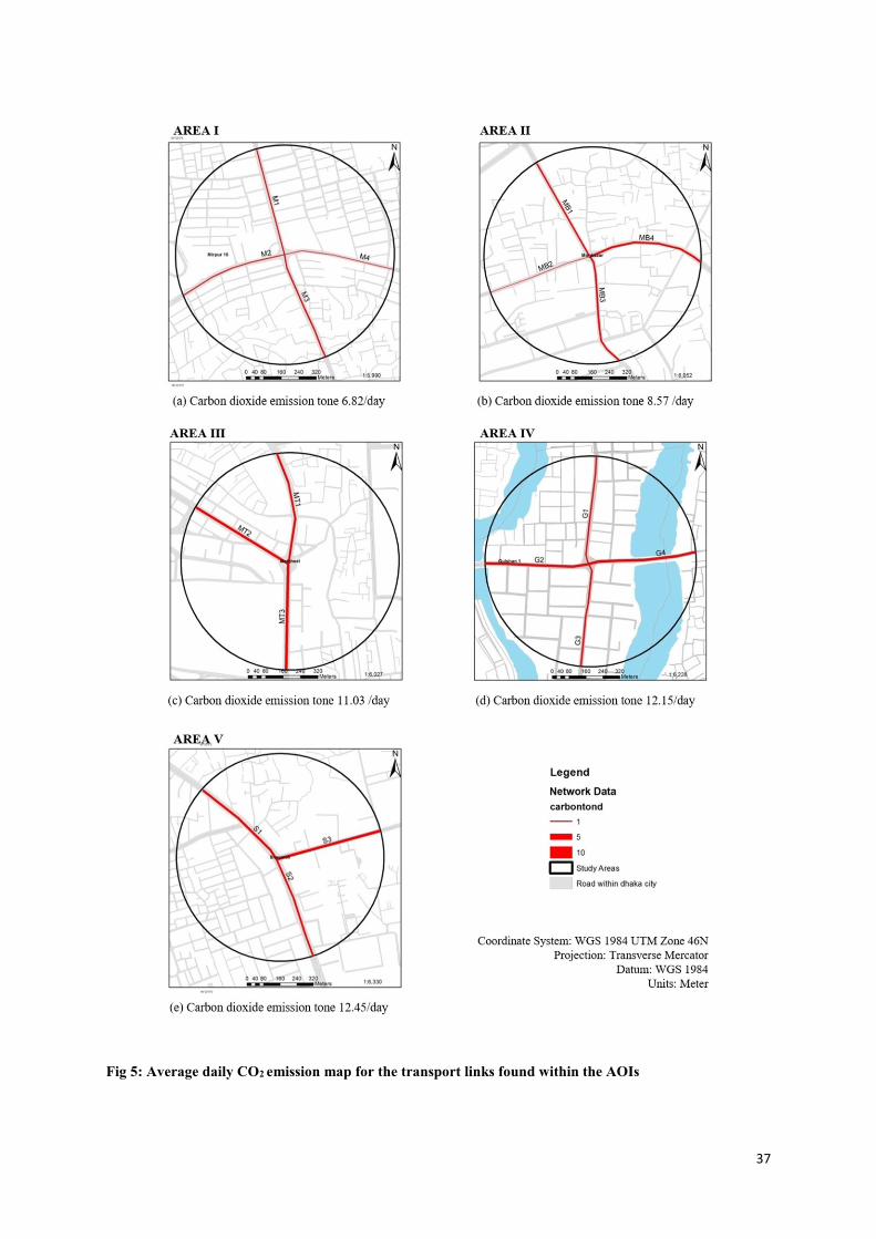
emissions of thirteen tons of CO2 emitted per day. Fig. 5 and Fig 6 show the quantity of CO2

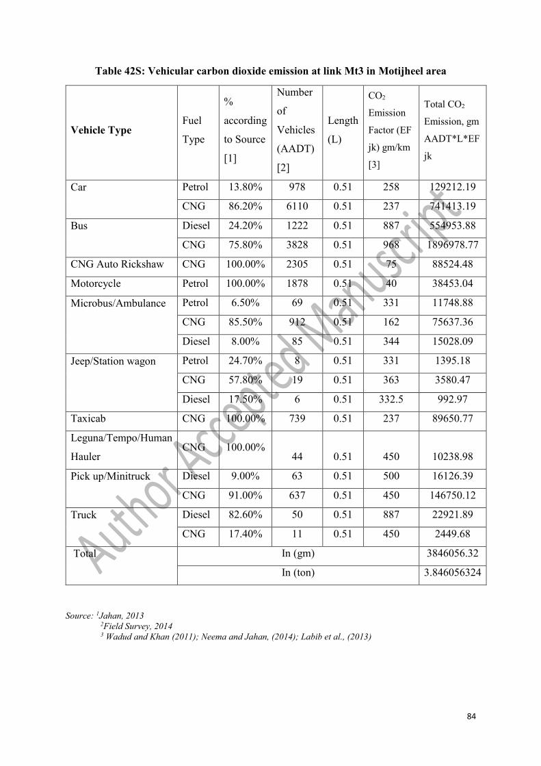
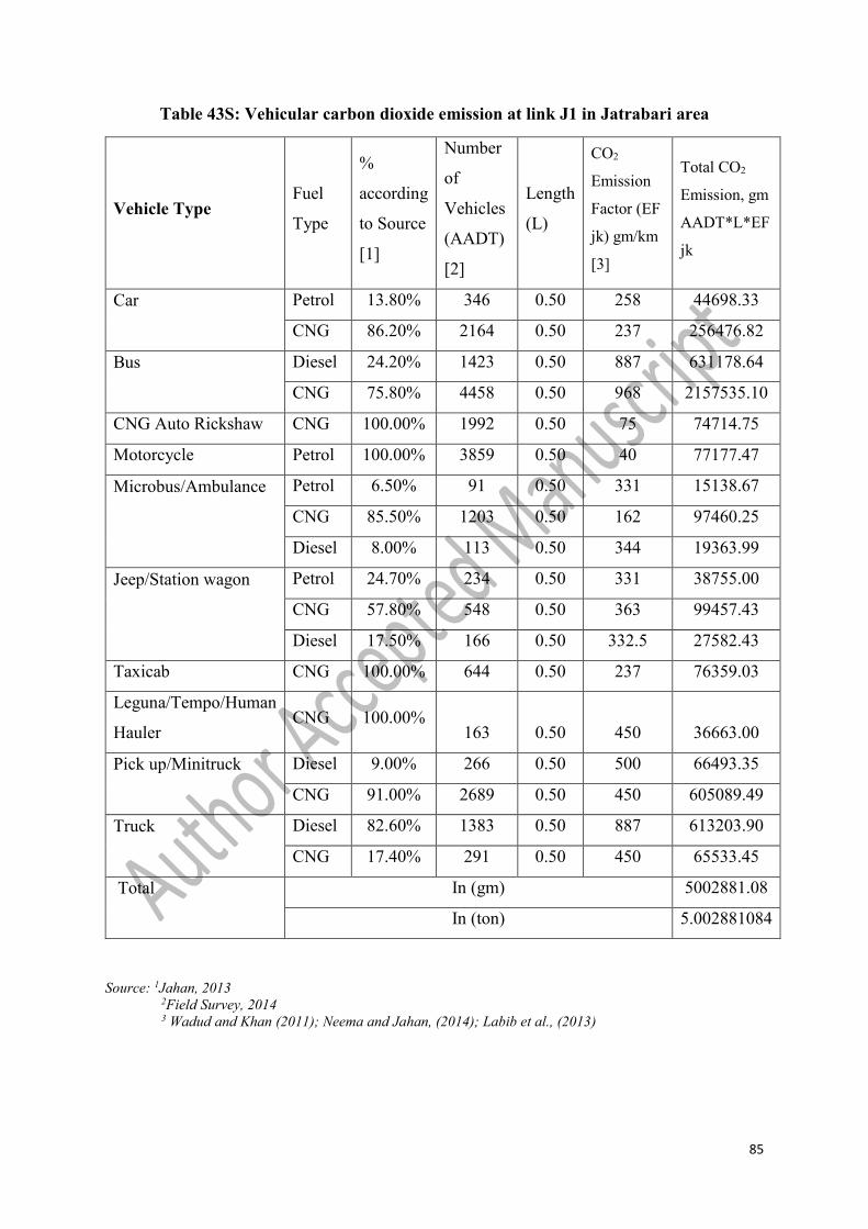
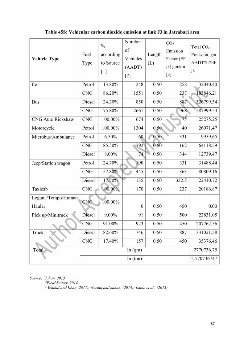
emissions mapped to the AOI’s in the present study. The emissions calculation for each link

within each AOI is presented in Table 5S-46S, Supplementary Document.

17

[Figure 5 Near Here]

[Figure 6 Near Here]

3.2 Carbon Uptake Land equivalent to CO2 emissions in AOIs

Utilizing the estimated CO2 emissions from transportation activities in each AOI, the

carbon uptake land value that would be required to absorb all CO2 emissions in each AOI was

determined. Table 3 presents a summary of the estimated amount of carbon uptake land that

would be required to neutralize and sequester all CO2 emissions at the time of the present study.

The table shows that the largest carbon uptake land value would be required for areas IV and

VIII (Farm-gate and Science Lab). By contrast the lowest carbon footprint was found in areas

I and VII (Mirpur 10 and Mog-bazaar). For all cases, the carbon uptake land value required

was calculated by multiplying total net annual CO2 production with the appropriate conversion

factors, first for sequestration of all CO2 emitted expressed in tons per acre per year, followed

by a conversion of this value to hectares and finally a conversion of the hectare value to global

hectares to arrive at the estimated carbon uptake land area expressed in global hectares. These

estimated carbon uptake land (C) values were then utilized as input values to eq5 in determining

the EBI values.

[Table 3 Near Here]

3.3 Bio-capacity of each AOI

Bio-capacity is one of the major constituents of the EBI. Therefore, the value for the

biological capacity of each AOI was estimated utilizing eq4 in the methodology section. The

outcomes of the bio-capacity estimation process are described below.

3.3.1 Bio-productive areas

For bio-capacity estimation three broad categories of land use types were identified

namely: i) built-up areas (comprising buildings, infrastructure, roads), ii) vegetation, and iii)

bodies of water. Figures 7 and 8 represent the results of the present study’s land surface

classifications in each AOI. It is evident that, among the three classes, built-up land represented

most of the hectarage in each AOI with the exception of areas V (Gulshan 1) (Figure 7d) and

II (Technical Morh) (Figure 8f). Nine of the AOIs had limited areas of open water and area VI

(Farm-gate) within the selected buffer range (Fig. 8j) had no open water area whatsoever. The

greatest quantities of vegetation were found in areas II (Technical morh) as shown in Fig. 8 (f)

and I (Mirpur 10) as shown in Fig. 7 (a). The lowest quantity of vegetation was found in area

18

X (Jatrabari area) as presented in Fig. 8 (g). The hectarage values calculated for each of the

three classes of land use types were utilized to determine the actual bio-capacity of the AOIs.

[Fig 7 Near Here]

[Fig 8 Near Here]

Employing an error matrix accuracy test on the classified images was required to check

the accuracy of the classification process. Correlating the error matrix producer’s accuracy and

the user’s accuracy provided a determination of overall accuracy (Table 49S, Supplementary

Document). The Kappa coefficient was also verified. Producers’ and users’ accuracies were

found to be over 80% for the built-up and vegetation classes. Overall accuracy of image

classification was 84% and the kappa coefficient value was 0.75 (Table 50S, Supplementary

Document). Kappa values. Generally a kappa value of more than 0.80 indicates that image

classification was both very good and highly acceptable, however values of more than 0.75 are

widely acceptable (Lillesand et al., 2014; Campbell & Wynne, 2011). Accuracy Test points,

with GPS coordinate values for UTM zone 46 N for the AOIs are presented in Table 48S in

Supplementary Document.

3.3.2 Bio-capacity of selected areas

Utilizing the land use areas identified from the analyzed images and eq4, the bio-

capacity (BC) value for each AOI was determined. As an example, Table 4 illustrates the

calculation process utilized to calculate the bio-capacity for Area I (Mirpur 10). It was found

that the total bio-capacity was approximately 267.8 gha. Employing this calculation

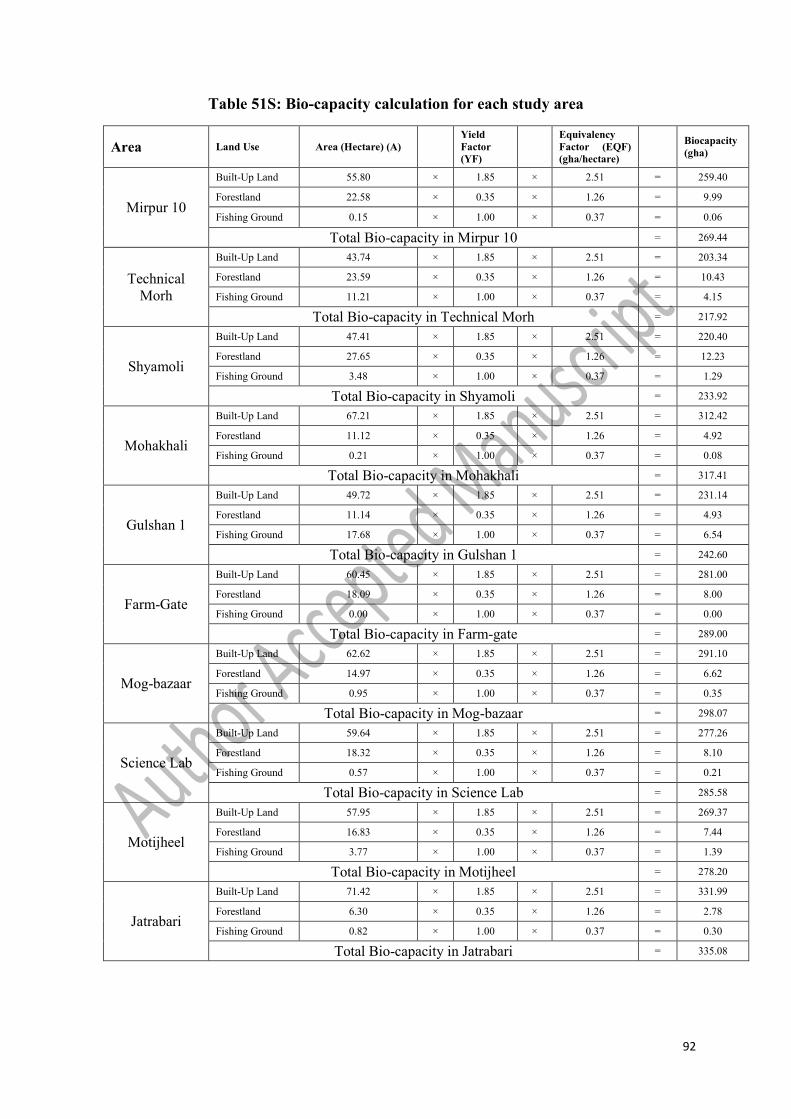
methodology the bio-capacity for each AOI was determined. The results for each AOI are

summarized in Table 5 under the ‘Bio-capacity Area’ column. The actual bio-capacity

estimation calculations for each AOI are provided in Table 51S in the supplementary

document.

[Table 4 Near Here]

Table 4 illustrates that, the yield factors for built-up areas are greater than those for

forest or bodies of water, hence the estimated bio-capacities of built-up areas have higher

values than those for vegetation and water bodies. This apparently counter-intuitive result can

cause confusion for readers not familiar with the theory supporting the concept of National

Footprint Accounts (NFA) and bio-capacities. According to the NFA bio-capacity is defined

19

as “the biosphere’s supply (bio-capacity) of ecosystem products and services in terms of the

amount of bio-productive land and sea area needed to supply these products and services.”

(Boruke et al., 2013, p 518). However, due to lack of data unavailability regarding the bio-

productivity of built-up areas, built-up land is considered the equivalent of cropland in terms

of world average productivity (Galli, 2015; Borucke et al., 2013). This assumption is

developed on the basis of the observation that, in general human settlements (e.g. Urban areas,

built infrastructure) are located in fertile areas which may had the potentials for high yielding

cropland (Borucke et al., 2013; Wackernagel et al., 2002). As a result of this assumption,

despite having no photosynthesis and thus no direct bio-productivity from built-up land,

considering yield factor of cropland as yield factor for built-up areas over or underestimates

total bio-capacity.

In this case, as cropland in Bangladesh has a higher yield factor than either forest or

bodies of water (Table S1, Supplementary document), and cropland is used as a value

equivalent for built-up areas, the consequence is that built-up areas have a higher yield factor

than forest’s or bodies of water. Nonetheless, this equivalence allows to create a dummy-value

for the productivity that occurs in these areas. It should be noted that, due to inherent theoretical

limitation of NAF’s bio-capacity estimation process, current study may over/under estimated

the bio-productivity of built-up areas compared to vegetation and waterbodies. In reality to

improve overall bio-capacity, more vegetation cover and water bodies with greater yields

would act as positive contributors, in contrast increasing built-up areas would only reduce

overall bio-capacity.

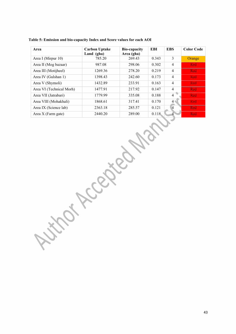
3.4 Emission and bio-capacity index values

Dividing the bio-capacity (BC) area by the estimated carbon uptake land value (C)

allows the EBI to be determined. Table 5 shows that nine out of ten areas possess EBI value

of 0.33 which equates to a EBS of 4, both of these values imply that bio-capacity is in critically

short supply in these areas and net CO2, emissions are extremely high. With the exception of

Area I (Mirpur 10) all other AOIs would require the addition of very large amounts of bio-

productive land within their geographical boundaries if they were to have the capacity to absorb

all the net CO2 emissions currently emitted by the transportation sector in each respective AOI.

The very high amounts of net CO2 emissions are strongly related to high and continuously

increasing traffic volumes and high usage levels for private vehicles but may also suggest that

there are inefficiencies inherent in operating old or poorly maintained vehicles, related to

poorly tuned engines, nonfunctioning or ineffective pollution controls on engines and related

20

issues pertaining to excessive use of fuel. Overall, Table 5 conclusively demonstrates that the

amount of bio-productive area within the AOI’s is inadequate to sequester all emitted CO2, and

illustrates the serious gap between levels of CO2 production and CO2 sequestration.

[Table 5 Near Here]

Both the raw data-take and the calculated EBI values are highly indicative of the very

high levels of CO2 emissions from transportation activities in nine of the ten AOIs. It clearly

indicates that the overall emissions of CO2 from the transportation sector in Dhaka are well in

excess of levels that available bio-capacity can remediate or counter balance. Indeed, the

carbon uptake land value that equates to the ability to sequester all CO2 emissions from the

transportation sector in Dhaka is a hectare value larger than the hectare value for all land within

the city limits (Labib et al. 2013).

4. Discussions

4.1 Major Factors Contributing to higher CO2 emissions and lower EBI values

The present study’s analysis highlighted several factors responsible for the high net

CO2 emissions in Dhaka. Results showed that both the composition of vehicular traffic and

the limited bio-capacity of extant land cover types contributed to observed high net emissions.

Those AOIs with lower EBI values closely correlated with higher levels of vehicular activity

and more built-up land use area within the AOI. In these areas, the volume of daily vehicular

traffic through the links of each AOI was quite large. These AOIs were exemplified by high

traffic volume, host intersections characterized by intermittent spikes in volume, and

differentiation between trip originating and terminating traffic. Traffic nodes in AOIs such as

Farmgate (Area X) and Science Lab (Area IX) explicitly exhibit these characteristics.

Therefore, it can be implied that, intermittent nodes (usually having higher connectivity) which

connect more trips need careful design, and more effective traffic regulations to assist in

controlling CO2 emissions, as higher traffic density would likely raise levels of such emissions

(Ferreira and d'Orey, 2012).

The results of the present study also indicate that lower EBI value (and corresponding

high EBS score) traffic network nodes are characterized by high levels of private vehicle usage

(e.g. automobiles and motor bikes) versus the use levels of public transit such as buses. This

finding is common to a number of recent studies including Iqbal et al, (2016), Kamruzzaman

et al., (2015); and Druckman and Jackson, (2008). Equally, it is clear from the present study’s

results combined with that increases in motorized traffic both public and private are the driving

21

force for increases in overall net CO2 emissions from the transportation sector in Dhaka (Labib

et al., 2013). As Bangladesh continues to experience a growing economy, the affordability of

private vehicles increases in lock-step among private citizens (Islam et al., 2016). Furthermore,

until now there has been no effort made to control the usage of private vehicles in Dhaka, and

no restrictions for private vehicles on busy and crucial nodes. Thus, a large and increasing

component of the increase in motorized traffic comprises of personal vehicles which are

becoming a major component in future increases in CO2 emissions in Dhaka from

transportation.

Another factor contributing to CO2 emissions in Dhaka is an obsolescent traffic signal

system. In Dhaka no coordinated system of traffic signals geared to optimizing traffic patterns

and traffic throughput exists. The current signal system was not designed for either current or

projected levels of traffic. Indeed, the current signal system has such limited capacity that in

the AOIs researchers observed traffic police manually attempting to coordinate traffic signals

during periods of high traffic volume, for example Farmgate (Area X) experiences massive

traffic congestion the majority of each day. This congestion is abetted by the fact that the signal

systems on different links in the area are not coordinated with each other. As a result, traffic

police are required to assist in controlling traffic. However, they must use their personal

judgment, uninformed by conditions at other intersections, as to how much time ought to be

allocated to each phase of the signal cycle in order to optimize overall traffic flow in all links

in the intersection they are attempting to control. These inadequacies of the present system

observed during the present study appear to actually contribute to inducing massive congestion

on some links in the AOIs. Unfortunately, such congestion is associated with increased trip

times, increased costs to human health and much increased CO2 emissions (Iqbal et al., 2016;

Labib et al., 2013). Ferreira and d'Orey, (2012) demonstrated that, a well-organized intelligent

transportation system (ITS) based traffic signaling system is effective in mitigating CO2

emissions in high density traffic areas.

The major arterial roads of Dhaka do not provide access for fuel free transport modes

such as bicycles or rickshaws (Mahmud et al., 2012). In this study, the nodes examined in the

AOIs were connecting major arterial roads, It must be noted that FFTs do not emit CO2, and

they are widely used in secondary or access roads in Dhaka city (Labib et al., 2016). However,

while it might be speculated that the absence of FFTs on major roads might be a reason for

greater CO2 production in these nodes due to the increased use of motorized alternatives there

is the issue highlighted by the present study that major arteries in Dhaka are near, at, or over

22

their capacity limits. Injecting slow-moving FFTs with limited passenger carrying capacity

into arterial traffic could actually lower overall passenger throughput on these arteries and

increase emissions due to further increasing congestion caused by mixing FFTs with motorized

traffic on major arteries. Furthermore, mixing FFT’s and motorized transport on major

roadways causes serious safety issues and is a practice discouraged world-wide in urban

settings. However, given the popularity of FFT’s in Dhaka and their environmentally benign

nature it is possible that exploring the possibility of providing dedicated lanes for FFTs might

provide the path to an effective solution.

Another major problem existing in Dhaka’s traffic is related to the abundance of unfit

vehicles on the road. During the traffic volume survey the researcher observed a predominance

of older vehicles often exhibiting major deficiencies in maintenance, both public (e.g. bus) and

private (e.g. jeep, station wagon) in traffic. Field observation showed, that often these vehicles

had been marked by the traffic police as unfit. Upon inquiry as to why so many such vehicles

were to be seen in traffic it became apparent that irregular inducements provided by the owners

of the vehicles to avoid formal legal action were common. Thus, weaknesses both in the

practice of policing and in the justice system are transport issues insofar as they contribute to

allowing both unsafe and high emitting vehicles to remain on the road in Dhaka.

A final issue is the levels of vegetation growing in the AOIs. Neema and Jahan (2014),

found that the presence of increased amounts of road side vegetation correlates with higher

levels of CO2 sequestration along such roadsides. However, the AOIs in the present study had

little greenery growing directly along their links or, indeed, anywhere within their overall areas.

4.2 Impacts and way forward

From an ecological point of view, the transportation system in Dhaka is not sustainable

due to the fact that its extant bio-productive areas cannot sequester even a large fraction of

current CO2 emission levels. Furthermore, the areas of the city devoted to land uses that

support what bio-capacity exists are shrinking (Hassan and Southworth, 2017). Further

shrinkage of bio-capacity in a city whose population and hence, traffic levels continue to

increase suggest that net CO2 emissions both from traffic activities and other activities will also

continue to increase. Such increases will, in turn intensify heat-island effects as well as

supporting increases in other air pollutants besides CO2 (Harlan and Ruddell, 2011; Han and

Naeher, 2006).

23

4.2.1 Policy Implications

The rating system created for the present study may aid in both planning professionals

and policy makers being able to more easily grasp the severity of the CO2 emissions problem

under current and projected conditions. The index may also act as a surrogate value for the

negative impact emissions have on health, livability and the environment in Dhaka. Based on

the results of the current, several policy initiatives recommended to improve the overall

sustainability, livability and environment of Dhaka.

Public Transit

The Strategic Transport Plan 2005 for Dhaka recommended introducing bus rapid

transit (BRT) in the main corridors of the city as an effective and efficient solution to resolve

the poor service quality and capacity constraints of current bus systems in Dhaka. Despite

having been recommended as long ago as 2005 this is an excellent suggestion with even greater

merit, due to urban growth, than when it was first mooted (Rahman et al., 2012). Additionally,

as of 2017 the authors note that a new Mass Rapid Transit is under construction in Dhaka in

association with JICA, and this may change the composition of traffic in Dhaka with a greater

emphasis on public transit. However, experience in other major cities particularly in

developing economies suggests that as long as the numbers of private vehicles continues to

increase; a highly likely scenario in a country with a growing economy and a growing middle-

class, any reduction in overall CO2 emissions and congestion on surface routes will likely be a

transitory one.

Low Emissions Zones

Apart from attempts to engender a travel demand shift by promoting public transit (e.g.

Metro, BRT), FFTs, and encouraging mixed land use (McBain et al., 2017; Nakamura and

Hayashi, 2013) in Dhaka, low-emission zone initiatives could be an effective solution to calm

traffic intensities and CO2 production in key nodes (or highly connective nodes). For example,

nodes in AOIs VIII, IX, and X might have low emission zoning strategies implemented to

discourage the number of trips with private vehicles. Despite having potential political

difficulties in implementation, low emission zoning policy could be implemented with

relatively little cost and within a short period of time. Implementation of low emission zones

appears a reasonable solution, similar to the low emission zones in London (Ellison et al., 2013)

and other European cities (Dias et al., 2016; Holman et al., 2015).

24

Improved Traffic Management

Another policy intervention might be needed in improving the traffic management

system. A key component to minimizing both emissions and maximizing quality of life is the

design of a modern traffic management plan for Dhaka supported by a high-capacity and fully

functional traffic signaling system optimized to maximize traffic throughput. The authors

strongly recommend replacing the current obsolete system requiring continuous human

intervention by traffic police with a new optimized signaling system using ITS (Satyanarayana

et al., 2018). Gains in economic efficiency and productivity within Dhaka may well yield more

than the cost of such a system.

4.2.2 Other potential low-carbon interventions

In addition to a traffic calming strategy, a ride-share program may be an effective

solution in the context of Dhaka’s needs. Labib et al., (2013) suggested that, carpool or car

share initiatives might be effective in Dhaka and as of 2016 such services have been

implemented in the city in with relatively limited coverage. Additionally, private rideshare

services such Uber and Pathao-Moving Bangladesh (a local ride-sharing company providing

motor-cycle rides), both introduced in 2017, have been gaining popularity among those needing

transportation in Dhaka. At least two recent studies had results suggesting that ride-share

services have successfully reduced private/personal vehicle usage and congestion in urban

areas in which such services were introduced (Li et al., 2017; Alexander and González, 2015).

Thus, officially encouraging and monitoring ride-share services may to some extent, assist in

ameliorating traffic induced CO2 emissions.

Urban greening initiatives including road side tree plantation, green roof creation, green

wall installation and other green infrastructure creation would not only assist in CO2

sequestration but also in overall improvements in living conditions, quality of life and even

storm water control. In particular among the studied AOIs due to their extremely low EBI

values, Area V, VI, IX, and X would appear to require immediate action to improve their

vegetative coverage utilizing some rapid measure such as Green roofs and green walls (Rowe,

2011).

5. Conclusion and further development

With the growing concern for CO2 emissions resulting from vehicular traffic it has

become necessary to better understand and identify the areas within cities such as Dhaka where

CO2 emissions from vehicles have outstripped the local capacity to absorb and sequester such

25

emissions along with associated emissions that can be a direct threat to human health. In light

of this need the present study has as one of its key purposes the development of an EBI rating

system that would assist in identifying the traffic routes and zones within an urban

transportation network that are deemed ecologically unsustainable due to high net CO2

emissions and low local bio-capacity. This rating system combines the domain of traffic

emission related studies with ecological footprint and bio-capacity related studies. In turn this

has allowed the establishment of index values for the previously missing relationship between

urban transportation systems and their local environments.

The present study utilizing the EBI successfully mapped and measured net CO2

emissions at key traffic nodes in Dhaka. As a result, it provided an understanding of the CO2

sequestration capacity associated with each AOI but more importantly it created a map

overlaying the traffic network highlighting problem areas using an index that is easy to grasp

for policy makers. The EBI rating system found very high (level 4, code red) index values

correlated with very low CO2 absorption and high net CO2 emissions at nine out of ten key

nodes. Thus of the ten nodes only one was moderately sustainable as defined by having the

capacity to absorb a considerable amount of the CO2 emissions in its local area. Based on the

results, it is reasonable to conclude that the nodes with lowest EBI values require urgent

attention to ameliorate both their current net CO2 emissions as well as control future increases

in such emissions.

While identifying critical nodes as ecologically unsustainable as they currently stand,

in the Dhaka road network was one proximate reason for conducting the present study a wider

goal was to create an index that reduces the many potential factors impacting net emissions to

a single digit number and associated colour. This, in turn, allows the creation of coloured map

overlays for urban areas highlighting problem areas clearly while also showing their

relationship to one another and to the underlying transportation networks at a glance. It is the

opinion of the authors that it is not enough to know the facts but necessary to be able to convey

them clearly and easily especially to policy makers and potentially to other interested groups

and/or the wider urban population. Finally, given sufficient data and adequate simulation

software the EBI could be valuable as one output modality for modeling different outcomes in

‘What-if’ scenarios of CO2 emissions, with the EBI value and color changing as parameters

such as: traffic intensity, signal optimization, different road surfaces and differing levels of

vegetation inter alia are varied.

26

Despite the careful attention of the authors, this study is not presented as being

comprehensive. It would benefit from further testing of the new index as well as potentially

improving on the measurement techniques used in the index creation process in order to further

refine the index to ensure the most robust results.

Conflict Of Interests

No potential conflict of interest was reported by the authors

Acknowledgement

We would like to thank Mr. Zahid Hasan Siddiquee of Institute of Water Modelling,

Bangladesh for his input regarding the collection of remote sensing data for the study area.

Thanks to Dr. Md. Musleh Uddin Hasan and Jinat Jahan of Department of Urban and Regional

Planning for their comments in conducting this study. We would also like to thank the

anonymous reviewers of this paper for their constructive comments and suggestions.

References

Afrin, T., Ali, M. A., Rahman, S. M., & Wadud, Z. (2012). Development of a Grid-Based Emission

Inventory and a Source-Receptor Model for Dhaka City. In Floria: The US EPA’s

International Emission Inventory Conference. Accessed April (Vol. 4, p. 2013).

Ahmed, B., & Ahmed, R. (2012). Modeling urban land cover growth dynamics using multi-temporal

satellite images: a case study of Dhaka, Bangladesh. ISPRS International Journal of Geo-

Information, 1(1), 3-31. DOI:10.3390/ijgi1010003

Alexander, L. P., & González, M. C. (2015). Assessing the impact of real-time ridesharing on urban

traffic using mobile phone data. Proc. UrbComp, 1-9.

Amekudzi, A. A., Khisty, C. J., & Khayesi, M. (2009). Using the sustainability footprint model to

assess development impacts of transportation systems. Transportation Research Part A: Policy

and Practice, 43(4), 339-348. DOI: https://doi.org/10.1016/j.tra.2008.11.002

27

Andrews, C. J. (2008). Greenhouse gas emissions along the rural-urban gradient. Journal of

Environmental Planning and Management, 51(6), 847-870. DOI:

https://doi.org/10.1080/09640560802423780

Borucke, M., Moore, D., Cranston, G., Gracey, K., Iha, K., Larson, J., Lazarus, E., Morales, J.C.,

Wackernagel, M. and Galli, A., (2013). Accounting for demand and supply of the biosphere's

regenerative capacity: The National Footprint Accounts’ underlying methodology and

framework. Ecological Indicators, 24, pp.518-533.

Campbell, J.B., & Wynne, R.H. (2011). Introduction to remote sensing. New York, NY: Guilford

Press.

Dewan, A. M., & Yamaguchi, Y. (2009). Land use and land cover change in Greater Dhaka,

Bangladesh: Using remote sensing to promote sustainable urbanization. Applied

Geography, 29(3), 390-401. DOI: https://doi.org/10.1016/j.apgeog.2008.12.005

Dias, D., Tchepel, O., & Antunes, A. P. (2016). Integrated modelling approach for the evaluation of

low emission zones. Journal of environmental management, 177, 253-263. DOI:

https://doi.org/10.1016/j.jenvman.2016.04.031

Dodman, D. (2009). Blaming cities for climate change? An analysis of urban greenhouse gas

emissions inventories. Environment and Urbanization, 21(1), 185-201. DOI:

10.1177/0956247809103016

Druckman, A., & Jackson, T. (2008). Household energy consumption in the UK: A highly

geographically and socio-economically disaggregated model. Energy Policy, 36(8), 3177-

3192. DOI: https://doi.org/10.1016/j.enpol.2008.03.021

Ellison, R. B., Greaves, S. P., & Hensher, D. A. (2013). Five years of London’s low emission zone:

Effects on vehicle fleet composition and air quality. Transportation Research Part D:

Transport and Environment, 23, 25-33. DOI: https://doi.org/10.1016/j.trd.2013.03.010

Ewing, B., Reed, A., Galli, A., Kitzes, J. and Wackernagel, M., 2010. Calculation methodology for

the national footprint accounts.

Fan, F., & Lei, Y. (2016). Decomposition analysis of energy-related carbon emissions from the

transportation sector in Beijing. Transportation Research Part D: Transport and

Environment, 42, 135-145. DOI: https://doi.org/10.1016/j.trd.2015.11.001

28

Ferreira, M., & d'Orey, P. M. (2012). On the impact of virtual traffic lights on carbon emissions

mitigation. IEEE Transactions on Intelligent Transportation Systems, 13(1), 284-295.

DOI: 10.1109/TITS.2011.2169791

Galli, A., (2015). On the rationale and policy usefulness of Ecological Footprint Accounting: The

case of Morocco. Environmental science & policy, 48, pp.210-224. DOI:

https://doi.org/10.1016/j.envsci.2015.01.008

Global Footprint Network, (2011). National Footprint Accounts, 2011. Available at:

www.footprintnetwork.org

Hassan, M. M., & Southworth, J. (2017). Analyzing Land Cover Change and Urban Growth

Trajectories of the Mega-Urban Region of Dhaka Using Remotely Sensed Data and an

Ensemble Classifier. Sustainability, 10(1), 10. DOI:10.3390/su10010010

Harlan, S. L., & Ruddell, D. M. (2011). Climate change and health in cities: impacts of heat and air

pollution and potential co-benefits from mitigation and adaptation. Current Opinion in

Environmental Sustainability, 3(3), 126-134. DOI:

https://doi.org/10.1016/j.cosust.2011.01.001

Han, X., & Naeher, L. P. (2006). A review of traffic-related air pollution exposure assessment studies

in the developing world. Environment international, 32(1), 106-120. DOI:

https://doi.org/10.1016/j.envint.2005.05.020

Holman, C., Harrison, R., & Querol, X. (2015). Review of the efficacy of low emission zones to

improve urban air quality in European cities. Atmospheric Environment, 111, 161-169. DOI:

https://doi.org/10.1016/j.atmosenv.2015.04.009

Iqbal, A., Allan, A., & Zito, R. (2016). Meso-scale on-road vehicle emission inventory approach: a

study on Dhaka City of Bangladesh supporting the ‘cause-effect’ analysis of the transport

system. Environmental monitoring and assessment, 188(3), 149. DOI: 10.1007/s10661-016-

5151-4

Islam, I., Mostaquim, M. E., & Biswas, S. K. (2016). Analysis of Possible Causes of Road Congestion

Problem in Dhaka City. Imperial Journal of Interdisciplinary Research, 2(12).

29

Jahan, J. (2013). Towards mitigation of vehicular emission through roadside trees in Dhaka city: a

GIS-based simulation approach. Master’s Thesis, Department of URP, Bangladesh University

of Engineering and Technology.

Jeon, C. M., Amekudzi, A. A., & Guensler, R. L. (2013). Sustainability assessment at the

transportation planning level: Performance measures and indexes. Transport Policy, 25, 10-21.

DOI: https://doi.org/10.1016/j.tranpol.2012.10.004

Kamruzzaman, M., Hine, J., & Yigitcanlar, T. (2015). Investigating the link between carbon dioxide

emissions and transport-related social exclusion in rural Northern Ireland. International

Journal of Environmental Science and Technology, 12(11), 3463-3478. DOI:

https://doi.org/10.1007/s13762-015-0771-8

Karim, M. M. (1999). Traffic pollution inventories and modeling in metropolitan Dhaka,

Bangladesh. Transportation Research Part D: Transport and Environment, 4(5), 291-312.

DOI: https://doi.org/10.1016/S1361-9209(99)00010-3

Labib, S.M. and Harris, A., (2018). The potentials of Sentinel-2 and LandSat-8 data in green

infrastructure extraction, using object based image analysis (OBIA) method. European Journal

of Remote Sensing, 51(1), pp.231-240. DOI: https://doi.org/10.1080/22797254.2017.1419441

Labib, S. M., Rahaman, M. Z., & Patwary, S. H. (2016). Comprehensive evaluation of urban public

Non-Motorized Transportation Facility services in Dhaka. 8th MAC- 2016. Prague, Czech

Republic.

Labib, S. M., Rahaman, M. Z., & Patwary, S. H. (2014). Green transport planning for Dhaka city:

Measures for environment friendly transportation system. Undergraduate thesis, Bangladesh

University of Engineering and Technology, Department of Urban and Regional Planning.

DOI: 10.13140/RG.2.2.21578.26564

Labib, S. M., Mohiuddin, H., & Shakil, S. H. (2013). Transport sustainability in Dhaka: a measure

of ecological footprint and means of sustainable transportation system. Journal of Bangladesh

Institute of Planners, 6, 137–147.

Li, J. (2011). Decoupling urban transport from GHG emissions in Indian cities—A critical review

and perspectives. Energy policy, 39(6), 3503-3514. DOI:

https://doi.org/10.1016/j.enpol.2011.03.049

30

Li, Z., Hong, Y., & Zhang, Z. (2017). An empirical analysis of on-demand ride sharing and traffic

congestion. Proceedings of the 50th Hawaii International Conference on System Sciences.

Hawaii, USA.

Lillesand, T., Kiefer, R. W., & Chipman, J. (2014). Remote sensing and image interpretation. John

Wiley & Sons.

Loo, B. P., & Li, L. (2012). Carbon dioxide emissions from passenger transport in China since 1949:

implications for developing sustainable transport. Energy policy, 50, 464-476. DOI:

https://doi.org/10.1016/j.enpol.2012.07.044

Mancini, M. S., Galli, A., Niccolucci, V., Lin, D., Bastianoni, S., Wackernagel, M., & Marchettini,

N. (2016). Ecological footprint: refining the carbon footprint calculation. Ecological

indicators, 61, 390-403. DOI: https://doi.org/10.1016/j.ecolind.2015.09.040

Mahmud, K., Gope, K., & Chowdhury, S. M. R. (2012). Possible causes & solutions of traffic jam

and their impact on the economy of Dhaka City. Journal of Management and

Sustainability, 2(2), 112. http://dx.doi.org/10.5539/jms.v2n2p112

McBain, B., Lenzen, M., Albrecht, G., & Wackernagel, M. (2017). Reducing the Ecological

Footprint of Urban Cars. International Journal of Sustainable Transportation, 12 (2), 117-127.

DOI: https://doi.org/10.1080/15568318.2017.1336264

Minx, J., Baiocchi, G., Wiedmann, T., Barrett, J., Creutzig, F., Feng, K., Förster, M., Pichler, P.P.,

Weisz, H. and Hubacek, K., (2013). Carbon footprints of cities and other human settlements in

the UK. Environmental Research Letters, 8(3), p.035039. DOI:10.1088/1748-

9326/8/3/035039

Monfreda, C., Wackernagel, M., & Deumling, D. (2004). Establishing national natural capital

accounts based on detailed ecological footprint and biological capacity assessments. Land Use

Policy, 21(3), 231-246. DOI: https://doi.org/10.1016/j.landusepol.2003.10.009

Moore, J., Kissinger, M., & Rees, W. E. (2013). An urban metabolism and ecological footprint

assessment of Metro Vancouver. Journal of environmental management, 124, 51-61. DOI:

https://doi.org/10.1016/j.jenvman.2013.03.009

31

Nakajima, E. S., & Ortega, E. (2016). Carrying capacity using emergy and a new calculation of the

ecological footprint. Ecological Indicators, 60, 1200-1207. DOI:

https://doi.org/10.1016/j.ecolind.2015.08.054

Nakamura, K. and Hayashi, Y., (2013). Strategies and instruments for low-carbon urban transport:

An international review on trends and effects. Transport Policy, 29, pp.264-274. DOI:

https://doi.org/10.1016/j.tranpol.2012.07.003

Neema, M. N., & Jahan, J. (2014). An innovative approach to mitigate vehicular emission through

roadside greeneries: A case study on arterial roads of Dhaka city. Journal of Data Analysis and

Information Processing, 2(01), 32. DOI: 10.4236/jdaip.2014.21005

Niccolucci, V., Tiezzi, E., Pulselli, F. M., & Capineri, C. (2012). Biocapacity vs Ecological Footprint

of world regions: A geopolitical interpretation. Ecological Indicators, 16, 23-30. DOI:

https://doi.org/10.1016/j.ecolind.2011.09.002

Ontl, T. A., & Schulte, L. A. (2012). Soil carbon storage. Nature Education Knowledge, 3(10), 35.

Pan, L., Yao, E., & Yang, Y. (2016). Impact analysis of traffic-related air pollution based on real-

time traffic and basic meteorological information. Journal of environmental management, 183,

510-520. DOI: https://doi.org/10.1016/j.jenvman.2016.09.010

Perveen, S., Yigitcanlar, T., Kamruzzaman, M., & Hayes, J. (2017). Evaluating transport externalities

of urban growth: a critical review of scenario-based planning methods. International Journal

of Environmental Science and Technology, 14(3), 663-678. DOI:

https://doi.org/10.1007/s13762-016-1144-7

Rahman, M. S. U., Timms, P., & Montgomery, F. (2012). Integrating BRT systems with rickshaws

in developing cities to promote energy efficient travel. Procedia-Social and Behavioral

Sciences, 54, 261-274. DOI: https://doi.org/10.1016/j.sbspro.2012.09.745

Rowe, D.B., (2011). Green roofs as a means of pollution abatement. Environmental pollution, 159(8-

9), pp.2100-2110. DOI: https://doi.org/10.1016/j.envpol.2010.10.029

Shakil, S. H., Kuhu, N. N., Rahman, R., & Islam, I. (2014). Carbon Emission from Domestic Level

Consumption: Ecological Footprint Account of Dhanmondi Residential Area, Dhaka,

Bangladesh–A Case Study. Australian Journal of Basic and Applied Sciences, 8 (7), 265-276.

32

Satyanarayana, M.S., Mohan, B.M. and Raghavendra, S.N., 2018. Intelligent Traffic System to

Reduce Waiting Time at Traffic Signals for Vehicle Owners. In Artificial Intelligence and

Evolutionary Computations in Engineering Systems (pp. 281-287). Springer, Singapore. DOI:

https://doi.org/10.1007/978-981-10-7868-2_28

Shu, Y., & Lam, N. S. (2011). Spatial disaggregation of carbon dioxide emissions from road traffic

based on multiple linear regression model. Atmospheric environment, 45(3), 634-640. DOI:

https://doi.org/10.1016/j.atmosenv.2010.10.037

STP (2005). Strategic transport plan (STP) for Dhaka, final report 2005. Dhaka Transport

Coordination Board, Government of the People’s Republic of Bangladesh.

Wackernagel, M., Monfreda, C., Moran, D., Wermer, P., Goldfinger, S., Deumling, D., & Murray,

M. (2005). National footprint and biocapacity accounts 2005: the underlying calculation

method.

Wackernagel, M., Schulz, N.B., Deumling, D., Linares, A.C., Jenkins, M., Kapos, V., Monfreda, C.,

Loh, J., Myers, N., Norgaard, R. and Randers, J., (2002). Tracking the ecological overshoot of

the human economy. Proceedings of the national Academy of Sciences, 99(14), pp.9266-9271.

DOI: 10.1073pnas.142033699

Wackernagel, M., & Rees, W. (1998). Our ecological footprint: reducing human impact on the

earth (No. 9). New Society Publishers.

Wadud, Z., & Khan, T. (2011). Compressed Natural Gas Conversion of Motor Vehicles in Dhaka:

Valuation of the Co-benefits. In Transportation Research Board 90th Annual Meeting (No. 11-

2764)

Wang, Y., Yang, L., Han, S., Li, C., & Ramachandra, T. V. (2017). Urban CO2 emissions in Xi’an

and Bangalore by commuters: implications for controlling urban transportation carbon dioxide

emissions in developing countries. Mitigation and Adaptation Strategies for Global

Change, 22(7), 993-1019. DOI: https://doi.org/10.1007/s11027-016-9704-1

Wang, Z., Chen, F., & Fujiyama, T. (2015). Carbon emission from urban passenger transportation in

Beijing. Transportation Research Part D: Transport and Environment, 41, 217-227. DOI:

https://doi.org/10.1016/j.trd.2015.10.001

33

Wiedmann, T., & Barrett, J. (2010). A review of the ecological footprint indicator—perceptions and

methods. Sustainability, 2(6), 1645-1693. DOI:10.3390/su2061645

Xu, S., & Martin, I. S. (2010). Ecological Footprint for the Twin Cities: Impacts of the Consumption

in the 7-County Metro Area. Minneapolis: Metropolitan Design Centre, College of Design,

University of Minnesota.

Yigitcanlar, T., & Kamruzzaman, M. (2014). Investigating the interplay between transport, land use

and the environment: a review of the literature. International Journal of Environmental Science

and Technology, 11: 2121. https://doi.org/10.1007/s13762-014-0691-z

Zahabi, S. A. H., Miranda-Moreno, L., Patterson, Z., Barla, P., & Harding, C. (2012). Transportation

greenhouse gas emissions and its relationship with urban form, transit accessibility and

emerging green technologies: a Montreal case study. Procedia-Social and Behavioral

Sciences, 54, 966-978. DOI: https://doi.org/10.1016/j.sbspro.2012.09.812

34

Figures

Fig 1: Conceptual design of EBI.

35

Fig 2: Study Areas, Area of Interest (AOIs)

36

Fig 3: Vehicle type composition in selected study areas from volume survey data.

Fig 4: CO2 emission levels from different vehicle types in each AOI.

0% 50% 100%

Mirpur 10 (Area I)

Technical Morh (Area VI)

Shymoli (Area V)

Mohakhali (Area VIII)

Gulshan 1 (Area IV)

Farm gate (Area X)

Mog bazar (Area II)

Science lab (Area IX)

Motijheel (Area III)

Jatrabari (Area VII)

Percentage of Vehicle Composition

AO

I

Car

Bus

CNG Auto Rickshaw

Motorcycle

Microbus/Ambulance

Jeep/Station wagon

Taxicab

Leguna/Human Hauler

Pick up/Minitruck

Truck

0% 50% 100%

Mirpur 10 (Area I)

Technical Morh (Area VI)

Shymoli (Area V)

Mohakhali (Area VIII)

Gulshan 1 (Area IV)

Farm gate (Area X)

Mog bazar (Area II)

Science lab (Area IX)

Motijheel (Area III)

Jatrabari (Area VII)

Percentage of CO2 Emissions

AO

I

Car

Bus

CNG Auto Rickshaw

Motorcycle

Microbus/Ambulance

Jeep/Station wagon

Taxicab

Leguna/Human Hauler

Pick up/Minitruck

Truck

37

Fig 5: Average daily CO2 emission map for the transport links found within the AOIs

38

Fig 6: Average daily carbon dioxide emission map in different transport links within AOIs

39

Fig 7: Land use classification maps in different AOIs

40

Fig 8: Land use classification maps in different AOIs

41

Tables

Table 1: Fuel use type by different vehicle classes in Dhaka, percentage of usage and Emission factors

(EFs)

Vehicle Class Fuel Type Percentage of

Usage1

CO2 Emission Factor

(gm/km) 1, 2

Car Petrol 13.80% 258

CNG 86.20% 237

Bus Diesel 24.20% 887

CNG 75.80% 968

CNG Auto Rickshaw CNG 100% 75

Motorcycle Petrol 100% 40

Microbus/Ambulance Petrol 6.50% 331

CNG 85.50% 162

Diesel 8% 344

Jeep/Station wagon Petrol 24.70% 331

CNG 57.80% 363

Diesel 17.50% 332.5

Taxicab CNG 100.00% 237

Leguna/Tempo/Human Hauler

(Para-transit)

CNG 100.00% 450

Pick up/Minitruck Diesel 9.00% 500

CNG 91.00% 450

Truck Diesel 82.60% 887

CNG 17.40% 450

Source: (1Neema and Jahan, 2014, 2Wadud and Khan 2011;)

Table 2: Emission and bio-capacity index classification

Emission bio-capacity

index (EBI)

Emission bio-capacity

score (EBS)

Descriptor Color

Code

1.0 1 Bio-capacity is very good and capable of

sequestrating all CO2 emissions in area.

Green

0.67 -1.0 2 Bio-capacity is not adequate to absorb all

CO2 emissions.

Yellow

0.33 - 0.67 3 Bio-capacity is extremely low in comparison

to net CO2 emissions.

Orange

< 0.33 4 Bio-capacity is in critically short supply in

area and net CO2, emissions are extremely

high.

Red

42

Table 3: Estimated Carbon Uptake land for AOIs

Area Total tons

of CO2 in

a year 1

Sequestration

(tons

CO2/acre/year) 2

Acre to

Hectares

conversion

factor3

Hectares Hectares to

global hectares

conversion

factor4

Carbon

Uptake

Land (C,

gha)

I II III IV= (I/II)*III V VI== IV*V

Area I

(Mirpur 10)

2,489

1.6175

0.4047

622.83

1.26

784.76

Area II

(Mogbazaar)

3,128 782.64 986.13

Area III

(Motijheel)

4,025 1007.30 1269.19

Area IV

(Gulshan 1)

4,434 1109.58 1398.07

Area V

(Shymoli)

4,544 1136.98 1432.59

Area VI

(Technical

Morh)

4,686 1172.59 1477.47

Area VII

(Jatrabari)

5,642 1411.86 1778.94

Area VIII

(Mohakhali)

5,923 1482.18 1867.54

Area IX

(Science

lab)

7,493 1874.87 2362.33

Area X

(Farm gate)

7,738 1936.05 2439.43

Source: 1Field Survey, 2014; 2Ewing et al., (2010); 3Shakil et al. (2014); 4Xu and Martin, (2010)

Table 4: Bio-capacity estimation for area I (Mirpur 10)

AOI Land Class Area

(Hectare)

(Ar)

Yield

Factor (YF)

Equivalency

Factor (EQF)

(gha/hectare)

Bio-

capacity

(gha)

Mirpur

10

(Area

I)

Built-Up Land 55.80 × 1.85 × 2.51 = 259.40

Forestland/ Vegetation 22.58 × 0.35 × 1.26 = 9.99

Fishing Ground/Water

body

0.15 × 1.00 × 0.37 = 0.06

Total Bio-capacity in Mirpur 10 = 269.44

43

Table 5: Emission and bio-capacity Index and Score values for each AOI

Area Carbon Uptake

Land (gha)

Bio-capacity

Area (gha)

EBI EBS Color Code

Area I (Mirpur 10) 785.20 269.43 0.343 3 Orange

Area II (Mog bazaar) 987.08 298.06 0.302 4 Red

Area III (Motijheel) 1269.36 278.20 0.219 4 Red

Area IV (Gulshan 1) 1398.43 242.60 0.173 4 Red

Area V (Shymoli) 1432.89 233.91 0.163 4 Red

Area VI (Technical Morh) 1477.91 217.92 0.147 4 Red

Area VII (Jatrabari) 1779.99 335.08 0.188 4 Red

Area VIII (Mohakhali) 1868.61 317.41 0.170 4 Red

Area IX (Science lab) 2363.18 285.57 0.121 4 Red

Area X (Farm gate) 2440.20 289.00 0.118 4 Red

44

Supplementary Document

Supplementary Figures:

Figure 1S: Average Per-capita carbon dioxide emission from different vehicle classes.

77.91

8.51

16.41

19.24

20.52

36.31

51.66

18.52

0.00 20.00 40.00 60.00 80.00 100.00

Car

Bus

CNG Auto Rickshaw

Motorcycle

Microbus/Ambulance

Jeep/Station wagon

Taxicab

Leguna/Human Hauler

Average Per-

capita

emission (gm

CO2/day)

45

Supplementary Tables

Table 1S: Yield Factors for different countries and the world

Yield Cropland (Also

used for built-up)

Forest Grazing

Land

Fishing Ground/

Inland water

World Average 1.0 1.0 1.0 1.0

Algeria 0.3 0.4 0.7 0.9

Bangladesh* 1.85 0.35 1.89 1.0

Germany 2.2 4.1 2.2 3.0

Hungary 1.1 2.6 1.9 0.0

Japan 1.3 1.4 2.2 0.8

Jordan 1.1 1.5 0.4 0.7

New Zealand 0.7 2.0 2.5 1.0

Zambia 0.2 0.2 1.5 0.0

*Bangladesh Yield Factor obtained from Shakil et al., (2014), who obtained Bangladesh specific yield factor via

personal email correspondence with Global footprint Network.

Source: Ecological Footprint Atlas 2010 (p, 14), (Global Footprint Network, 2011)

Table 2S: Equivalence Factors

Area Type Equivalence Factor [Global Hectares per hectare]

Cropland 2.51

Forest 1.26

Grazing Land 0.46

Marine and Inland Water 0.37

Built-Up Land* 2.51

*According to Global Footprint network, Built-Up land assumed to be have similar Equivalence Factor

as cropland, the assumption is “built-up land occupies what was previously cropland. Tis assumption

is based on the theory that human settlements are generally situated in highly fertile areas”.

Source: Ecological Footprint Atlas 2010 (p, 14), (Global Footprint Network, 2011)

46

Table 3S: Details of land cover types used for bio-productive area estimation.

Land cover type Description

Buildings Residential buildings, Slum areas, Commercial and industrial areas, Other katcha (ie

traditional bamboo or similar framed structures), semi-pacca (ie walled but not

permanent roofed) and building structures

Infrastructure Road network, Crossing facilities, Rail road tracks/facilities

Vegetation Cropland, Grass, Trees, Other Vegetation, Gardens, Parks, Grass Land

Water River, Permanent open water, Lakes, Ponds, Canals

Vacant Areas without grass cover, Earth and sand land in-fillings, Construction sites,

Developed land, open space, bare and exposed soils

Source: Ahmed & Ahmed, 2012 and Author’s Observation of the study areas

Table 4S: Natural break classes (Grey shaded cells) with original classes (using equal

intervals). In this case, the natural break class intervals were generated from the computed EBI

values for the ten study nodes in the case study sites. Natural breaks method optimize the

classification based on the given set of data. The comparisons of outcomes of EBI of these

two approaches give in Table 52S (End of this document).

Emission bio-

capacity index (EBI)

[Equal Class]

Emission bio-

capacity index (EBI)

[Natural Break]

Emission

bio-capacity

score (EBS)

Descriptor Color

Code

1.0 1.0 1 Bio-capacity is very good and

capable of sequestrating all CO2

emissions in area.

Green

0.67 to <1.00 0.34 to <1.00 2 Bio-capacity is not adequate to

absorb all CO2 emissions.

Yellow

0.33 to <0.67 0.21 to < 0.34 3 Bio-capacity is extremely low in

comparison to net CO2 emissions.

Orange

< 0.33 <0.21 4 Bio-capacity is in critically short

supply in area and net CO2,

emissions are extremely high.

Red

47

Table 5S: Vehicular carbon dioxide emission at link M1 in Mirpur 10 area

Vehicle Type Fuel

Type

%

according

to Source

[1]

Number of

Vehicles

(AADT)

[2]

Length

(L)

CO2

Emission

Factor (EF

jk) gm/km

[3]

Total CO2

Emission, gm

AADT*L*EF

jk

Car

Petrol 13.80% 397 0.5 258 51159.15

CNG 86.20% 2477 0.5 237 293548.69

Bus

Diesel 24.20% 631 0.5 887 279817.23

CNG 75.80% 1976 0.5 968 956489.11

CNG Auto Rickshaw CNG 100.00% 711 0.5 75 26664.00

Motorcycle Petrol 100.00% 341 0.5 40 6814.13

Microbus/Ambulance

Petrol 6.50% 48 0.5 331 7888.04

CNG 85.50% 627 0.5 162 50781.92

Diesel 8.00% 59 0.5 344 10089.66

Jeep/Station wagon

Petrol 24.70% 40 0.5 331 6661.02

CNG 57.80% 94 0.5 363 17094.25

Diesel 17.50% 29 0.5 332.5 4740.73

Taxicab CNG 100.00% 111 0.5 237 13165.35

Leguna/Tempo/Human

Hauler CNG 100.00% 200 0.5 450 44995.50

Pick up/Minitruck

Diesel 9.00% 19 0.5 500 4832.85

CNG 91.00% 195 0.5 450 43978.94

Truck

Diesel 82.60% 24 0.5 887 10853.17

CNG 17.40% 5 0.5 450 1159.88

Total

In (gm) 1830733.61

In (ton) 1.83

Source: 1Jahan, 2013

2Field Survey, 2014

3 Wadud and Khan (2011); Neema and Jahan, (2014); Labib et al., (2013)

48

Table 6S: Vehicular carbon dioxide emission at link M2 in Mirpur 10 area

Vehicle Type Fuel

Type

%

according

to Source

[1]

Number of

Vehicles

(AADT)

[2]

Length

(L)

CO2

Emission

Factor (EF

jk) gm/km

[3]

Total CO2

Emission, gm

AADT*L*EF

jk

Car

Petrol 13.80% 341 0.50 258 44039.06

CNG 86.20% 2132 0.50 237 252693.97

Bus

Diesel 24.20% 504 0.50 887 223376.82

CNG 75.80% 1578 0.50 968 763560.91

CNG Auto Rickshaw CNG 100.00% 793 0.50 75 29719.25

Motorcycle Petrol 100.00% 822 0.50 40 16442.80

Microbus/Ambulance

Petrol 6.50% 31 0.50 331 5179.02

CNG 85.50% 412 0.50 162 33341.67

Diesel 8.00% 39 0.50 344 6624.52

Jeep/Station wagon

Petrol 24.70% 48 0.50 331 7872.11

CNG 57.80% 111 0.50 363 20202.29

Diesel 17.50% 34 0.50 332.5 5602.68

Taxicab CNG 100.00% 67 0.50 237 7899.21

Leguna/Tempo/Human

Hauler CNG 100.00%

726 0.50 450

163317.00

Pick up/Minitruck

Diesel 9.00% 24 0.50 500 5999.40

CNG 91.00% 243 0.50 450 54594.54

Truck

Diesel 82.60% 37 0.50 887 16279.75

CNG 17.40% 8 0.50 450 1739.83

Total

In (gm) 1658484.83

In (ton) 1.658

Source: 1Jahan, 2013

2Field Survey, 2014

3 Wadud and Khan (2011); Neema and Jahan, (2014); Labib et al., (2013)

49

Table 7S: Vehicular carbon dioxide emission at link M3 in Mirpur 10 area

Vehicle Type Fuel

Type

%

according

to Source

[1]

Number

of

Vehicles

(AADT)

[2]

Length

(L)

CO2

Emission

Factor (EF

jk) gm/km

[3]

Total CO2

Emission, gm

AADT*L*EF

jk

Car

Petrol 13.80% 487 0.51 258 64268.55

CNG 86.20% 3039 0.51 237 368769.78

Bus

Diesel 24.20% 746 0.51 887 338629.72

CNG 75.80% 2336 0.51 968 1157525.73

CNG Auto Rickshaw CNG 100.00% 1007 0.51 75 38680.58

Motorcycle Petrol 100.00% 1104 0.51 40 22601.59

Microbus/Ambulance

Petrol 6.50% 52 0.51 331 8811.66

CNG 85.50% 684 0.51 162 56728.02

Diesel 8.00% 64 0.51 344 11271.06

Jeep/Station wagon

Petrol 24.70% 55 0.51 331 9301.20

CNG 57.80% 128 0.51 363 23869.78

Diesel 17.50% 39 0.51 332.5 6619.78

Taxicab CNG 100.00% 96 0.51 237 11683.81

Leguna/Tempo/Human

Hauler CNG 100.00%

363 0.51 450

83618.30

Pick up/Minitruck

Diesel 9.00% 31 0.51 500 8020.53

CNG 91.00% 317 0.51 450 72986.83

Truck

Diesel 82.60% 18 0.51 887 8335.23

CNG 17.40% 4 0.51 450 890.79

Total

In (gm) 2292612.97

In (ton) 2.2926129

Source: 1Jahan, 2013

2Field Survey, 2014

3 Wadud and Khan (2011); Neema and Jahan, (2014); Labib et al., (2013)

50

Table 8S: Vehicular carbon dioxide emission at link M4 in Mirpur 10 area

Vehicle Type Fuel

Type

%

according

to Source

[1]

Number

of

Vehicles

(AADT)

[2]

Length

(L)

CO2

Emission

Factor (EF

jk) gm/km

[3]

Total CO2

Emission, gm

AADT*L*EF

jk

Car

Petrol 13.80% 193 0.51 258 25368.87

CNG 86.20% 1207 0.51 237 145851.33

Bus

Diesel 24.20% 294 0.51 887 132716.04

CNG 75.80% 921 0.51 968 453658.44

CNG Auto Rickshaw CNG 100.00% 311 0.51 75 11875.48

Motorcycle Petrol 100.00% 481 0.51 40 9801.98

Microbus/Ambulance

Petrol 6.50% 21 0.51 331 3568.90

CNG 85.50% 279 0.51 162 22976.00

Diesel 8.00% 26 0.51 344 4565.01

Jeep/Station wagon

Petrol 24.70% 20 0.51 331 3390.46

CNG 57.80% 47 0.51 363 8700.97

Diesel 17.50% 14 0.51 332.5 2413.03

Taxicab CNG 100.00% 37 0.51 237 4467.44

Leguna/Tempo/Human

Hauler CNG 100.00%

741 0.51 450

169649.70

Pick up/Minitruck

Diesel 9.00% 12 0.51 500 3053.69

CNG 91.00% 121 0.51 450 27788.62

Truck

Diesel 82.60% 24 0.51 887 11048.52

CNG 17.40% 5 0.51 450 1180.76

Total

In (gm) 1042075.25

In (ton) 1.042075255

Source: 1Jahan, 2013

2Field Survey, 2014

3 Wadud and Khan (2011); Neema and Jahan, (2014); Labib et al., (2013)

51

Table 9S: Vehicular carbon dioxide emission at link T1 in Technical morh area

Vehicle Type Fuel

Type

%

according

to Source

[1]

Number

of

Vehicles

(AADT)

[2]

Length

(L)

CO2

Emission

Factor (EF

jk) gm/km

[3]

Total CO2

Emission, gm

AADT*L*EF

jk

Car

Petrol 13.80% 503 0.50 258 64871.91

CNG 86.20% 3141 0.50 237 372231.84

Bus

Diesel 24.20% 896 0.50 887 397467.66

CNG 75.80% 2807 0.50 968 1358649.31

CNG Auto Rickshaw CNG 100.00% 4540 0.50 75 170260.75

Motorcycle Petrol 100.00% 2955 0.50 40 59105.20

Microbus/Ambulance

Petrol 6.50% 57 0.50 331 9481.59

CNG 85.50% 754 0.50 162 61040.90

Diesel 8.00% 71 0.50 344 12127.97

Jeep/Station wagon

Petrol 24.70% 227 0.50 331 37543.90

CNG 57.80% 531 0.50 363 96349.39

Diesel 17.50% 161 0.50 332.5 26720.48

Taxicab CNG 100.00% 141 0.50 237 16676.11

Leguna/Tempo/Human

Hauler CNG 100.00%

333 0.50 450

74992.50

Pick up/Minitruck

Diesel 9.00% 79 0.50 500 19664.70

CNG 91.00% 795 0.50 450 178948.77

Truck

Diesel 82.60% 306 0.50 887 135664.58

CNG 17.40% 64 0.50 450 14498.55

Total

In (gm) 3106296.10

In (ton) 3.10629609

Source: 1Jahan, 2013

2Field Survey, 2014

3 Wadud and Khan (2011); Neema and Jahan, (2014); Labib et al., (2013)

52

Table 10S: Vehicular carbon dioxide emission at link T2 in Technical morh area

Vehicle Type Fuel

Type

%

according

to Source

[1]

Number

of

Vehicles

(AADT)

[2]

Length

(L)

CO2

Emission

Factor (EF

jk) gm/km

[3]

Total CO2

Emission, gm

AADT*L*EF

jk

Car

Petrol 13.80% 1643 0.51 258 216973.87

CNG 86.20% 10260 0.51 237 1244985.37

Bus

Diesel 24.20% 477 0.51 887 216527.66

CNG 75.80% 1493 0.51 968 740148.67

CNG Auto Rickshaw CNG 100.00% 5199 0.51 75 199660.03

Motorcycle Petrol 100.00% 3452 0.51 40 70686.86

Microbus/Ambulance

Petrol 6.50% 103 0.51 331 17378.56

CNG 85.50% 1349 0.51 162 111880.27

Diesel 8.00% 126 0.51 344 22229.04

Jeep/Station wagon

Petrol 24.70% 263 0.51 331 44645.76

CNG 57.80% 616 0.51 363 114574.96

Diesel 17.50% 187 0.51 332.5 31774.96

Taxicab CNG 100.00% 141 0.51 237 17076.34

Leguna/Tempo/Human

Hauler CNG 100.00%

311 0.51 450

71672.83

Pick up/Minitruck

Diesel 9.00% 59 0.51 500 15017.16

CNG 91.00% 593 0.51 450 136656.20

Truck

Diesel 82.60% 122 0.51 887 55568.21

CNG 17.40% 26 0.51 450 5938.61

Total

In (gm) 3333395.35

In (ton) 3.33339535

Source: 1Jahan, 2013

2Field Survey, 2014

3 Wadud and Khan (2011); Neema and Jahan, (2014); Labib et al., (2013)

53

Table 11S: Vehicular carbon dioxide emission at link T3 in Technical morh area

Vehicle Type Fuel

Type

%

according

to Source

[1]

Number

of

Vehicles

(AADT)

[2]

Length

(L)

CO2

Emission

Factor (EF

jk) gm/km

[3]

Total CO2

Emission, gm

AADT*L*EF

jk

Car

Petrol 13.80% 2145 0.50 258 276760.45

CNG 86.20% 13401 0.50 237 1588037.87

Bus

Diesel 24.20% 1373 0.50 887 608920.45

CNG 75.80% 4301 0.50 968 2081450.74

CNG Auto Rickshaw CNG 100.00% 8007 0.50 75 300247.75

Motorcycle Petrol 100.00% 6073 0.50 40 121469.33

Microbus/Ambulance

Petrol 6.50% 170 0.50 331 28205.73

CNG 85.50% 2242 0.50 162 181583.84

Diesel 8.00% 210 0.50 344 36078.17

Jeep/Station wagon

Petrol 24.70% 617 0.50 331 102034.64

CNG 57.80% 1443 0.50 363 261852.77

Diesel 17.50% 437 0.50 332.5 72619.36

Taxicab CNG 100.00% 630 0.50 237 74603.65

Leguna/Tempo/Human

Hauler CNG 100.00%

659 0.50 450

148318.50

Pick up/Minitruck

Diesel 9.00% 141 0.50 500 35329.80

CNG 91.00% 1429 0.50 450 321501.18

Truck

Diesel 82.60% 336 0.50 887 149231.04

CNG 17.40% 71 0.50 450 15948.41

Total

In (gm) 6404193.68

In (ton) 6.40419368

Source: 1Jahan, 2013

2Field Survey, 2014

3 Wadud and Khan (2011); Neema and Jahan, (2014); Labib et al., (2013)

54

Table 12S: Vehicular carbon dioxide emission at link S1 in Shymoli area

Vehicle Type Fuel

Type

%

according

to Source

[1]

Number

of

Vehicles

(AADT)

[2]

Length

(L)

CO2

Emission

Factor (EF

jk) gm/km

[3]

Total CO2

Emission, gm

AADT*L*EF

jk

Car

Petrol 13.80% 1889 0.50 258 276760.45

CNG 86.20% 11799 0.50 237 1588037.87

Bus

Diesel 24.20% 1346 0.50 887 608920.45

CNG 75.80% 4216 0.50 968 2081450.74

CNG Auto Rickshaw CNG 100.00% 6622 0.50 75 300247.75

Motorcycle Petrol 100.00% 6073 0.50 40 121469.33

Microbus/Ambulance

Petrol 6.50% 170 0.50 331 28205.73

CNG 85.50% 2242 0.50 162 181583.84

Diesel 8.00% 210 0.50 344 36078.17

Jeep/Station wagon

Petrol 24.70% 617 0.50 331 102034.64

CNG 57.80% 1443 0.50 363 261852.77

Diesel 17.50% 437 0.50 332.5 72619.36

Taxicab CNG 100.00% 630 0.50 237 74603.65

Leguna/Tempo/Human

Hauler CNG 100.00%

659 0.50 450

148318.50

Pick up/Minitruck

Diesel 9.00% 141 0.50 500 35329.80

CNG 91.00% 1429 0.50 450 321501.18

Truck

Diesel 82.60% 336 0.50 887 149231.04

CNG 17.40% 71 0.50 450 15948.41

Total

In (gm) 3281351.55

In (ton) 3.281351545

Source: 1Jahan, 2013

2Field Survey, 2014

3 Wadud and Khan (2011); Neema and Jahan, (2014); Labib et al., (2013)

55

Table 13S: Vehicular carbon dioxide emission at link S2 in Shymoli area

Vehicle Type Fuel

Type

%

according

to Source

[1]

Number

of

Vehicles

(AADT)

[2]

Length

(L)

CO2

Emission

Factor (EF

jk) gm/km

[3]

Total CO2

Emission, gm

AADT*L*EF

jk

Car

Petrol 13.80% 1800 0.23 258 106809.23

CNG 86.20% 11243 0.23 237 612866.11

Bus

Diesel 24.20% 1445 0.23 887 294730.22

CNG 75.80% 4525 0.23 968 1007465.63

CNG Auto Rickshaw CNG 100.00% 9155 0.23 75 157917.54

Motorcycle Petrol 100.00% 8310 0.23 40 76454.58

Microbus/Ambulance

Petrol 6.50% 193 0.23 331 14697.26

CNG 85.50% 2539 0.23 162 94618.52

Diesel 8.00% 238 0.23 344 18799.38

Jeep/Station wagon

Petrol 24.70% 723 0.23 331 55013.93

CNG 57.80% 1691 0.23 363 141182.93

Diesel 17.50% 512 0.23 332.5 39154.12

Taxicab CNG 100.00% 667 0.23 237 36336.37

Leguna/Tempo/Human

Hauler CNG 100.00%

1059 0.23 450 109622.37

Pick up/Minitruck

Diesel 9.00% 122 0.23 500 14028.60

CNG 91.00% 1233 0.23 450 127660.23

Truck

Diesel 82.60% 251 0.23 887 51172.68

CNG 17.40% 53 0.23 450 5468.85

Total

In (gm) 2963998.53

In (ton) 2.963998533

Source: 1Jahan, 2013

2Field Survey, 2014

3 Wadud and Khan (2011); Neema and Jahan, (2014); Labib et al., (2013)

56

Table 14S: Vehicular carbon dioxide emission at link S3 in Shymoli area

Vehicle Type Fuel

Type

%

according

to Source

[1]

Number

of

Vehicles

(AADT)

[2]

Length

(L)

CO2

Emission

Factor (EF

jk) gm/km

[3]

Total CO2

Emission, gm

AADT*L*EF

jk

Car

Petrol 13.80% 1005 0.50 258 129611.97

CNG 86.20% 6276 0.50 237 743707.11

Bus

Diesel 24.20% 945 0.50 887 418930.91

CNG 75.80% 2959 0.50 968 1432016.37

CNG Auto Rickshaw CNG 100.00% 4888 0.50 75 183315.00

Motorcycle Petrol 100.00% 5585 0.50 40 111692.53

Microbus/Ambulance

Petrol 6.50% 168 0.50 331 27807.35

CNG 85.50% 2210 0.50 162 179019.10

Diesel 8.00% 207 0.50 344 35568.59

Jeep/Station wagon

Petrol 24.70% 715 0.50 331 118384.41

CNG 57.80% 1674 0.50 363 303811.37

Diesel 17.50% 507 0.50 332.5 84255.69

Taxicab CNG 100.00% 518 0.50 237 61438.30

Leguna/Tempo/Human

Hauler CNG 100.00%

341 0.50 450 76659.00

Pick up/Minitruck

Diesel 9.00% 86 0.50 500 21497.85

CNG 91.00% 869 0.50 450 195630.44

Truck

Diesel 82.60% 190 0.50 887 84112.04

CNG 17.40% 40 0.50 450 8989.10

Total

In (gm) 4216447.13

In (ton) 4.21644713

Source: 1Jahan, 2013

2Field Survey, 2014

3 Wadud and Khan (2011); Neema and Jahan, (2014); Labib et al., (2013)

57

Table 15S: Vehicular carbon dioxide emission at link S4 in Shymoli area

Vehicle Type Fuel

Type

%

according

to Source

[1]

Number

of

Vehicles

(AADT)

[2]

Length

(L)

CO2

Emission

Factor (EF

jk) gm/km

[3]

Total CO2

Emission, gm

AADT*L*EF

jk

Car

Petrol 13.80% 480 0.51 258 63086.62

CNG 86.20% 3001 0.51 237 362699.07

Bus

Diesel 24.20% 498 0.51 887 224969.87

CNG 75.80% 1561 0.51 968 769006.38

CNG Auto Rickshaw CNG 100.00% 778 0.51 75 29688.70

Motorcycle Petrol 100.00% 1215 0.51 40 24731.16

Microbus/Ambulance

Petrol 6.50% 52 0.51 331 8760.03

CNG 85.50% 684 0.51 162 56395.63

Diesel 8.00% 64 0.51 344 11205.02

Jeep/Station wagon

Petrol 24.70% 152 0.51 331 25582.54

CNG 57.80% 355 0.51 363 65652.78

Diesel 17.50% 108 0.51 332.5 18207.42

Taxicab CNG 100.00% 89 0.51 237 10721.86

Leguna/Tempo/Human

Hauler CNG 100.00%

748 0.51 450 171346.20

Pick up/Minitruck

Diesel 9.00% 46 0.51 500 11705.83

CNG 91.00% 465 0.51 450 106523.05

Truck

Diesel 82.60% 61 0.51 887 27621.31

CNG 17.40% 13 0.51 450 2951.90

Total

In (gm) 1990855.37

In (ton) 1.99085537

Source: 1Jahan, 2013

2Field Survey, 2014

3 Wadud and Khan (2011); Neema and Jahan, (2014); Labib et al., (2013)

58

Table 16S: Vehicular carbon dioxide emission at link Mk1 in Mohakhali area

Vehicle Type Fuel

Type

%

according

to Source

[1]

Number

of

Vehicles

(AADT)

[2]

Length

(L)

CO2

Emission

Factor (EF

jk) gm/km

[3]

Total CO2

Emission, gm

AADT*L*EF

jk

Car

Petrol 13.80% 1747 0.50 258 225337.60

CNG 86.20% 10911 0.50 237 1292976.05

Bus

Diesel 24.20% 1217 0.50 887 539761.08

CNG 75.80% 3812 0.50 968 1845045.76

CNG Auto Rickshaw CNG 100.00% 5229 0.50 75 196091.50

Motorcycle Petrol 100.00% 3259 0.50 40 65178.67

Microbus/Ambulance

Petrol 6.50% 59 0.50 331 9800.30

CNG 85.50% 779 0.50 162 63092.69

Diesel 8.00% 73 0.50 344 12535.64

Jeep/Station wagon

Petrol 24.70% 161 0.50 331 26644.06

CNG 57.80% 377 0.50 363 68376.98

Diesel 17.50% 114 0.50 332.5 18962.92

Taxicab CNG 100.00% 570 0.50 237 67582.13

Leguna/Tempo/Human

Hauler CNG 100.00%

1067 0.50 450 239976.00

Pick up/Minitruck

Diesel 9.00% 101 0.50 500 25330.80

CNG 91.00% 1024 0.50 450 230510.28

Truck

Diesel 82.60% 24 0.50 887 10853.17

CNG 17.40% 5 0.50 450 1159.88

Total

In (gm) 4939215.49

In (ton) 4.9392154

Source: 1Jahan, 2013

2Field Survey, 2014

3 Wadud and Khan (2011); Neema and Jahan, (2014); Labib et al., (2013)

59

Table 17S: Vehicular carbon dioxide emission at link Mk2 in Mohakhali area

Vehicle Type Fuel

Type

%

according

to Source

[1]

Number

of

Vehicles

(AADT)

[2]

Length

(L)

CO2

Emission

Factor (EF

jk) gm/km

[3]

Total CO2

Emission, gm

AADT*L*EF

jk

Car

Petrol 13.80% 1659 0.51 258 219134.15

CNG 86.20% 10362 0.51 237 1257381.00

Bus

Diesel 24.20% 1242 0.51 887 564111.54

CNG 75.80% 3891 0.51 968 1928282.05

CNG Auto Rickshaw CNG 100.00% 6007 0.51 75 230661.38

Motorcycle Petrol 100.00% 3992 0.51 40 81760.12

Microbus/Ambulance

Petrol 6.50% 155 0.51 331 26271.81

CNG 85.50% 2039 0.51 162 169133.55

Diesel 8.00% 191 0.51 344 33604.47

Jeep/Station wagon

Petrol 24.70% 309 0.51 331 52396.76

CNG 57.80% 723 0.51 363 134466.45

Diesel 17.50% 219 0.51 332.5 37291.44

Taxicab CNG 100.00% 267 0.51 237 32355.16

Leguna/Tempo/Human

Hauler CNG 100.00%

1111 0.51 450 255974.40

Pick up/Minitruck

Diesel 9.00% 114 0.51 500 29181.08

CNG 91.00% 1153 0.51 450 265547.84

Truck

Diesel 82.60% 49 0.51 887 22227.28

CNG 17.40% 10 0.51 450 2375.44

Total

In (gm) 5342155.92

In (ton) 5.34215592

Source: 1Jahan, 2013

2Field Survey, 2014

3 Wadud and Khan (2011); Neema and Jahan, (2014); Labib et al., (2013)

60

Table 18S: Vehicular carbon dioxide emission at link Mk3 in Mohakhali area

Vehicle Type Fuel

Type

%

according

to Source

[1]

Number

of

Vehicles

(AADT)

[2]

Length

(L)

CO2

Emission

Factor (EF

jk) gm/km

[3]

Total CO2

Emission, gm

AADT*L*EF

jk

Car

Petrol 13.80% 590 0.50 258 76079.46

CNG 86.20% 3684 0.50 237 436540.19

Bus

Diesel 24.20% 959 0.50 887 425290.39

CNG 75.80% 3004 0.50 968 1453754.76

CNG Auto Rickshaw CNG 100.00% 5644 0.50 75 211645.50

Motorcycle Petrol 100.00% 3437 0.50 40 68733.87

Microbus/Ambulance

Petrol 6.50% 136 0.50 331 22468.98

CNG 85.50% 1786 0.50 162 144651.53

Diesel 8.00% 167 0.50 344 28740.24

Jeep/Station wagon

Petrol 24.70% 276 0.50 331 45718.79

CNG 57.80% 646 0.50 363 117328.69

Diesel 17.50% 196 0.50 332.5 32538.64

Taxicab CNG 100.00% 252 0.50 237 29841.46

Leguna/Tempo/Human

Hauler CNG 100.00%

0 0.50 450 0.00

Pick up/Minitruck

Diesel 9.00% 173 0.50 500 43162.35

CNG 91.00% 1746 0.50 450 392777.39

Truck

Diesel 82.60% 110 0.50 887 48839.25

CNG 17.40% 23 0.50 450 5219.48

Total

In (gm) 3583330.95

In (ton) 3.58333094

Source: 1Jahan, 2013

2Field Survey, 2014

3 Wadud and Khan (2011); Neema and Jahan, (2014); Labib et al., (2013)

61

Table 19S: Vehicular carbon dioxide emission at link Mk4 in Mohakhali area

Vehicle Type Fuel

Type

%

according

to Source

[1]

Number

of

Vehicles

(AADT)

[2]

Length

(L)

CO2

Emission

Factor (EF

jk) gm/km

[3]

Total CO2

Emission, gm

AADT*L*EF

jk

Car

Petrol 13.80% 1129 0.35 258 101988.67

CNG 86.20% 7055 0.35 237 585205.95

Bus

Diesel 24.20% 812 0.35 887 252073.99

CNG 75.80% 2543 0.35 968 861655.39

CNG Auto Rickshaw CNG 100.00% 3015 0.35 75 79130.98

Motorcycle Petrol 100.00% 3170 0.35 40 44380.75

Microbus/Ambulance

Petrol 6.50% 81 0.35 331 9425.81

CNG 85.50% 1070 0.35 162 60681.83

Diesel 8.00% 100 0.35 344 12056.63

Jeep/Station wagon

Petrol 24.70% 278 0.35 331 32215.09

CNG 57.80% 651 0.35 363 82673.99

Diesel 17.50% 197 0.35 332.5 22927.89

Taxicab CNG 100.00% 96 0.35 237 7986.98

Leguna/Tempo/Human

Hauler CNG 100.00%

0 0.35 450 0.00

Pick up/Minitruck

Diesel 9.00% 96 0.35 500 16798.32

CNG 91.00% 971 0.35 450 152864.71

Truck

Diesel 82.60% 153 0.35 887 47482.60

CNG 17.40% 32 0.35 450 5074.49

Total

In (gm) 2374624.08

In (ton) 2.37462407

Source: 1Jahan, 2013

2Field Survey, 2014

3 Wadud and Khan (2011); Neema and Jahan, (2014); Labib et al., (2013)

62

Table 20S: Vehicular carbon dioxide emission at link G1 in Gulshan 1 area

Vehicle Type Fuel

Type

%

according

to Source

[1]

Number

of

Vehicles

(AADT)

[2]

Length

(L)

CO2

Emission

Factor (EF

jk) gm/km

[3]

Total CO2

Emission, gm

AADT*L*EF

jk

Car

Petrol 13.80% 1257 0.50 258 162179.78

CNG 86.20% 7853 0.50 237 930579.60

Bus

Diesel 24.20% 174 0.50 887 77108.73

CNG 75.80% 545 0.50 968 263577.97

CNG Auto Rickshaw CNG 100.00% 3289 0.50 75 123321.00

Motorcycle Petrol 100.00% 1355 0.50 40 27108.40

Microbus/Ambulance

Petrol 6.50% 145 0.50 331 23982.84

CNG 85.50% 1906 0.50 162 154397.56

Diesel 8.00% 178 0.50 344 30676.64

Jeep/Station wagon

Petrol 24.70% 295 0.50 331 48746.52

CNG 57.80% 689 0.50 363 125098.80

Diesel 17.50% 209 0.50 332.5 34693.52

Taxicab CNG 100.00% 711 0.50 237 84258.24

Leguna/Tempo/Human

Hauler CNG 100.00%

0 0.50 450 0.00

Pick up/Minitruck

Diesel 9.00% 50 0.50 500 12498.75

CNG 91.00% 506 0.50 450 113738.63

Truck

Diesel 82.60% 61 0.50 887 27132.92

CNG 17.40% 13 0.50 450 2899.71

Total

In (gm) 2241999.59

In (ton) 2.24199959

Source: 1Jahan, 2013

2Field Survey, 2014

3 Wadud and Khan (2011); Neema and Jahan, (2014); Labib et al., (2013)

63

Table 21S: Vehicular carbon dioxide emission at link G2 in Gulshan 1 area

Vehicle Type Fuel

Type

%

according

to Source

[1]

Number

of

Vehicles

(AADT)

[2]

Length

(L)

CO2

Emission

Factor (EF

jk) gm/km

[3]

Total CO2

Emission, gm

AADT*L*EF

jk

Car

Petrol 13.80% 1332 0.51 258 175928.41

CNG 86.20% 8319 0.51 237 1009468.54

Bus

Diesel 24.20% 866 0.51 887 393168.65

CNG 75.80% 2712 0.51 968 1343954.16

CNG Auto Rickshaw CNG 100.00% 3318 0.51 75 127418.37

Motorcycle Petrol 100.00% 2940 0.51 40 60220.35

Microbus/Ambulance

Petrol 6.50% 87 0.51 331 14767.69

CNG 85.50% 1146 0.51 162 95071.96

Diesel 8.00% 107 0.51 344 18889.47

Jeep/Station wagon

Petrol 24.70% 263 0.51 331 44645.76

CNG 57.80% 616 0.51 363 114574.96

Diesel 17.50% 187 0.51 332.5 31774.96

Taxicab CNG 100.00% 356 0.51 237 43140.22

Leguna/Tempo/Human

Hauler CNG 100.00%

0 0.51 450 0.00

Pick up/Minitruck

Diesel 9.00% 81 0.51 500 20819.25

CNG 91.00% 822 0.51 450 189455.19

Truck

Diesel 82.60% 104 0.51 887 47232.98

CNG 17.40% 22 0.51 450 5047.82

Total

In (gm) 3735578.72

In (ton) 3.73557871

Source: 1Jahan, 2013

2Field Survey, 2014

3 Wadud and Khan (2011); Neema and Jahan, (2014); Labib et al., (2013)

64

Table 22S: Vehicular carbon dioxide emission at link G3 in Gulshan 1 area

Vehicle Type Fuel

Type

%

according

to Source

[1]

Number

of

Vehicles

(AADT)

[2]

Length

(L)

CO2

Emission

Factor (EF

jk) gm/km

[3]

Total CO2

Emission, gm

AADT*L*EF

jk

Car

Petrol 13.80% 1339 0.50 258 172728.06

CNG 86.20% 8364 0.50 237 991105.10

Bus

Diesel 24.20% 124 0.50 887 54850.54

CNG 75.80% 387 0.50 968 187493.60

CNG Auto Rickshaw CNG 100.00% 3407 0.50 75 127765.00

Motorcycle Petrol 100.00% 1541 0.50 40 30811.73

Microbus/Ambulance

Petrol 6.50% 143 0.50 331 23584.46

CNG 85.50% 1874 0.50 162 151832.82

Diesel 8.00% 175 0.50 344 30167.06

Jeep/Station wagon

Petrol 24.70% 304 0.50 331 50260.39

CNG 57.80% 711 0.50 363 128983.86

Diesel 17.50% 215 0.50 332.5 35770.96

Taxicab CNG 100.00% 933 0.50 237 110588.94

Leguna/Tempo/Human

Hauler CNG 100.00%

0 0.50 450 0.00

Pick up/Minitruck

Diesel 9.00% 75 0.50 500 18664.80

CNG 91.00% 755 0.50 450 169849.68

Truck

Diesel 82.60% 86 0.50 887 37986.08

CNG 17.40% 18 0.50 450 4059.59

Total

In (gm) 2326502.66

In (ton) 2.32650266

Source: 1Jahan, 2013

2Field Survey, 2014

3 Wadud and Khan (2011); Neema and Jahan, (2014); Labib et al., (2013)

65

Table 23S: Vehicular carbon dioxide emission at link G4 in Gulshan 1 area

Vehicle Type Fuel

Type

%

according

to Source

[1]

Number

of

Vehicles

(AADT)

[2]

Length

(L)

CO2

Emission

Factor (EF

jk) gm/km

[3]

Total CO2

Emission, gm

AADT*L*EF

jk

Car

Petrol 13.80% 1360 0.51 258 178655.93

CNG 86.20% 8498 0.51 237 1027132.91

Bus

Diesel 24.20% 896 0.51 887 404622.07

CNG 75.80% 2807 0.51 968 1383104.99

CNG Auto Rickshaw CNG 100.00% 3266 0.51 75 124692.53

Motorcycle Petrol 100.00% 3126 0.51 40 63637.49

Microbus/Ambulance

Petrol 6.50% 88 0.51 331 14843.39

CNG 85.50% 1159 0.51 162 95559.27

Diesel 8.00% 108 0.51 344 18986.29

Jeep/Station wagon

Petrol 24.70% 311 0.51 331 52397.97

CNG 57.80% 728 0.51 363 134469.55

Diesel 17.50% 220 0.51 332.5 37292.30

Taxicab CNG 100.00% 437 0.51 237 52715.82

Leguna/Tempo/Human

Hauler CNG 100.00%

0 0.51 450 0.00

Pick up/Minitruck

Diesel 9.00% 81 0.51 500 20697.26

CNG 91.00% 822 0.51 450 188345.10

Truck

Diesel 82.60% 104 0.51 887 46956.22

CNG 17.40% 22 0.51 450 5018.24

Total

In (gm) 3849127.33

In (ton) 3.84912732

Source: 1Jahan, 2013

2Field Survey, 2014

3 Wadud and Khan (2011); Neema and Jahan, (2014); Labib et al., (2013)

66

Table 24S: Vehicular carbon dioxide emission at link F1 in Farmgate area

Vehicle Type Fuel

Type

%

according

to Source

[1]

Number

of

Vehicles

(AADT)

[2]

Length

(L)

CO2

Emission

Factor (EF

jk) gm/km

[3]

Total CO2

Emission, gm

AADT*L*EF

jk

Car

Petrol 13.80% 2157 0.45 258 250389.76

CNG 86.20% 13471 0.45 237 1436724.11

Bus

Diesel 24.20% 1074 0.45 887 428549.63

CNG 75.80% 3363 0.45 968 1464895.68

CNG Auto Rickshaw CNG 100.00% 6984 0.45 75 235726.43

Motorcycle Petrol 100.00% 4548 0.45 40 81858.48

Microbus/Ambulance

Petrol 6.50% 153 0.45 331 22731.91

CNG 85.50% 2007 0.45 162 146344.26

Diesel 8.00% 188 0.45 344 29076.56

Jeep/Station wagon

Petrol 24.70% 578 0.45 331 86108.76

CNG 57.80% 1353 0.45 363 220981.98

Diesel 17.50% 410 0.45 332.5 61284.70

Taxicab CNG 100.00% 281 0.45 237 30017.00

Leguna/Tempo/Human

Hauler CNG 100.00%

333 0.45 450 67493.25

Pick up/Minitruck

Diesel 9.00% 105 0.45 500 23547.65

CNG 91.00% 1058 0.45 450 214283.57

Truck

Diesel 82.60% 202 0.45 887 80584.76

CNG 17.40% 43 0.45 450 8612.14

Total

In (gm) 4889210.63

In (ton) 4.88921062

Source: 1Jahan, 2013

2Field Survey, 2014

3 Wadud and Khan (2011); Neema and Jahan, (2014); Labib et al., (2013)

67

Table 25S: Vehicular carbon dioxide emission at link F2 in Farmgate area

Vehicle Type Fuel

Type

%

according

to Source

[1]

Number

of

Vehicles

(AADT)

[2]

Length

(L)

CO2

Emission

Factor (EF

jk) gm/km

[3]

Total CO2

Emission, gm

AADT*L*EF

jk

Car

Petrol 13.80% 1369 0.46 258 162427.66

CNG 86.20% 8549 0.46 237 932001.95

Bus

Diesel 24.20% 1545 0.46 887 630415.50

CNG 75.80% 4839 0.46 968 2154926.49

CNG Auto Rickshaw CNG 100.00% 3044 0.46 75 105022.83

Motorcycle Petrol 100.00% 3889 0.46 40 71548.40

Microbus/Ambulance

Petrol 6.50% 215 0.46 331 32766.46

CNG 85.50% 2831 0.46 162 210945.02

Diesel 8.00% 265 0.46 344 41911.83

Jeep/Station wagon

Petrol 24.70% 276 0.46 331 42061.28

CNG 57.80% 646 0.46 363 107942.39

Diesel 17.50% 196 0.46 332.5 29935.55

Taxicab CNG 100.00% 637 0.46 237 69442.83

Leguna/Tempo/Human

Hauler CNG 100.00%

741 0.46 450 153318.00

Pick up/Minitruck

Diesel 9.00% 55 0.46 500 12725.39

CNG 91.00% 559 0.46 450 115801.09

Truck

Diesel 82.60% 80 0.46 887 32450.97

CNG 17.40% 17 0.46 450 3468.05

Total

In (gm) 4909111.71

In (ton) 4.90911170

Source: 1Jahan, 2013

2Field Survey, 2014

3 Wadud and Khan (2011); Neema and Jahan, (2014); Labib et al., (2013)

68

Table 26S: Vehicular carbon dioxide emission at link F3 in Farmgate area

Vehicle Type Fuel

Type

%

according

to Source

[1]

Number

of

Vehicles

(AADT)

[2]

Length

(L)

CO2

Emission

Factor (EF

jk) gm/km

[3]

Total CO2

Emission, gm

AADT*L*EF

jk

Car

Petrol 13.80% 520 0.44 258 59059.81

CNG 86.20% 3250 0.44 237 338882.29

Bus

Diesel 24.20% 830 0.44 887 323888.44

CNG 75.80% 2599 0.44 968 1107136.15

CNG Auto Rickshaw CNG 100.00% 1770 0.44 75 58416.38

Motorcycle Petrol 100.00% 1318 0.44 40 23203.61

Microbus/Ambulance

Petrol 6.50% 96 0.44 331 13953.07

CNG 85.50% 1260 0.44 162 89827.58

Diesel 8.00% 118 0.44 344 17847.48

Jeep/Station wagon

Petrol 24.70% 267 0.44 331 38900.33

CNG 57.80% 625 0.44 363 99830.40

Diesel 17.50% 189 0.44 332.5 27685.86

Taxicab CNG 100.00% 437 0.44 237 45569.66

Leguna/Tempo/Human

Hauler CNG 100.00%

0 0.44 450 0.00

Pick up/Minitruck

Diesel 9.00% 68 0.44 500 14958.50

CNG 91.00% 687 0.44 450 136122.39

Truck

Diesel 82.60% 135 0.44 887 52529.33

CNG 17.40% 28 0.44 450 5613.84

Total

In (gm) 2453425.11

In (ton) 2.45342511

Source: 1Jahan, 2013

2Field Survey, 2014

3 Wadud and Khan (2011); Neema and Jahan, (2014); Labib et al., (2013)

69

Table 27S: Vehicular carbon dioxide emission at link F4 in Farmgate area

Vehicle Type Fuel

Type

%

according

to Source

[1]

Number

of

Vehicles

(AADT)

[2]

Length

(L)

CO2

Emission

Factor (EF

jk) gm/km

[3]

Total CO2

Emission, gm

AADT*L*EF

jk

Car

Petrol 13.80% 399 0.43 258 44223.66

CNG 86.20% 2490 0.43 237 253753.17

Bus

Diesel 24.20% 0 0.43 887 0.00

CNG 75.80% 0 0.43 968 0.00

CNG Auto Rickshaw CNG 100.00% 1355 0.43 75 43712.30

Motorcycle Petrol 100.00% 978 0.43 40 16816.10

Microbus/Ambulance

Petrol 6.50% 59 0.43 331 8428.26

CNG 85.50% 779 0.43 162 54259.71

Diesel 8.00% 73 0.43 344 10780.65

Jeep/Station wagon

Petrol 24.70% 185 0.43 331 26298.90

CNG 57.80% 432 0.43 363 67491.19

Diesel 17.50% 131 0.43 332.5 18717.26

Taxicab CNG 100.00% 385 0.43 237 39250.30

Leguna/Tempo/Human

Hauler CNG 100.00%

837 0.43 450 161950.47

Pick up/Minitruck

Diesel 9.00% 38 0.43 500 8169.18

CNG 91.00% 384 0.43 450 74339.57

Truck

Diesel 82.60% 31 0.43 887 11667.15

CNG 17.40% 6 0.43 450 1246.88

Total

In (gm) 841104.73

In (ton) 0.84110473

Source: 1Jahan, 2013

2Field Survey, 2014

3 Wadud and Khan (2011); Neema and Jahan, (2014); Labib et al., (2013)

70

Table 28S: Vehicular carbon dioxide emission at link F5 in Farmgate area

Vehicle Type Fuel

Type

%

according

to Source

[1]

Number

of

Vehicles

(AADT)

[2]

Length

(L)

CO2

Emission

Factor (EF

jk) gm/km

[3]

Total CO2

Emission, gm

AADT*L*EF

jk

Car

Petrol 13.80% 2435 0.56 258 351763.99

CNG 86.20% 15208 0.56 237 2018404.45

Bus

Diesel 24.20% 1321 0.56 887 656171.41

CNG 75.80% 4138 0.56 968 2242966.97

CNG Auto Rickshaw CNG 100.00% 8355 0.56 75 350898.24

Motorcycle Petrol 100.00% 5518 0.56 40 123602.45

Microbus/Ambulance

Petrol 6.50% 182 0.56 331 33821.38

CNG 85.50% 2400 0.56 162 217736.46

Diesel 8.00% 225 0.56 344 43261.19

Jeep/Station wagon

Petrol 24.70% 679 0.56 331 125808.41

CNG 57.80% 1588 0.56 363 322863.69

Diesel 17.50% 410 0.56 332.5 76265.41

Taxicab CNG 100.00% 407 0.56 237 54065.70

Leguna/Tempo/Human

Hauler CNG 100.00%

474 0.56 450 119454.72

Pick up/Minitruck

Diesel 9.00% 134 0.56 500 37516.25

CNG 91.00% 1355 0.56 450 341397.86

Truck

Diesel 82.60% 275 0.56 887 136749.90

CNG 17.40% 58 0.56 450 14614.54

Total

In (gm) 7267363.02

In (ton) 7.26736302

Source: 1Jahan, 2013

2Field Survey, 2014

3 Wadud and Khan (2011); Neema and Jahan, (2014); Labib et al., (2013)

71

Table 29S: Vehicular carbon dioxide emission at link F6 in Farmgate area

Vehicle Type Fuel

Type

%

according

to Source

[1]

Number

of

Vehicles

(AADT)

[2]

Length

(L)

CO2

Emission

Factor (EF

jk) gm/km

[3]

Total CO2

Emission, gm

AADT*L*EF

jk

Car

Petrol 13.80% 306 0.57 258 44943.58

CNG 86.20% 1909 0.57 237 257884.03

Bus

Diesel 24.20%

0.57 887 0.00

CNG 75.80%

0.57 968 0.00

CNG Auto Rickshaw CNG 100.00% 3044 0.57 75 130136.99

Motorcycle Petrol 100.00% 3889 0.57 40 88657.80

Microbus/Ambulance

Petrol 6.50% 37 0.57 331 6994.07

CNG 85.50% 488 0.57 162 45026.64

Diesel 8.00% 46 0.57 344 8946.16

Jeep/Station wagon

Petrol 24.70% 77 0.57 331 14496.79

CNG 57.80% 180 0.57 363 37203.30

Diesel 17.50% 54 0.57 332.5 10317.55

Taxicab CNG 100.00% 81 0.57 237 11006.23

Leguna/Tempo/Human

Hauler CNG 100.00%

481 0.57 450 123487.65

Pick up/Minitruck

Diesel 9.00% 19 0.57 500 5319.47

CNG 91.00% 189 0.57 450 48407.16

Truck

Diesel 82.60% 24 0.57 887 12372.61

CNG 17.40% 5 0.57 450 1322.27

Total

In (gm) 846522.29

In (ton) 0.84652228

Source: 1Jahan, 2013

2Field Survey, 2014

3 Wadud and Khan (2011); Neema and Jahan, (2014); Labib et al., (2013)

72

Table 30S: Vehicular carbon dioxide emission at link Mb1 in Mogbazar area

Vehicle Type Fuel

Type

%

according

to Source

[1]

Number

of

Vehicles

(AADT)

[2]

Length

(L)

CO2

Emission

Factor (EF

jk) gm/km

[3]

Total CO2

Emission, gm

AADT*L*EF

jk

Car

Petrol 13.80% 298 0.50 258 38468.25

CNG 86.20% 1863 0.50 237 220728.94

Bus

Diesel 24.20% 844 0.50 887 374414.53

CNG 75.80% 2644 0.50 968 1279847.65

CNG Auto Rickshaw CNG 100.00% 928 0.50 75 34788.19

Motorcycle Petrol 100.00% 1017 0.50 40 20331.30

Microbus/Ambulance

Petrol 6.50% 35 0.50 331 5736.76

CNG 85.50% 456 0.50 162 36932.31

Diesel 8.00% 43 0.50 344 7337.93

Jeep/Station wagon

Petrol 24.70% 11 0.50 331 1816.64

CNG 57.80% 26 0.50 363 4662.07

Diesel 17.50% 8 0.50 332.5 1292.93

Taxicab CNG 100.00% 189 0.50 237 22381.10

Leguna/Tempo/Human

Hauler CNG 100.00%

939 0.50 450 211228.88

Pick up/Minitruck

Diesel 9.00% 13 0.50 500 3249.68

CNG 91.00% 131 0.50 450 29572.04

Truck

Diesel 82.60% 28 0.50 887 12209.81

CNG 17.40% 6 0.50 450 1304.87

Total

In (gm) 2306303.86

In (ton) 2.30630386

Source: 1Jahan, 2013

2Field Survey, 2014

3 Wadud and Khan (2011); Neema and Jahan, (2014); Labib et al., (2013)

73

Table 31S: Vehicular carbon dioxide emission at link Mb2 in Mogbazar area

Vehicle Type Fuel

Type

%

according

to Source

[1]

Number

of

Vehicles

(AADT)

[2]

Length

(L)

CO2

Emission

Factor (EF

jk) gm/km

[3]

Total CO2

Emission, gm

AADT*L*EF

jk

Car

Petrol 13.80% 149 0.50 258 19283.57

CNG 86.20% 934 0.50 237 110648.18

Bus

Diesel 24.20% 176 0.50 887 78102.39

CNG 75.80% 552 0.50 968 266974.59

CNG Auto Rickshaw CNG 100.00% 578 0.50 75 21664.50

Motorcycle Petrol 100.00% 905 0.50 40 18109.30

Microbus/Ambulance

Petrol 6.50% 32 0.50 331 5258.70

CNG 85.50% 418 0.50 162 33854.61

Diesel 8.00% 39 0.50 344 6726.44

Jeep/Station wagon

Petrol 24.70% 16 0.50 331 2724.96

CNG 57.80% 39 0.50 363 6993.10

Diesel 17.50% 12 0.50 332.5 1939.39

Taxicab CNG 100.00% 228 0.50 237 26988.97

Leguna/Tempo/Human

Hauler CNG 100.00%

22 0.50 450 4999.50

Pick up/Minitruck

Diesel 9.00% 28 0.50 500 6999.30

CNG 91.00% 283 0.50 450 63693.63

Truck

Diesel 82.60% 9 0.50 887 4069.94

CNG 17.40% 2 0.50 450 434.96

Total

In (gm) 679466.03

In (ton) 0.67946603

Source: 1Jahan, 2013

2Field Survey, 2014

3 Wadud and Khan (2011); Neema and Jahan, (2014); Labib et al., (2013)

74

Table 32S: Vehicular carbon dioxide emission at link Mb3 in Mogbazar area

Vehicle Type Fuel

Type

%

according

to Source

[1]

Number

of

Vehicles

(AADT)

[2]

Length

(L)

CO2

Emission

Factor (EF

jk) gm/km

[3]

Total CO2

Emission, gm

AADT*L*EF

jk

Car

Petrol 13.80% 610 0.52 258 82180.05

CNG 86.20% 3812 0.52 237 471545.11

Bus

Diesel 24.20% 778 0.52 887 360389.49

CNG 75.80% 2438 0.52 968 1231906.35

CNG Auto Rickshaw CNG 100.00% 1539 0.52 75 60241.48

Motorcycle Petrol 100.00% 2011 0.52 40 41987.80

Microbus/Ambulance

Petrol 6.50% 56 0.52 331 9607.64

CNG 85.50% 731 0.52 162 61852.38

Diesel 8.00% 68 0.52 344 12289.20

Jeep/Station wagon

Petrol 24.70% 16 0.52 331 2844.86

CNG 57.80% 39 0.52 363 7300.80

Diesel 17.50% 12 0.52 332.5 2024.72

Taxicab CNG 100.00% 300 0.52 237 37110.49

Leguna/Tempo/Human

Hauler CNG 100.00%

1250 0.52 450 293595.64

Pick up/Minitruck

Diesel 9.00% 26 0.52 500 6785.32

CNG 91.00% 263 0.52 450 61746.42

Truck

Diesel 82.60% 0 0.52 887 0.00

CNG 17.40% 0 0.52 450 0.00

Total

In (gm) 2743407.75

In (ton) 2.74340775

Source: 1Jahan, 2013

2Field Survey, 2014

3 Wadud and Khan (2011); Neema and Jahan, (2014); Labib et al., (2013)

75

Table 33S: Vehicular carbon dioxide emission at link Mb4 in Mogbazar area

Vehicle Type Fuel

Type

%

according

to Source

[1]

Number

of

Vehicles

(AADT)

[2]

Length

(L)

CO2

Emission

Factor (EF

jk) gm/km

[3]

Total CO2

Emission, gm

AADT*L*EF

jk

Car

Petrol 13.80% 360 0.53 258 49267.05

CNG 86.20% 2251 0.53 237 282691.92

Bus

Diesel 24.20% 859 0.53 887 403831.11

CNG 75.80% 2691 0.53 968 1380401.28

CNG Auto Rickshaw CNG 100.00% 1583 0.53 75 62931.21

Motorcycle Petrol 100.00% 967 0.53 40 20491.28

Microbus/Ambulance

Petrol 6.50% 32 0.53 331 5700.90

CNG 85.50% 427 0.53 162 36701.48

Diesel 8.00% 40 0.53 344 7292.07

Jeep/Station wagon

Petrol 24.70% 10 0.53 331 1684.93

CNG 57.80% 22 0.53 363 4324.07

Diesel 17.50% 7 0.53 332.5 1199.19

Taxicab CNG 100.00% 594 0.53 237 74660.70

Leguna/Tempo/Human

Hauler CNG 100.00%

1428 0.53 450 340490.95

Pick up/Minitruck

Diesel 9.00% 56 0.53 500 14971.00

CNG 91.00% 571 0.53 450 136236.13

Truck

Diesel 82.60% 50 0.53 887 23727.74

CNG 17.40% 11 0.53 450 2535.80

Total

In (gm) 2849138.82

In (ton) 2.84913881

Source: 1Jahan, 2013

2Field Survey, 2014

3 Wadud and Khan (2011); Neema and Jahan, (2014); Labib et al., (2013)

76

Table 34S: Vehicular carbon dioxide emission at link Sc1 in Science lab area

Vehicle Type Fuel

Type

%

according

to Source

[1]

Number

of

Vehicles

(AADT)

[2]

Length

(L)

CO2

Emission

Factor (EF

jk) gm/km

[3]

Total CO2

Emission, gm

AADT*L*EF

jk

Car

Petrol 13.80% 2309 0.50 258 297857.01

CNG 86.20% 14423 0.50 237 1709088.87

Bus

Diesel 24.20% 1334 0.50 887 591431.87

CNG 75.80% 4177 0.50 968 2021670.17

CNG Auto Rickshaw CNG 100.00% 8584 0.50 75 321912.25

Motorcycle Petrol 100.00% 7984 0.50 40 159687.73

Microbus/Ambulance

Petrol 6.50% 267 0.50 331 44141.18

CNG 85.50% 3508 0.50 162 284173.58

Diesel 8.00% 328 0.50 344 56461.32

Jeep/Station wagon

Petrol 24.70% 869 0.50 331 143817.38

CNG 57.80% 2034 0.50 363 369080.31

Diesel 17.50% 616 0.50 332.5 102356.66

Taxicab CNG 100.00% 1570 0.50 237 186070.28

Leguna/Tempo/Human

Hauler CNG 100.00%

0 0.50 450 0.00

Pick up/Minitruck

Diesel 9.00% 88 0.50 500 21997.80

CNG 91.00% 890 0.50 450 200179.98

Truck

Diesel 82.60% 214 0.50 887 94965.21

CNG 17.40% 45 0.50 450 10148.99

Total

In (gm) 6615040.58

In (ton) 6.615040583

Source: 1Jahan, 2013

2Field Survey, 2014

3 Wadud and Khan (2011); Neema and Jahan, (2014); Labib et al., (2013)

77

Table 35S: Vehicular carbon dioxide emission at link Sc2 in Science lab area

Vehicle Type Fuel

Type

%

according

to Source

[1]

Number

of

Vehicles

(AADT)

[2]

Length

(L)

CO2

Emission

Factor (EF

jk) gm/km

[3]

Total CO2

Emission, gm

AADT*L*EF

jk

Car

Petrol 13.80% 1003 0.48 258 124174.33

CNG 86.20% 6263 0.48 237 712506.21

Bus

Diesel 24.20% 821 0.48 887 349517.16

CNG 75.80% 2571 0.48 968 1194741.85

CNG Auto Rickshaw CNG 100.00% 2615 0.48 75 94123.92

Motorcycle Petrol 100.00% 2407 0.48 40 46217.60

Microbus/Ambulance

Petrol 6.50% 139 0.48 331 22105.65

CNG 85.50% 1830 0.48 162 142312.49

Diesel 8.00% 171 0.48 344 28275.50

Jeep/Station wagon

Petrol 24.70% 412 0.48 331 65399.06

CNG 57.80% 963 0.48 363 167834.41

Diesel 17.50% 292 0.48 332.5 46545.35

Taxicab CNG 100.00% 770 0.48 237 87628.57

Leguna/Tempo/Human

Hauler CNG 100.00%

363 0.48 450 78392.16

Pick up/Minitruck

Diesel 9.00% 50 0.48 500 11998.80

CNG 91.00% 506 0.48 450 109189.08

Truck

Diesel 82.60% 128 0.48 887 54699.96

CNG 17.40% 27 0.48 450 5845.82

Total

In (gm) 6615040.58

In (ton) 6.615040583

Source: 1Jahan, 2013

2Field Survey, 2014

3 Wadud and Khan (2011); Neema and Jahan, (2014); Labib et al., (2013)

78

Table 36S: Vehicular carbon dioxide emission at link Sc3 in Science lab area

Vehicle Type Fuel

Type

%

according

to Source

[1]

Number

of

Vehicles

(AADT)

[2]

Length

(L)

CO2

Emission

Factor (EF

jk) gm/km

[3]

Total CO2

Emission, gm

AADT*L*EF

jk

Car

Petrol 13.80% 2435 0.50 258 314074.99

CNG 86.20% 15208 0.50 237 1802146.83

Bus

Diesel 24.20% 1267 0.50 887 562019.27

CNG 75.80% 3969 0.50 968 1921130.12

CNG Auto Rickshaw CNG 100.00% 8355 0.50 75 313302.00

Motorcycle Petrol 100.00% 5296 0.50 40 105915.33

Microbus/Ambulance

Petrol 6.50% 182 0.50 331 30197.67

CNG 85.50% 2400 0.50 162 194407.56

Diesel 8.00% 225 0.50 344 38626.06

Jeep/Station wagon

Petrol 24.70% 679 0.50 331 112328.94

CNG 57.80% 1588 0.50 363 288271.15

Diesel 17.50% 481 0.50 332.5 79945.94

Taxicab CNG 100.00% 407 0.50 237 48272.95

Leguna/Tempo/Human

Hauler CNG 100.00%

474 0.50 450 106656.00

Pick up/Minitruck

Diesel 9.00% 134 0.50 500 33496.65

CNG 91.00% 1355 0.50 450 304819.52

Truck

Diesel 82.60% 220 0.50 887 97678.50

CNG 17.40% 46 0.50 450 10438.96

Total

In (gm) 6363728.42

In (ton) 6.363728425

Source: 1Jahan, 2013

2Field Survey, 2014

3 Wadud and Khan (2011); Neema and Jahan, (2014); Labib et al., (2013)

79

Table 37S: Vehicular carbon dioxide emission at link Sc4 in Science lab area

Vehicle Type Fuel

Type

%

according

to Source

[1]

Number

of

Vehicles

(AADT)

[2]

Length

(L)

CO2

Emission

Factor (EF

jk) gm/km

[3]

Total CO2

Emission, gm

AADT*L*EF

jk

Car

Petrol 13.80% 661 0.50 258 85309.20

CNG 86.20% 4131 0.50 237 489500.00

Bus

Diesel 24.20% 672 0.50 887 298100.74

CNG 75.80% 2105 0.50 968 1018986.98

CNG Auto Rickshaw CNG 100.00% 1963 0.50 75 73603.75

Motorcycle Petrol 100.00% 2111 0.50 40 42218.00

Microbus/Ambulance

Petrol 6.50% 112 0.50 331 18564.79

CNG 85.50% 1476 0.50 162 119517.05

Diesel 8.00% 138 0.50 344 23746.37

Jeep/Station wagon

Petrol 24.70% 331 0.50 331 54801.99

CNG 57.80% 775 0.50 363 140639.02

Diesel 17.50% 235 0.50 332.5 39003.28

Taxicab CNG 100.00% 800 0.50 237 94790.52

Leguna/Tempo/Human

Hauler CNG 100.00%

563 0.50 450 126654.00

Pick up/Minitruck

Diesel 9.00% 43 0.50 500 10832.25

CNG 91.00% 438 0.50 450 98573.48

Truck

Diesel 82.60% 61 0.50 887 27132.92

CNG 17.40% 13 0.50 450 2899.71

Total

In (gm) 2764874.04

In (ton) 2.764874039

Source: 1Jahan, 2013

2Field Survey, 2014

3 Wadud and Khan (2011); Neema and Jahan, (2014); Labib et al., (2013)

80

Table 38S: Vehicular carbon dioxide emission at link Sc5 in Science lab area

Vehicle Type Fuel

Type

%

according

to Source

[1]

Number

of

Vehicles

(AADT)

[2]

Length

(L)

CO2

Emission

Factor (EF

jk) gm/km

[3]

Total CO2

Emission, gm

AADT*L*EF

jk

Car

Petrol 13.80% 362 0.36 258 33606.81

CNG 86.20% 2260 0.36 237 192834.25

Bus

Diesel 24.20% 0 0.36 887 0.00

CNG 75.80% 0 0.36 968 0.00

CNG Auto Rickshaw CNG 100.00% 2563 0.36 75 69193.08

Motorcycle Petrol 100.00% 1955 0.36 40 28157.18

Microbus/Ambulance

Petrol 6.50% 82 0.36 331 9752.49

CNG 85.50% 1077 0.36 162 62784.92

Diesel 8.00% 101 0.36 344 12474.49

Jeep/Station wagon

Petrol 24.70% 243 0.36 331 28993.58

CNG 57.80% 569 0.36 363 74406.59

Diesel 17.50% 616 0.36 332.5 73696.80

Taxicab CNG 100.00% 311 0.36 237 26541.35

Leguna/Tempo/Human

Hauler CNG 100.00%

563 0.36 450 91190.88

Pick up/Minitruck

Diesel 9.00% 33 0.36 500 5879.41

CNG 91.00% 330 0.36 450 53502.65

Truck

Diesel 82.60% 0 0.36 887 0.00

CNG 17.40% 0 0.36 450 0.00

Total

In (gm) 763014.48

In (ton) 0.763014484

Source: 1Jahan, 2013

2Field Survey, 2014

3 Wadud and Khan (2011); Neema and Jahan, (2014); Labib et al., (2013)

81

Table 39S: Vehicular carbon dioxide emission at link Sc6 in Science lab area

Vehicle Type Fuel

Type

%

according

to Source

[1]

Number

of

Vehicles

(AADT)

[2]

Length

(L)

CO2

Emission

Factor (EF

jk) gm/km

[3]

Total CO2

Emission, gm

AADT*L*EF

jk

Car

Petrol 13.80% 278 0.60 258 43036.98

CNG 86.20% 1737 0.60 237 246944.05

Bus

Diesel 24.20%

0.60 887 0.00

CNG 75.80%

0.60 968 0.00

CNG Auto Rickshaw CNG 100.00% 2615 0.60 75 117654.90

Motorcycle Petrol 100.00% 2407 0.60 40 57772.00

Microbus/Ambulance

Petrol 6.50% 37 0.60 331 7362.17

CNG 85.50% 488 0.60 162 47396.46

Diesel 8.00% 46 0.60 344 9417.01

Jeep/Station wagon

Petrol 24.70% 77 0.60 331 15259.78

CNG 57.80% 180 0.60 363 39161.36

Diesel 17.50% 54 0.60 332.5 10860.58

Taxicab CNG 100.00% 81 0.60 237 11585.51

Leguna/Tempo/Human

Hauler CNG 100.00%

0 0.60 450 0.00

Pick up/Minitruck

Diesel 9.00% 27 0.60 500 8199.18

CNG 91.00% 276 0.60 450 74612.54

Truck

Diesel 82.60% 0 0.60 887 0.00

CNG 17.40% 0 0.60 450 0.00

Total

In (gm) 689262.52

In (ton) 0.689262525

Source: 1Jahan, 2013

2Field Survey, 2014

3 Wadud and Khan (2011); Neema and Jahan, (2014); Labib et al., (2013)

82

Table 40S: Vehicular carbon dioxide emission at link Mt1 in Motijheel area

Vehicle Type Fuel

Type

%

according

to Source

[1]

Number

of

Vehicles

(AADT)

[2]

Length

(L)

CO2

Emission

Factor (EF

jk) gm/km

[3]

Total CO2

Emission, gm

AADT*L*EF

jk

Car

Petrol 13.80% 737 0.50 258 95132.29

CNG 86.20% 4606 0.50 237 545864.37

Bus

Diesel 24.20% 993 0.50 887 440592.90

CNG 75.80% 3112 0.50 968 1506062.76

CNG Auto Rickshaw CNG 100.00% 2433 0.50 75 91240.88

Motorcycle Petrol 100.00% 2044 0.50 40 40884.80

Microbus/Ambulance

Petrol 6.50% 78 0.50 331 12967.47

CNG 85.50% 1031 0.50 162 83482.40

Diesel 8.00% 96 0.50 344 16586.79

Jeep/Station wagon

Petrol 24.70% 25 0.50 331 4087.44

CNG 57.80% 58 0.50 363 10489.65

Diesel 17.50% 17 0.50 332.5 2909.08

Taxicab CNG 100.00% 467 0.50 237 55294.47

Leguna/Tempo/Human

Hauler CNG 100.00%

44 0.50 450 9999.00

Pick up/Minitruck

Diesel 9.00% 36 0.50 500 8999.10

CNG 91.00% 364 0.50 450 81891.81

Truck

Diesel 82.60% 161 0.50 887 71223.90

CNG 17.40% 34 0.50 450 7611.74

Total

In (gm) 3085320.84

In (ton) 3.085320843

Source: 1Jahan, 2013

2Field Survey, 2014

3 Wadud and Khan (2011); Neema and Jahan, (2014); Labib et al., (2013)

83

Table 41S: Vehicular carbon dioxide emission at link Mt2 in Motijheel area

Vehicle Type Fuel

Type

%

according

to Source

[1]

Number

of

Vehicles

(AADT)

[2]

Length

(L)

CO2

Emission

Factor (EF

jk) gm/km

[3]

Total CO2

Emission, gm

AADT*L*EF

jk

Car

Petrol 13.80% 1238 0.50 258 159707.53

CNG 86.20% 7733 0.50 237 916393.93

Bus

Diesel 24.20% 1281 0.50 887 568180.02

CNG 75.80% 4013 0.50 968 1942189.18

CNG Auto Rickshaw CNG 100.00% 2894 0.50 75 108530.81

Motorcycle Petrol 100.00% 2072 0.50 40 41440.30

Microbus/Ambulance

Petrol 6.50% 132 0.50 331 21811.64

CNG 85.50% 1734 0.50 162 140419.71

Diesel 8.00% 162 0.50 344 27899.43

Jeep/Station wagon

Petrol 24.70% 10 0.50 331 1589.56

CNG 57.80% 22 0.50 363 4079.31

Diesel 17.50% 7 0.50 332.5 1131.31

Taxicab CNG 100.00% 489 0.50 237 57927.54

Leguna/Tempo/Human

Hauler CNG 100.00%

33 0.50 450 7499.25

Pick up/Minitruck

Diesel 9.00% 33 0.50 500 8249.18

CNG 91.00% 334 0.50 450 75067.49

Truck

Diesel 82.60% 37 0.50 887 16279.75

CNG 17.40% 8 0.50 450 1739.83

Total

In (gm) 4100135.76

In (ton) 4.100135763

Source: 1Jahan, 2013

2Field Survey, 2014

3 Wadud and Khan (2011); Neema and Jahan, (2014); Labib et al., (2013)

84

Table 42S: Vehicular carbon dioxide emission at link Mt3 in Motijheel area

Vehicle Type Fuel

Type

%

according

to Source

[1]

Number

of

Vehicles

(AADT)

[2]

Length

(L)

CO2

Emission

Factor (EF

jk) gm/km

[3]

Total CO2

Emission, gm

AADT*L*EF

jk

Car

Petrol 13.80% 978 0.51 258 129212.19

CNG 86.20% 6110 0.51 237 741413.19

Bus

Diesel 24.20% 1222 0.51 887 554953.88

CNG 75.80% 3828 0.51 968 1896978.77

CNG Auto Rickshaw CNG 100.00% 2305 0.51 75 88524.48

Motorcycle Petrol 100.00% 1878 0.51 40 38453.04

Microbus/Ambulance

Petrol 6.50% 69 0.51 331 11748.88

CNG 85.50% 912 0.51 162 75637.36

Diesel 8.00% 85 0.51 344 15028.09

Jeep/Station wagon

Petrol 24.70% 8 0.51 331 1395.18

CNG 57.80% 19 0.51 363 3580.47

Diesel 17.50% 6 0.51 332.5 992.97

Taxicab CNG 100.00% 739 0.51 237 89650.77

Leguna/Tempo/Human

Hauler CNG 100.00%

44 0.51 450 10238.98

Pick up/Minitruck

Diesel 9.00% 63 0.51 500 16126.39

CNG 91.00% 637 0.51 450 146750.12

Truck

Diesel 82.60% 50 0.51 887 22921.89

CNG 17.40% 11 0.51 450 2449.68

Total

In (gm) 3846056.32

In (ton) 3.846056324

Source: 1Jahan, 2013

2Field Survey, 2014

3 Wadud and Khan (2011); Neema and Jahan, (2014); Labib et al., (2013)

85

Table 43S: Vehicular carbon dioxide emission at link J1 in Jatrabari area

Vehicle Type Fuel

Type

%

according

to Source

[1]

Number

of

Vehicles

(AADT)

[2]

Length

(L)

CO2

Emission

Factor (EF

jk) gm/km

[3]

Total CO2

Emission, gm

AADT*L*EF

jk

Car

Petrol 13.80% 346 0.50 258 44698.33

CNG 86.20% 2164 0.50 237 256476.82

Bus

Diesel 24.20% 1423 0.50 887 631178.64

CNG 75.80% 4458 0.50 968 2157535.10

CNG Auto Rickshaw CNG 100.00% 1992 0.50 75 74714.75

Motorcycle Petrol 100.00% 3859 0.50 40 77177.47

Microbus/Ambulance

Petrol 6.50% 91 0.50 331 15138.67

CNG 85.50% 1203 0.50 162 97460.25

Diesel 8.00% 113 0.50 344 19363.99

Jeep/Station wagon

Petrol 24.70% 234 0.50 331 38755.00

CNG 57.80% 548 0.50 363 99457.43

Diesel 17.50% 166 0.50 332.5 27582.43

Taxicab CNG 100.00% 644 0.50 237 76359.03

Leguna/Tempo/Human

Hauler CNG 100.00%

163 0.50 450 36663.00

Pick up/Minitruck

Diesel 9.00% 266 0.50 500 66493.35

CNG 91.00% 2689 0.50 450 605089.49

Truck

Diesel 82.60% 1383 0.50 887 613203.90

CNG 17.40% 291 0.50 450 65533.45

Total

In (gm) 5002881.08

In (ton) 5.002881084

Source: 1Jahan, 2013

2Field Survey, 2014

3 Wadud and Khan (2011); Neema and Jahan, (2014); Labib et al., (2013)

86

Table 44S: Vehicular carbon dioxide emission at link J2 in Jatrabari area

Vehicle Type Fuel

Type

%

according

to Source

[1]

Number

of

Vehicles

(AADT)

[2]

Length

(L)

CO2

Emission

Factor (EF

jk) gm/km

[3]

Total CO2

Emission, gm

AADT*L*EF

jk

Car

Petrol 13.80% 346 0.51 258 45771.09

CNG 86.20% 2164 0.51 237 262632.26

Bus

Diesel 24.20% 1423 0.51 887 646326.93

CNG 75.80% 4458 0.51 968 2209315.94

CNG Auto Rickshaw CNG 100.00% 1992 0.51 75 76507.90

Motorcycle Petrol 100.00% 3859 0.51 40 79029.73

Microbus/Ambulance

Petrol 6.50% 91 0.51 331 15502.00

CNG 85.50% 1203 0.51 162 99799.30

Diesel 8.00% 113 0.51 344 19828.73

Jeep/Station wagon

Petrol 24.70% 234 0.51 331 39685.12

CNG 57.80% 548 0.51 363 101844.41

Diesel 17.50% 166 0.51 332.5 28244.40

Taxicab CNG 100.00% 644 0.51 237 78191.65

Leguna/Tempo/Human

Hauler CNG 100.00%

163 0.51 450 37542.91

Pick up/Minitruck

Diesel 9.00% 266 0.51 500 68089.19

CNG 91.00% 2689 0.51 450 619611.63

Truck

Diesel 82.60% 1383 0.51 887 627920.80

CNG 17.40% 291 0.51 450 67106.25

Total

In (gm) 5122950.23

In (ton) 5.12295023

Source: 1Jahan, 2013

2Field Survey, 2014

3 Wadud and Khan (2011); Neema and Jahan, (2014); Labib et al., (2013)

87

Table 45S: Vehicular carbon dioxide emission at link J3 in Jatrabari area

Vehicle Type Fuel

Type

%

according

to Source

[1]

Number

of

Vehicles

(AADT)

[2]

Length

(L)

CO2

Emission

Factor (EF

jk) gm/km

[3]

Total CO2

Emission, gm

AADT*L*EF

jk

Car

Petrol 13.80% 248 0.50 258 32040.40

CNG 86.20% 1551 0.50 237 183846.21

Bus

Diesel 24.20% 850 0.50 887 376799.34

CNG 75.80% 2661 0.50 968 1287999.54

CNG Auto Rickshaw CNG 100.00% 674 0.50 75 25275.25

Motorcycle Petrol 100.00% 1304 0.50 40 26071.47

Microbus/Ambulance

Petrol 6.50% 60 0.50 331 9959.65

CNG 85.50% 792 0.50 162 64118.59

Diesel 8.00% 74 0.50 344 12739.47

Jeep/Station wagon

Petrol 24.70% 190 0.50 331 31488.44

CNG 57.80% 445 0.50 363 80809.16

Diesel 17.50% 135 0.50 332.5 22410.72

Taxicab CNG 100.00% 170 0.50 237 20186.87

Leguna/Tempo/Human

Hauler CNG 100.00%

0 0.50 450 0.00

Pick up/Minitruck

Diesel 9.00% 91 0.50 500 22831.05

CNG 91.00% 923 0.50 450 207762.56

Truck

Diesel 82.60% 746 0.50 887 331021.58

CNG 17.40% 157 0.50 450 35376.46

Total

In (gm) 2770736.75

In (ton) 2.770736747

Source: 1Jahan, 2013

2Field Survey, 2014

3 Wadud and Khan (2011); Neema and Jahan, (2014); Labib et al., (2013)

88

Table 46S: Vehicular carbon dioxide emission at link J4 in Jatrabari area

Vehicle Type Fuel

Type

%

according

to Source

[1]

Number

of

Vehicles

(AADT)

[2]

Length

(L)

CO2

Emission

Factor (EF

jk) gm/km

[3]

Total CO2

Emission, gm

AADT*L*EF

jk

Car

Petrol 13.80% 310 0.51 258 40670.73

CNG 86.20% 1935 0.06 237 27050.36

Bus

Diesel 24.20% 665 0.51 887 300229.58

CNG 75.80% 2083 0.51 968 1026263.91

CNG Auto Rickshaw CNG 100.00% 941 0.51 75 35909.19

Motorcycle Petrol 100.00% 2585 0.51 40 52629.11

Microbus/Ambulance

Petrol 6.50% 33 0.51 331 5596.69

CNG 85.50% 437 0.51 162 36030.54

Diesel 8.00% 41 0.51 344 7158.76

Jeep/Station wagon

Petrol 24.70% 154 0.51 331 25890.76

CNG 57.80% 360 0.51 363 66443.78

Diesel 17.50% 109 0.51 332.5 18426.78

Taxicab CNG 100.00% 311 0.51 237 37526.51

Leguna/Tempo/Human

Hauler CNG 100.00%

889 0.51 450 203579.64

Pick up/Minitruck

Diesel 9.00% 104 0.51 500 26465.35

CNG 91.00% 1051 0.51 450 240834.71

Truck

Diesel 82.60% 844 0.51 887 381174.06

CNG 17.40% 178 0.51 450 40736.29

Total

In (gm) 2572616.76

In (ton) 2.572616757

Source: 1Jahan, 2013

2Field Survey, 2014

3 Wadud and Khan (2011); Neema and Jahan, (2014); Labib et al., (2013)

89

Table 47S: Total CO2 emissions for each AOI

AOI Tons CO2/Day Tons CO2/Year

Area I (Mirpur 10) 6.82 2,489.30

Area II (Mog bazaar) 8.57 3,128.05

Area III (Motijheel) 11.03 4,025.95

Area IV (Gulshan 1) 12.15 4,434.75

Area V (Shymoli) 12.45 4,544.25

Area VI (Technical Morh) 12.84 4,686.60

Area VII (Jatrabari) 15.46 5,642.90

Area VIII (Mohakhali) 16.23 5,923.95

Area IX (Science lab) 20.53 7,493.45

Area X (Farm gate) 21.20 7,738.00

Total 137.28 50,107.20

90

Table 48S: Accuracy Test points, with GPS coordinate values for UTM zone 46 N for

the study areas

Area Land cover types Easting Northing

Technical Morh

Road 230150.0330 2632668.9530

Water 230476.6620 2632777.1680

Building 230193.2260 2632800.4570

Vacant 230513.5050 2632900.8010

Vegetation 230209.7630 2632757.3960

Mirpur-10

Road 231993.8260 2635536.3830

Water 231858.8350 2635563.5640

Vaccant land 231928.6850 2635593.1980

Building 232036.2250 2635477.2440

Vegetation 231976.6540 2635563.4720

Shyamoli

Road 231703.8680 2631741.1610

Building 231679.1960 2631765.9660

Vegetation 231768.1620 2631789.4480

Vacant Land 231336.5600 2631786.4710

Water 231824.1590 2632183.9200

Farmgate

Road 234140.1320 2629682.1300

Buildng 234075.9710 2629912.3180

Vacant 233749.2100 2629998.9690

Vegetation 233826.6010 2630061.1460

Vegetation 234275.7320 2629881.2290

Science Laboratory

Road 233404.4570 2627610.7030

Vacant 233294.5220 2627609.1150

Vegetation 233438.8530 2627835.2020

Building 233334.0510 2627893.0400

Water 232902.7400 2627599.5770

Mogbazar

Road 235426.0760 2628919.6780

Building 235241.9260 2628840.3030

Vegetation 235484.8140 2628734.7340

Water 235261.2400 2629343.8060

Vacant 235842.3550 2628715.5520

Mohakhali

Road 234888.7950 2632140.1930

Vacant 234534.2520 2631949.0310

Vegetation 234673.7540 2632137.1500

Building 234907.2760 2632049.8380

Water 235228.3480 2632019.4110

Gulshan-1

Road 236763.1990 2632400.0150

Building 236741.7680 2632440.4960

Water 236968.3840 2632456.3710

Vegetation 236568.3330 2632378.5830

Vacant 236341.4970 2632322.3150

91

Motijheel

Road 237264.4180 2626359.1240

Water 237069.6840 2626337.9570

Vegetation 237257.5390 2626803.6250

Vacant 237067.0390 2626677.8680

Building 237137.0870 2626515.4270

Jatrabari

Road 240080.8800 2623788.1960

Vegetation 239763.4130 2624022.2860

Water 239669.0890 2623850.7700

Building 240068.3460 2623821.8640

Vacant 240454.1090 2623644.5400

Table 49S: Error matrix for supervised classification

Ground Truth

Classified

in Satellite

Image as

Classified Built-up Vegetation Water No of classified

pixel

Built-up 18 0 0 18

Vegetation 1 17 3 21

Water 1 3 7 11

No of ground

truth pixel 20 20 10 50

Table 50S: Image classification accuracy test result for all AOIs

Land use type Producer's

accuracy

User's accuracy Overall accuracy Kappa

Built-up 90.00% 100.00% 84% 0.75

Vegetation 85.00% 80.95%

Water 70.00% 63.64%

92

Table 51S: Bio-capacity calculation for each study area

Area Land Use Area (Hectare) (A) Yield

Factor

(YF)

Equivalency

Factor (EQF)

(gha/hectare)

Biocapacity

(gha)

Mirpur 10

Built-Up Land 55.80 × 1.85 × 2.51 = 259.40

Forestland 22.58 × 0.35 × 1.26 = 9.99

Fishing Ground 0.15 × 1.00 × 0.37 = 0.06

Total Bio-capacity in Mirpur 10 = 269.44

Technical

Morh

Built-Up Land 43.74 × 1.85 × 2.51 = 203.34

Forestland 23.59 × 0.35 × 1.26 = 10.43

Fishing Ground 11.21 × 1.00 × 0.37 = 4.15

Total Bio-capacity in Technical Morh = 217.92

Shyamoli

Built-Up Land 47.41 × 1.85 × 2.51 = 220.40

Forestland 27.65 × 0.35 × 1.26 = 12.23

Fishing Ground 3.48 × 1.00 × 0.37 = 1.29

Total Bio-capacity in Shyamoli = 233.92

Mohakhali

Built-Up Land 67.21 × 1.85 × 2.51 = 312.42

Forestland 11.12 × 0.35 × 1.26 = 4.92

Fishing Ground 0.21 × 1.00 × 0.37 = 0.08

Total Bio-capacity in Mohakhali = 317.41

Gulshan 1

Built-Up Land 49.72 × 1.85 × 2.51 = 231.14

Forestland 11.14 × 0.35 × 1.26 = 4.93

Fishing Ground 17.68 × 1.00 × 0.37 = 6.54

Total Bio-capacity in Gulshan 1 = 242.60

Farm-Gate

Built-Up Land 60.45 × 1.85 × 2.51 = 281.00

Forestland 18.09 × 0.35 × 1.26 = 8.00

Fishing Ground 0.00 × 1.00 × 0.37 = 0.00

Total Bio-capacity in Farm-gate = 289.00

Mog-bazaar

Built-Up Land 62.62 × 1.85 × 2.51 = 291.10

Forestland 14.97 × 0.35 × 1.26 = 6.62

Fishing Ground 0.95 × 1.00 × 0.37 = 0.35

Total Bio-capacity in Mog-bazaar = 298.07

Science Lab

Built-Up Land 59.64 × 1.85 × 2.51 = 277.26

Forestland 18.32 × 0.35 × 1.26 = 8.10

Fishing Ground 0.57 × 1.00 × 0.37 = 0.21

Total Bio-capacity in Science Lab = 285.58

Motijheel

Built-Up Land 57.95 × 1.85 × 2.51 = 269.37

Forestland 16.83 × 0.35 × 1.26 = 7.44

Fishing Ground 3.77 × 1.00 × 0.37 = 1.39

Total Bio-capacity in Motijheel = 278.20

Jatrabari

Built-Up Land 71.42 × 1.85 × 2.51 = 331.99

Forestland 6.30 × 0.35 × 1.26 = 2.78

Fishing Ground 0.82 × 1.00 × 0.37 = 0.30

Total Bio-capacity in Jatrabari = 335.08

93

Table 52S: Comparisons of EBI classes between equal class and natural breaks.

Area Carbon Uptake

Land (gha)

Bio-

capacity

Area (gha)

EBI EBS

(Equal

Class)

Color Code

(Equal

Class)

EBS

(Natural

Breaks)

Color Code

(Natural

Breaks)

Area I (Mirpur 10) 785.20 269.43 0.343 3 Orange 2 Yellow

Area II (Mog bazaar) 987.08 298.06 0.302 4 Red 3 Orange

Area III (Motijheel) 1269.36 278.20 0.219 4 Red 3 Orange

Area IV (Gulshan 1) 1398.43 242.60 0.173 4 Red 4 Red

Area V (Shymoli) 1432.89 233.91 0.163 4 Red 4 Red

Area VI (Technical

Morh)

1477.91 217.92 0.147 4 Red 4 Red

Area VII (Jatrabari) 1779.99 335.08 0.188 4 Red 4 Red

Area VIII

(Mohakhali)

1868.61 317.41 0.170 4 Red 4 Red

Area IX (Science

lab)

2363.18 285.57 0.121 4 Red 4 Red

Area X (Farm gate) 2440.20 289.00 0.118 4 Red 4 Red