Contents lists available at SciVerse ScienceDirect
Journal of Mathematical Analysis andApplications
journal homepage: www.elsevier.com/locate/jmaa
Cauchy problem for multiscale conservation laws:Application to structured cell populationsPeipei ShangINRIA Paris-Rocquencourt Centre, Université Pierre et Marie Curie-Paris 6, UMR 7598 Laboratoire Jacques-Louis Lions, 75005 Paris, France
a r t i c l e i n f o
Article history:Received 17 June 2011Available online 9 January 2013Submitted by Thomas P. Witelski
In this paper, we study a vector conservation law that models the growth and selectionof ovarian follicles. This work is motivated by a multiscale mathematical model. A two-dimensional conservation law describes the age andmaturity structuration of the follicularcell populations. The densities interact through a coupled hyperbolic system betweendifferent follicles and cell phases, which results in a vector conservation law and couplingbetween boundary conditions. The maturity velocity functions possess both a local and anonlocal character. We prove the existence and uniqueness of the weak solution to Cauchyproblem with bounded initial and boundary data.
In this paper, we study the following vector conservation law
Φt + A(t, Φ)Φx + (B(t, y, Φ)Φ)y = C(t, y, Φ)Φ, (1.1)
with Φ = Φ(t, x, y) vector function of unknowns, and A(t, Φ), B(t, y, Φ), C(t, y, Φ) diagonal matrices, with nonlocaldependence on Φ .
This kind of system appears in numerous examples. In the one-dimensional case, one can refer, for example, to the supplychain model studied in [1,6,16]. There, the nonlocal velocity depends on the total number of parts, i.e. the integral of thedensity function. Another scalar conservation law with nonlocal velocity is to model sedimentation of particles in a dilutefluid suspension; see [18] for the well-posedness of the Cauchy problem. There, the nonlocal velocity is due to a convolutionof the unknown function with a symmetric smoothing kernel.
In the two-dimensional case, a special one is motivated by problems of cell dynamics arising in the control of thedevelopment of ovarian follicles. The ovulation process is the endpoint of follicular development, the process of growth andfunctionalmaturation undergone by ovarian follicles, from the time they leave the pool of primordial follicles until ovulatorystage. Its biological meaning is to release one or several fertilizable oocyte(s) enabled to subsequent embryo development.Actually, very few follicles reach an ovulatory size, most of them undergo a degeneration process, known as atresia (see forinstance [13]). The species-specific ovulation rate (number of ovulatory follicles) results from a follicle stimulating hormone(FSH)-dependent follicle selection process.
Amathematicalmodel, proposed by F. Clément [8] using bothmultiscalemodeling and control theory concepts, describesthe follicle selection process. For each follicle, the cell population dynamics is ruled by a conservation law, which describesthe changes in cell age and maturity. Two acting controls, uf and U (see [4] and also Appendix A), are distinguished. Theglobal control U results from the ovarian feedback onto the pituitary gland and impacts the secretion of FSH. The feedback
P. Shang / J. Math. Anal. Appl. 401 (2013) 896–920 897
is responsible for reducing FSH release, leading to the degeneration of all but those follicles selected for ovulation. The localcontrol uf , specific to each follicle, accounts for the modulation in FSH bioavailability related to follicular vascularization. Inaddition, the status of cells are characterized by three phases. Phases 1 and 2 correspond to the proliferation phases, andPhase 3 corresponds to the differentiation phase (see Fig. 1).
In Appendix B, we have reformulated the original model to a new system (1.2), where the unknowns are all defined onthe same domain [0, T ] × [0, 1]2, so that it can be treated as a general model for multiscale structured cell populations (seeAppendix B for the relation between the original notation and the new ones).
We consider an ovary containing a cohort of n follicles, i.e. f = 1, . . . , n and cells in each follicle progress along N cellcycles.Wedenote by x the age of the cells and y thematurity. After reformulation, for each follicle f , the cell density φf (t, x, y)satisfies the following conservation law (see Appendix A for details)
N λ, . . . ,λ.Correspondingly, Af denotes the age velocity, and Bf denotes the maturity velocity. They depend not only on the maturityof each individual follicle but also on the global maturity of the whole ovary. C denotes the source terms, it depends onlyon the global maturity of the whole ovary. Here τgf are positive constants corresponding to each follicle f , g f = g f (uf ) ∈
C1([0, ∞)), hf = hf (y, uf ),hf =hf (y, uf ), λ = λ(y,U) andλ =λ(y,U) all belong to C1([0, 1] × [0, ∞)) (see Appendix Bfor the expressions in detail). uf depends on both local maturity on the follicular scale and global maturity on the ovarianscale, i.e. uf = uf (Mf (t),M(t), t), where theMf function is the maturity on the follicular scale given by
Mf (t) :=
Nk=1
1
0
1
0γ 2s yφ
fk(t, x, y) dx dy +
Nk=1
1
0
1
0γ 2s yφf
k(t, x, y) dx dy
+
Nk=1
1
0
1
02γd(γdy + γs)φf
k(t, x, y) dx dy, (1.3)
and
M(t) :=
nf=1
Mf (t) (1.4)
is the global maturity on the ovarian scale.The parameters γs and γd are positive constants. U = U(M(t), t) depends only on the global maturity on the ovarian
scale. We assume that uf > 0 and U > 0 are continuously differentiable, i.e., uf ∈ C1([0, ∞)2 × [0, T ]) and U ∈
C1([0, ∞) × [0, T ]). For instance, the specific case that motivated our work is presented in Appendix A.For the sake of simplicity, we use simplified notation uf (t) := uf (Mf (t),M(t), t),U(t) := U(M(t), t), uf (t) :=
uf (M f (t),M(t), t) and U(t) := U(M(t), t) in the whole paper.The initial conditions are given by
φf 0 := φf (0, x, y)
=
φ
f10(x, y), . . . , φ
fN0(x, y), φf
10(x, y), . . . ,φfN0(x, y),φf
10(x, y), . . . ,φfN0(x, y)
T. (1.5)
There is no influx for φf1 andφf
1 at x = 0 (see Fig. 1); hence
φf1(t, 0, y) =φf
1(t, 0, y) = 0, (t, y) ∈ [0, T ] × [0, 1]. (1.6)
898 P. Shang / J. Math. Anal. Appl. 401 (2013) 896–920
a b
Fig. 1. Domain of the solution in the reformulated model. Variable x denotes the age of the cell, variable y denotes its maturity. For each follicle f , thedomain consists of a sequence of N elementary subdomains, whose bottom part corresponds to Phases 1 and 2 of the cell cycle and top part correspondsto the differentiated Phase 3. Since each block has the same structure and dimension in age and maturity (see Fig. A.7 in Appendix A), one can formulatethe original system into a regular one, where the unknowns (x, y) are defined on the same, normalized domain [0, 1]2 in each phase of the elementarysubdomains (see Appendix B). Top panel: general view of thewhole domainmade ofN elementary subdomains. The kth and neighboring (k−1)th, (k+1)thsubdomains are emphasized to introduce the notations as well as the boundary conditions connecting one subdomain with the previous and followingsubdomains. Bottom panels: detailed view on an elementary subdomain (panel a) and splitting of the subdomain into its 3 cell phase components (panelb). Red, green, and blue contours are respectively used to delimit Phase 1, Phase 2 and Phase 3. (For interpretation of the references to colour in this figurelegend, the reader is referred to the web version of this article.)
Themitosis happens when the cell leaves the previous cycle and goes into the next cycle (see Fig. 1); hence for k = 2, . . . ,N
g f (uf (t))φfk(t, 0, y) = 2τgfφf
k−1(t, 1, y), (t, y) ∈ [0, T ] × [0, 1]. (1.7)
There is no mitosis in Phase 3; henceφfk(t, 0, y) =φf
k−1(t, 1, y), (t, y) ∈ [0, T ] × [0, 1]. (1.8)
In the same cycle k, k = 1, . . . ,N , the dynamics is amount to a transport from Phase 1 to Phase 2 (see Fig. 1); hence
τgfφf
k(t, 0, y) = g f (uf (t))φfk(t, 1, y), (t, y) ∈ [0, T ] × [0, 1]. (1.9)
There is no influx from the bottom y = 0; hence for k = 1, . . . ,N
φfk(t, x, 0) =φf
k(t, x, 0) = 0, (t, x) ∈ [0, T ] × [0, 1]. (1.10)
We assume that there is only influx from Phase 1 to Phase 3, and no influx from Phase 2 to Phase 3 (see Fig. 1); hence fork = 1, . . . ,N
φfk(t, x, 0) =
φ
fk(t, 2x, 1), (t, x) ∈ [0, T ] ×
0,
12
,
0, (t, x) ∈ [0, T ] ×
12, 1
.
(1.11)
There is no influx from the above y = 1 (see Fig. 1); hence for k = 1, . . . ,Nφfk(t, x, 1) = 0, (t, x) ∈ [0, T ] × [0, 1]. (1.12)
The well-posedness problems of the hyperbolic conservation laws have been widely studied. We refer to the works [2,3,9,12,15] (and the references therein) for weak solutions to systems in conservation laws, and [10,11] for classical solutionsto general quasi-linear hyperbolic systems. In this paper, we perform the following mathematical analysis: we prove theexistence, uniqueness and regularity of theweak solution to the Cauchy problem (1.2), (1.5)–(1.12)with initial and boundarydata in L∞. The main difficulty tackled within this paper comes from the nonlocal velocity, the coupling between boundaryconditions and the coupling between different follicles in the model. Additionally, we have to deal with source terms, andthe problem is a two-dimensional one. A related work addressed well-posedness for systems of hyperbolic conservationlaws with a nonlocal velocity [17]. However, our method of proof and even our definition of solutions are different from the
P. Shang / J. Math. Anal. Appl. 401 (2013) 896–920 899
ones given in [17]. In [17], the author used the Schauder fixed point theorem to prove the existence of the solution, whileour proof uses the Banach fixed point theorem, which is more useful to compute numerically the solution. Furthermore, theauthor proved the uniqueness under strong assumptions that the initial data is continuously differentiable, while we getthe uniqueness when initial data is in L∞.
In the related works that have considered nonlocal velocity problems [6,16], the problems are only one-dimensionaland do not have source terms. There, the velocities are always positive, while in our case, the velocitieshf (f = 1, . . . , n)change sign in Phase 3. In another related work [14], which was also motivated by [8], the author reduced the model toa one-dimensional mass–maturity dynamical system of coupled ordinary differential equations, based on the asymptoticproperties of the original law. After giving some assumptions on velocities according to biological observations, the modelis amenable to analysis by bifurcation theory, that allows one to predict the issue of the selection for one specific follicleamongst the whole population. An associated reachability problem has been tackled in [7], which described the set ofmicroscopic initial conditions leading to the macroscopic phenomenon of either ovulation or atresia in the framework ofbackwards reachable sets theory. The authors also performed some mathematical analysis on the well-posedness of thismodel but in a simplified open loop like case, since the authors assumed that the local control uf and the global control Uare given functions of time t . In contrast, we consider in this paper both the closed and open loop cases.
This paper is organized as follows. In Section 2we first give themain results. In Section 3, after giving some basic notation,weprove that thematurity M := (M1, . . . ,Mn) exists as a fixed point of amap froma continuous function space, and thenweconstruct a local weak solution to the Cauchy problem (1.2), (1.5)–(1.12). In Section 4 we prove the uniqueness of the weaksolution. Finally, in Section 5, we prove the existence of a solution that exists globally in time. In complement, we introducein Appendix A the original biological mathematical model proposed by F. Clément [8]. In Appendix B we reformulate thismodel to the new system (1.2) and we give the equivalence between the original notation and the new one. In Appendix Cwe give a basic lemma that is used to prove the existence and uniqueness of the weak solution.
2. Main results
We recall from [5, Section 2.1], the usual definition of a weak solution to the Cauchy problem (1.2), (1.5)–(1.12).
Definition 2.1. Let T > 0, φf 0 ∈ L∞((0, 1)2) be given. A weak solution of the Cauchy problem (1.2), (1.5)–(1.12) is a vec-tor function φf ∈ C0([0, T ]; L1((0, 1)2)) such that for every τ ∈ [0, T ] and every vector function ϕ :=
Then the Cauchy problem (1.2), (1.5)–(1.12) admits a unique weak solution φf . Moreover, this weak solution even belongs toC0([0, T ]; Lp((0, 1)2)) for all p ∈ [1, ∞).
900 P. Shang / J. Math. Anal. Appl. 401 (2013) 896–920
The proof of Theorem 2.1 consists in first proving that the maturity M(t) =M1(t), . . . ,Mn(t)
exists as a fixed point
of the map M → G(M) (see Section 3.1), and then in constructing a (unique) local solution (see Sections 3.2 and 4), beforefinally proving the existence of a global solution to the Cauchy problem (1.2), (1.5)–(1.12) (see Section 5).
3. Fixed point argument and construction of a local solution to the Cauchy problem
In this section, we first derive the contraction mapping function G (see Section 3.1). Given the existence of a fixed pointto this contraction mapping function, we can then construct a local solution to the Cauchy problem (1.2), (1.5)–(1.12) (seeSection 3.2).
where the constant K is given by (3.1).In Phase 1, for any fixed (x0, y0) ∈ [0, 1]2, we define the characteristic curve ξ := (x, y) such that
dxds
= g f (uf (s)),dyds
= hf (y, uf )(s), ξ(0) = (x0, y0). (3.4)
In Phase 3, for any fixed (x0, y0) ∈ [0, 1]2, we define the characteristic curveξ := (x,y) such that
dxds
=τgf
2,
dyds
=hf (y, uf )(s), ξ(0) = (x0, y0). (3.5)
Besides, we define a curve Γ (s) (0 6 s 6 t) as
dΓds
= hf (Γ , uf )(s), Γ (t) = 1. (3.6)
For any given M = (M1, . . . ,Mn) ∈ Ωδ, K , we can solve the corresponding linear the Cauchy problem (1.2), (1.5)–(1.12). Byintegrating the solution, we define
G(M)(t) :=
G1(M1,M)(t), . . . ,Gn(Mn,M)(t)
, ∀t ∈ [0, δ]. (3.7)
Using Lemma C.1 in Appendix C, we can express Gf (f = 1, . . . , n) as
Gf (Mf ,M)(t) = I1 + I2 + I3, (3.8)
P. Shang / J. Math. Anal. Appl. 401 (2013) 896–920 901
where
I1 =
Γ (0)
0
1− t0 g f (uf (σ )) dσ
0γ 2s y(t)
Nk=1
φfk0(x0, y0) exp
−
t
0λ(s) ds
dx0dy0
+
1
1−τgf t
Γ
1−x0τgf
0
2γ 2s y(t)
Nk=2
φfk−1,0(x0, y0) exp
−
t
1−x0τgf
λ(s) ds
dy0 dx0
+
1
1− t0 g f (uf (σ ))dσ
ζ (x0)
0γ 2s y(τ0)
Nk=1
φfk0(x0, y0) exp
−
τ0
0λ(s) ds
dy0dx0
+
1
0
1−τgf t
0γ 2s y0
Nk=1
φfk0(x0, y0) dx0 dy0,
I2 =
1
0
1
02γd
γdy(t) + γs
N−1k=1
φfk0(x0, y0) exp
−
t
0
λ(s) dsdx0dy0
+
1
0
1−τgf2 t
02γd
γdy(t) + γs
φfN0(x0, y0) exp
−
t
0
λ(s) dsdx0dy0,
I3 =
1
Γ (0)
ζ−1(y0)
0γdγdy(t) + γs
Nk=1
φfk0(x0, y0) exp
−
y−1(1)
0λ(s)ds −
t
y−1(1)
λ(s)ds
dx0dy0
+
1
1−τgf t
1
Γ
1−x0τgf
2γdγdy(t) + γs
Nk=2
φfk−1,0(x0, y0) exp
−
y−1(1)
1−x0τgf
λ(s) ds −
t
y−1(1)
λ(s) ds
dy0dx0.
In the above definition of I1, I2 and I3, for the sake of simplicity, we use simplified notation λ(s) := λ(y,U)(s) andλ(s) :=λ(y,U)(s). In I1, τ0 is defined by
1 − x0 =
τ0
0g f (uf (σ ))dσ .
The curve y0 = ζ (x0) denotes the whole set of points where characteristics passing through the line x = y = 1 intersectwith the xy plane at initial time t = 0 (see Fig. 2(b)); hence y0 = ζ (x0) := η(0, x0) with η(s, x0) given by
dηds
= hf (η, uf )(s), η(θ) = 1, 0 6 s 6 θ,
with θ defined by 1 − x0 = θ
0 g f (uf (σ ))dσ .Next we prove the following fixed point theorem.
Lemma 3.1. If δ is small enough, G is a contraction mapping on Ωδ, K with respect to the C0 norm.
Proof. It is easy to check that Gmaps into Ωδ, K itself if
0 < δ 6 min
1
2 K1, T
, (3.9)
where K1 is defined by (3.2). Let M(t) =M1(t), . . . ,Mn(t)
, M(t) =
M1(t), . . . ,Mn(t)
∈ Ωδ, K , andM =
nf=1 Mf ,M =n
f=1 M f . In order to estimate ∥G(M) − G(M)∥C0([0,δ]), we first estimate the norms ∥Gf (M f ,M) − Gf (Mf ,M)∥C0([0,δ])separately.
Let us recall the simplified notation uf = ufM f ,M, t
and U = U
M, t
. Observing definition (3.8) of Gf , it is sufficient
to estimate ∥y − y∥C0([0,δ]), where
y = C +
β
α
hf (y, uf )(σ )dσ ,
y = C +
β
α
hf (y, uf )(σ )dσ . (3.10)
902 P. Shang / J. Math. Anal. Appl. 401 (2013) 896–920
a b c
Fig. 2. Backward tracking of the characteristics in Phase 1. (a) The xy plane at fixed time t . The green curve denotes the whole set of points wherecharacteristics passing through the line x = y = 0 (green in (b)) intersect with the xy plane at fixed time t . We divide the xy plane at fixed time t intothree partsω
f ,t1 , ω
f ,t2 andω
f ,t3 according to this boundary curve. (b) If (t, x, y) ∈ ω
f ,t1 , we trace back φ
fk(t, x, y) along the characteristic curve ξ 1 (blue) to the
initial data φfk0(x0, y0). The curve y0 = ζ (x0) denotes the whole set of points where characteristics passing through the line x = y = 1 (red) intersect with
the xy plane at initial time t = 0. (c) If (t, x, y) ∈ ωf ,t2 , we trace back φ
fk(t, x, y) along the characteristic curve ξ 2 (blue) to the boundary data φ
fk(τ 0, 0, β0).
(For interpretation of the references to colour in this figure legend, the reader is referred to the web version of this article.)
Here C denotes various constants. y denotes y ory, correspondingly, hf denotes hf orhf , and 0 6 α 6 β 6 t 6 δ 6
Hence we can choose δ small enough (depending on ∥φfk0∥, ∥
φfk0∥, ∥
φfk0∥, K1, K2, T ) so thatG(M) − G(M)
C0([0,δ]) 6
12∥M − M∥C0([0,δ]). (3.18)
By Lemma 3.1 and the contraction mapping principle, there exists a unique fixed point M = G(M) in Ωδ, K .
3.2. Construction of a local solution to the Cauchy problem
Now we show how the fixed point M allows us to find a solution to the Cauchy problem (1.2), (1.5)–(1.12) for t ∈ [0, δ].For any fixed (t, x, y) ∈ [0, δ] × [0, 1]2, we trace back the density function φf (t, x, y) along the characteristics either to theinitial or to the boundary data. Hence we divide the xy plane at fixed time t into several parts. In Phase 1, the velocities hf
are always positive, we introduce three subsets ωf ,t1 , ω
f ,t2 and ω
f ,t3 of [0, 1]2 (see Fig. 2(a))
ωf ,t1 :=
(x, y) |
t
0g f (uf (σ )) dσ 6 x 6 1, η
t, t
0g f (uf (σ )) dσ
6 y 6 1
, (3.19)
ωf ,t2 :=
(x, y) | 0 6 x 6
t
0g f (uf (σ )) dσ , η(t, x) 6 y 6 1
, (3.20)
ωf ,t3 := [0, 1]2 \
ω
f ,t1 ∪ ω
f ,t2
. (3.21)
Here y = η(t, x) (see Fig. 2(a)) satisfies
dηds
= hf (η, uf )(s), η(θ) = 0, θ 6 s 6 t, (3.22)
with θ defined by x = tθg f (uf (σ ))dσ .
If (x, y) ∈ ωf ,t1 , we trace back φ
fk(t, x, y) along the characteristics to the initial data (see Fig. 2(b)). Hence, we define the
characteristics ξ 1 = (x1, y1) by
dx1ds
= g f (uf (s)),dy1ds
= hf (y1, uf )(s), ξ 1(t) = (x, y).
One has ξ 1(s) ∈ [0, 1]2, ∀s ∈ [0, t]. Let us define
(x0, y0) := (x1(0), y1(0)). (3.23)
904 P. Shang / J. Math. Anal. Appl. 401 (2013) 896–920
a b c d
Fig. 3. Backward tracking of the characteristics in Phase 3. (a) The xy plane at fixed time t . The green curve denotes the whole set of points wherecharacteristics passing through the line x = y = 0 (green in (b)) intersect with the xy plane at fixed time t , the red curve denotes the whole set of pointswhere characteristics passing through the line x = 0, y = 1 (red in (b)) intersect with the xy plane at fixed time t . We divide the xy plane at fixed timet into four parts ωf ,t
1 ,ωf ,t2 ,ωf ,t
3 and ωf ,t4 according to these two boundary curves. (b) If (t, x, y) ∈ ωf ,t
1 , we trace backφfk(t, x, y) along the characteristic
curveξ1 (blue) to the initial dataφfk0(x0,y0). (c) If (t, x, y) ∈ ωf ,t
2 , we trace backφfk(t, x, y) along the characteristic curveξ2 (blue) to the boundary dataφf
k(t0,α0, 0). (d) If (t, x, y) ∈ ωf ,t3 , we trace backφf
k(t, x, y) along the characteristic curveξ3 (blue) to the boundary dataφfk(τ0, 0,β0). (For interpretation
of the references to colour in this figure legend, the reader is referred to the web version of this article.)
If (x, y) ∈ ωf ,t2 , we trace back φ
fk(t, x, y) along the characteristics to the boundary x = 0 (see Fig. 2 (c)). Hence, we define
the characteristics ξ 2 = (x2, y2) by
dx2ds
= g f (uf (s)),dy2ds
= hf (y2, uf )(s), ξ 2(t) = (x, y).
There exists a unique τ 0 ∈ [0, t] such that x2(τ 0) = 0, so that we can define
β0 := y2(τ 0). (3.24)
In Phase 3, due to the assumptionhf (1, uf ) < 0, we divide the xy plane at fixed time t into four subsetsωf ,t1 ,ωf ,t
2 ,ωf ,t3
andωf ,t4 of [0, 1]2 (see Fig. 3(a))
ωf ,t1 :=
(x, y)
τgf2 t 6 x 6 1, η1
t,
τgf
2t
6 y 6η2
t,
τgf
2t
, (3.25)
ωf ,t2 :=
(x, y)|0 6 x 6
τgf
2t, 0 6 y 6η1(t, x)
∪
(x, y)
τgf2 t 6 x 6 1, 0 6 y 6η1
t,
τgf
2t
, (3.26)
ωf ,t3 :=
(x, y)|0 6 x 6
τgf
2t, η1(t, x) 6 y 6η2(t, x)
, (3.27)
ωf ,t4 := [0, 1]2 \
ωf ,t1 ∪ωf ,t
2 ∪ωf ,t3
. (3.28)
Here y =η1(t, x) and y =η2(t, x) (see Fig. 3(a)) satisfy
dη1
ds=hf (η1, uf )(s), η1
t −
2xτgf
= 0, t −
2xτgf
6 s 6 t,
dη2
ds=hf (η2, uf )(s), η2
t −
2xτgf
= 1, t −
2xτgf
6 s 6 t.
If (x, y) ∈ ωf ,t1 , we trace back φf
k(t, x, y) along the characteristics to the initial data (see Fig. 3(b)). Hence, we define thecharacteristicsξ1 = (x1,y1) by
dx1ds
=τgf
2,
dy1ds
=hf (y1, uf )(s), ξ1(t) = (x, y).
One hasξ1(s) ∈ [0, 1]2, ∀s ∈ [0, t]. Let us define
(x0,y0) := (x1(0),y1(0)). (3.29)
P. Shang / J. Math. Anal. Appl. 401 (2013) 896–920 905
If (x, y) ∈ ωf ,t2 , we trace backφf
k(t, x, y) along the characteristics to the boundary y = 0 (see Fig. 3(c)). Hence, we definethe characteristicsξ2 = (x2,y2) by
dx2ds
=τgf
2,
dy2ds
=hf (y2, uf )(s), ξ2(t) = (x, y).
There exists a uniquet0 ∈ [0, t] such thaty2(t0) = 0, so that we can defineα0 :=x2(t0). (3.30)
If (x, y) ∈ ωf ,t3 , we trace backφf
k(t, x, y) along the characteristics to the boundary x = 0 (see Fig. 3(d)). Hence, we definethe characteristicsξ3 = (x3,y3) by
dx3ds
=τgf
2,
dy3ds
=hf (y3, uf )(s), ξ3(t) = (x, y).
There exists a uniqueτ0 ∈ [0, t] such thatx3(τ0) = 0, so that we can defineβ0 :=y3(τ0). (3.31)
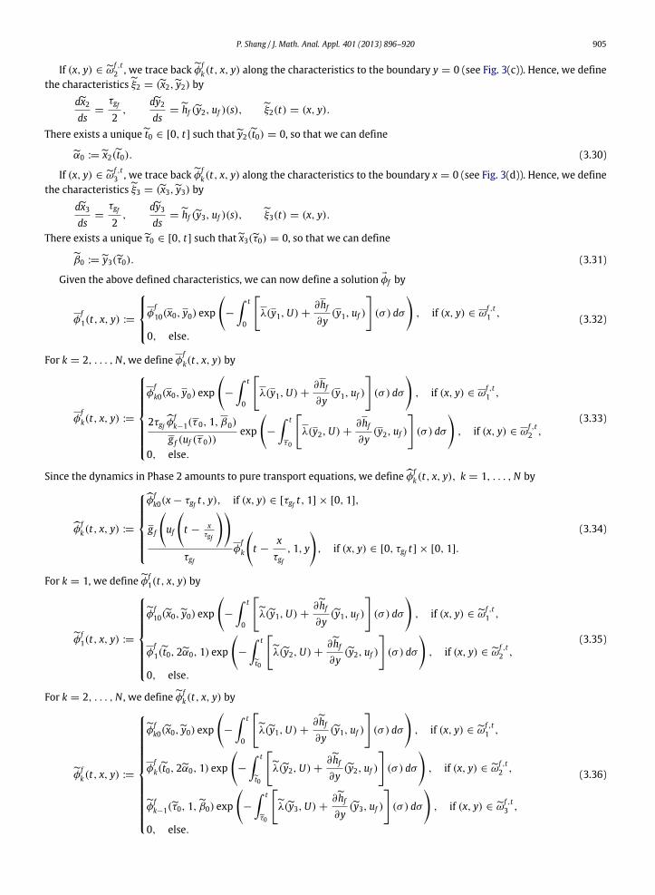
Given the above defined characteristics, we can now define a solution φf by
φf1(t, x, y) :=
φf10(x0, y0) exp
−
t
0
λ(y1,U) +
∂hf
∂y(y1, uf )
(σ ) dσ
, if (x, y) ∈ ω
f ,t1 ,
0, else.(3.32)
For k = 2, . . . ,N , we define φfk(t, x, y) by
φfk(t, x, y) :=
φfk0(x0, y0) exp
−
t
0
λ(y1,U) +
∂hf
∂y(y1, uf )
(σ ) dσ
, if (x, y) ∈ ω
f ,t1 ,
2τgfφfk−1(τ 0, 1, β0)
g f (uf (τ 0))exp
−
t
τ0
λ(y2,U) +
∂hf
∂y(y2, uf )
(σ ) dσ
, if (x, y) ∈ ω
f ,t2 ,
0, else.
(3.33)
Since the dynamics in Phase 2 amounts to pure transport equations, we defineφfk(t, x, y), k = 1, . . . ,N by
906 P. Shang / J. Math. Anal. Appl. 401 (2013) 896–920
Next we prove that the function φf defined by (3.32)–(3.36) is a weak solution to the Cauchy problem (1.2), (1.5)–(1.12)for t ∈ [0, δ]. We first prove that φf satisfies equality (2.5) of Definition 2.1, then we prove that φf ∈ C0([0, δ]; L1((0, 1)2)).
Let τ ∈ [0, δ] and a vector function ϕ(t, x, y) ∈ C1([0, τ ] × [0, 1]2) be given, with
such that (2.1)–(2.4) hold. Using definitions (3.32)–(3.36) of φf , we get
τ
0
1
0
1
0φf (t, x, y) ·
ϕt + Af ϕx + Bf ϕy + C ϕ
dxdydt :=
7i=1
Ai. (3.37)
In (3.37),
A1 :=
Nk=1
τ
0
ωf ,t1
φfk0(x0, y0) exp
−
t
0
λ(y1,U) +
∂hf
∂y(y1, uf )
(σ )dσ
·
ϕkt(t, x, y) + g f ϕkx(t, x, y) + hf ϕky(t, x, y) − λϕk(t, x, y)
dxdydt,
A2 :=
Nk=2
τ
0
ωf ,t2
2τgfφfk−1(τ 0, 1, β0)
g f (uf (τ 0))exp
−
t
τ0
λ(y2,U) +
∂hf
∂y(y2, uf )
(σ )dσ
·
ϕkt(t, x, y) + g f ϕkx(t, x, y) + hf ϕky(t, x, y) − λϕk(t, x, y)
dxdydt,
A3 :=
Nk=1
τ
0
1
0
1
τgf t
φfk0(x − τgf t, y)
ϕkt(t, x, y) + τgfϕkx(t, x, y)dxdydt,
A4 :=
Nk=1
τ
0
1
0
τgf t
0g f
uf
t −
xτgf
φ
fk
t −
xτgf
, 1, y
ϕkt(t, x, y) + τgfϕkx(t, x, y)dxdydt,
A5 :=
Nk=1
τ
0
ωf ,t1
φfk0(x0,y0) exp
−
t
0
λ(y1,U) +∂hf
∂y(y1, uf )
(σ )dσ
·
ϕkt(t, x, y) +τgf
2ϕkx(t, x, y) +hfϕky(t, x, y) −λϕk(t, x, y)
dxdydt,
A6 :=
Nk=1
τ
0
ωf ,t2
φfk(t0, 2α0, 1) exp
−
t
t0λ(y2,U) +
∂hf
∂y(y2, uf )
(σ )dσ
·
ϕkt(t, x, y) +τgf
2ϕkx(t, x, y) +hfϕky(t, x, y) −λϕk(t, x, y)
dxdydt,
A7 :=
Nk=2
τ
0
ωf ,t3
φfk−1(τ0, 1,β0) exp
−
t
τ0λ(y3,U) +
∂hf
∂y(y3, uf )
(σ )dσ
·
ϕkt(t, x, y) +τgf
2ϕkx(t, x, y) +hfϕky(t, x, y) −λϕk(t, x, y)
dxdydt.
Next we prove that equality (2.5) of Definition 2.1 holds by applying the change of variables.We consider the first term A1 as an instance. Let us recall the definition of the characteristic curve ξ 1 = (x1, y1) (see
Fig. 4(a)). Thanks to (C.1) of Lemma C.1 in Appendix C, after applying the change of variables (x, y) → (x0, y0), we get
A1 =
Nk=1
τ
0
β
0
α
0φ
fk0(x0, y0) exp
−
t
0λ(y1,U)(σ )dσ
ϕktt, x1(t), y1(t)
+ g f ϕkx
t, x1(t), y1(t)
+ hf ϕky
t, x1(t), y1(t)
− λϕk
t, x1(t), y1(t)
dx0dy0dt,
where, for any fixed t ∈ [0, τ ], α and β are defined as (see Fig. 4(a))
α := 1 −
t
0g f (uf (σ )) dσ , f1(t), β := 1 −
t
0hf (Γ , uf )(σ )dσ , g1(t). (3.38)
P. Shang / J. Math. Anal. Appl. 401 (2013) 896–920 907
a b
Fig. 4. Illustration of the new integral domains after changing the order of some integrals. (a) For any fixed t ∈ [0, τ ], both the characteristic curve ξ 1(blue) and points (α, 0) and (0, β) are shown. (b) New integral domain in the x0, y0 and τ space after changing the order of integration in term A1 fromdx0dy0dt to dtdx0dy0 . The green surface represents α = f1(t) and the blue surface represents β = g1(t). (For interpretation of the references to colour inthis figure legend, the reader is referred to the web version of this article.)
Clearly,α is a function ofβ , suppose thatα = h(β). After changing the order of integration (see Fig. 4(b)), A1 can be rewrittenas
908 P. Shang / J. Math. Anal. Appl. 401 (2013) 896–920
Note that
x1(f −11 (α)) = y1(g
−11 (β)) = 1. (3.42)
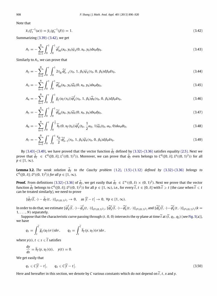
Summarizing (3.39)–(3.42), we get
A1 = −
Nk=1
1
0
1
0φ
fk0(x0, y0)ϕk(0, x0, y0)dx0dy0. (3.43)
Similarly to A1, we can prove that
A2 = −
Nk=2
τ
0
1
02τgfφf
k−1(τ0, 1, β0)ϕk(τ0, 0, β0)dβ0dτ0, (3.44)
A3 = −
Nk=1
1
0
1
0
φfk0(x0, y0)ϕk(0, x0, y0)dx0dy0, (3.45)
A4 = −
Nk=1
τ
0
1
0g f (uf (τ0))φ
fk(τ0, 1, β0)φk(τ0, 0, β0)dβ0dτ0, (3.46)
A5 = −
Nk=1
1
0
1
0
φfk0(x0, y0)ϕk(0, x0, y0)dx0dy0, (3.47)
A6 = −
Nk=1
τ
0
12
0
hf (0, uf (t0))φfk(t0,
12α0, 1)ϕk(t0, α0, 0)dα0dt0, (3.48)
A7 = −
Nk=2
τ
0
1
0
τgf
2φf
k−1(τ0, 1, β0)ϕk(τ0, 0, β0)dβ0dτ0. (3.49)
By (3.43)–(3.49), we have proved that the vector function φf defined by (3.32)–(3.36) satisfies equality (2.5). Next weprove that φf ∈ C0([0, δ]; L1((0, 1)2)). Moreover, we can prove that φf even belongs to C0([0, δ]; Lp((0, 1)2)) for allp ∈ [1, ∞).
Lemma 3.2. The weak solution φf to the Cauchy problem (1.2), (1.5)–(1.12) defined by (3.32)–(3.36) belongs toC0([0, δ]; Lp((0, 1)2)) for all p ∈ [1, ∞).
Proof. From definitions (3.32)–(3.36) of φf , we get easily that φf ∈ L∞((0, δ) × (0, 1)2). Next we prove that the vectorfunction φf belongs to C0([0, δ]; Lp((0, 1)2)) for all p ∈ [1, ∞), i.e., for everyt, t ∈ [0, δ] witht > t (the case whent 6 tcan be treated similarly), we need to prove
∥φf (t, ·) − φf (t, ·)∥Lp((0,1)2) → 0, ast − t
→ 0, ∀p ∈ [1, ∞).
In order to do that, we estimate ∥φfk(t, ·)−φ
fk(t, ·)∥Lp((0,1)2), ∥
φfk(t, ·)−φf
k(t, ·)∥Lp((0,1)2) and ∥φfk(t, ·)−φf
k(t, ·)∥Lp((0,1)2)(k =
1, . . . ,N) separately.Suppose that the characteristic curve passing through (t, 0, 0) intersects the xy plane at timet at (t, q1, q2) (see Fig. 5(a)),
we have
q1 =
tt
g f (uf (σ ))dσ , q2 =
tt
hf (y, uf )(σ )dσ ,
where y(s), t 6 s 6t satisfiesdyds
= hf (y, uf )(s), y(t) = 0.
We get easily that
q1 6 Ct − t
, q2 6 Ct − t
. (3.50)
Here and hereafter in this section, we denote by C various constants which do not depend ont, t, x and y.
P. Shang / J. Math. Anal. Appl. 401 (2013) 896–920 909
Let S := [q1, 1] × [q2, 1] (see Fig. 5(a)). For any fixed (x, y) ∈ S, we define a new characteristic curve ξ 3 = (x3, y3)passing through (t, x, y) that intersects the xy plane at time t at (t,x,y). Then we haveφf
k(t, x, y) − φfk(t, x, y)
=
φfk(t,x,y) exp
−
tt
λ(y3,U) +
∂hf
∂y(y3, uf )
(σ ) dσ
− φ
fk(t, x, y)
6φf
k(t,x,y) − φfk(t, x, y)
exp−
tt
λ(y3,U) +
∂hf
∂y(y3, uf )
(σ ) dσ
+ C
φfk(t, x, y)
t − t.
Furthermore,
x = x −
tt
g f (uf (σ ))dσ , y = y −
tt
hf (y3, uf )(σ )dσ .
Hence, we getx − x 6 C
t − t, y − y
6 Ct − t
. (3.51)
Sinceφfk ∈ L∞((0, δ)×(0, 1)2), for every l > 0, there exists Cl such that for every t ∈ [0, δ], there existsφ
flk(t, ·) ∈ C1([0, 1]2)
satisfying
∥φflk(t, ·) − φ
fk(t, ·)∥Lp((0,1)2) 6
1l, ∥φ
flk(t, ·)∥C1([0,1]2) 6 Cl. (3.52)
Here and hereafter in this section, we denote by Cl various constants that may depend on l (the index of the correspondingapproximating sequences φ
flk(t, ·),φfl
k (t, ·) andφflk (t, ·)) but are independent of 0 6 t 6t 6 δ.
Noting (3.51), we haveφfk(t, x, y) − φ
fk(t, x, y)
6 Cφfl
k(t,x,y) − φfk(t,x,y)+ C
φflk(t, x, y) − φ
fk(t, x, y)
+ C
φfk(t, x, y)
t − t+ Cl
t − t. (3.53)
By (3.52) and (3.53), we getS
φfk(t, x, y) − φ
fk(t, x, y)
pdxdy 6Clp
+ Clt − t
p. (3.54)
Noting (3.50), we have[0,1]2\S
φfk(t, x, y) − φ
fk(t, x, y)
pdxdy 6 C(q1 + q2) 6 Ct − t
. (3.55)
Combining (3.54) with (3.55), we obtain 1
0
1
0
φfk(t, x, y) − φ
fk(t, x, y)
pdxdy 6Clp
+ Clt − t
p + Ct − t
. (3.56)
Next we estimate ∥φfk(t, ·) −φf
k(t, ·)∥Lp((0,1)2). In Phase 2, it is easy to get that the characteristic curve passing through(t, 0, 0) intersects the xy plane at timet at (t, τgf (t − t), 0). LetS := [τgf (t − t), 1] × [0, 1] (see Fig. 5(b)). For any fixed(x, y) ∈S, we haveφf
k(t, x, y) −φfk(t, x, y)
=φf
k(t,x,y) −φfk(t, x, y)
=φf
k(t, x − τgf (t − t), y) −φfk(t, x, y)
.Sinceφf
k ∈ L∞((0, δ)×(0, 1)2), for every l > 0, there exists Cl such that for every t ∈ [0, δ], there existsφflk (t, ·) ∈ C1([0, 1]2)
satisfying
∥φflk (t, ·) −φf
k(t, ·)∥Lp((0,1)2) 61l, ∥φfl
k (t, ·)∥C1([0,1]2) 6 Cl. (3.57)
Similarly to (3.54), we can prove thatSφf
k(t, x, y) −φfk(t, x, y)
pdxdy 6Clp
+ Clt − t
p. (3.58)
910 P. Shang / J. Math. Anal. Appl. 401 (2013) 896–920
a b c
Fig. 5. The xy plane at different time corresponding to each cell cycle k: the xy plane at timet and t with 0 6 t 6t 6 δ. (a) In Phase 1, the characteristiccurve ξ 3 (blue) connects (t, x, y) with (t,x,y) and the characteristic curve (red) passing through (t, 0, 0) intersects the xy plane at timet at (t, q1, q2), sothat we can define the (shaded) domain S. (b) In Phase 2, the characteristic curve (blue) connects (t, x, y) with (t,x,y) and the characteristic curve (red)passing through (t, 0, 0) intersects the xy plane at timet at (t, τgf (t − t), 0), so that we can define the (shaded) domainS. (c) In Phase 3, the characteristiccurveξ4 (blue) connects (t, x, y) with (t,x,y) and the characteristic curve (red) passing through (t, 0, 0) intersects the xy plane at timet at (t, v, v1) andthe characteristic curve (green) passing through (t, 0, 1) intersects the xy plane at timet at (t, v, v2), so that we can define the (shaded) domainS. (Forinterpretation of the references to colour in this figure legend, the reader is referred to the web version of this article.)
It is easy to check that[0,1]2\S
φfk(t, x, y) −φf
k(t, x, y)pdxdy 6 C
t − t. (3.59)
Combining (3.58) with (3.59), we get 1
0
1
0
φfk(t, x, y) −φf
k(t, x, y)pdxdy 6
Clp
+ Clt − t
p + Ct − t
. (3.60)
Finally, we estimate ∥φfk(t, ·)−φf
k(t, ·)∥Lp((0,1)2). Suppose that the characteristic curve passing through (t, 0, 0) intersectsthe xy plane at timet at (t, v, v1), and the characteristic curve passing through (t, 0, 1) intersects the xy plane at timet at(t, v, v2) (see Fig. 5(c)). Similarly to (3.50), we can prove that
v 6 Ct − t
, v1 6 Ct − t
, 1 − v2 6 Ct − t
. (3.61)
LetS := [v, 1] × [v1, v2] (see Fig. 5(c)). For any fixed (x, y) ∈ S, we define the characteristic curveξ4 = (x4,y4) passingthrough (t, x, y) that intersects the xy plane at time t at (t,x,y). Then we have
φfk(t, x, y) −φf
k(t, x, y) =
φfk(t,x,y) exp
−
tt
λ(y4,U) +∂hf
∂y(y4, uf )
(σ )dσ
−φf
k(t, x, y)
.Similarly to (3.51), we can prove thatx − x
6 Ct − t
, y − y 6 C
t − t.
Sinceφfk ∈ L∞((0, δ)×(0, 1)2), for every l > 0, there exists Cl such that for every t ∈ [0, δ], there existsφfl
k (t, ·) ∈ C1([0, 1]2)satisfying
∥φflk (t, ·) −φf
k(t, ·)∥Lp((0,1)2) 61l, ∥φfl
k (t, ·)∥C1([0,1]2) 6 Cl. (3.62)
Similarly to (3.54), we can prove thatSφf
k(t, x, y) −φfk(t, x, y)
pdxdy 6Clp
+ Clt − t
p. (3.63)
Noting (3.61), we have[0,1]2\S
φfk(t, x, y) −φf
k(t, x, y)pdxdy 6 C(v + v1 + 1 − v2) 6 C
t − t. (3.64)
P. Shang / J. Math. Anal. Appl. 401 (2013) 896–920 911
Combining (3.63) with (3.64), we get 1
0
1
0
φfk(t, x, y) −φf
k(t, x, y)pdxdy 6
Clp
+ Clt − t
p + Ct − t
. (3.65)
Therefore letting l be large enough and then |t − t| be small enough, the right hand side of (3.56), (3.60) and (3.65)can be arbitrarily small. As a whole, we have proved that the vector function φf belongs to C0([0, δ]; Lp((0, 1)2)) for allp ∈ [1, ∞).
Let us recall Definition 2.1 of a weak solution, we have proved that the vector function φf defined by (3.32)–(3.36) isindeed a weak solution to the Cauchy problem (1.2), (1.5)–(1.12).
4. Uniqueness of the solution
In this section,we prove the uniqueness of theweak solution, the proof is inspired from [6,16]. By solving a correspondingbackward linear Cauchy problem, we first prove that the twomaturities corresponding to two different solutions satisfy thesame contractionmapping function Gdefined by (3.7). By the uniqueness of the fixedpoint that determines the characteristiccurves, it then follows the uniqueness of the weak solution.
Lemma 4.1. The weak solution to the Cauchy problem (1.2), (1.5)–(1.12) is unique.
Proof. Assume that φf =φ
f
1, . . . , φf
N ,φf
1, . . . ,φf
N ,φf
1, . . . ,φf
N
T∈ C0([0, δ]; L1((0, 1)2)) is another weak solution to the
Cauchy problem (1.2), (1.5)–(1.12). Similarly to Lemma 2.2 in [6, Section 2.2], we can prove that for any fixed t ∈ [0, δ] andany Φ(τ , x, y) :=
Let us recall the simplified notation uf = uf (Mf ,M, t) and uf = uf (M f ,M, t). For any fixed t ∈ [0, δ], we define three newsubsets ω
f ,t1 , ω
f ,t2 and ω
f ,t3 of [0, 1]2 in the same way as in (3.19)–(3.21), but with uf instead of uf .
For any fixed t ∈ [0, δ] and (x, y) ∈ [0, 1]2, if (x, y) ∈ ωf ,t1 , we define ξ 1 = (x1, y1) by
dx1ds
= g f (uf (s)),dy1ds
= hf (y1, uf )(s), ξ 1(t) = (x, y). (4.3)
912 P. Shang / J. Math. Anal. Appl. 401 (2013) 896–920
Let us then define
(x0, y0) := (x1(0), y1(0)). (4.4)
If (x, y) ∈ ωf ,t2 , we define ξ 2 = (x2, y2) by
dx2ds
= g f (uf (s)),dy2ds
= hf (y2, uf )(s), ξ 2(t) = (x, y).
There exists a unique τ 0 such that x2(τ 0) = 0, so that we can define
β0 := y2(τ 0). (4.5)
Combining (4.1) with (4.2), we obtain that 1
0
1
0φf (t, x, y) · Φ(t, x, y)dxdy =
1
0
1
0φf (t, x, y) · ϕ0(x, y)dxdy
=
1
0
1
0φf 0(x, y) · Φ(0, x, y)dxdy (4.6)
+
Nk=1
t
0
12
0
hf (0, uf (τ ))φf
k(τ , 2x, 1)Φk(τ , x, 0)dxdτ (4.7)
+
Nk=2
t
0
1
02τgfφf
k−1(τ , 1, y)Φk(τ , 0, y)dydτ (4.8)
+
Nk=2
t
0
1
0
τgf
2φf
k−1(τ , 1, y)Φk(τ , 0, y)dydτ (4.9)
+
Nk=1
t
0
1
0g f (uf (τ ))φ
f
k(τ , 1, y)Φk(τ , 0, y)dydτ . (4.10)
For the last term (4.10), since Φk satisfy pure transport equations, by solving the backward linear Cauchy problem (4.2), weget that (4.10) becomes
Nk=1
1
0
τgf t
0
g f
uf
t −
xτgf
τgf
φf
k
t −
xτgf
, 1, y
ϕ0k(x, y)dxdy. (4.11)
Let us recall definition (4.3) of the characteristic curve ξ 1 and also definition (4.4) of (x0, y0). By solving the backward linearCauchy problem (4.2) and noting (C.1) of Lemma C.1 in Appendix C, we get that (4.6) becomes
Nk=1
ωf ,t1
φfk0(x0, y0)ϕ0k(x, y) exp
−
t
0
λ(y1,U) +
∂hf
∂y(y1, uf )
(σ ) dσ
dxdy
+
1
0
1
t
φfk0(x − τgf t, y)ϕ0k(x, y)dxdy +
Nk=1
1
0
1
0
φfk0(x, y)Φk(0, x, y)dxdy. (4.12)
Since ϕ0 ∈ C10 ((0, 1)2) and t ∈ [0, δ] are both arbitrary, from (4.11) and (4.12), we obtain in C0([0, δ]; L1((0, 1)2)) that for
P. Shang / J. Math. Anal. Appl. 401 (2013) 896–920 913
Let us recall the definition of the characteristic curve ξ 2 and also definition (4.5) of (τ 0, β0). By solving the backward linearCauchy problem (4.2), noting (4.13) and (C.2) of Lemma C.1 in Appendix C, we get that (4.8) becomes
Nk=2
ωf ,t2
2τgfφfk−1(τ 0, 1, β0)
g f (uf (τ 0))ϕ0k(x, y) exp
−
t
τ0
λ(y2,U) +
∂hf
∂y(y2, uf )
(σ ) dσ
dxdy. (4.14)
Since ϕ0 ∈ C10 ((0, 1)2) and t ∈ [0, δ] are both arbitrary, from (4.12) and (4.14), we obtain in C0([0, δ]; L1((0, 1)2)) that for
k = 1
φf
1(t, x, y) =
φf10(x0, y0) exp
−
t
0
λ(y1,U) +
∂hf
∂y(y1, uf )
(σ ) dσ
, if (x, y) ∈ ω
f ,t1 ,
0, else.(4.15)
For k = 2, . . . ,N , we have
φf
k(t, x, y) =
φ
fk0(x0, y0) exp
−
t
0
λ(y1,U) +
∂hf
∂y(y1, uf )
(σ ) dσ
, if (x, y) ∈ ω
f ,t1 ,
2τgfφfk−1(τ 0, 1, β0)
g f (uf (τ 0))exp
−
t
τ0
λ(y2,U) +
∂hf
∂y(y2, uf )
(σ ) dσ
, if (x, y) ∈ ω
f ,t2 ,
0, else.
(4.16)
For any fixed t ∈ [0, δ], we define four new subsetsωf ,t1 ,ωf ,t
2 ,ωf ,t3 andωf ,t
4 of [0, 1]2 in the same way as in (3.25)–(3.28),but with uf instead of uf .
For any fixed t ∈ [0, δ] and (x, y) ∈ [0, 1]2, if (x, y) ∈ ωf ,t1 , we defineξ 1 = (x1,y1) by
dx1ds
=τgf
2,
dy1ds
=hf (y1, uf )(s), ξ 1(t) = (x, y).
Let us then define (x0,y0) := (x1(0),y1(0)). With this definition, we solve the backward linear Cauchy problem (4.2) anduse (C.3) of Lemma C.1 in Appendix C, the last term in (4.12) can be rewritten as
Nk=1
ωf ,t1
φfk0(x0,y0)ϕ0k(x, y) exp
−
t
0
λ(y1,U) +
∂hf
∂y(y1, uf )
(σ ) dσ
dxdy. (4.17)
If (x, y) ∈ ωf ,t2 , we defineξ 2 = (x2,y2) by
dx2ds
=τgf
2,
dy2ds
=hf (y2, uf )(s), ξ 2(t) = (x, y).
There exists a uniquet0 such thaty2(t0) = 0, so that we can defineα0 :=x2(t0). With this definition, we solve the backwardlinear Cauchy problem (4.2) and use (C.4) of Lemma C.1 in Appendix C, we get that (4.7) becomes
Nk=1
ωf ,t2
φf
k(t0, 2α0, 1)ϕ0k(x, y) exp
−
t
t0λ(y2,U) +
∂hf
∂y(y2, uf )
(σ ) dσ
dxdy. (4.18)
If (x, y) ∈ ωf ,t3 , we defineξ 3 = (x3,y3) by
dx3ds
=τgf
2,
dy3ds
=hf (y3, uf )(s), ξ 3(t) = (x, y).
There exists a uniqueτ 0 such thatx3(τ 0) = 0, so that we can define β0 := y3(τ 0). With this definition, we solve thebackward linear Cauchy problem (4.2) and use (C.5) of Lemma C.1 in Appendix C, we get that (4.9) becomes
Nk=2
ωf ,t3
φf
k−1(τ 0, 1,β0)ϕ0k(x, y) exp
−
t
τ0
λ(y3,U) +∂hf
∂y(y3, uf )
(σ ) dσ
dxdy. (4.19)
Since ϕ0 ∈ C10 ((0, 1)2) and t ∈ [0, δ] are both arbitrary, combining (4.12) and (4.17)–(4.19), we obtain in C0([0, δ];
L1((0, 1)2)) that for k = 1
914 P. Shang / J. Math. Anal. Appl. 401 (2013) 896–920
φf
1(t, x, y) =
φf10(x0,y0) exp
−
t
0
λ(y1,U) +∂hf
∂y(y1, uf )
(σ ) dσ
, if (x, y) ∈ ωf ,t
1 ,
φf
1(t0, 2α0, 1) exp
−
t
t0λ(y2,U) +
∂hf
∂y(y2, uf )
(σ ) dσ
, if (x, y) ∈ ωf ,t
2 ,
0, else.
(4.20)
For k = 2, . . . ,N , we get
φf
k(t, x, y) =
φfk0(x0,y0) exp
−
t
0
λ(y1,U) +∂hf
∂y(y1, uf )
(σ ) dσ
, if (x, y) ∈ ωf ,t
1 ,
φf
1(t0, 2α0, 1) exp
−
t
t0λ(y2,U) +
∂hf
∂y(y2, uf )
(σ ) dσ
, if (x, y) ∈ ωf ,t
2 ,
φf
k−1(τ 0, 1,β0) exp
−
t
τ0
λ(y3,U) +∂hf
∂y(y3, uf )
(σ ) dσ
, if (x, y) ∈ ωf ,t
3 ,
0, else.
(4.21)
By (3.9), we claim that M(t) = (M1, . . . ,Mn) ∈ Ωδ, K and M(t) satisfies the same contraction mapping function G
defined by (3.7). Since M is the unique fixed point of G in Ωδ, K , we have M ≡ M . Consequently, we have ξ i ≡ ξ i (i =
1, 2),ξ i = ξi (i = 1, 2, 3),ηi ≡ ηi(i = 1, 2) and η ≡ η. Obviously, we have then (x0, y0) ≡ (x0, y0), (x0,y0) ≡ (x0,y0),(t0,α0) ≡ (t0,α0), (τ 0, β0) ≡ (τ 0, β0), (τ 0,β0) ≡ (τ0,β0), ω
f ,ti ≡ ω
f ,ti (i = 1, 2, 3) and ωf ,t
i ≡ ωf ,ti (i = 1, 2, 3, 4).
Finally, by comparing definitions (4.13), (4.15)–(4.16) and (4.20)–(4.21) of φf with definitions (3.32)–(3.36) of φf , we obtain
φf ≡ φf . This gives us the uniqueness of the weak solution for small time.
5. Proof of the existence of a global solution to the Cauchy problem
Let us now prove the existence of global solution to the Cauchy problem (1.2), (1.5)–(1.12). By definition (3.8) of Gf anddefinitions (3.32)–(3.36) of the local solution φf , it is easy to check that the following two estimates hold for all t ∈ [0, δ]
0 6 M(t) 6 K , (5.1)
∥φf (t, ·)∥L∞((0,1)2) 6 exp2(N + 1)TK1
max
k
2 K1
K2+
K1
τgf
N
∥φfk0∥,
2(K1 + τgf )
K2
N
∥φfk0∥, ∥
φfk0∥
, (5.2)
where K is defined by (3.1), K1 is defined by (3.2) and K2 is defined by (3.3). In order to obtain a global solution, wesuppose that we have solved the Cauchy problem (1.2), (1.5)–(1.12) up to the moment τ ∈ [0, T ] with the weak solutionφf ∈ C0([0, τ ]; Lp((0, 1)2)). Fromourway to construct theweak solution, we know that for any 0 6 t 6 τ , theweak solutionis given in the form defined by (3.32)–(3.36).
As time increases, for each cell cycle k (k = 1, . . . ,N) in Phase 1, the characteristic curvewhich passes through the originmay encounter two possible cases. It may either intersect with the front face (see Fig. 6(a)), then go to Phase 2 (mitosis). Orit may intersect with the right face (see Fig. 6(b)), then go to Phase 3 (differentiation). For each cell cycle k (k = 1, . . . ,N)in Phase 3, the characteristic curve which passes through the origin will definitely intersect with the front face due to theassumption thathf (1, uf ) < 0 (see Fig. 6(c)). Then it will go further to the next cell cycle. We get in any case that
Mf (t) :=
Nk=1
ωf ,t2
γ 2s yφ
fk(t, x, y)dxdy +
Nk=1
1
0
1
0γ 2s yφf
k(t, x, y)dxdy
+
Nk=1
ωf ,t2 ∪ ωf ,t
3
2γdγdy + γs
φfk(t, x, y)dxdy.
Thanks to Lemma C.1 in Appendix C, after tracing back φfk(t, x, y),φf
k(t, x, y) and φfk(t, x, y) along the characteristics
finally to the initial data at most N times, we can prove that estimate (5.1) holds for every t ∈ [0, T ]. Moreover, notingdefinitions (3.32)–(3.36) of the global solution, it is easy to check that the uniform a priori estimate (5.2) holds for everyt ∈ [0, T ]. Hence we can choose δ ∈ [0, T ] independent of τ . Applying Lemmas 3.2 and 4.1 again, the weak solutionφf ∈ C0([0, τ ]; Lp((0, 1)2)) can be extended to the time interval [τ , τ + δ] ∩ [τ , T ]. Step by step, we finally obtain a uniqueglobal weak solution φf ∈ C0([0, T ]; Lp((0, 1)2)) for any p ∈ [1, ∞). This finishes the proof of the existence of a globalsolution to the Cauchy problem (1.2), (1.5)–(1.12).
P. Shang / J. Math. Anal. Appl. 401 (2013) 896–920 915
a b c
Fig. 6. Division of the xy plane at time t , for each cell cycle k when t is large enough. In Phase 1, when t is large, the characteristic curve (red) passingthrough the origin may encounter two cases: in case (a), it intersects the front face, then go to Phase 2; in case (b), it intersects the right face, then go toPhase 3. (c) In Phase 3, due to the assumption thathf (1, uf ) < 0, the characteristic curve (red) passing through the origin will definitely intersect the frontface, then go to the next cycle k + 1. (For interpretation of the references to colour in this figure legend, the reader is referred to the web version of thisarticle.)
Remark 5.1. The characteristic curves cannot intersect on the whole set [0, 1]2 for each t , since we assume that theregularity of the velocity functions hf (y, uf ) is C1 with respect to space y. The values of the velocity functions do not dependdirectly on the solution but only on the integral of the solution. Since the velocity functions hf (y, uf ) are Lipschitz continuouswith respect to space y, we have the uniqueness of the characteristic curves at each (t, x, y) for any t ∈ [0, T ].
Acknowledgments
The author would like to thank the professors Frédérique Clément, Jean-Michel Coron and Zhiqiang Wang for theirinteresting comments and many valuable suggestions on this work. PS was supported by the INRIA large scale initiativeaction REGATE (REgulation of the GonAdoTropE axis) and by the ERC advanced grant 266907 (CPDENL) of the 7th ResearchFramework Programme (FP7).
Appendix A. Introduction of the model
In this section, we first recall the system of equations describing the dynamics of the cell density of ovarian follicles inthemodel of F. Clément [4,7,8]. The cell population in a follicle f is represented by cell density functions φ
fj,k(t, a, γ ) defined
on each cellular phase Q fj,k with age a and maturity γ , which satisfy the following conservation laws
∂φfj,k
∂t+
∂(gf (uf )φfj,k)
∂a+
∂(hf (γ , uf )φfj,k)
∂γ= −λ(γ ,U)φ
fj,k, in Q f
j,k (A.1)
Q fj,k := Σj,k × [0, T ], for j = 1, 2, 3, f = 1, . . . , n, where
Here k = 1, . . . ,N , and N is the number of consecutive cell cycles (see Fig. A.7).Define the maturity operatorM as
M(ϕ)(t) :=
γm
0
am
0γ ϕ(t, a, γ ) dadγ . (A.2)
Then
Mf :=
3j=1
Nk=1
γm
0
am
0γφ
fj,k(t, a, γ ) dadγ (A.3)
is the global follicular maturity on the follicular scale, while
M :=
nf=1
3j=1
Nk=1
γm
0
am
0γφ
fj,k(t, a, γ ) dadγ (A.4)
is the global maturity on the ovarian scale.
916 P. Shang / J. Math. Anal. Appl. 401 (2013) 896–920
Fig. A.7. Domain of the solution in the original model. For each follicle f , the domain consists of the sequence of N cell cycles. a denotes the age of the celland γ denotes its maturity. The top of the domain corresponds to the differentiation phase and the bottom to the proliferation phase.
In (A.2)–(A.4), γm and am are maximum of maturity and age. The velocity and source terms are all smooth functions ofuf and U , where uf is the local control and U is the global control. In this paper, we consider both closed and open loopproblems, that is to say uf and U are functions ofMf ,M and t . As an instance of closed loop problem, the velocity and sourceterms are given by the following expressions in [4] (all parameters are positive constants)
gf (uf ) = τgf (1 − g1(1 − uf )), in Σ1,k,
gf (uf ) = τgf , in Σj,k, j = 2, 3,
hf (γ , uf ) = τhf
−γ 2
+ (c1γ + c2)
1 − exp
−uf
u
, in Σj,k, j = 1, 3, (A.5)
hf (γ , uf ) = λ(γ ,U) = 0, in Σ2,k,
λ(γ ,U) = K exp
−
γ − γs
γ
2(1 − U), in Σj,k, j = 1, 3,
U = S(M) + U0 = U0 + Us +1 − Us
1 + expc(M − m)
,uf = b(Mf )U = min
b1 +
expb2Mf
b3
, 1
·
U0 + Us +
1 − Us
1 + expc(M − m)
.
The initial conditions are given as follows
φfj,k(0, a, γ ) = φ
fk0(a, γ )|Σj,k , j = 1, 2, 3. (A.6)
The boundary conditions are given as follows
gf (uf )φf1,k
t, (k − 1)a2, γ
=
2τgf φ
f2,k−1
t, (k − 1)a2, γ
, for k > 2,
0, for k = 1,for γ ∈ [0, γs],
φf1,k
t, a, 0
= 0, for a ∈ [(k − 1)a2, (k − 1)a2 + a1],
τgf φf2,k
t, (k − 1)a2 + a1, γ
= gf (uf )φ
f1,k
t, (k − 1)a2 + a1, γ
, for γ ∈ [0, γs],
φf2,k
t, a, 0
= 0, for a ∈ [(k − 1)a2 + a1, ka2],
φf3,k
t, (k − 1)a2, γ
=
φ
f3,k−1
t, (k − 1)a2, γ
, for k > 2,
0, for k = 1,for γ ∈ [γs, γm],
φf3,k
t, a, γs
=
φ
f1,k
t, a, γs
, for a ∈ [(k − 1)a2, (k − 1)a2 + a1],
0, for a ∈ [(k − 1)a2 + a1, ka2].
Appendix B. Mathematical reformulation
In this section, we perform amathematical reformulation of the original model introduced in Appendix A. One can noticethat in system (A.1), all the unknowns are defined on different domains, so that one has to solve the equations successively.Here we transform system (A.1) into a regular one where the unknowns are defined on the same domain [0, T ] × [0, 1]2. InPhase 1, we denote by φ
fk the density functions, g f the age velocities and hf the maturity velocities. In Phase 2, we denote
P. Shang / J. Math. Anal. Appl. 401 (2013) 896–920 917
byφfk the density functions andgf the age velocities. In Phase 3, we denote byφf
k the density functions,gf the age velocitiesandhf the maturity velocities.
Let
φfk(t, x, y) := φ
f1,k(t, a, γ ), (a, γ ) ∈ Σ1,k, (B.1)
where
x :=a − (k − 1)a2
a1, y :=
γ
γs, (B.2)
so that we get (a, γ ) ∈ Σ1,k ⇐⇒ (x, y) ∈ [0, 1]2, and
(φfk)t + (g f φ
fk)x + (hf φ
fk)y = −λ φ
fk, (B.3)
with
g f (uf ) :=gf (uf )
a1, hf (y, uf ) :=
hf (γsy, uf )
γs, λ(y,U) := λ(γsy,U). (B.4)
Let φfk(t, x, y) := φ
f2,k(t, a, γ ), (a, γ ) ∈ Σ2,k, (B.5)
where
x :=a − (k − 1)a2 − a1
a2 − a1, y :=
γ
γs. (B.6)
So that we get (a, γ ) ∈ Σ2,k ⇐⇒ (x, y) ∈ [0, 1]2, and
(φfk)t +gf (φf
k)x = 0, gf :=τgf
a2 − a1. (B.7)
Let φfk(t, x, y) := φ
f3,k(t, a, γ ), (a, γ ) ∈ Σ3,k, (B.8)
where
x :=a − (k − 1)a2
a2, y :=
γ − γs
γm − γs, (B.9)
so that we get (a, γ ) ∈ Σ3,k ⇐⇒ (x, y) ∈ [0, 1]2, and
(φfk)t + (gfφf
k)x + (hfφfk)y = −λφf
k, (B.10)
with
gf :=τgf
a2, hf (y, uf ) :=
hf ((γm − γs)y + γs, uf )
γm − γs, λ(y,U) := λ((γm − γs)y + γs,U). (B.11)
Correspondingly, let us denote the initial conditions (A.6) with new notation by
φf 0 :=φ
f10(x, y), . . . , φ
fN0(x, y), φf
10(x, y), . . . ,φfN0,
φf10(x, y), . . . ,φf
N0(x, y), (B.12)
where
φfk0(x, y) := φ
f1,k(0, a, γ ), φf
k0(x, y) := φf2,k(0, a, γ ), φf
k0(x, y) := φf3,k(0, a, γ ). (B.13)
Let φf :=φ
f1, . . . , φ
fN , φf
1, . . . ,φf
N , φf1, . . . ,
φfN
T, we have
φf (t, x, y)t +Af φf (t, x, y)
x +
Bf φf (t, x, y)
y = C φf (t, x, y), t > 0, (x, y) ∈ [0, 1]2, (B.14)
where
Af := diag N g f , . . . , g f ,
N gf , . . . ,gf N gf , . . . ,gf ,Bf := diag
N hf , . . . , hf ,
N 0, . . . , 0
N hf , . . . ,hf
,
C := −diag N λ, . . . , λ,
N 0, . . . , 0
N λ, . . . ,λ.
918 P. Shang / J. Math. Anal. Appl. 401 (2013) 896–920
Without loss of generality, we assume that a1 = a2 − a1 = 1 and γd = γm − γs in the whole paper. Correspondingly, thevelocities become
Finally, we derive the assumptions on maturity velocities hf and hf from the view point of biology. From the originalexpression of hf (γ , uf ) (see (A.5) in Appendix A), let us define
γ±(uf ) :=
c1
1 − exp
−ufu
±
c21
1 − exp
−ufu
2
+ 4c2
1 − exp
−ufu
2
.
It is easy to see that γ+(uf ) is an increasing function of uf , and
hf (γ , uf ) = τhf (γ+(uf ) − γ )(γ − γ−(uf )).
Hence, when γ = γ+(uf ), we have hf (γ , uf ) = 0; moreover
hf (γ , uf ) > 0, if 0 6 γ < γ+(uf ),
hf (γ , uf ) < 0, if γ > γ+(uf ).
Furthermore, under the assumption that the local control uf satisfies γ+(uf ) > γs, we have
0 6 γ+(uf ) 6 γ+(1) ≃
1 − exp
−1u
c1 +
c21 + 4c2
2< γm.
From the fact that 0 < γ 6 γs in Phase 1 and γs 6 γ 6 γm in Phase 3, we have
hf (γ , uf ) > 0, 0 < γ 6 γs,
hf (γs, uf ) > 0, hf (γm, uf ) < 0.
Corresponding to the new notation, we have assumptions
P. Shang / J. Math. Anal. Appl. 401 (2013) 896–920 919
Appendix C. Basic lemmas and some notation
The following lemma is used to prove the existence of the weak solution to the Cauchy problem (1.2), (1.5)–(1.12), whenwe derive the contraction mapping function G, change variables in some integrals (see Section 3) and prove the uniquenessof the solution (see Section 4).
Lemma C.1. The characteristic curve ξ 1 = (x1, y1) passing through (t, x, y) intersects the bottom face at (0, x0, y0). We have
∂(x, y)∂(x0, y0)
= exp
t
0
∂hf
∂y(y1, uf )(σ ) dσ
. (C.1)
The characteristic curve ξ 2 = (x2, y2) passing through (t, x, y) intersects the back face at (τ 0, 0, β0). We have
∂(x, y)
∂(τ 0, β0)= −g f
uf (τ 0)
· exp
t
τ0
∂hf
∂y(y2, uf )(σ ) dσ
. (C.2)
The characteristic curveξ1 = (x1,y1) passing through (t, x, y) intersects the bottom face at (0,x0,y0). We have
∂(x, y)∂(x0,y0) = exp
t
0
∂hf
∂y(y1, uf )(σ ) dσ
. (C.3)
The characteristic curveξ2 = (x2,y2) passing through (t, x, y) intersects the left face at (t0,α0, 0). We have
∂(x, y)∂(t0,α0)
=hf0, uf (t0) · exp
t
t0∂hf
∂y(y2, uf )(σ ) dσ
. (C.4)
The characteristic curveξ3 = (x3,y3) passing through (t, x, y) intersects the back face at (τ0, 0,β0). We have
∂(x, y)
∂(τ0,β0)= −
τgf
2exp
t
τ0∂hf
∂y(y3, uf )(σ ) dσ
. (C.5)
The proof of this lemma is trivial, and can be found in [11] for the one-dimensional case, we omit it here.The expressions of contraction mapping coefficients C f
1 and C f2 are the following
C f1 :=
(γs + γd)2(2 K 2
1 − tK 21 + 3 K1 + tK 2
1 K2 + 9 K1 K2)
K2(1 − tK1)
Nk=1
∥φfk0∥
+2(γs + γd)
2(K 21 + 2tK 2
1 K2 + 4 K1 K2)
K2(1 − tK1)
Nk=2
∥φfk0∥ +
2(γs + γd)2(2 K1 + 2tK 2
1 )
1 − tK1
Nk=1
∥φfk0∥,
C f2 :=
(γs + γd)2(2 K 2
1 + 2 K1 + 12 K1 K2 − 2tK 21 K2)
K2(1 − tK1)
Nk=1
∥φfk0∥
+2(γs + γd)
2(K 21 + 6 K1 K2)
K2(1 − tK1)
Nk=2
∥φfk0∥ +
8(γs + γd)2 K1
1 − tK1∥φf
k0∥. (C.6)
References
[1] D. Armbruster, P. Degond, C. Ringhofer, Amodel for the dynamics of large queuing networks and supply chains, SIAM J. Appl.Math. 66 (2006) 896–920.[2] S. Bianchini, A. Bressan, Vanishing viscosity solutions of nonlinear hyperbolic systems, Ann. of Math. 161 (2005) 223–342.[3] A. Bressan, Hyperbolic Systems of Conservation Laws. The One Dimensional Cauchy Problem, Oxford University Press, Oxford, 2000.[4] F. Clément, Multiscale modelling of endocrine systems: new insight on the gonadotrope axis, ESAIM Proc. 27 (2009) 209–226.[5] J.-M. Coron, Control and Nonlinearity, in: Mathematical Surveys and Monographs, vol. 136, American Mathematical Society, 2007.[6] J.-M. Coron, M. Kawski, Z. Wang, Analysis of a conservation law modeling a highly re-entrant manufacturing system, Discrete Contin. Dyn. Syst. Ser.
B 14 (2010) 1337–1359.[7] N. Echenim, F. Clément, M. Sorine, Multi-scale modeling of follicular ovulation as a reachability problem, Multiscale Model. Simul. 6 (2007) 895–912.[8] N. Echenim, D. Monniaux, M. Sorine, F. Clément, Multi-scale modeling of the follicle selection process in the ovary, Math. Biosci. 198 (2005) 57–79.[9] S.N. Kružkov, First order quasilinear equations in several independent variables, Sb. Math. 10 (1970) 217–243.
[10] T.-T. Li, Global Classical Solutions for Quasilinear Hyperbolic Systems, in: Research in Applied Mathematics, vol. 32, John Wiley & Sons, Chichester,1994.
920 P. Shang / J. Math. Anal. Appl. 401 (2013) 896–920
[11] T.-T. Li, W.C. Yu, Boundary Value Problems for Quasilinear Hyperbolic Systems, in: Duke University Mathematics Series, vol. V, Duke University,Mathematics Department, Durham, NC, 1985.
[12] T.-P. Liu, T. Yang, Well-posedness theory for hyperbolic conservation laws, Comm. Pure Appl. Math. 52 (1999) 1553–1586.[13] E.A. McGee, A.J. Hsueh, Initial and cyclic recruitment of ovarian follicles, Endocr. Rev. 21 (2009) 200–214.[14] P. Michel, Multiscale modeling of follicular ovulation as a mass and maturity dynamical system, Multiscale Model. Simul. 9 (2011) 282–313.[15] A. Poretta, J. Vovelle, l1 solutions to first order hyperbolic equations in bounded domains, Comm. Partial Differential Equations 28 (2003) 381–408.[16] P. Shang, Z. Wang, Analysis and control of a scalar conservation lawmodeling a highly re-entrant manufacturing system, J. Differential Equations 250
(2011) 949–982.[17] J.P. Zhang, A nonlinear nonlocal multi-dimensional conservation law, J. Math. Anal. Appl. 204 (1996) 353–388.[18] K. Zumbrun, On a nonlocal dispersive equation modeling particle suspensions, Quart. Appl. Math. 57 (1999) 573–600.