Causal Time Series Analysis of functional Magnetic Resonance ...

JMLR: Workshop and Conference Proceedings 12 (2011) 65–94 Causality in Time Series

Causal Time Series Analysis of functional MagneticResonance Imaging Data

Alard Roebroeck [email protected] of Psychology & NeuroscienceMaastricht University, the Netherlands

Anil K. Seth [email protected] Centre for Consciousness ScienceUniversity of Sussex, UK

Pedro Valdes-Sosa [email protected]

Cuban Neuroscience Centre, Playa, Cuba

Editor: Florin Popescu and Isabelle Guyon

Abstract

This review focuses on dynamic causal analysis of functional magnetic resonance (fMRI)data to infer brain connectivity from a time series analysis and dynamical systems per-spective. Causal influence is expressed in the Wiener-Akaike-Granger-Schweder (WAGS)tradition and dynamical systems are treated in a state space modeling framework. Thenature of the fMRI signal is reviewed with emphasis on the involved neuronal, physiologi-cal and physical processes and their modeling as dynamical systems. In this context, twostreams of development in modeling causal brain connectivity using fMRI are discussed:time series approaches to causality in a discrete time tradition and dynamic systems andcontrol theory approaches in a continuous time tradition. This review closes with discussionof ongoing work and future perspectives on the integration of the two approaches.

Keywords: fMRI, hemodynamics, state space model, Granger causality, WAGS influence

1. Introduction

Understanding how interactions between brain structures support the performance of spe-cific cognitive tasks or perceptual and motor processes is a prominent goal in cognitiveneuroscience. Neuroimaging methods, such as Electroencephalography (EEG), Magnetoen-cephalography (MEG) and functional Magnetic Resonance Imaging (fMRI) are employedmore and more to address questions of functional connectivity, inter-region coupling andnetworked computation that go beyond the ‘where’ and ‘when’ of task-related activity(Friston, 2002; Horwitz et al., 2000; McIntosh, 2004; Salmelin and Kujala, 2006; Valdes-Sosa et al., 2005a). A network perspective onto the parallel and distributed processingin the brain - even on the large scale accessible by neuroimaging methods - is a promis-ing approach to enlarge our understanding of perceptual, cognitive and motor functions.Functional Magnetic Resonance Imaging (fMRI) in particular is increasingly used not onlyto localize structures involved in cognitive and perceptual processes but also to study theconnectivity in large-scale brain networks that support these functions.

c© 2011 A. Roebroeck, A.K. Seth & P. Valdes-Sosa.

Roebroeck Seth Valdes-Sosa

Generally a distinction is made between three types of brain connectivity. Anatomicalconnectivity refers to the physical presence of an axonal projection from one brain areato another. Identification of large axon bundles connecting remote regions in the brainhas recently become possible non-invasively in vivo by diffusion weighted Magnetic res-onance imaging (DWMRI) and fiber tractography analysis (Johansen-Berg and Behrens,2009; Jones, 2010). Functional connectivity refers to the correlation structure (or moregenerally: any order of statistical dependency) in the data such that brain areas can begrouped into interacting networks. Finally, effective connectivity modeling moves beyondstatistical dependency to measures of directed influence and causality within the networksconstrained by further assumptions (Friston, 1994).Recently, effective connectivity techniques that make use of the temporal dynamics in

the fMRI signal and employ time series analysis and systems identification theory havebecome popular. Within this class of techniques two separate developments have beenmost used: Granger causality analysis (GCA; Goebel et al., 2003; Roebroeck et al., 2005;Valdes-Sosa, 2004) and Dynamic Causal Modeling (DCM; Friston et al., 2003). Despitethe common goal, there seem to be differences between the two methods. Whereas GCAexplicitly models temporal precedence and uses the concept of Granger causality (or G-causality) mostly formulated in a discrete time-series analysis framework, DCM employs abiophysically motivated generative model formulated in a continuous time dynamic systemframework. In this chapter we will give a general causal time-series analysis perspectiveonto both developments from what we have called the Wiener-Akaike-Granger-Schweder(WAGS) influence formalism (Valdes-Sosa et al., in press).Effective connectivity modeling of neuroimaging data entails the estimation of multivari-

ate mathematical models that benefits from a state space formulation, as we will discussbelow. Statistical inference on estimated parameters that quantify the directed influencebetween brain structures, either individually or in groups (model comparison) then providesinformation on directed connectivity. In such models, brain structures are defined from atleast two viewpoints. From a structural viewpoint they correspond to a set of “nodes” thatcomprise a graph, the purpose of causal discovery being the identification of active links inthe graph. The structural model contains i) a selection of the structures in the brain thatare assumed to be of importance in the cognitive process or task under investigation, ii)the possible interactions between those structures and iii) the possible effects of exogenousinputs onto the network. The exogenous inputs may be under control of the experimenterand often have the form of a simple indicator function that can represent, for instance, thepresence or absence of a visual stimulus in the subject’s view. From a dynamical viewpointbrain structures are represented by states or variables that describe time varying neuralactivity within a time-series model of the measured fMRI time-series data. The functionalform of the model equations can embed assumptions on signal dynamics, temporal prece-dence or physiological processes from which signals originate.We start this review by focusing on the nature of the fMRI signal in some detail in

section 2, separating the treatment into neuronal, physiological and physical processes. Insection 3 we review two important formal concepts: causal influence in the Wiener-Akaike-Granger-Schweder tradition and the state space modeling framework, with some emphasison the relations between discrete and continuous time series models. Building on thisdiscussion, section 4 reviews time series modeling of causality in fMRI data. The review

66

Causal analysis of fMRI

proceeds somewhat chronologically, discussing and comparing the two separate streams ofdevelopment (GCA and DCM) that have recently begun to be integrated. Finally, section5 summarizes and discusses the main topics in general dynamic state space models of brainconnectivity and provides an outlook on future developments.

2. The fMRI Signal

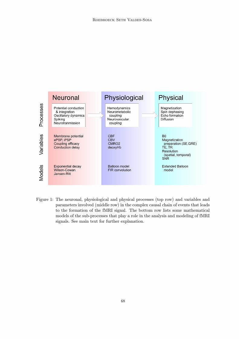
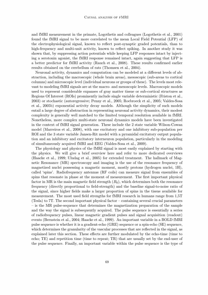
The fMRI signal reflects the activity within neuronal populations non-invasively with excel-lent spatial resolution (millimeters down to hundreds of micrometers at high field strength),good temporal resolution (seconds down to hundreds of milliseconds) and whole-brain cov-erage of the human or animal brain (Logothetis, 2008). Although fMRI is possible with afew different techniques, the Blood Oxygenation Level Dependent (BOLD) contrast mech-anism is employed in the great majority of cases. In short, the BOLD fMRI signal issensitive to changes in blood oxygenation, blood flow and blood volume that result fromoxidative glucose metabolism which, in turn, is needed to fuel local neuronal activity (Bux-ton et al., 2004). This is why fMRI is usually classified as a ‘metabolic’ or ‘hemodynamic’neuroimaging modality. Its superior spatial resolution, in particular, distinguishes it fromother functional brain imaging modalities used in humans, such as EEG, MEG and PositronEmission Tomography (PET). Although its temporal resolution is far superior to PET (an-other ‘metabolic’ neuroimaging modality) it is still an order of magnitude below that ofEEG and MEG, resulting in a relatively sparse sampling of fast neuronal processes, as wewill discuss below. The final fMRI signal arises from a complex chain of processes that wecan classify into neuronal, physiological and physical processes (Uludag et al., 2005), each ofwhich contain some crucial parameters and variables and have been modeled in various waysas illustrated in Figure 1. We will discuss each of the three classes of processes to explainthe intricacies involved in trying to model this causal chain of events with the ultimate goalof estimating neuronal activity and interactions from the measured fMRI signal.On the neuronal level, it is important to realize that fMRI reflects certain aspects of

neuronal functioning more than others. A wealth of processes are continuously in operationat the microscopic level (i.e. in any single neuron), including maintaining a resting poten-tial, post-synaptic conduction and integration (spatial and temporal) of graded excitatoryand inhibitory post synaptic potentials (EPSPs and IPSPs) arriving at the dendrites, sub-threshold dynamic (possibly oscillatory) potential changes, spike generation at the axonhillock, propagation of spikes by continuous regeneration of the action potential along theaxon, and release of neurotransmitter substances into the synaptic cleft at arrival of anaction potential at the synaptic terminal. There are many different types of neurons in themammalian brain that express these processes in different degrees and ways. In addition,there are other cells, such as glia cells, that perform important processes, some of thempossibly directly relevant to computation or signaling. As explained below, the fMRI signalis sensitive to the local oxidative metabolism in the brain. This means that, indirectly, itmainly reflects the most energy consuming of the neuronal processes. In primates, post-synaptic processes account for the great majority (about 75%) of the metabolic costs ofneuronal signaling events (Attwell and Iadecola, 2002). Indeed, the greater sensitivity offMRI to post-synaptic activity, rather than axon generation and propagation (‘spiking’),has been experimentally verified. For instance, in a simultaneous invasive electrophysiology

67


Figure 1: The neuronal, physiological and physical processes (top row) and variables andparameters involved (middle row) in the complex causal chain of events that leadsto the formation of the fMRI signal. The bottom row lists some mathematicalmodels of the sub-processes that play a role in the analysis and modeling of fMRIsignals. See main text for further explanation.

68


and fMRI measurement in the primate, Logothetis and colleagues (Logothetis et al., 2001)found the fMRI signal to be more correlated to the mean Local Field Potential (LFP) ofthe electrophysiological signal, known to reflect post-synaptic graded potentials, than tohigh-frequency and multi-unit activity, known to reflect spiking. In another study it wasshown that, by suppressing action potentials while keeping LFP responses intact by inject-ing a serotonin agonist, the fMRI response remained intact, again suggesting that LFP isa better predictor for fMRI activity (Rauch et al., 2008). These results confirmed earlierresults obtained on the cerebellum of rats (Thomsen et al., 2004).Neuronal activity, dynamics and computation can be modeled at a different levels of ab-

straction, including the macroscopic (whole brain areas), mesoscopic (sub-areas to corticalcolumns) and microscopic level (individual neurons or groups of these). The levels most rele-vant to modeling fMRI signals are at the macro- and mesoscopic levels. Macroscopic modelsused to represent considerable expanses of gray matter tissue or sub-cortical structures asRegions Of Interest (ROIs) prominently include single variable deterministic (Friston et al.,2003) or stochastic (autoregressive; Penny et al., 2005; Roebroeck et al., 2005; Valdes-Sosaet al., 2005b) exponential activity decay models. Although the simplicity of such modelsentail a large degree of abstraction in representing neuronal activity dynamics, their modestcomplexity is generally well matched to the limited temporal resolution available in fMRI.Nonetheless, more complex multi-state neuronal dynamics models have been investigatedin the context of fMRI signal generation. These include the 2 state variable Wilson-Cowanmodel (Marreiros et al., 2008), with one excitatory and one inhibitory sub-population perROI and the 3 state variable Jansen-Rit model with a pyramidal excitatory output popula-tion and an inhibitory and excitatory interneuron population, particularly in the modelingof simultaneously acquired fMRI and EEG (Valdes-Sosa et al., 2009).The physiology and physics of the fMRI signal is most easily explained by starting with

the physics. We will give a brief overview here and refer to more dedicated overviews(Haacke et al., 1999; Uludag et al., 2005) for extended treatment. The hallmark of Mag-netic Resonance (MR) spectroscopy and imaging is the use of the resonance frequency ofmagnetized nuclei possessing a magnetic moment, mostly protons (hydrogen nuclei, 1H),called ‘spins’. Radiofrequency antennas (RF coils) can measure signal from ensembles ofspins that resonate in phase at the moment of measurement. The first important physicalfactor in MR is the main magnetic field strength (B0), which determines both the resonancefrequency (directly proportional to field-strength) and the baseline signal-to-noise ratio ofthe signal, since higher fields make a larger proportion of spins in the tissue available formeasurement. The most used field strengths for fMRI research in humans range from 1,5T(Tesla) to 7T. The second important physical factor – containing several crucial parameters– is the MR pulse-sequence that determines the magnetization preparation of the sampleand the way the signal is subsequently acquired. The pulse sequence is essentially a seriesof radiofrequency pulses, linear magnetic gradient pulses and signal acquisition (readout)events (Bernstein et al., 2004; Haacke et al., 1999). An important variable in a BOLD fMRIpulse sequence is whether it is a gradient-echo (GRE) sequence or a spin-echo (SE) sequence,which determines the granularity of the vascular processes that are reflected in the signal, asexplained later this section. These effects are further modulated by the echo-time (time toecho; TE) and repetition time (time to repeat; TR) that are usually set by the end-user ofthe pulse sequence. Finally, an important variable within the pulse sequence is the type of

69


spatial encoding that is employed. Spatial encoding can primarily be achieved with gradientpulses and it embodies the essence of ‘Imaging’ in MRI. It is only with spatial encodingthat signal can be localized to certain ‘voxels’ (volume elements) in the tissue. A strengthof fMRI as a neuroimaging technique is that an adjustable trade-off is available to the userbetween spatial resolution, spatial coverage, temporal resolution and signal-to-noise ratio(SNR) of the acquired data. For instance, although fMRI can achieve excellent spatial res-olution at good SNR and reasonable temporal resolution, one can choose to sacrifice somespatial resolution to gain a better temporal resolution for any given study. Note, however,that this concerns the resolution and SNR of the data acquisition. As explained below, thephysiology of fMRI can put fundamental limitations on the nominal resolution and SNRthat is achieved in relation to the neuronal processes of interest.On the physiological level, the main variables that mediate the BOLD contrast in fMRI

are cerebral blood flow (CBF), cerebral blood volume (CBV) and the cerebral metabolicrate of oxygen (CMRO2) which all change the oxygen saturation of the blood (as usefullyquantified by the concentration of deoxygenated hemoglobin). The BOLD contrast is madepossible by the fact that oxygenation of the blood changes its magnetic susceptibility, whichhas an effect on the MR signal as measured in GRE and SE sequences. More precisely,oxygenated and deoxygenated hemoglobin (oxy-Hb and deoxy-Hb) have different magneticproperties, the former being diamagnetic and the latter paramagnetic. As a consequence,deoxygenated blood creates local microscopic magnetic field gradients, such that local spinensembles dephase, which is reflected in a lower MR signal. Conversely oxygenation of bloodabove baseline lowers the concentration of deoxy-Hb, which decreases local spin dephasingand results in a higher MR signal. This means that fMRI is directly sensitive to the relativeamount of oxy- and deoxy Hb and to the fraction of cerebral tissue that is occupied by blood(the CBV), which are controlled by local neurovascular coupling processes. Neurovascularprocesses, in turn, are tightly coupled to neurometabolic processes controlling the rate ofoxidative glucose metabolism (the CMRO2) that is needed to fuel neural activity.Naively one might expect local neuronal activity to quickly increase CMRO2 and increase

the local concentration of deoxy-Hb, leading to a lowering of the MR signal. However, thistransient increase in deoxy-Hb or the initial dip in the fMRI signal is not consistentlyobserved and, thus, there is a debate whether this signal is robust, elusive or simply notexistent (Buxton, 2001; Ugurbil et al., 2003; Uludag, 2010). Instead, early experimentsshowed that the dynamics of blood flow and blood volume, the hemodynamics, lead to arobust BOLD signal increase. Neuronal activity is quickly followed by a large CBF increasethat serves the continued functioning of neurons by clearing metabolic by-products (suchas CO2) and supplying glucose and oxy-Hb. This CBF response is an overcompensatingresponse, supplying much more oxy-Hb to the local blood system than has been metabolized.As a consequence, within 1-2 seconds, the oxygenation of the blood increases and theMR signal increases. The increased flow also induces a ‘ballooning’ of the blood vessels,increasing CBV, the proportion of volume taken up by blood, further increasing the signal.A mathematical characterization of the hemodynamic processes in BOLD fMRI at 1.5-3T

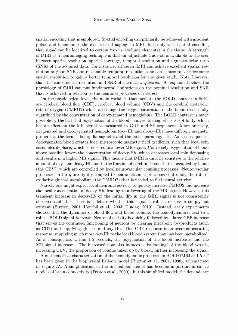
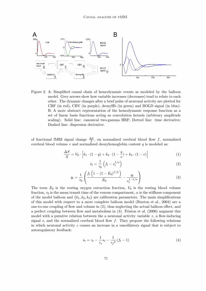
has been given in the biophysical balloon model (Buxton et al., 2004, 1998), schematizedin Figure 2A. A simplification of the full balloon model has become important in causalmodels of brain connectivity (Friston et al., 2000). In this simplified model, the dependence

70


Figure 2: A: Simplified causal chain of hemodynamic events as modeled by the balloonmodel. Grey arrows show how variable increases (decreases) tend to relate to eachother. The dynamic changes after a brief pulse of neuronal activity are plotted forCBF (in red), CBV (in purple), deoxyHb (in green) and BOLD signal (in blue).B: A more abstract representation of the hemodynamic response function as aset of linear basis functions acting as convolution kernels (arbitrary amplitudescaling). Solid line: canonical two-gamma HRF; Dotted line: time derivative;Dashed line: dispersion derivative.

of fractional fMRI signal change ΔSS , on normalized cerebral blood flow f , normalizedcerebral blood volume v and normalized deoxyhemoglobin content q is modeled as:

ΔS

S= V0 ∙

[k1 ∙ (1− q) + k2 ∙ (1−

q

v) + k3 ∙ (1− v)

](1)

vt =1

τ0

(ft − v

1/αt

)(2)

qt =1

τ0

ft

(1− (1− E0)

1/ft)

E0−

qt

v1−1/αt

(3)

The term E0 is the resting oxygen extraction fraction, V0 is the resting blood volumefraction, τ0 is the mean transit time of the venous compartment, α is the stiffness componentof the model balloon and {k1, k2, k3} are calibration parameters. The main simplificationsof this model with respect to a more complete balloon model (Buxton et al., 2004) are aone-to-one coupling of flow and volume in (2), thus neglecting the actual balloon effect, anda perfect coupling between flow and metabolism in (3). Friston et al. (2000) augment thismodel with a putative relation between the a neuronal activity variable z, a flow-inducingsignal s, and the normalized cerebral blood flow f . They propose the following relationsin which neuronal activity z causes an increase in a vasodilatory signal that is subject toautoregulatory feedback:

st = zt −1

τsst −

1

τf 2(ft − 1) (4)

71


ft = st (5)

Here τs is the signal decay time constant, τf is the time-constant of the feedback autoregula-tory mechanism1, and f is the flow normalized to baseline flow. The physiological interpre-tation of the autoregulatory mechanism is unspecified, leaving us with a neuronal activityvariable z that is measured in units of s−2. The physiology of the hemodynamics containedin differential equations (2) to (5), on the other hand, is more readily interpretable, andwhen integrated for a brief neuronal input pulse shows the behavior as described above(Figure 2A, upper panel). This simulation highlights a few crucial features. First, thehemodynamic response to a brief neural activity event is sluggish and delayed, entailingthat the fMRI BOLD signal is a delayed and low-pass filtered version of underlying neu-ronal activity. More than the distorting effects of hemodynamic processes on the temporalstructure of fMRI signals per se, it is the difference in hemodynamics in different parts ofthe brain that forms a severe confound for dynamic brain connectivity models. Particu-larly, the delay imposed upon fMRI signals with respect to the underlying neural activityis known to vary between subjects and between different brain regions of the same sub-ject (Aguirre et al., 1998; Saad et al., 2001). Second, although CBF, CBV and deoxyHbchanges range in the tens of percents, the BOLD signal change at 1.5T or 3T is in the rangeof 0.5-2%. Nevertheless, the SNR of BOLD fMRI in general is very good in comparison toelectrophysiological techniques like EEG and MEG.Although the balloon model and its variations have played an important role in describing

the transient features of the fMRI response and inferring neuronal activity, simplified waysof representing the BOLD signal responses are very often used. Most prominent amongthese is a linear finite impulse response (FIR) convolution with a suitable kernel. Themost used single convolution kernel characterizing the ‘canonical’ hemodynamic reponse isformed by a superposition of two gamma functions (Glover, 1999), the first characterizingthe initial signal increase, the second the later negative undershoot (Figure 2B, solid line):

h (t) = m1tτ1e(−l1t) − cm2tτ2e(−l2t)

mi = max(tτie(−lit)

) (6)

With times-to-peak in seconds τ1 = 6, τ2 = 16, scale parameters li (typically equal to 1)and a relative amplitude of undershoot to peak of c = 1/6.Often, the canonical two-gamma HRF kernel is augmented with one or two additional

orthogonalized convolution kernels: a temporal derivative and a dispersion derivative. To-gether the convolution kernels form a flexible basis function expansion of possible HRFshapes, with the temporal derivative of the canonical accounting for variation in the re-sponse delay and the dispersion derivative accounting for variations in temporal responsewidth (Henson et al., 2002; Liao et al., 2002). Thus, the linear basis function representationis a more abstract characterization of the HRF (i.e. further away from the physiology) thatstill captures the possible variations in responses.It is an interesting property of hemodynamic processes that, although they are charac-

terized by a large overcompensating reaction to neuronal activity, their effects are highly

1. Note that we have reparametrized the equation here in terms of τf2 to make τf a proper time constant

in units of seconds

72


local. The locality of the hemodynamic reponse to neuronal activity limits the actual spa-tial resolution of fMRI. The path blood inflow in the brain is from large arteries througharterioles into capillaries where exchange with neuronal tissue takes place at a microscopiclevel. Blood outflow takes place via venules into the larger veins. The main regulators ofblood flow are the arterioles that are surrounded by smooth muscle, although arteries andcapillaries are also thought to be involved in blood flow regulation (Attwell et al., 2010).Different hemodynamic parameters have different spatial resolutions. While CBV and CBFchanges in all compartments but mostly venules, oxygenation changes mostly in the venulesand veins. Thus, the achievable spatial resolution with fMRI is limited by its specificity tothe smaller arterioles and venules and microscopic capillaries supplying the tissue, ratherthan the larger supplying arteries draining veins. The larger vessels have a larger domainof supply or extraction and, as a consequence, their signal is blurred and mislocalized withrespect to active tissue. Here, physiology and physics interact in an important way. It canbe shown theoretically – by the effects of thermal motion of spin diffusion over time andthe distance of the spins to deoxy-Hb – that the origin of the BOLD signal in SE sequencesat high main field strengths (larger than 3T) is much more specific to the microscopic vas-culature than to the larger arteries and veins. This does not hold for GRE sequences orSE sequences at lower field strengths. The cost of this greater specificity and higher effec-tive spatial resolution is that SE-BOLD has a lower intrinsic SNR than GRE-BOLD. Theballoon model equations above are specific to GRE-BOLD at 1.5T and 3T and have beenextended to reflect diffusion effects for higher field strengths (Uludag et al., 2009).In summary, fMRI is an indirect measure of neuronal and synaptic activity. The phys-

iological quantities directly determining signal contrast in BOLD fMRI are hemodynamicquantities such as cerebral blood flow and volume and oxygen metabolism. fMRI can achievea excellent spatial resolution (millimeters down to hundreds of micrometers at high fieldstrength) with good temporal resolution (seconds down to hundreds of milliseconds). Thepotential to resolve neuronal population interactions at a high spatial resolution is whatdrives attempts at causal time series modeling of fMRI data. However, the significant as-pects of fMRI that pose challenges for such attempts are i) the enormous dimensionality ofthe data that contains hundreds of thousands of channels (voxels) ii) the temporal convo-lution of neuronal events by sluggish hemodynamics that can differ between remote partsof the brain and iii) the relatively sparse temporal sampling of the signal.

3. Causality and state-space models

The inference of causal influence relations from statistical analysis of observed data has twodominant approaches. The first approach is in the tradition of Granger causality or G-causality, which has its signature in improved predictability of one time series by another.The second approach is based on graphical models and the notion of intervention (Glymour,2003), which has been formalized using a Bayesian probabilistic framework termed causalcalculus or do-calculus (Pearl, 2009). Interestingly, recent work has combined of the twoapproaches in a third line of work, termed Dynamic Structural Systems (White and Lu,2010). The focus here will be on the first approach, initially firmly rooted in econometricsand time-series analysis. We will discuss this tradition in a very general form, acknowledging

73


early contributions fromWiener, Akaike, Granger and Schweder and will follow (Valdes-Sosaet al., in press) in refering to the crucial concept as WAGS influence.

3.1. Wiener-Akaike-Granger-Schweder (WAGS) influence

The crucial premise of the WAGS statistical causal modeling tradition is that a cause mustprecede and increase the predictability of its effect. In other words: a variable X2 influencesanother variable X1 if the prediction of X1 improves when we use past values of X2, giventhat all other relevant information (importantly: the past of X1 itself) is taken into account.This type of reasoning can be traced back at least to Hume and is particularly popular inanalyzing dynamical data measured as time series. In a formal framework it was originallyproposed (in an abstract form) byWiener (Wiener, 1956), and then introduced into practicaldata analysis and popularized by Granger (Granger, 1969). A point stressed by Granger isthat increased predictability is a necessary but not sufficient condition for a causal relationbetween time series. In fact, Granger distinguished true causal relations – only to be inferredin the presence of knowledge of the state of the whole universe – from “prima facie” causalrelations that we refer to as “influence” in agreement with other authors (Commenges andGegout-Petit, 2009). Almost simultaneous with Grangers work, Akaike (Akaike, 1968), andSchweder (Schweder, 1970) introduced similar concepts of influence, prompting (Valdes-Sosaet al., in press) to coin the term WAGS influence (for Wiener-Akaike-Granger-Schweder).This is a generalization of a proposal by placeAalen (Aalen, 1987; Aalen and Frigessi, 2007)who was among the first to point out the connections between Granger’s and Schweder’sinfluence concepts. Within this framework we can define several general types of WAGSinfluence, which are applicable to both Markovian and non-Markovian processes, in discreteor continuous time.For three vector time series X1 (t) , X2 (t) , X3 (t) we wish to know if time series X1 (t) isinfluenced by time series X2 (t) conditional on X3 (t). Here X3 (t) can be considered anyset of relevant time series to be controlled for. Let X [a, b] = {X (t) , t ∈ [a, b]} denote thehistory of a time series in the discrete or continuous time interval [a, b] The first categoricaldistinction is based on what part of the present or future of X1 (t) can be predicted by thepast or present of X2 (τ2) τ2 ≤ t. This leads to the following classification (Florens, 2003;Florens and Fougere, 1996):

1. If X2 (τ2) : τ2 < t , can influence any future value of X1 (t) it is a global influence.

2. If X2 (τ2) : τ2 < t , can influence X1 (t) at time t it is a local influence.

3. If X2 (τ2) : τ2 = t , can influence X1 (t) it is a contemporaneous influence.

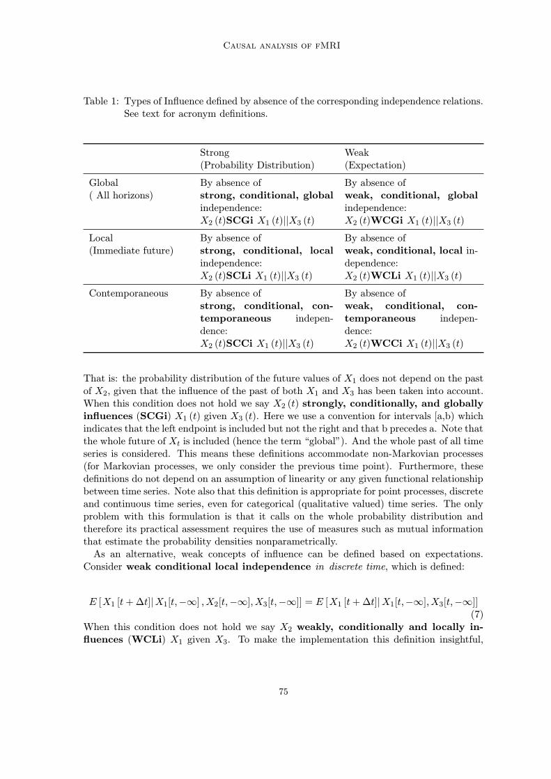
A second distinction is based on predicting the whole probability distribution (stronginfluence) or only given moments (weak influence). Since the most natural formal definitionis one of independence, every influence type amounts to the negation of an independencestatement. The two classifications give rise to six types of independence and correspondinginfluence as set out in Table 1.To illustrate, X1 (t) is strongly, conditionally, and globally independent of X2 (t)given X3 (t), if

P (X1(∞, t]|X1(t,−∞], X2(t,−∞], X3(t,−∞]) = P (X1(∞, t]|X1(t,−∞], X3(t,−∞])

74


Table 1: Types of Influence defined by absence of the corresponding independence relations.See text for acronym definitions.

Strong(Probability Distribution)

Weak(Expectation)

Global( All horizons)

By absence ofstrong, conditional, globalindependence:X2 (t)SCGi X1 (t)||X3 (t)

By absence ofweak, conditional, globalindependence:X2 (t)WCGi X1 (t)||X3 (t)

Local(Immediate future)

By absence ofstrong, conditional, localindependence:X2 (t)SCLi X1 (t)||X3 (t)

By absence ofweak, conditional, local in-dependence:X2 (t)WCLi X1 (t)||X3 (t)

Contemporaneous By absence ofstrong, conditional, con-temporaneous indepen-dence:X2 (t)SCCi X1 (t)||X3 (t)

By absence ofweak, conditional, con-temporaneous indepen-dence:X2 (t)WCCi X1 (t)||X3 (t)

That is: the probability distribution of the future values of X1 does not depend on the pastof X2, given that the influence of the past of both X1 and X3 has been taken into account.When this condition does not hold we say X2 (t) strongly, conditionally, and globallyinfluences (SCGi) X1 (t) given X3 (t). Here we use a convention for intervals [a,b) whichindicates that the left endpoint is included but not the right and that b precedes a. Note thatthe whole future of Xt is included (hence the term “global”). And the whole past of all timeseries is considered. This means these definitions accommodate non-Markovian processes(for Markovian processes, we only consider the previous time point). Furthermore, thesedefinitions do not depend on an assumption of linearity or any given functional relationshipbetween time series. Note also that this definition is appropriate for point processes, discreteand continuous time series, even for categorical (qualitative valued) time series. The onlyproblem with this formulation is that it calls on the whole probability distribution andtherefore its practical assessment requires the use of measures such as mutual informationthat estimate the probability densities nonparametrically.As an alternative, weak concepts of influence can be defined based on expectations.

Consider weak conditional local independence in discrete time, which is defined:

E [X1 [t+Δt]|X1[t,−∞] , X2[t,−∞], X3[t,−∞]] = E [X1 [t+Δt]|X1[t,−∞], X3[t,−∞]](7)

When this condition does not hold we say X2 weakly, conditionally and locally in-fluences (WCLi) X1 given X3. To make the implementation this definition insightful,

75


consider a discrete first-order vector auto-regressive (VAR) model for X = [X1X2X3]:

X [t+Δt] = AX [t] + e [t+Δt] (8)

For this case E [X[t+Δt]|X[t,−∞]] = AX [t], and analyzing influence reduces to findingwhich of the autoregressive coefficients are zero. Thus, many proposed operational tests ofWAGS influence, particularly in fMRI analysis, have been formulated as tests of discreteautoregressive coefficients, although not always of order 1. Within the same model one canoperationalize weak conditional instantaneous independence in discrete time as zerooff-diagonal entries in the co-variance matrix of the innovations e[t]:

Σe = cov [X [t+Δt] |X [t,−∞]] = E[X [t+Δt]X ′ [t+Δt] |X [t,−∞]

]

In comparison weak conditional local independence in continuous time is defined:

E [Y1[t]|Y1(t,−∞], Y2(t,−∞], Y3(t,−∞]] = E [Y1[t]|Y1(t,−∞], Y3(t,−∞]] (9)

Now consider a first-order stochastic differential equation (SDE) model for Y = [Y1Y2Y3]:

dY = BY dt+ dω (10)

Then, since ω is a Wiener process with zero-mean white Gaussian noise as a derivative,E [Y [t]|Y (t,−∞]] = B Y (t)and analysing influence amounts to estimating the parametersB of the SDE. However, if one were to observe a discretely sampled versionX[k] = Y (kΔt)at sampling interval Δtand model this with the discrete autoregressive model above, thiswould be inadequate to estimate the SDE parameters for large Δt, since the exact relationsbetween continuous and discrete system matrices are known to be:

A = eBΔt = I+∞∑

i=1

Δti

i! Bi

Σe =∫ t+Δtt eBs

∑ω eBsds

(11)

The power series expansion of the matrix exponential in the first line shows A to be aweighted sum of successive matrix powers Biof the continuous time system matrix. Thus,the Awill contain contributions from direct (in B) and indirect (in i steps inBi) causal linksbetween the modeled areas. The contribution of the more indirect links is progressivelydown-weighted with the number of causal steps from one area to another and is smallerwhen the sampling interval Δt is smaller. This makes clear that multivariate discretesignal models have some undesirable properties for coarsely sampled signals (i.e. a largeΔt with respect to the system dynamics), such as fMRI data. Critically, entirely rulingout indirect influences is not actually achieved merely by employing a multivariate discretemodel. Furthermore, estimated WAGS influence (particularly the relative contribution ofindirect links) is dependent on the employed sampling interval. However, the discrete systemmatrix still represents the presence and direction of influence, possibly mediated throughother regions.When the goal is to estimate WAGS influence for discrete data starting from a continuous

time model, one has to model explicitly the mapping to discrete time. Mapping continu-ous time predictions to discrete samples is a well known topic in engineering and can be

76


solved by explicit integration over discrete time steps as performed in (11) above. Althoughthis defines the mapping from continuous to discrete parameters, it does not solve the re-verse assignment of estimating continuous model parameters from discrete data. Doing sorequires a solution to the aliasing problem (Mccrorie, 2003) in continuous stochastic sys-tem identification by setting sufficient conditions on the matrix logarithm function to makeBabove identifiable (uniquely defined) in terms of A. Interesting in this regard is a lineof work initiated by Bergstrom (Bergstrom, 1966, 1984) and Phillips (Phillips, 1973, 1974)studying the estimation of continuous time Autoregressive models (McCrorie, 2002), andcontinuous time Autoregressive Moving Average Models (Chambers and Thornton, 2009)from discrete data. This work rests on the observation that the lag zero covariance matrixΣewill show contemporaneous covariance even if the continuous covariance matrix Σω isdiagonal. In other words, the discrete noise becomes correlated over the discrete time-seriesbecause the random fluctuations are aggregated over time. Rather than considering this adisadvantage, this approach tries to use both lag information (the AR part) and zero-lagcovariance information to identify the underlying continuous linear model.Notwithstanding the desirability of a continuous time model for consistent inference on

WAGS influence, there are a few invariances of discrete VAR models, or more generallydiscrete Vector Autoregressive Moving Average (VARMA) models that allow their carefullyqualified usage in estimating causal influence. The VAR formulation of WAGS influencehas the property of invariance under invertible linear filtering. More precisely, a generalmeasure of influence remains unchanged if channels are each pre-multiplied with differentinvertible lag operators (Geweke, 1982). However, in practice the order of the estimatedVAR model would need to be sufficient to accommodate these operators. Beyond invert-ible linear filtering, a VARMA formulation has further invariances. Solo (2006) showedthat causality in a VARMA model is preserved under sampling and additive noise. Moreprecisely, if both local and contemporaneous influence is considered (as defined above) theVARMA measure is preserved under sampling and under the addition of independent butcolored noise to the different channels. Finally, Amendola et al. (2010) shows the class ofVARMA models to be closed under aggregation operations, which include both samplingand time-window averaging.

3.2. State-space models

A general state-space model for a continuous vector time-series y (t)can be formulated withthe set of equations:

x (t) = f (x (t) , v (t) ,Θ) + ω (t)y (t) = g (x (t) , v (t) ,Θ) + ε (t)

(12)

This expresses the observed time-series y (t)as a function of the state variables x (t), whichare possibly hidden (i.e. unobserved) and observed exogenous inputs v (t), which are pos-sibly under control. All parameters in the model are grouped into Θ. Note that somegenerality is sacrificed from the start since fand gdo not depend on t (The model is au-tonomous and generates stationary processes) or on ω (t) or ε (t), that is: noise enters onlyadditively. The first set of equations, the transition equations or state equations, describethe evolution of the dynamic system over time in terms of stochastic differential equations

77


(SDEs, though technically only when ω (t) = Σw (t) with w (t) a Wiener process), capturingrelations among the hidden state variables x (t) themselves and the influence of exogenousinputs v (t). The second set of equations, the observation equations or measurement equa-tions, describe how the measurement variables y (t) are obtained from the instantaneousvalues of the hidden state variables x (t) and the inputs v (t). In fMRI experiments theexogenous inputs v (t) mostly reflect experimental control and often have the form of a sim-ple indicator function that can represent, for instance, the presence or absence of a visualstimulus. The vector-functions fand g can generally be non-linear.The state-space formalism allows representation of a very large class of stochastic pro-

cesses. Specifically, it allows representation of both so-called ‘black-box ’ models, in whichparameters are treated as means to adjust the fit to the data without reflecting physicallymeaningful quantities, and ‘grey-box ’ models, in which the adjustable parameters do havea physical or physiological (in the case of the brain) interpretation. A prominent exampleof a black-box model in econometric time-series analysis and systems identification is the(discrete) Vector Autoregressive Moving Average model with exogenous inputs (VARMAXmodel) defined as (Ljung, 1999; Reinsel, 1997):

F (B) yt = G (B) vt + L (B) et ⇔∑pi=0 Fiyt−i =

∑sj=0Gjvt−j +

∑qk=0 Lket−k

(13)

Here, the backshift operator B is defined, for any ηt as Biηt = ηt−i and F , G and L are

polynomials in the backshift operator, such that e.g. F (B) =∑pi=0 FiB

i and p, s and q arethe dynamic orders of the VARMAX(p,s,q) model. The minimal constraints on (13) to makeit identifiable are F0 = L0 = I, which yields the standard VARMAX representation. TheVARMAX model and its various reductions (by use of only one or two of the polynomials,e.g. VAR, VARX or VARMA models) have played a large role in time-series prediction andWAGS influence modeling. Thus, in the context of state space models it is important toconsider that the VARMAX model form can be equivalently formulated in a discrete linearstate space form:

xk+1 = Axk +Bvk +Kekyk = Cxk +Dvk + ek

(14)

In turn the discrete linear state space form can be explicitly accommodated by the contin-uous general state-space framework in (12) when we define:

f (x (t) , v (t) ,Θ) ' Fx (t) +Gv (t)g (x (t) , v (t) ,Θ) ' Hx (t) +Dv (t)

ω (t) = Kε (t)

Θ ={F,G,H,D, K,Σe

} (15)

Again, the exact relations between the discrete and continuous state space parameter ma-trices can be derived analytically by explicit integration over time (Ljung, 1999). And, asdiscussed above, wherever discrete data is used to model continuous influence relations theproblems of temporal aggregation and aliasing have to be taken into account.Although analytic solutions for the discretely sampled continuous linear systems exist, the

discretization of the nonlinear stochastic model (12) does not have a unique global solution.However, physiological models of neuronal population dynamics and hemodynamics areformulated in continuous time and are mostly nonlinear while fMRI data is inherently

78


discrete with low sampling frequencies. Therefore, it is the discretization of the nonlineardynamical stochastic models that is especially relevant to causal analysis of fMRI data.A local linearization approach was proposed by (Ozaki, 1992) as bridge between discretetime series models and nonlinear continuous dynamical systems model. Considering thenonlinear state equation without exogenous input:

x (t) = f (x (t)) + ω (t) . (16)

The essential assumption in local linearization (LL) of this nonlinear system is to consider

the Jacobian matrix J (l,m) = ∂fl(X)∂Xm

as constant over the time period [t+Δt, t]. ThisJacobian plays the same role as the autoregressive matrix in the linear systems above.Integration over this interval gives the solution:

xk+1 = xk + J−1(eJΔt − I) f (xk) + ek+1 (17)

where I is the identity matrix. Note integration should not be computed this way sinceit is numerically unstable, especially when the Jacobian is poorly conditioned. A list ofrobust and fast procedures is reviewed in (Valdes-Sosa et al., 2009). This solution is locallylinear but crucially it changes with the state at the beginning of each integration interval;this is how it accommodates nonlinearity (i.e., a state-dependent autoregression matrix).As above, the discretized noise shows instantaneous correlations due to the aggregation ofongoing dynamics within the span of a sampling period. Once again, this highlights theunderlying mechanism for problems with temporal sub-sampling and aggregation for somediscrete time models of WAGS influence.

4. Dynamic causality in fMRI connectivity analysis

Two streams of developments have recently emerged that make use of the temporal dy-namics in the fMRI signal to analyse directed influence (effective connectivity): Grangercausality analysis (GCA; Goebel et al., 2003; Roebroeck et al., 2005; Valdes-Sosa, 2004) inthe tradition of time series analysis and WAGS influence on the one hand, and DynamicCausal Modeling (DCM; Friston et al., 2003) in the tradition of system control on the otherhand. As we will discuss in the final section, these approaches have recently started devel-oping into an integrated single direction. However, initially each was focused on separateissues that pose challenges for the estimation of causal influence from fMRI data. WhereasDCM is formulated as an explicit grey box state space model to account for the temporalconvolution of neuronal events by sluggish hemodynamics, GCA analysis has been mostlyaimed at solving the problem of region selection in the enormous dimensionality of fMRIdata.

4.1. Hemodynamic deconvolution in a state space approach

While having a long history in engineering, state space modeling was only introduced re-cently for the inference of neural states from neuroimaging signals. The earliest attemptstargeted estimating hidden neuronal population dynamics from scalp-level EEG data (Her-nandez et al., 1996; Valdes-Sosa et al., 1999). This work first advanced the idea that state

79


space models and appropriate filtering algorithms are an important tool to estimate thetrajectories of hidden neuronal processes from observed neuroimaging data if one can for-mulate an accurate model of the processes leading from neuronal activity to data records.A few years later, this idea was robustly transferred to fMRI data in the form of DCM(Friston et al., 2003). DCM combines three ideas about causal influence analysis in fMRIdata (or neuroimaging data in general), which can be understood in terms of the discussionof the fMRI signal and state space models above (Daunizeau et al., 2009a).First, neuronal interactions are best modeled at the level of unobserved (latent) signals,

instead of at the level of observed BOLD signals. This requires a state space model with adynamic model of neuronal population dynamics and interactions. The original model thatwas formulated for the dynamics of neuronal states x = {x1, . . . , xN} is a bilinear ODEmodel:

x = Ax+∑vjB

jx+Cv (18)

That is, the noiseless neuronal dynamics are characterized by a linear term (with entries inA representing intrinsic coupling between populations), an exogenous term (with C repre-senting driving influence of experimental variables) and a bilinear term (with Bj represent-ing the modulatory influence of experimental variables on coupling between populations).More recent work has extended this model, e.g. by adding a quadratic term (Stephan et al.,2008), stochastic dynamics (Daunizeau et al., 2009b) or multiple state variables per region(Marreiros et al., 2008).Second, the latent neuronal dynamics are related to observed data by a generative (for-

ward) model that accounts for the temporal convolution of neuronal events by slow andvariably delayed hemodynamics. This generative forward model in DCM for fMRI is ex-actly the (simplified) balloon model set out in section 2. Thus, for every selected regiona single state variable represents the neuronal or synaptic activity of a local population ofneurons and (in DCM for BOLD fMRI) four or five more represent hemodynamic quanti-ties such as capillary blood volume, blood flow and deoxy-hemoglobin content. All statevariables (and the equations governing their dynamics) that serve the mapping of neuronalactivity to the fMRI measurements (including the observation equation) can be called theobservation model. Most of the physiologically motivated generative model in DCM forfMRI is therefore concerned with an observation model encapsulating hemodynamics. Theparameters in this model are estimated conjointly with the parameters quantifying neuronalconnectivity. Thus, the forward biophysical model of hemodynamics is ‘inverted’ in the es-timation procedure to achieve a deconvolution of fMRI time series and obtain estimates ofthe underlying neuronal states. DCM has also been applied to EEG/MEG, in which casethe observation model encapsulates the lead-field matrix from neuronal sources to EEGelectrodes or MEG sensors (Kiebel et al., 2009).Third, the approach to estimating the hidden state trajectories (i.e. filtering and smooth-

ing) and parameter values in DCM is cast in a Bayesian framework. In short, Bayes’ theoremis used to combine priors p(Θ|M)and likelihood p (y|Θ,M)into the marginal likelihood orevidence:

p (y|M) =∫p (y|Θ,M) p (Θ|M) dΘ (19)

80


Here, the modelM is understood to define the priors on all parameters and the likelihoodthrough the generative models for neuronal dynamics and hemodynamics. A posteriorfor the parameters p (Θ|y,M) can be obtained as the distribution over parameters whichmaximizes the evidence (19). Since this optimization problem has no analytic solutionand is intractable with numerical sampling schemes for complex models, such as DCM,approximations must be used. The inference approach for DCM relies on variational Bayesmethods (Beal, 2003) that optimize an approximation density q(Θ) to the posterior. Theapproximation density is taken to have a Gaussian form, which is often referred to as the“Laplace approximation” (Friston et al., 2007). In addition to the approximate posterior onthe parameters, the variational inference will also result into a lower bound on the evidence,sometimes referred to as the “free energy”. This lower bound (or other approximationsto the evidence, such as the Akaike Information Criterion or the Bayesian InformationCriterion) are used for model comparison (Penny et al., 2004). Importantly, these quantitiesexplicitly balance goodness-of-it against model complexity as a means of avoiding overfitting.An important limiting aspect of DCM for fMRI is that the models M that are compared

also (implicitly) contain an anatomical model or structural model that contains i) a selectionof the ROIs in the brain that are assumed to be of importance in the cognitive process ortask under investigation, ii) the possible interactions between those structures and iii) thepossible effects of exogenous inputs onto the network. In other words, each model Mspecifies the nodes and edges in a directed (possibly cyclic) structural graph model. Sincethe anatomical model also determines the selected part y of the total dataset (all voxels)one cannot use the evidence to compare different anatomical models. This is because theevidence of different anatomical models is defined over different data. Applications of DCMto date invariably use very simple anatomical models (typically employing 3-6 ROIs) incombination with its complex parameter-rich dynamical model discussed above. The cleardanger with overly simple anatomical models is that of spurious influence: an erroneousinfluence found between two selected regions that in reality is due to interactions withadditional regions which have been ignored. Prototypical examples of spurious influence,of relevance in brain connectivity, are those between unconnected structures A and B thatreceive common input from, or are intervened by, an unmodeled region C.

4.2. Exploratory approaches for model selection

Early applications of WAGS influence to fMRI data were aimed at counteracting the prob-lems with overly restrictive anatomical models by employing more permissive anatomicalmodels in combination with a simple dynamical model (Goebel et al., 2003; Roebroecket al., 2005; Valdes-Sosa, 2004). These applications reflect the observation that estimationof mathematical models from time-series data generally has two important aspects: modelselection and model identification (Ljung, 1999). In the model selection stage a class ofmodels is chosen by the researcher that is deemed suitable for the problem at hand. In themodel identification stage the parameters in the chosen model class are estimated from theobserved data record. In practice, model selection and identification often occur in a some-what interactive fashion where, for instance, model selection can be informed by the fit ofdifferent models to the data achieved in an identification step. The important point is thatmodel selection involves a mixture of choices and assumptions on the part of the researcher

81


and the information gained from the data-record itself. These considerations indicate thatan important distinction must be made between exploratory and confirmatory approaches,especially in structural model selection procedures for brain connectivity. Exploratory tech-niques use information in the data to investigate the relative applicability of many models.As such, they have the potential to detect ‘missing’ regions in structural models. Confirma-tory approaches, such as DCM, test hypotheses about connectivity within a set of modelsassumed to be applicable. Sources of common input or intervening causes are taken intoaccount in a multivariate confirmatory model, but only if the employed structural modelallows it (i.e. if the common input or intervening node is incorporated in the model).The technique of Granger Causality Mapping (GCM) was developed to explore all re-

gions in the brain that interact with a single selected reference region using autoregressivemodeling of fMRI time-series (Roebroeck et al., 2005). By employing a simple bivariatemodel containing the reference region and, in turn, every other voxel in the brain, thesources and targets of influence for the reference region can be mapped. It was shown thatsuch an ‘exploratory’ mapping approach can form an important tool in structural modelselection. Although a bivariate model does not discern direct from indirect influences, themapping approach locates potential sources of common input and areas that could act asintervening network nodes. In addition, by settling for a bivariate model one trivially avoidsthe conflation of direct and indirect influences that can arise in discrete AR model due totemporal aggregation, as discussed above. Other applications of autoregressive modeling tofMRI data have considered full multivariate models on large sets of selected brain regions,illustrating the possibility to estimate high-dimensional dynamical models. For instance,Valdes-Sosa (2004) and Valdes-Sosa et al. (2005b) applied these models to parcellations ofthe entire cortex in conjunction with sparse regression approaches that enforce an implicitstructural model selection within the set of parcels. In another more recent example (Desh-pande et al., 2008) a full multivariate model was estimated over 25 ROIs (that were found tobe activated in the investigated task) together with an explicit reduction procedure to pruneregions from the full model as a structural model selection procedure. Additional variantsof VAR model based causal inference that has been applied to fMRI include time vary-ing influence (Havlicek et al., 2010), blockwise (or ‘cluster-wise’) influence from one groupof variables to another (Barrett et al., 2010; Sato et al., 2010) and frequency-decomposedinfluence (Sato et al., 2009).The initial developments in autoregressive modeling of fMRI data led to a number of

interesting applications studying human mental states and cognitive processes, such asgestural communication (Schippers et al., 2010), top-down control of visual spatial atten-tion (Bressler et al., 2008), switching between executive control and default-mode networks(Sridharan et al., 2008), fatigue (Deshpande et al., 2009) and the resting state (Uddinet al., 2009). Nonetheless, the lack of AR models to account for the varying hemodynamicsconvolving the signals of interest and aggregation of dynamics between time samples hasprompted a set of validation studies evaluating the conditions under which discrete ARmodels can provide reliable connectivity estimates. In (Roebroeck et al., 2005) simulationswere performed to validate the use of bivariate AR models in the face of hemodynamic con-volution and sampling. They showed that under these conditions (even without variabilityin hemodynamics) AR estimates for a unidirectional influence are biased towards inferringbidirectional causality, a well known problem when dealing with aggregated time series

82


(Wei, 1990). They then went on to show that instead unbiased non-parametric inferencefor bivariate AR models can be based on a difference of influence terms (X → Y −Y → X).In addition, they posited that inference on such influence estimates should always includeexperimental modulation of influence, in order to rule out hemodynamic variation as anunderlying reason for spurious causality. In Deshpande et al. (2010) the authors simulatedfMRI data by manipulating the causal influence and neuronal delays between local fieldpotentials (LFPs) acquired from the macaque cortex and varying the hemodynamic delaysof a convolving hemodynamic response function and the signal-to-noise ratio (SNR) andthe sampling period of the final simulated fMRI data. They found that in multivariate(4 dimensional) simulations with hemodynamic and neuronal delays drawn from a uniformrandom distribution correct network detection from fMRI was well above chance and wasup to 90% under conditions of fast sampling and low measurement noise. Other studiesconfirmed the observation that techniques with intermediate temporal resolution, such asfMRI, can yield good estimates of the causal connections based on AR models (Stevensonand Kording, 2010), even in the face of variable hemodynamics (Ryali et al., 2010). However,another recent simulation study, investigating a host of connectivity methods concluded lowdetection performance of directed influence by AR models under general conditions (Smithet al., 2010).

4.3. Toward integrated models

David et al. (2008) aimed at direct comparison of autoregressive modeling and DCM forfMRI time series and explicitly pointed at deconvolution of variable hemodynamics forcausality inferences. The authors created a controlled animal experiment where gold stan-dard validation of neuronal connectivity estimation was provided by intracranial EEG(iEEG) measurements. As discussed extensively in Friston (2009b) and Roebroeck et al.(2009a) such a validation experiment can provide important information on best practicesin fMRI based brain connectivity modeling that, however, need to be carefully discussedand weighed. In David et al.’s study, simultaneous fMRI, EEG, and iEEG were measured in6 rats during epileptic episodes in which spike-and-wave discharges (SWDs) spread throughthe brain. fMRI was used to map the hemodynamic response throughout the brain to seizureactivity, where ictal and interictal states were quantified by the simultaneously recordedEEG. Three structures were selected by the authors as the crucial nodes in the networkthat generates and sustains seizure activity and further analysed with i) DCM, ii) simple ARmodeling of the fMRI signal and iii) AR modeling applied to neuronal state-variable esti-mates obtained with a hemodynamic deconvolution step. By applying G-causality analysisto deconvolved fMRI time-series, the stochastic dynamics of the linear state-space model areaugmented with the complex biophysically motivated observation model in DCM. This stepis crucial if the goal is to compare the dynamic connectivity models and draw conclusions onthe relative merits of linear stochastic models (explicitly estimating WAGS influence) andbilinear deterministic models. The results showed both AR analysis after deconvolution andDCM analysis to be in accordance with the gold-standard iEEG analyses, identifying themost pertinent influence relations undisturbed by variations in HRF latencies. In contrast,the final result of simple AR modeling of the fMRI signal showed less correspondence with

83


the gold standard, due to the confounding effects of different hemodynamic latencies whichare not accounted for in the model.Two important lessons can be drawn from David et al.’s study and the ensuing dis-

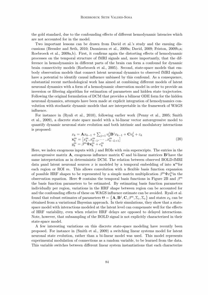
cussions (Bressler and Seth, 2010; Daunizeau et al., 2009a; David, 2009; Friston, 2009b,a;Roebroeck et al., 2009a,b). First, it confirms again the distorting effects of hemodynamicprocesses on the temporal structure of fMRI signals and, more importantly, that the dif-ference in hemodynamics in different parts of the brain can form a confound for dynamicbrain connectivity models (Roebroeck et al., 2005). Second, state-space models that em-body observation models that connect latent neuronal dynamics to observed fMRI signalshave a potential to identify causal influence unbiased by this confound. As a consequence,substantial recent methodological work has aimed at combining different models of latentneuronal dynamics with a form of a hemodynamic observation model in order to provide aninversion or filtering algorithm for estimation of parameters and hidden state trajectories.Following the original formulation of DCM that provides a bilinear ODE form for the hiddenneuronal dynamics, attempts have been made at explicit integration of hemodynamics con-volution with stochastic dynamic models that are interpretable in the framework of WAGSinfluence.For instance in (Ryali et al., 2010), following earlier work (Penny et al., 2005; Smith

et al., 2009), a discrete state space model with a bi-linear vector autoregressive model toquantify dynamic neuronal state evolution and both intrinsic and modulatory interactionsis proposed:

xk = Axk−1 +∑j=1 v

jkBjxk−1 +Cv

jk + εk

xmk =[xmk , x

mk−1, ∙ ∙ ∙ , x

mk−L+1

]

ymk = βmΦxmk + e

mk

(20)

Here, we index exogenous inputs with j and ROIs with min superscripts. The entries in theautoregressive matrix A, exogenous influence matrix C and bi-linear matrices Bjhave thesame interpretation as in deterministic DCM. The relation between observed BOLD-fMRIdata yand latent neuronal sources x is modeled by a temporal embedding of into xmforeach region or ROI m. This allows convolution with a flexible basis function expansionof possible HRF shapes to be represented by a simple matrix multiplication βmΦxmk in theobservation equation. Here Φ contains the temporal basis functions in Figure 2B and βm

the basis function parameters to be estimated. By estimating basis function parametersindividually per region, variations in the HRF shape between region can be accounted forand the confounding effects of these on WAGS influence estimate can be avoided. Ryali et al.found that robust estimates of parameters Θ =

{A,Bj ,C, βm,Σε,Σe

}and states xk can be

obtained from a variational Bayesian approach. In their simulations, they show that a state-space model with interactions modeled at the latent level can compensate well for the effectsof HRF variability, even when relative HRF delays are opposed to delayed interactions.Note, however, that subsampling of the BOLD signal is not explicitly characterized in theirstate-space model.A few interesting variations on this discrete state-space modeling have recently been

proposed. For instance in (Smith et al., 2009) a switching linear systems model for latentneuronal state evolution, rather than a bi-linear model was used. This model representsexperimental modulation of connections as a random variable, to be learned from the data.This variable switches between different linear system instantiations that each characterize

84


connectivity in a single experimental condition. Such a scheme has the important advantagethat an n-fold cross validation approach can be used to obtain a measure of absolute model-evidence (rather than relative between a selected set of models). Specifically, one couldlearn parameters for each context-specific linear system with knowledge of the timing ofchanging experimental conditions in a training data set. Then the classification accuracyof experimental condition periods in a test data set based on connectivity will provide aabsolute model-fit measure, controlled for model complexity, which can be used to validateoverall usefulness of the fitted model. In particular, this can point to important brainregions missing from the model incase of poor classification accuracy.Another related line of developments instead has involved generalizing the ODE models

in DCM for fMRI to stochastic dynamic models formulated in continuous time (Daunizeauet al., 2009b; Friston et al., 2008). An early exponent of this approach used local lineariza-tion in a (generalized) Kalman filter to estimate states and parameters in a non-linear SDEmodels of hemodynamics (Riera et al., 2004). Interestingly, the inclusion of stochastics inthe state equations makes inference on coupling parameters of such models usefully inter-pretable in the framework of WAGS influence. This hints at the ongoing convergence, inmodeling of brain connectivity, of time series approaches to causality in a discrete time tra-dition and dynamic systems and control theory approaches in a continuous time tradition.

5. Discussion and Outlook

The modeling of an enormously complex biological system such as the brain has manychallenges. The abstractions and choices to be made in useful models of brain connectivityare therefore unlikely to be accommodated by one single ‘master’ model that does betterthan all other models on all counts. Nonetheless, the ongoing development efforts towardsimproved approaches are continually extending and generalizing the contexts in which dy-namic time series models can be applied. It is clear that state space modeling and inferenceon WAGS influence are fundamental concepts within this endeavor. We end here with someconsiderations of dynamic brain connectivity models that summarize some important pointsand anticipate future developments.We have emphasized that WAGS influence models of brain connectivity have largely been

aimed at data driven exploratory analysis, whereas biophysically motivated state space mod-els are mostly used for hypothesis-led confirmatory analysis. This is especially relevant inthe interaction between model selection and model identification. Exploratory techniquesuse information in the data to investigate the relative applicability of many models. Assuch, they have the potential to detect ‘missing’ regions in anatomical models. Confirma-tory approaches test hypotheses about connectivity within a set of models assumed to beapplicable.As mentioned above, the WAGS influence approach to statistical analysis of causal influ-

ence that we focused on here is complemented by the interventional approach rooted in thetheory of graphical models and causal calculus. Graphical causal models have been recentlyapplied to brain connectivity analysis of fMRI data (Ramsey et al., 2009). Recent workcombining the two approaches (White and Lu, 2010) possibly leads the way to a combinedcausal treatment of brain imaging data incorporating dynamic models and interventions.Such a combination could enable incorporation of direct manipulation of brain activity by

85


(for example) transcranial magnetic stimulation (Pascual-Leone et al., 2000; Paus, 1999;Walsh and Cowey, 2000) into the current state space modeling framework.Causal models of brain connectivity are increasingly inspired by biophysical theories.

For fMRI this is primarily applicable in modeling the complex chain of events separatingneuronal population activity from the BOLD signal. Inversion of such a model (in statespace form) by a suitable filtering algorithm amounts to a model-based deconvolution ofthe fMRI signal resulting in an estimate of latent neuronal population activity. If thebiophysical model is appropriately formulated to be identifiable (possibly including priorson relevant parameters), it can take variation in the hemodynamics between brain regionsinto account that can otherwise confound time series causality analyses of fMRI signals.Although models of hemodynamics for causal fMRI analysis have reached a reasonablelevel of complexity, the models of neuronal dynamics used to date have remained simple,comprising one or two state variables for an entire cortical region or subcortical structure.Realistic dynamic models of neuronal activity have a long history and have reached a highlevel of sophistication (Deco et al., 2008; Markram, 2006). It remains an open issue to whatdegree complex realistic equation systems can be embedded in analysis of fMRI – or in fact:any brain imaging modality – and result in identifiable models of neuronal connectivity andcomputation.Two recent developments create opportunities to increase complexity and realism of neu-

ronal dynamics models and move the level of modeling from the macroscopic (whole brain ar-eas) towards the mesoscopic level comprising sub-populations of areas and cortical columns.First, the fusion of multiple imaging modalities, possibly simultaneously recorded, has re-ceived a great deal of attention. Particularly, several attempts to model-driven fusion ofsimultaneousy recorded fMRI and EEG data, by inverting a separate observation modelfor each modality while using the same underlying neuronal model, have been reported(Deneux and Faugeras, 2010; Riera et al., 2007; Valdes-Sosa et al., 2009). This approachholds great potential to fruitfully combine the superior spatial resolution of fMRI with thesuperior temporal resolution of EEG. In (Valdes-Sosa et al., 2009) anatomical connectivityinformation obtained from diffusion tensor imaging and fiber tractography is also incorpo-rated. Second, advances in MRI technology, particularly increases of main field strength to7T (and beyond) and advances in parallel imaging (de Zwart et al., 2006; Heidemann et al.,2006; Pruessmann, 2004; Wiesinger et al., 2006), greatly increase the level spatial detailthat are accessible with fMRI. For instance, fMRI at 7T with sufficient spatial resolution toresolve orientation columns in human visual cortex has been reported (Yacoub et al., 2008).The development of state space models for causal analysis of fMRI data has moved from

discrete to continuous and from deterministic to stochastic models. Continuous modelswith stochastic dynamics have desirable properties, chief among them a robust inferenceon causal influence interpretable in the WAGS framework, as discussed above. However,dealing with continuous stochastic models leads to technical issues such as the properties andinterpretation of Wiener processes and Ito calculus (Friston, 2008). A number of inversion orfiltering methods for continuous stochastic models have been recently proposed, particularlyfor the goal of causal analysis of brain imaging data, including the local linearization andinnovations approach (Hernandez et al., 1996; Riera et al., 2004), dynamic expectationmaximization (Friston et al., 2008) and generalized filtering (Friston et al., 2010). The

86


ongoing development of these filtering methods, their validation and their scalability towardslarge numbers of state variables will be a topic of continuing research.

Acknowledgments

The authors thank Kamil Uludag for comments and discussion.

References

Odd O. Aalen. Dynamic modeling and causality. Scandinavian Actuarial journal, pages177–190, 1987.

O.O. Aalen and A. Frigessi. What can statistics contribute to a causal understanding?Board of the Foundation of the Scandinavian journal of Statistics, 34:155–168, 2007.

G. K. Aguirre, E. Zarahn, and M. D’Esposito. The variability of human, bold hemodynamicresponses. Neuroimage, 8(4):360–9, 1998.

H Akaike. On the use of a linear model for the identification of feedback systems. Annalsof the Institute of statistical mathematics, 20(1):425–439, 1968.

A Amendola, M Niglio, and C Vitale. Temporal aggregation and closure of varma models:Some new results. In F. Palumbo et al., editor, Data Analysis and Classification: Studiesin Classification, Data Analysis, and Knowledge Organization, pages 435–443. 2010.

D. Attwell, A. M. Buchan, S. Charpak, M. Lauritzen, B. A. Macvicar, and E. A. Newman.Glial and neuronal control of brain blood flow. Nature, 468(7321):232–43, 2010.

D. Attwell and C. Iadecola. The neural basis of functional brain imaging signals. TrendsNeurosci, 25(12):621–5, 2002.

A. B. Barrett, L. Barnett, and A. K. Seth. Multivariate granger causality and generalizedvariance. Phys Rev E Stat Nonlin Soft Matter Phys, 81(4 Pt 1):041907, 2010.

M.J. Beal. Variational Algorithms for Approximate Bayesian Inference. PhD thesis, Uni-versity College London, 2003.

A R Bergstrom. Nonrecursive models as discrete approximations to systems of stochasticdifferential equations. Econometrica, 34:173–182, 1966.

A R Bergstrom. Continuous time stochastic models and issues of aggregation. In Z. Grilichesand M.D. Intriligator, editors, Handbook of econometrics, volume II. Elsevier, 1984.

M.A. Bernstein, K.F. King, and X.J. Zhou. Handbook of MRI Pulse Sequences. ElsevierAcademic Press, urlington, 2004.

S. L. Bressler and A. K. Seth. Wiener-granger causality: A well established methodology.Neuroimage, 2010.

87


S. L. Bressler, W. Tang, C. M. Sylvester, G. L. Shulman, and M. Corbetta. Top-downcontrol of human visual cortex by frontal and parietal cortex in anticipatory visual spatialattention. J Neurosci, 28(40):10056–61, 2008.

R. B. Buxton. The elusive initial dip. Neuroimage, 13(6 Pt 1):953–8, 2001.

R. B. Buxton, K. Uludag, D. J. Dubowitz, and T. T. Liu. Modeling the hemodynamicresponse to brain activation. Neuroimage, 23 Suppl 1:S220–33, 2004.

R. B. Buxton, E. C. Wong, and L. R. Frank. Dynamics of blood flow and oxygenationchanges during brain activation: the balloon model. Magn Reson Med, 39(6):855–64,1998.

Marcus J Chambers and Michael A Thornton. Discrete time representation of continuoustime arma processes, 2009.

Daniel Commenges and Anne Gegout-Petit. A general dynamical statistical model with pos-sible causal interpretation. journal of the Royal Statistical Society: Series B (StatisticalMethodology), 71(3):1–43, 2009.

J. Daunizeau, O. David, and K. E. Stephan. Dynamic causal modelling: A critical reviewof the biophysical and statistical foundations. Neuroimage, 2009a.

J. Daunizeau, K. J. Friston, and S. J. Kiebel. Variational bayesian identification and pre-diction of stochastic nonlinear dynamic causal models. Physica D, 238(21):2089–2118,2009b.

O. David. fmri connectivity, meaning and empiricism comments on: Roebroeck et al. theidentification of interacting networks in the brain using fmri: Model selection, causalityand deconvolution. Neuroimage, 2009.

O. David, I. Guillemain, S. Saillet, S. Reyt, C. Deransart, C. Segebarth, and A. Depaulis.Identifying neural drivers with functional mri: an electrophysiological validation. PLoSBiol, 6(12):2683–97, 2008.

J. A. de Zwart, P. van Gelderen, X. Golay, V. N. Ikonomidou, and J. H. Duyn. Acceleratedparallel imaging for functional imaging of the human brain. NMR Biomed, 19(3):342–51,2006.

G. Deco, V. K. Jirsa, P. A. Robinson, M. Breakspear, and K. Friston. The dynamic brain:from spiking neurons to neural masses and cortical fields. PLoS Comput Biol, 4(8):e1000092, 2008.

T. Deneux and O. Faugeras. Eeg-fmri fusion of paradigm-free activity using kalman filtering.Neural Comput, 22(4):906–48, 2010.

G. Deshpande, X. Hu, R. Stilla, and K. Sathian. Effective connectivity during hapticperception: a study using granger causality analysis of functional magnetic resonanceimaging data. Neuroimage, 40(4):1807–14, 2008.

88


G. Deshpande, S. LaConte, G. A. James, S. Peltier, and X. Hu. Multivariate grangercausality analysis of fmri data. Hum Brain Mapp, 30(4):1361–73, 2009.

G. Deshpande, K. Sathian, and X. Hu. Effect of hemodynamic variability on grangercausality analysis of fmri. Neuroimage, 52(3):884–96, 2010.

J Florens. Some technical issues in defning causality. journal of Econometrics, 112:127–128,2003.

J.P. Florens and D. Fougere. Noncausality in continuous time. Econometrica, 64(5):1195–1212, 1996.

K. Friston. Functional and effective connectivity in neuroimaging: A synthesis. Hum BrainMapp, 2:56–78, 1994.

K. Friston. Beyond phrenology: what can neuroimaging tell us about distributed circuitry?Annu Rev Neurosci, 25:221–50, 2002.

K. Friston. Dynamic causal modeling and granger causality comments on: The identifi-cation of interacting networks in the brain using fmri: Model selection, causality anddeconvolution. Neuroimage, 2009a.

K. Friston, J. Mattout, N. Trujillo-Barreto, J. Ashburner, and W. Penny. Variational freeenergy and the laplace approximation. Neuroimage, 34(1):220–34, 2007.

K. J. Friston, L. Harrison, and W. Penny. Dynamic causal modelling. Neuroimage, 19(4):1273–302, 2003.

K. J. Friston, A. Mechelli, R. Turner, and C. J. Price. Nonlinear responses in fmri: theballoon model, volterra kernels, and other hemodynamics. Neuroimage, 12(4):466–77,2000.

K. J. Friston, N. Trujillo-Barreto, and J. Daunizeau. Dem: a variational treatment ofdynamic systems. Neuroimage, 41(3):849–85, 2008.

Karl Friston. Hierarchical models in the brain. PLoS Computational Biology, 4, 2008.

Karl Friston. Causal modelling and brain connectivity in functional magnetic resonanceimaging. PLoS biology, 7:e33, 2009b.

Karl Friston, Klaas Stephan, Baojuan Li, and Jean Daunizeau. Generalised filtering. Math-ematical Problems in Engineering, 2010:1–35, 2010.

J. F. Geweke. Measurement of linear dependence and feedback between multiple time series.journal of the American Statistical Association, 77(378):304–324, 1982.

G. H. Glover. Deconvolution of impulse response in event-related bold fmri. Neuroimage,9(4):416–29, 1999.

C. Glymour. Learning, prediction and causal bayes nets. Trends Cogn Sci, 7(1):43–48, 2003.

89


R. Goebel, A. Roebroeck, D. S. Kim, and E. Formisano. Investigating directed corticalinteractions in time-resolved fmri data using vector autoregressive modeling and grangercausality mapping. Magn Reson Imaging, 21(10):1251–61, 2003.

C. W. J. Granger. Investigating causal relations by econometric models and cross-spectralmethods. Econometrica, 37(3):424–438, 1969.

E.M. Haacke, R.W. Brown, M.R. Thompson, and R. Venkatesan. Magnetic ResonanceImaging: Physical Principles and Sequence Design. John Wiley and Sons, Inc, NewYork, 1999.

M. Havlicek, J. Jan, M. Brazdil, and V. D. Calhoun. Dynamic granger causality based onkalman filter for evaluation of functional network connectivity in fmri data. Neuroimage,53(1):65–77, 2010.

R. M. Heidemann, N. Seiberlich, M. A. Griswold, K. Wohlfarth, G. Krueger, and P. M.Jakob. Perspectives and limitations of parallel mr imaging at high field strengths. Neu-roimaging Clin N Am, 16(2):311–20, 2006.

R. N. Henson, C. J. Price, M. D. Rugg, R. Turner, and K. J. Friston. Detecting latencydifferences in event-related bold responses: application to words versus nonwords andinitial versus repeated face presentations. Neuroimage, 15(1):83–97, 2002.

JL Hernandez, PA Valds, and P Vila. Eeg spike and wave modelled by a stochastic limitcycle. NeuroReport, 1996.

B. Horwitz, K. J. Friston, and J. G. Taylor. Neural modeling and functional brain imaging:an overview. Neural Netw, 13(8-9):829–46, 2000.

H. Johansen-Berg and T.E.J Behrens, editors. Diffusion MRI: From quantitative measure-ment to in-vivo neuroanatomy. Academic Press, London, 2009.

D.K. Jones, editor. Diffusion MRI: Theory, Methods, and Applications. Oxford UniversityPress, Oxford, 2010.

S. J. Kiebel, M. I. Garrido, R. Moran, C. C. Chen, and K. J. Friston. Dynamic causalmodeling for eeg and meg. Hum Brain Mapp, 30(6):1866–76, 2009.

C. H. Liao, K. J. Worsley, J. B. Poline, J. A. Aston, G. H. Duncan, and A. C. Evans.Estimating the delay of the fmri response. Neuroimage, 16(3 Pt 1):593–606, 2002.

L. Ljung. System Identification: Theory for the User. Prentice-Hall, New Jersey, 2ndedition, 1999.

N. K. Logothetis. What we can do and what we cannot do with fmri. Nature, 453(7197):869–78, 2008.

N. K. Logothetis, J. Pauls, M. Augath, T. Trinath, and A. Oeltermann. Neurophysiologicalinvestigation of the basis of the fmri signal. Nature, 412(6843):150–7, 2001.

H. Markram. The blue brain project. Nat Rev Neurosci, 7(2):153–60, 2006.

90


A. C. Marreiros, S. J. Kiebel, and K. J. Friston. Dynamic causal modelling for fmri: atwo-state model. Neuroimage, 39(1):269–78, 2008.

J. Roderick McCrorie. The likelihood of the parameters of a continuous time vector autore-gressive model. Statistical Inference for Stochastic Processes, 5:273–286, 2002.

J. Roderick Mccrorie. The problem of aliasing in identifying finite parameter continuoustime stochastic models. Acta Applicandae Mathematicae, 79:9–16, 2003.

A. R. McIntosh. Contexts and catalysts: a resolution of the localization and integration offunction in the brain. Neuroinformatics, 2(2):175–82, 2004.

T Ozaki. A bridge between nonlinear time series models and nonlinear stochastic dynamicalsystems: A local linearization approach. Statistica Sinica, 2:113–135, 1992.

A. Pascual-Leone, V. Walsh, and J. Rothwell. Transcranial magnetic stimulation in cog-nitive neuroscience–virtual lesion, chronometry, and functional connectivity. Curr OpinNeurobiol, 10(2):232–7, 2000.

T. Paus. Imaging the brain before, during, and after transcranial magnetic stimulation.Neuropsychologia, 37(2):219–24, 1999.

J. Pearl. Causality: Models, Reasoning and Inference. Cambridge University Press, NewYork, 2nd edition, 2009.

W. Penny, Z. Ghahramani, and K. Friston. Bilinear dynamical systems. Philos Trans RSoc Lond B Biol Sci, 360(1457):983–93, 2005.

W. D. Penny, K. E. Stephan, A. Mechelli, and K. J. Friston. Comparing dynamic causalmodels. Neuroimage, 22(3):1157–72, 2004.

Peter C.B. Phillips. The problem of identification in finite parameter continous time models.journal of Econometrics, 1:351–362, 1973.

Peter C.B. Phillips. The estimation of some continuous time models. Econometrica, 42:803–823, 1974.

K. P. Pruessmann. Parallel imaging at high field strength: synergies and joint potential.Top Magn Reson Imaging, 15(4):237–44, 2004.

J. D. Ramsey, S. J. Hanson, C. Hanson, Y. O. Halchenko, R. A. Poldrack, and C. Glymour.Six problems for causal inference from fmri. Neuroimage, 49(2):1545–58, 2009.

A. Rauch, G. Rainer, and N. K. Logothetis. The effect of a serotonin-induced dissociationbetween spiking and perisynaptic activity on bold functional mri. Proc Natl Acad Sci US A, 105(18):6759–64, 2008.

G.C. Reinsel. Elements of Multivariate Time Series Analysis. Springer-Verlag, New York,2nd edition, 1997.

91


J. J. Riera, J. C. Jimenez, X. Wan, R. Kawashima, and T. Ozaki. Nonlinear local elec-trovascular coupling. ii: From data to neuronal masses. Hum Brain Mapp, 28(4):335–54,2007.

J. J. Riera, J. Watanabe, I. Kazuki, M. Naoki, E. Aubert, T. Ozaki, and R. Kawashima.A state-space model of the hemodynamic approach: nonlinear filtering of bold signals.Neuroimage, 21(2):547–67, 2004.

A. Roebroeck, E. Formisano, and R. Goebel. Mapping directed influence over the brainusing granger causality and fmri. Neuroimage, 25(1):230–42, 2005.

A. Roebroeck, E. Formisano, and R. Goebel. The identification of interacting networks inthe brain using fmri: Model selection, causality and deconvolution. Neuroimage, 2009a.

A. Roebroeck, E. Formisano, and R. Goebel. Reply to friston and david after commentson: The identification of interacting networks in the brain using fmri: Model selection,causality and deconvolution. Neuroimage, 2009b.

S. Ryali, K. Supekar, T. Chen, and V. Menon. Multivariate dynamical systems models forestimating causal interactions in fmri. Neuroimage, 2010.

Z. S. Saad, K. M. Ropella, R. W. Cox, and E. A. DeYoe. Analysis and use of fmri responsedelays. Hum Brain Mapp, 13(2):74–93, 2001.

R. Salmelin and J. Kujala. Neural representation of language: activation versus long-rangeconnectivity. Trends Cogn Sci, 10(11):519–25, 2006.

J. R. Sato, A. Fujita, E. F. Cardoso, C. E. Thomaz, M. J. Brammer, and Jr. E. Amaro.Analyzing the connectivity between regions of interest: an approach based on clustergranger causality for fmri data analysis. Neuroimage, 52(4):1444–55, 2010.

J. R. Sato, D. Y. Takahashi, S. M. Arcuri, K. Sameshima, P. A. Morettin, and L. A.Baccala. Frequency domain connectivity identification: an application of partial directedcoherence in fmri. Hum Brain Mapp, 30(2):452–61, 2009.

M. B. Schippers, A. Roebroeck, R. Renken, L. Nanetti, and C. Keysers. Mapping theinformation flow from one brain to another during gestural communication. Proc NatlAcad Sci U S A, 107(20):9388–93, 2010.

T Schweder. Composable markov processes. journal of Applied Probability, 7(2):400–410,1970.

J. F. Smith, A. Pillai, K. Chen, and B. Horwitz. Identification and validation of effectiveconnectivity networks in functional magnetic resonance imaging using switching lineardynamic systems. Neuroimage, 52(3):1027–40, 2009.

S. M. Smith, K. L. Miller, G. Salimi-Khorshidi, M. Webster, C. F. Beckmann, T. E. Nichols,J. D. Ramsey, and M. W. Woolrich. Network modelling methods for fmri. Neuroimage,2010.

92


V Solo. On causality i: Sampling and noise. Proceedings of the 46th IEEE Conference onDecision and Control, pages 3634–3639, 2006.

D. Sridharan, D. J. Levitin, and V. Menon. A critical role for the right fronto-insular cortexin switching between central-executive and default-mode networks. Proc Natl Acad SciU S A, 105(34):12569–74, 2008.

K. E. Stephan, L. Kasper, L. M. Harrison, J. Daunizeau, H. E. den Ouden, M. Breakspear,and K. J. Friston. Nonlinear dynamic causal models for fmri. Neuroimage, 42(2):649–62,2008.

I. H. Stevenson and K. P. Kording. On the similarity of functional connectivity betweenneurons estimated across timescales. PLoS One, 5(2):e9206, 2010.

K. Thomsen, N. Offenhauser, and M. Lauritzen. Principal neuron spiking: neither necessarynor sufficient for cerebral blood flow in rat cerebellum. J Physiol, 560(Pt 1):181–9, 2004.

L. Q. Uddin, A. M. Kelly, B. B. Biswal, F. Xavier Castellanos, and M. P. Milham. Func-tional connectivity of default mode network components: correlation, anticorrelation, andcausality. Hum Brain Mapp, 30(2):625–37, 2009.

K. Ugurbil, L. Toth, and D. S. Kim. How accurate is magnetic resonance imaging of brainfunction? Trends Neurosci, 26(2):108–14, 2003.

K. Uludag. To dip or not to dip: reconciling optical imaging and fmri data. Proc Natl AcadSci U S A, 107(6):E23; author reply E24, 2010.

K. Uludag, D. J. Dubowitz, and R. B. Buxton. Basic principles of functional mri. InR. Edelman, J. Hesselink, and M. Zlatkin, editors, Clinical MRI. Elsevier, San Diego,2005.

K. Uludag, B. Muller-Bierl, and K. Ugurbil. An integrative model for neuronal activity-induced signal changes for gradient and spin echo functional imaging. Neuroimage, 48(1):150–65, 2009.

P Valdes-Sosa, J C Jimenez, J Riera, R Biscay, and T Ozaki. Nonlinear eeg analysis basedon a neural mass model. Biological cybernetics, 81:415–24, 1999.

P. Valdes-Sosa, A. Roebroeck, J. Daunizeau, and K. Friston. Effective connectivity: Influ-ence, causality and biophysical modeling. Neuroimage, in press.

P. A. Valdes-Sosa. Spatio-temporal autoregressive models defined over brain manifolds.Neuroinformatics, 2(2):239–50, 2004.

P. A. Valdes-Sosa, R. Kotter, and K. J. Friston. Introduction: multimodal neuroimaging ofbrain connectivity. Philos Trans R Soc Lond B Biol Sci, 360(1457):865–7, 2005a.

P. A. Valdes-Sosa, J. M. Sanchez-Bornot, A. Lage-Castellanos, M. Vega-Hernandez,J. Bosch-Bayard, L. Melie-Garcia, and E. Canales-Rodriguez. Estimating brain func-tional connectivity with sparse multivariate autoregression. Philos Trans R Soc Lond BBiol Sci, 360(1457):969–81, 2005b.

93


P. A. Valdes-Sosa, J. M. Sanchez-Bornot, R. C. Sotero, Y. Iturria-Medina, Y. Aleman-Gomez, J. Bosch-Bayard, F. Carbonell, and T. Ozaki. Model driven eeg/fmri fusion ofbrain oscillations. Hum Brain Mapp, 30(9):2701–21, 2009.

V. Walsh and A. Cowey. Transcranial magnetic stimulation and cognitive neuroscience. NatRev Neurosci, 1(1):73–9, 2000.

W. W. S. Wei. Time Series Analysis: Univariate and Multivariate Methods. Addison-Wesley, Redwood City, 1990.

Halbert White and Xun Lu. Granger causality and dynamic structural systems. Journal ofFinancial Econometrics, 8(2):193–243, 2010.

N. Wiener. The theory of prediction. In E.F. Berkenbach, editor, Modern Mathematics forEngineers. McGraw-Hill, New York, 1956.

F. Wiesinger, P. F. Van de Moortele, G. Adriany, N. De Zanche, K. Ugurbil, and K. P.Pruessmann. Potential and feasibility of parallel mri at high field. NMR Biomed, 19(3):368–78, 2006.

E. Yacoub, N. Harel, and K. Ugurbil. High-field fmri unveils orientation columns in humans.Proc Natl Acad Sci U S A, 105(30):10607–12, 2008.

94

Date post:	31-Dec-2016
Category:	Documents
Upload:	vuongkhanh
View:	226 times
Download:	0 times

Causal Time Series Analysis of functional Magnetic Resonance ...

Documents