Page 1
Cavity QED with a Large Mode
Volume High Finesse Cavity
An Experimental Challenge
Dissertation
zur Erlangung des Doktorgrades
des Fachbereichs Physik
der Universität Hamburg
vorgelegt von
Leif Malik Lindholdt
aus uuk (Dänemark)
Hamburg 2009
Page 2
1
Gutachter der Dissertation : Prof. Dr. A. Hemmerich
: Prof. Dr. W. Neuhauser
Gutachter der Disputation : Prof. Dr. A. Hemmerich
: Prof. Dr. K. Sengstock
Vorsitzender des Prüfungsausschusses : Prof. Dr. W. Hansen
Vorsitzender des Promotionsausschusses : Prof. Dr. R. Klanner
Page 3
2
Table of contents
1 Introduction....................................................................................5
2 Theoretical basis ............................................................................9
2.1 Atomic properties for Rb87...................................................................................... 10
2.2 Magnetic optical trap................................................................................................ 12
2.3 Magnetic traps .......................................................................................................... 13
2.4 Evaporative cooling.................................................................................................. 17
2.5 A dilute Bose gas in a harmonic potential................................................................ 21
2.6 Absorption imaging.................................................................................................. 25
3 Cavity theory................................................................................27
3.1 Gaussian beams ........................................................................................................ 27
3.2 Cavity stability ......................................................................................................... 28
3.3 Cavity incoupling ..................................................................................................... 30
3.4 Cavity enhancement ................................................................................................. 32
3.5 Scattering enhancement............................................................................................ 33
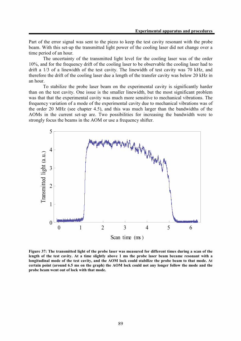
4 Cavity/atom interaction ..............................................................35
4.1 Optical dipole trap.................................................................................................... 35
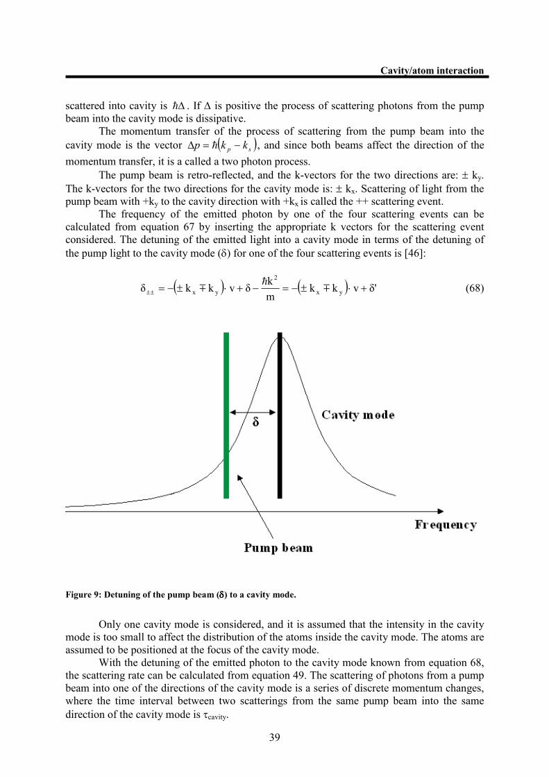
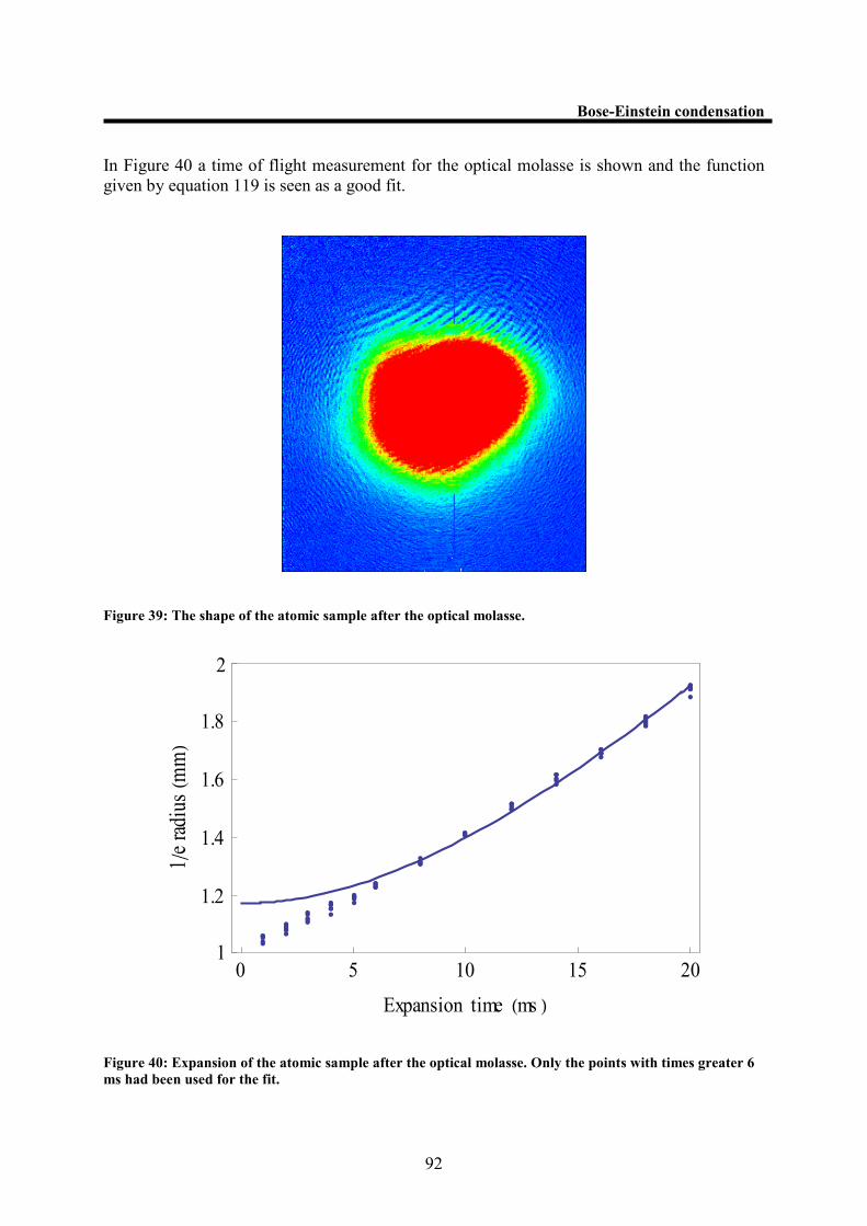
4.2 Cavity Doppler cooling ............................................................................................ 38
4.3 Self-organization of atoms in a cavity...................................................................... 44
4.4 Cavity sideband cooling ........................................................................................... 51
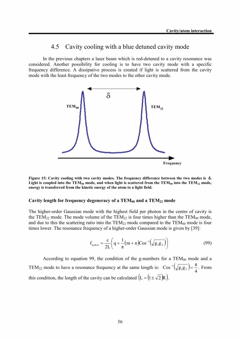
4.5 Cavity cooling with a blue detuned cavity mode ..................................................... 56
4.6 Normal mode splitting of a ring cavity mode .......................................................... 57
Page 4
3
Table of contents
5 Experiment apparatus and procedures.....................................65
5.1 Laser stabilization .................................................................................................... 65
5.2 Atom source ............................................................................................................. 68
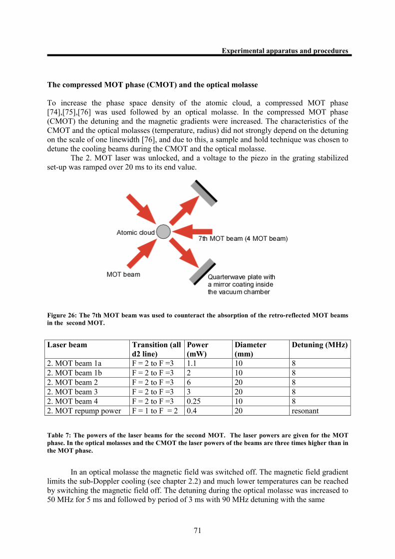
5.3 The second MOT...................................................................................................... 70
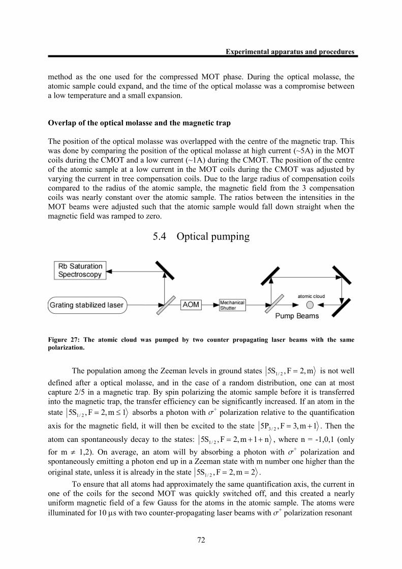
5.4 Optical pumping....................................................................................................... 72
5.5 Magnetic trapping .................................................................................................... 73
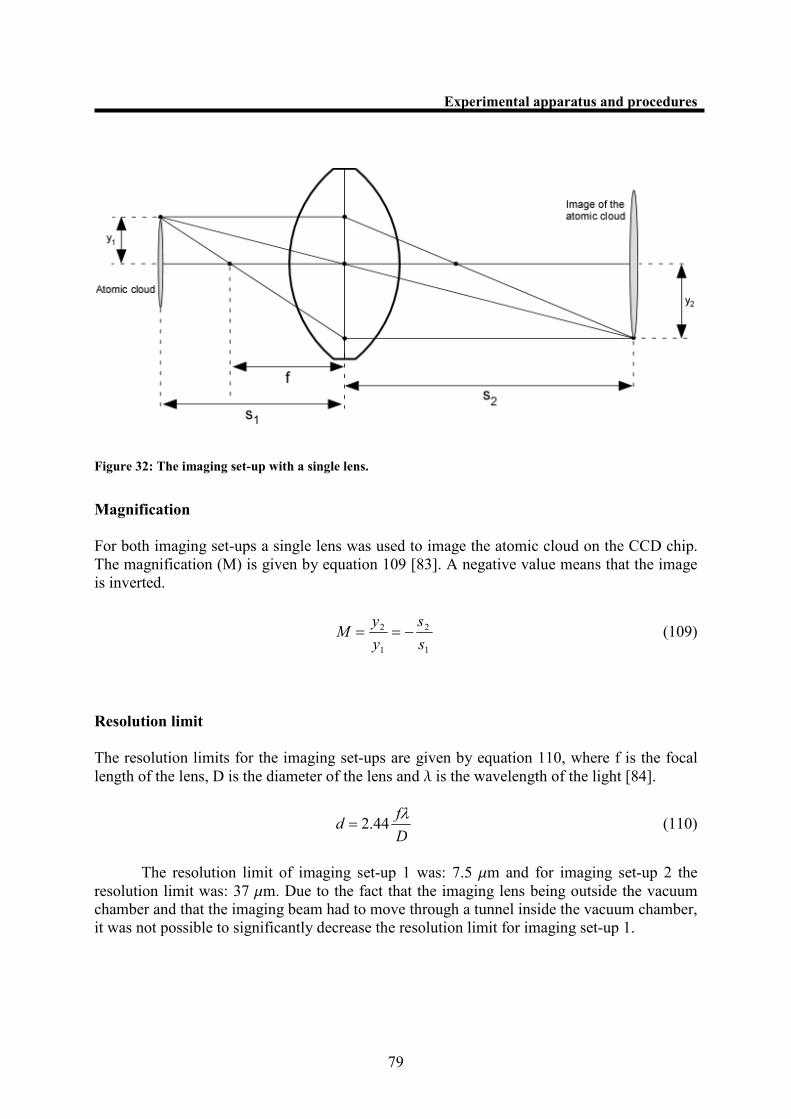
5.6 Imaging system ........................................................................................................ 78
5.7 The Vacuum Chamber ............................................................................................. 81
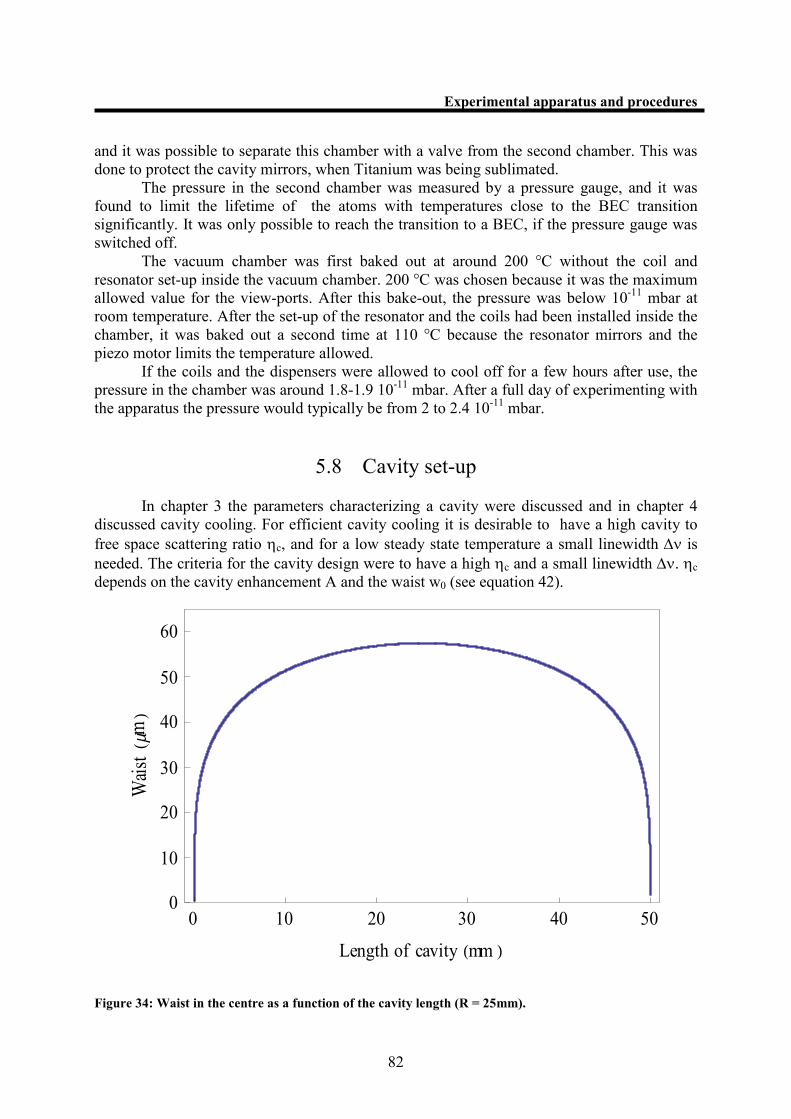
5.8 Cavity set-up ............................................................................................................ 82
5.9 Radio frequency source............................................................................................ 84
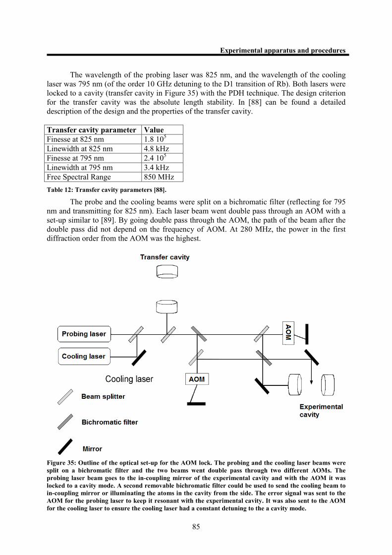
5.10 AOM Lock ............................................................................................................... 84
6 Bose-Einstein Condensation .......................................................90
6.1 Preparation of the atomic sample for the magnetic trap........................................... 90
6.2 The Magnetic traps................................................................................................... 93
6.3 Evaporative cooling.................................................................................................. 95
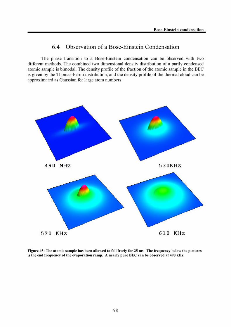
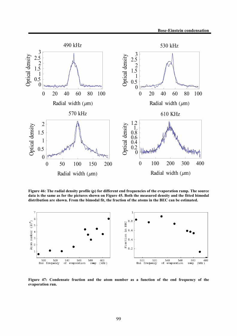
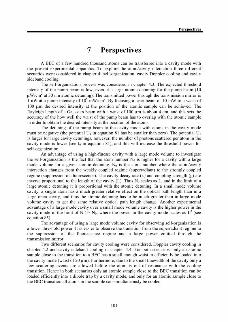
6.4 Observation of a Bose-Einstein Condensation......................................................... 98
7 Perspectives ................................................................................101
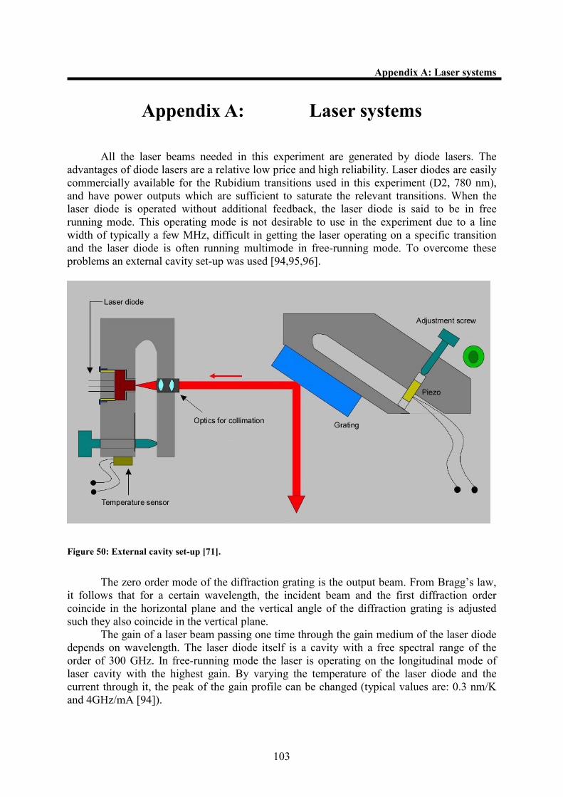
Appendix A: Laser systems ......................................................103
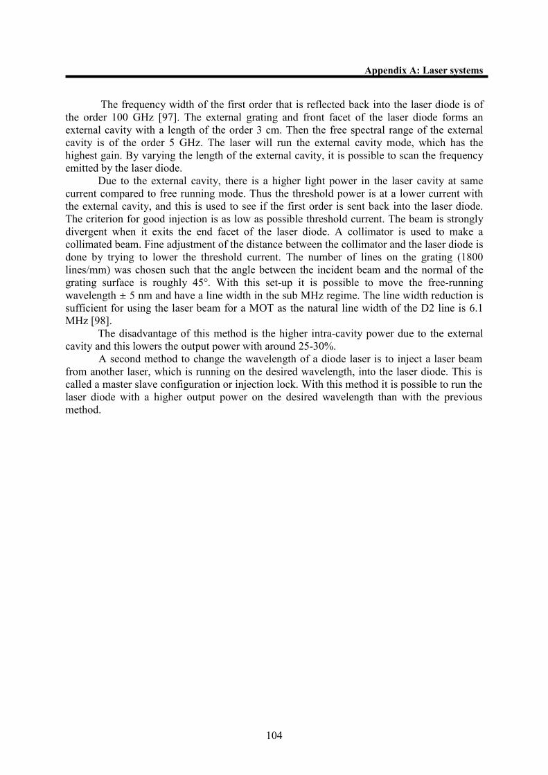
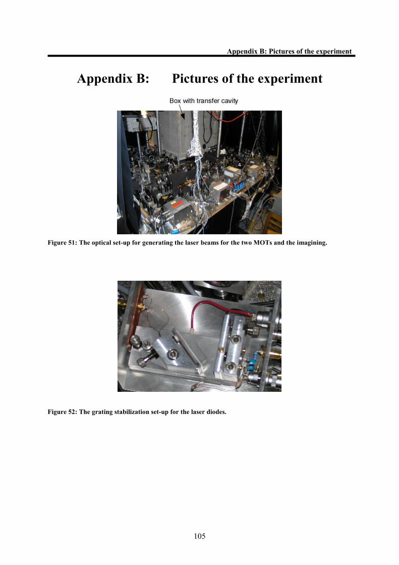
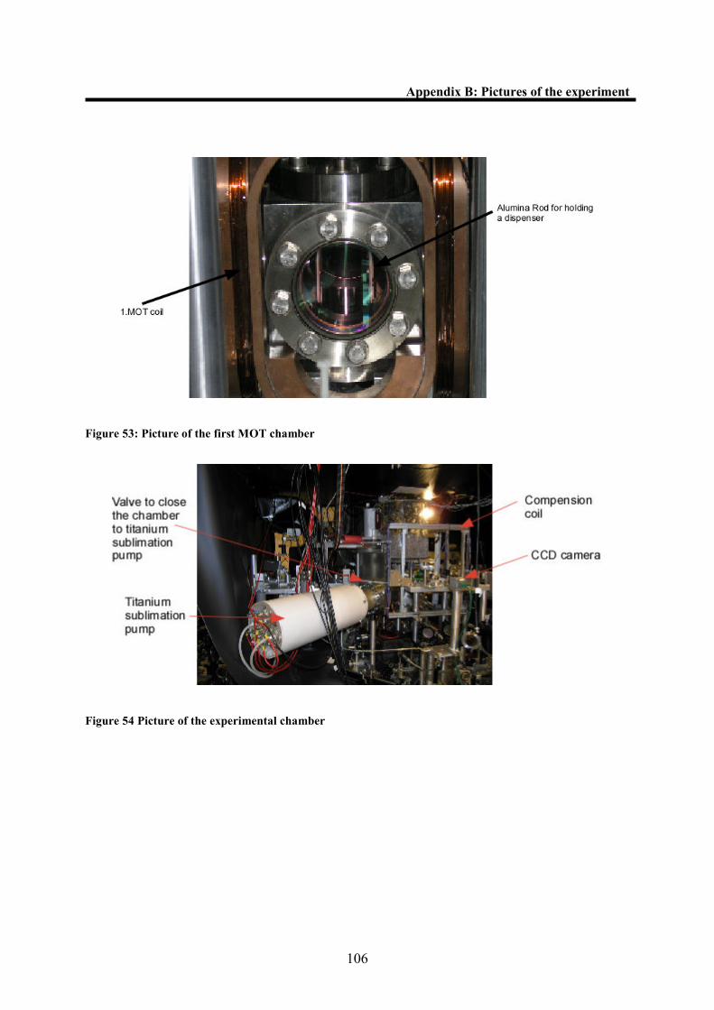
Appendix B: Pictures of the experiment ..................................105
Acknowledgement............................................................................108
Bibliography.....................................................................................109
Page 5
4
Summary
Summary
This thesis deals with the interaction between a cold quantum gas and the photons of a
high finesse cavity mode. The regime of strong coupling was first explored by measuring the
normal mode splitting of a ring cavity mode. In the last decade many interesting scenarios,
like cavity Doppler cooling, cavity sideband cooling and self organization of atoms were
predicted theoretically. Demonstrating these effects with a large number of atoms at extreme
low temperatures require a cavity with a very high finesse and a large mode volume.
Thus an experimental apparatus was built that allows overlapping a BEC of a few 105
rubidium atoms with a cavity mode with a large mode volume. To explore the regime of
strong coupling a moderate detuning from the atomic resonance and a cavity with a finesse of
more than 400000 was chosen. The cavity has an adjustable length and can be adjusted to be
nearly spherical. With a cavity to free space scattering ratio up to 20 cavity Doppler cooling,
cavity sideband cooling and self organization of atoms should be accessible. The relevant
quantities for these scenarios are calculated and the feasibility of a experimental realisation is
discussed.
Zusammenfassung
Diese Arbeit behandelt die Wechselwirkung zwischen einem kalten Quantengas und
den Photonen einer Mode eines Hochfinesse-Resonators. Das Regime der starken Kopplung
wurde zunaächst anhand der Modenaufspaltung in einem Ringresonator untersucht. Im
vergangenen Jahrzehnt wurden viele interessante Szenarien, wie Resonator-Dopplerkühlung,
Resonator-Seitenbandkühlung und Selbstorganisation von Atomen theoretisch vorhergesagt.
Um diese Effekte mit einer grossen Anzahl von Atomen bei extrem niedrigen
Temperaturen experimentell zu demonstrieren, braucht man einen Resonator mit einer sehr
grossen Finesse und einem grossen Modenvolumen.
Daher wurde eine Apparatur aufgebaut, die es erlaubt ein BEC, das aus einigen 10^5
Atomen besteht, mit einer Resonatormode mit grossem Modenvolumen zu überlagern. Um in
das Regime der starken Kopplung zu gelangen, wurde eine moderate Verstimmung von der
Atomresonanz und ein Resonator mit einer Finesse von mehr als 400000 verwendet. Der
Resonator ist längenverstellbar und kann so eingestellt werden, dass er fast sphärisch ist. Mit
einem Verhältnis aus Streuung in den freien Raum zu Streuung in die Resonatormode von 20,
sollte es möglich sein Resonator-Dopplerkühlung, Resonator-Seitenbandkühlung und
Selbstorganisation zu erreichen. Die entscheidenden physikalischen Grössen für diese
Szenarien werden berechnet und die experimentelle Realsierbarkeit wird diskutiert.
Page 6
5
Introduction
1 Introduction
Optics is the study of properties of light and its interaction with matter. Among the
many research fields in optics this thesis focuses on the study of a single radiation mode
interacting with an atomic sample. A resonator can be used to enhance the scattering
probability of an atom at certain frequencies and suppress it at other frequencies. If this
frequency selection is sufficiently good, an atom inside a resonator only interacts with a
single radiation mode.
The development of the single atom maser (micromaser) in the 1980s allowed a
detailed study of the interaction between a single highly excited atom and a single radiation
mode in the microwave regime [1,2]. The study of single atoms interacting with a single
resonant radiation mode has expanded to the optical domain, and of particular interest for the
topics discussed in this thesis can be mentioned cavity cooling of a single atom [3].
A different regime to explore is the interaction between a resonator mode and a dilute
atomic gas. The atomic samples created in a magnetic optical trap have such a high density
that many atoms overlap well with a resonator mode. An early experimental observation was
made in 1995 with an atomic sample from a magnetic optical trap overlapped with a resonator
mode [4]. Due to the relative low finesse (~100) the radiation mode had to be resonant with
an atomic transition to observe an interaction between the radiation mode and the atomic
sample.
In the end of the 1990s it became technically possible to create mirrors with only a few
ppm losses per reflection. Thus it became possible to reach the strongly coupled regime with a
resonator mode far detuned from an atomic resonance (the dispersive regime) and an atomic
sample of a few million atoms. In the strongly coupled regime the scattering of photons by
atoms into a resonator mode dominates over all other scattering processes. The dynamics
between a cold atomic sample extracted from a magnetic optical trap and a far detuned
resonator mode was first investigated with ring-cavities and interesting phenomena as
collective atom recoil lasing (CARL) [5], optical bistability [] and the normal mode splitting
of a resonator mode in the dispersive regime [65] have been observed. The measurement of
the normal mode splitting is discussed in this thesis.
In the last few years efforts have been made to study the interaction between a Bose-
Einstein condensate and a resonator mode [6,7,8]. In a Bose-Einstein condensate all atoms are
in the ground state and thus all the atoms have the same wavefunction. This is analogous to a
laser beam where all the photons have the same state, and an atomic beam extracted from a
Bose-Einstein is referred to as an atom laser. The interaction of a Bose-Einstein condensate
and a resonator mode can be used for non-demolition measurement on the Bose-Einstein
condensate [92], or to cool excitations of a Bose-Einstein condensate.
The experimental apparatus
To explore the interaction between a Bose-Einstein condensate and a resonator mode, an
experimental apparatus was built as part of this thesis, and this experimental apparatus allows
a Bose-Einstein condensate to be overlapped with a resonator mode of a high finesse cavity.
What sets the cavity presented in this thesis apart from other experiments with high-
finesse cavities and a Bose-Einstein condensate is a small linewidth of a few kHz. The small
linewidth makes the resonator ideally suited for cavity cooling near the recoil limit.
Page 7
6
Introduction
Cavity cooling
A cooling scheme using a resonator mode is known as cavity cooling. The principle in cavity
cooling is the same as the one for laser cooling on an atomic resonance, the atom absorbs a
photon with less energy than the one it on average emits. For far detuned light, the number of
spontaneous emissions by the atoms can be small, and thus the probability for the atom to
change its internal state during the time period where the atom is cooled by the light can also
be made small. The fact that the internal state of the atom can remain unchanged in the
cooling process is a potential major advance of cavity cooling over laser cooling on an atomic
transition, and in principle every particle that is polarizable can be cooled with cavity cooling.
Another advantage of not having resonant photons in the cooling process is the fact that the
maximum density is not limited by an internal light pressure of resonant photons as it is the
case in a magnetic optical trap.
In laser cooling the steady state temperature depends on the linewidth of the cooling
transition and the linewidths of the atomic transitions, typically used in laser cooling, are a
few MHz and this corresponds to a temperature of 100 µK. The linewidth of a resonator mode
can be made arbitrarily small in theory and for a large open cavity with a length of a few
centimetres a linewidth of a few kHz is technically achievable. With a steady state
temperature near the recoil limit it would be possible to cool an atomic sample to a Bose-
Einstein condensate without the loss of atoms as in evaporative cooling.
The advantages of using a cavity resonance instead of an atomic resonance for laser
cooling are: in principle every polarizable particle can be cooled, practical no density
limitation and the possibility to cool an atomic sample to the recoil temperature without any
loss of atoms.
Two different scenarios for cavity cooling are considered in this thesis, Doppler
cooling and sideband cooling. Doppler cooling uses free atoms, and it is similar to Doppler
cooling on an atomic resonance. Cavity sideband cooling is for bound atoms in a harmonic
potential.
Self-organization of an atomic sample
In [51] an organization process (self-organization) is discussed in which an initial even atomic
distribution is changed to a Bragg grating structure with the periodicity of the wavelength of
an illuminating laser beam. In this type of distribution all photons emitted by the atoms will
constructively interfere with each other, and this will significantly increase the scattering rate
into the cavity mode. As a scattering event into the cavity mode typically is a cooling process,
the ordering of atoms into a distribution with periodicity of one wavelength promises to be a
method which could significantly improve cavity cooling.
In [53] experimental evidence of such a process has been observed. When the
atom/cavity interaction is in the strongly coupled regime the illuminating light and light field
in the cavity mode are predicted to destructively interfere with similar amplitudes [55]. In this
case the fluorescence of atoms is strongly suppressed. In the limit of weak coupling the self-
organization process will strongly enhance scattering into the cavity mode and therefore
significantly increase the cooling rate. In the strong coupled regime it is be possible to hold
atoms at very low intensity. Due to the low scattering rate in this configuration, the atoms can
be held at very low temperatures.
Page 8
7
Introduction
Measurement of the normal mode splitting with a far detuned probe
The results of the measurements of the normal mode splitting in the strongly coupled regime
with a far detuned probe beam are presented in this thesis [94]. The experimental apparatus
used for this measurement is the previous cavity experiment in the group [65,71]. The
experimental apparatus consisted of a ring cavity where a cold atomic sample could be loaded
into the modes of a ring cavity from a MOT. With this experimental apparatus optical
bistability was observed [9], however, it was not possible to observe cavity cooling with this
experimental set-up. The primary reason for this is believed to be that the scattering rate into
the cavity mode was comparable to the scattering rate into free space. Thus, one of the criteria
for the design of the experimental apparatus presented in this thesis was to have a high ratio
of the scattering rate into the cavity modes compared to the scattering rate into free space.
Collective side band cooling
An interesting variation of the cavity cooling scenario is the possibility to use a second cavity
mode instead of a detuned laser beam to a cavity resonance to create a dissipative process. In
[61] the possibility to use the normal mode splitting for a cooling scheme is discussed
(collective sideband cooling). The normal mode splitting has previously been measured with a
near-resonant probe beam [62,63], however, one of the major advantages of cavity cooling is
the possibility to use far detuned light. Thus the measurement of the normal mode splitting
with a far detuned probe beam gives important insight for the possibility to implement a
cooling cavity scheme based on the normal mode splitting.
Page 9
8
Introduction
Structure of the thesis
Chapter 2 consists of an introduction to the theoretical aspects of creating a BEC from a dilute
vapour gas at room temperature. The subjects discussed are: the properties of Rb87, a brief
introduction to optical molasse and magnetic optical traps, magnetic traps with emphasis on
aspects relevant for evaporative cooling, the parameters relevant for optimising evaporative
cooling, the atomic distribution in a harmonic trap, and how a thermal gas and a BEC can be
distinguished in a free expansion and in the end of the chapter the formulas to calculate the
density of an atomic sample from an absorption image are presented.
Chapter 3 consists of an introduction to the theory of resonators, and it serves to
understand the next chapter about cavity/atom interaction. The subjects are: the electrical field
of a cavity mode, design criteria for the cavity mirrors for high in-coupling, power
enhancement of an in-coupled beam and the enhancement of the scattering of an atom into a
cavity mode.
In chapter 4 the interaction between atoms and a cavity mode is discussed. A
theoretical discussion of the three scenarios with a detuned laser beam to a cavity mode is
given. The three scenarios are: self-organization, cavity Doppler cooling and cavity sideband
cooling. The subjects are: the threshold power for the self-organization process is estimated
and the cooling and heating rates for cavity cooling of bound atoms (sideband cooling) and
free atoms (cavity Doppler cooling) with the cavity presented in this thesis are estimated.
Instead of using a detuned laser beam to a cavity mode to create a dissipative process, two
modes of the cavity can be used. Two possibilities are considered: a zero order Gaussian
mode and a higher Gaussian mode of the cavity, and the normal mode splitting in the strongly
coupled regime. The results of the measurement of the normal mode splitting with a far
detuned probe beam are also discussed.
In chapter 5 the experimental procedures and methods used in the experiment are
discussed. The subjects are: Pound-Drever-Hall technique for stabilization on atomic and
cavity resonances, the atomic source for cold Rb87, the second MOT for recapturing the atoms
in the experimental chamber, the transfer from the second MOT into a magnetic trap and
transport to the magnetic trap used for evaporative cooling (the QUIC trap), the two imaging
system for respectively imaging the atoms in second MOT and atomic sample in the QUIC
trap and a stabilization system for having a laser beam detuned from a cavity resonance with a
fixed detuning (the AOM lock).
In chapter 6 the steps in the creation of a BEC are characterized: The compressed
MOT phase, the optical molasses, the transfer into the magnetic trap from the optical molasse,
the transport to the QUIC trap, the evaporative cooling to the condensation temperature of the
BEC and the identification of a BEC by the free expansion of the BEC and the bimodal
density distribution.
In chapter 7 future perspectives of the experiment are discussed. The feasibility for
realizing the three theoretically scenarios presented in chapter 4 with the experimental
apparatus is discussed.
Page 10
9
Theoretical basis
2 Theoretical basis
This chapter gives an overview of the theoretically concepts, which are relevant
for cooling a thermal dilute gas to a Bose-Einstein condensate. Bose-Einstein condensation
can be understood as a “pure” quantum mechanical statistical phenomenon as it can happen
even in the absence of any interaction between atoms in an atomic gas.
An atom obeys either Bose-Einstein statistics or Fermi-Dirac statistics. A Bose gas
is understood as a gas, which consists of one element from the periodic table that obeys Bose-
Einstein statistics. For a Bose gas at a certain temperature, the population in the ground state
changes dramatically. This is known as the temperature of Bose-Einstein condensation.
Below the condensation temperature, the fraction of atoms in the ground state is much larger
than the population in any other state.
The width of the probability distribution of an atom is described by the de Broglie
wavelength (λdB). At the condensation temperature the average distance between atoms
become comparable to the de Broglie wavelengths of the atoms in the gas [10]. The
assumption that it is possible to distinguish between two atoms of the same element is no
longer valid when the probability distribution of the atoms overlap. In the classical limit, the
de Broglie wavelength is much smaller than the average distance between the atoms in the
gas, and in this limit the atoms in the gas can be described as distinguishable billiard balls.
The fact that the quantum mechanical principle of indistinguishability of identical atoms
becomes important for the atomic distribution of a gas at a certain temperature is basis for the
quantum mechanical phenomenon known as Bose-Einstein condensation.
Bose-Einstein was first suggested by Einstein in 1925 [11] and it was first
experimentally demonstrated in 1995 [12,13]. The experimental method used in these
experiments to cool a thermal dilute gas to a Bose-Einstein condensate can be summarized as
follows: firstly the atoms are cooled in the magnetic optical trap (MOT) and then, secondly
the atoms are transferred into a magnetic trap, where the atoms are cooled by evaporative
cooling to Bose-Einstein condensation. Review papers describing this process can be found in
[10,14].
In chapter 2.1 atomic properties for Rb87 relevant for laser cooling and evaporative
cooling are described. Chapter 2.2 gives an introduction to magnetic optical trapping, and in
chapter 2.3 magnetic trapping of neutral atoms is discussed. In chapter 2.4 an overview of
evaporative cooling is given, and in chapter 2.5 the distribution of the atomic sample in a
harmonic trap is discussed. Lastly, in chapter 2.6 the equations to calculate the atomic density
from an absorption image are given.
Page 11
10
Theoretical basis
2.1 Atomic properties of Rb87
It is necessary to consider several factors when choosing an element to create a BEC
with a method that first captures the atoms in a MOT, and then transfers the atoms into a
magnetic trap for evaporative cooling to the BEC limit.
The operation of a MOT is much simpler for an atom, which has a cycling transition
than one without such a transition. A cycling transition is understood as a transition, in which
an atom continuously can cycle between one excited state and one ground state without
having the possibility to decay or be excited to a third state. While no atom has a transition
fulfilling exactly the conditions for being a cycling transition, the alkali metals all have
transitions that can be approximated as such. Another factor to consider is the availability of
laser light at the frequencies of the relevant transitions.
The efficiency of evaporative cooling for an atom depends on the ratio between elastic
and inelastic collisions of the atom. In elastic collisions the internal states of the atoms
involved are not changed, while that is the case of inelastic collisions. Elastic collisions
redistribute the kinetic energy of the atoms.
The cooling and the repump transitions of Rb87
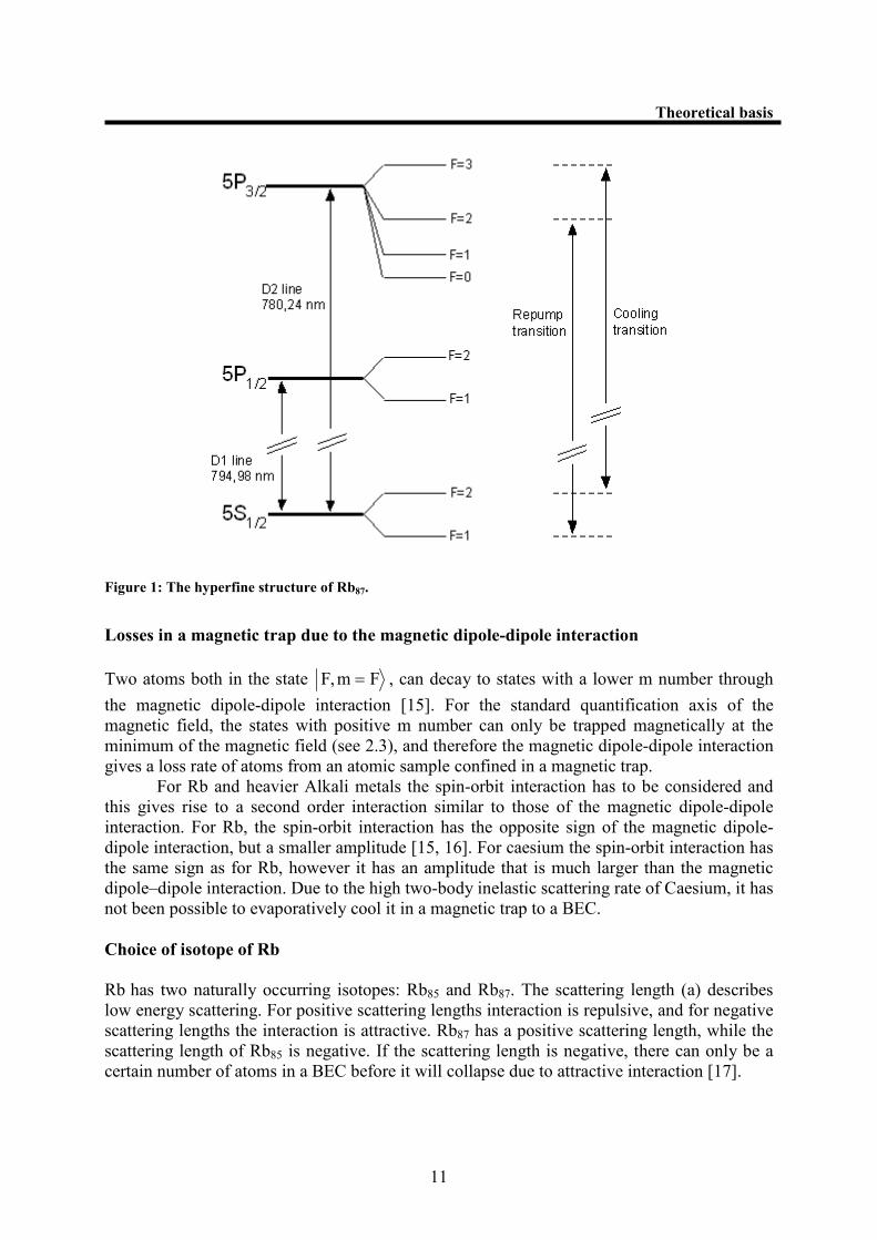
A compendium of data of Rb87 can be found in [98]. The level scheme for Rb87 can be seen in
Figure 1. The transition from the ground state 2F,S5 2/1 = to the excited state 3F,P5 2/3 =
can be approximated as a cycling transition, and it will be referred to as the cooling transition.
The frequency difference between the cooling transition and the transition from 2F,S5 2/1 =
to 2F,P5 2/3 = is 267 MHz. If the frequency of the illuminating light is resonant with the
cooling transition, then the ratio of the probability for a Rb87 to be excited to the state
3F,P5 2/3 = compared to the probability to be excited to the state 2F,P5 2/3 = is 8000, if
the saturation broadening of the atomic transitions is not considered. In the state 2F,P5 2/3 =
the atom can both decay to the state 2F,S5 2/1 = with the probability 5/8 and it can decay to
the state 1F,S5 2/1 = with the probability 3/8. In the state 1F,S5 2/1 = an atom will be far
off resonant compared to the cooling transition (6.8 GHz) and in order for the atom to be
cooled on the cooling transition again, it must be pumped back to the state 2F,S5 2/1 = . A
laser resonant on the transition from 1F,S5 2/1 = to 2F,P5 2/3 = can pump the atoms back
to the state 2F,S5 2/1 = . The fact that only one extra single laser beam is needed to pump the
atoms back to the ground state of the cooling transition is an advantage shared by all the
Alkali metals.
The wavelength of the D2 line at 780 nm is easily generated by commercially
available diode lasers. The vapour pressure of Rb at room temperature is high (melting point
39.3 °C) [98]. Due to this a Rb vapour cell at room temperature of a few cm length can
generate a good absorption signal.
Page 12
11
Theoretical basis
Figure 1: The hyperfine structure of Rb87.
Losses in a magnetic trap due to the magnetic dipole-dipole interaction
Two atoms both in the state Fm,F = , can decay to states with a lower m number through
the magnetic dipole-dipole interaction [15]. For the standard quantification axis of the
magnetic field, the states with positive m number can only be trapped magnetically at the
minimum of the magnetic field (see 2.3), and therefore the magnetic dipole-dipole interaction
gives a loss rate of atoms from an atomic sample confined in a magnetic trap.
For Rb and heavier Alkali metals the spin-orbit interaction has to be considered and
this gives rise to a second order interaction similar to those of the magnetic dipole-dipole
interaction. For Rb, the spin-orbit interaction has the opposite sign of the magnetic dipole-
dipole interaction, but a smaller amplitude [15, 16]. For caesium the spin-orbit interaction has
the same sign as for Rb, however it has an amplitude that is much larger than the magnetic
dipole–dipole interaction. Due to the high two-body inelastic scattering rate of Caesium, it has
not been possible to evaporatively cool it in a magnetic trap to a BEC.
Choice of isotope of Rb
Rb has two naturally occurring isotopes: Rb85 and Rb87. The scattering length (a) describes
low energy scattering. For positive scattering lengths interaction is repulsive, and for negative
scattering lengths the interaction is attractive. Rb87 has a positive scattering length, while the
scattering length of Rb85 is negative. If the scattering length is negative, there can only be a
certain number of atoms in a BEC before it will collapse due to attractive interaction [17].
Page 13
12
Theoretical basis
3-body recombination
For the formation of a molecule at least three atoms have to be involved in the scattering
process as one atom must carry the extra energy away. The 3-body recombination rate for
Rb87 is in [18] calculated to be a factor 50 smaller than the ones for Li7 and Na23. The atoms
in a molecule are not trapped in the magnetic trap, and thus the 3-body recombination leads to
loss at high densities.
Rb87 was chosen as the element to condensate to a BEC due to its simple level
structure, positive scattering length, a low two-body inelastic scattering rate and a low 3-body
recombination rate.
2.2 Magnetic optical trap
The magnetic optical trap (MOT) is a highly effective method of cooling and trapping
an atomic sample. In a MOT it is possible to capture up to 1010
atoms at temperatures of a
few tens of µK, and with densities up to 1012
atoms/cm3 from a room temperature background
gas. In this chapter the key concepts are introduced. A good introduction to laser cooling and
MOT theory can be found in [50].
Controlling the motion of an atom with light forces
The absorption process of a photon from a laser beam gives the atom a momentum transfer in
the propagation direction of the laser beam. Spontaneous emissions are in a random direction,
and the net momentum transfer averaged over many spontaneous emissions is zero. Hence,
the absorptions from a laser beam and spontaneous emissions give a directional momentum
transfer over time. This force on an atom can be used to control the motion of an atom.
Magnetic optical trap (MOT)
A three dimensional MOT consists of three pairs of counter propagating laser beams. The 3
pairs of laser beams are red-detuned to an atomic resonance, and their propagation directions
are perpendicular to each other. An atom moving in a direction opposite to the propagation
direction of one of the six laser beams will be more resonant with that laser beam than the
others. This is the well known Doppler Effect. As the atom is more likely to absorb photons
from the laser beams propagating in the opposite direction of its velocity, the net momentum
transfer due to absorptions from the laser beams will be in the opposite direction of the
velocity of the atom. In other words the absorption processes act as a friction force on the
atom.
By adding a magnetic field gradient the energy of Zeeman levels become position
dependent, and this position dependency combined with a particular polarization of the 6 laser
beams can be used to create a confining potential for an atom. The resonant photons emitted
by the atoms captured in the MOT creates an internal pressure, and this limits the maximum
obtainable density to ~1012
atoms/cm3 [19,20]. An atomic sample held in a MOT with a
density limited by the internal light pressure is said to be in the density limited regime.
Page 14
13
Theoretical basis
The Doppler temperature
The illuminating light also heats the atoms through random recoils, and the steady state
temperature expected is the Doppler temperature. The temperature corresponding to one
recoil created by a spontaneous emission of a photon is the minimum obtainable temperature,
and it is known as the recoil temperature.
Sub-Doppler cooling
It is possible to cool to substantially lower temperatures than the ones indicated by the
Doppler temperature. This is known as sub-Doppler cooling, and the type of sub-Doppler
cooling used in this experiment is known as σ +, σ
- polarization gradient cooling [21]. This
type of cooling relies on the different transition probabilities between the different Zeeman
levels and to enable this type of cooling the Zeeman levels have to be degenerate.
Therefore, it is often advantageous to have a short period of σ +, σ
- polarization
gradient cooling after a sufficient number of atoms have been captured in the MOT to
increase the phase space density. The magnetic field is quickly switched off and the laser
beams are further detuned. The practical implementation of this step is described in chapter
5.3.
2.3 Magnetic traps
The phase space density of an atomic sample in a MOT is typically a factor 10
6 lower
than the phase space density needed to reach the transition to BEC. For the last step the
atomic sample can be transferred to a magnetic trap or dipole trap for evaporative cooling.
The advantage of a magnetic trap compared to a dipole trap is that in a magnetic trap forced
evaporation can be used without changing the confinement for the atoms that remain in the
trap. The disadvantage of capturing the atoms in a magnetic trap compared to a dipole trap is
the losses due to inelastic collisions and 3-body recombination, which do not occur in a dipole
trap.
Magnetic trapping of neutral atoms
The potential energy of a neutral atom in a magnetic field is given by:
)r(Bµ)rU(rrvr
⋅−= (1)
where µv
is the magnetic moment of the atom and )r(Brr
is the B-field. The energy shift
of the states m,2/1J,2/3I,2F === due to an external magnetic field can be calculated
according to the Breit-Rabi formula in the limit where the energy shift due to the magnetic
field is small compared to the hyperfine splitting [22,98]:
2Fhfs
FBFFm,I,2/1J,2F x1I2
xm41
2
EBmgE +
++
∆+µ=∆ == (2)
Page 15
14
Theoretical basis
where hfsE∆ is the hyperfine splitting, hfs
BIj
E
B)gg(x
∆
µ−= , gI is the g-factor for the
nucleus, gJ is the g-factor for the electron, gF is the Lande factor and mF is an integer from – 2
to +2. The quantification axis for the m states is in the direction of the magnetic field. The
values for the g-factors for Rb87 can be found in [98]. At a low magnetic field the second term
in equation 2 is much smaller than the first term and in this case the potential seen by the
atoms in the ground state F2/1 m,2F,S5 = is:
)r(Bmg)r(U FBF
rrµ= (3)
Depending on the sign of gF, the states with positive m number will either experience a
force towards low field (low field seeker) or high magnetic field (high field seeker). In [23] it
is proven that no magnetic maximum can exist in free space, and thus only low field seeker
states can be captured in an inhomogeneous magnetic field.
Majorana spin flips
It is possible for an atom in a given Zeeman level to undergo a non-adiabatic crossing into
another Zeeman level. The smaller the energy gab between the two levels is, the larger the
probability is for a non-adiabatic crossing to occur is. This type of non-adiabatic crossing is
known as Majorana spin flips. The probability for a non-adiabatic crossing at the minimum
energy difference can be estimated as lzePΓ−= π2
where Γlz is the Laundau-Zener parameter
and it is given by [24,25]:
vBm
Bg
dt
dE
E
F
BFlz
'44
2
min
2
min
hh
µ≈
∆=Γ (4)
where Bmin is the magnetic field at the minimum of the trapping region. dt
dE can be
estimated as: vBdt
dr
dr
dE
dt
dE'≈= , where 'B is the gradient of the magnetic field and v is the
velocity of the atom. For Γlz >> 1 the probability for an atom to undergo a non-adiabatic
crossing to an other Zeeman state is small.
The life time associated with Majorana spin flips (τ0) in a linear trap r'B)r(Brr
= only
depends on the width of the atomic sample, and it is given by [26]:
)(s/mm4
10 3,77 τ 2
22
FWHM0 σ= , where σFWHM is the full width half maximum of the atomic
sample.
Page 16
15
Theoretical basis
0 0.2 0.4 0.6 0.8 10
20
40
60
80
sFWHM Hmm L
t 0HsL
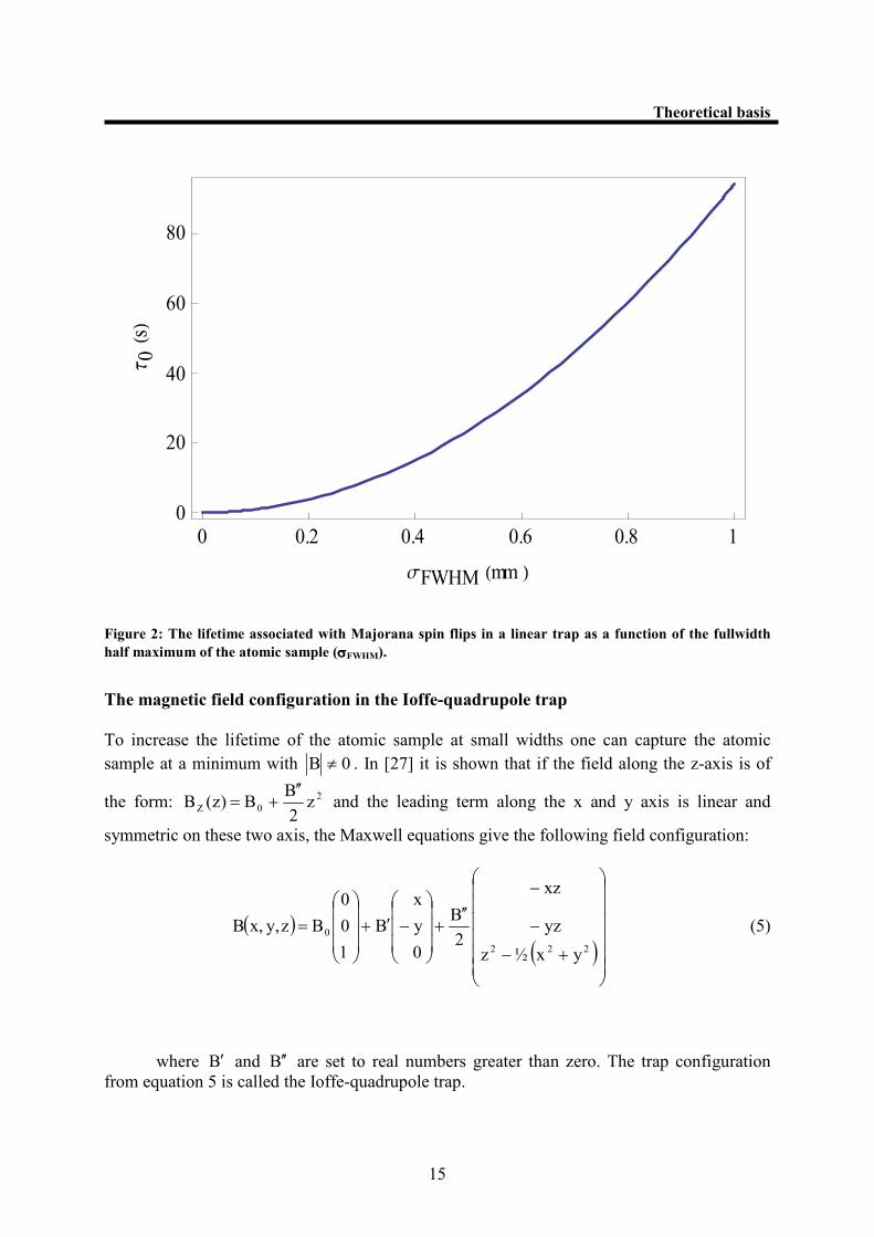
Figure 2: The lifetime associated with Majorana spin flips in a linear trap as a function of the fullwidth
half maximum of the atomic sample (σσσσFWHM).
The magnetic field configuration in the Ioffe-quadrupole trap
To increase the lifetime of the atomic sample at small widths one can capture the atomic
sample at a minimum with 0B ≠ . In [27] it is shown that if the field along the z-axis is of
the form: 2
0Z z2
BB)z(B
′′+= and the leading term along the x and y axis is linear and
symmetric on these two axis, the Maxwell equations give the following field configuration:
( )( )
+−
−
−
′′+
−′+
=222
0
yx ½z
yz
xz
2
B
0
y
x
B
1
0
0
Bzy,x,B (5)
where B′ and B ′′ are set to real numbers greater than zero. The trap configuration
from equation 5 is called the Ioffe-quadrupole trap.
Page 17
16
Theoretical basis
For B/Byxρ 0
22 ′<<+= the amplitude of the magnetic field can be approximated
with [10]:
( ) 0
22
radial BzBB2
1)z,(B +′′+ρ′′=ρ (6)
where 2
B
B
BB
0
2
radial
′′−
′=′′ . A displacement along the z-axis term xz
2
B ′′−destructively
interfere with the term x'B and this lowers the radial confinement along the x-axis. The point
on the z-axis (Zno trap) with no confinement on the x-axis is [10]:
′
−′′′
±=B2
B
B
BZ 0
trapno (7)
Zno trap limits the size of an atomic sample, which can be captured in the magnetic trap
given by equation 5. For a negative B0 there exist two minima with B = 0. For B0 approaching
zero the two minima move towards each other and coincide at B0 = 0. For B0 greater than zero
there is an local minima with a B-field greater than zero on the z-axis. In chapter 5.5 it is
explained, how to generate a field configuration that closely resembles the one given in
equation 5.
Adiabatic heating due to compression
The volume occupied by an atomic sample depends on the trap geometry. A generalized
trapping potential can be written as:
zyx s
z
z
s
y
y
s
x
xa
z
a
y
a
x)z,y,x(U ε+ε+ε= (8)
In [28] it is proven that the volume scales with the temperature as ξT~V , where
zyx s
1
s
1
s
1++=ξ . The linear trap has ξ = 3, the harmonic trap has ξ = 3/2 and the Ioffe-
quadrupole trap at high temperatures ( )0BB BTk µ>> has ξ = 5/2.
If an atomic sample is compressed or expanded adiabatically (no energy transfer in the
process), the phase space density of the atomic sample does not change. The phase space
density (ϖ) is defined as the number of atoms inside a cube with the length equal to the de
Broglie wavelength, and it is given by [15]:
2/3
B
2
Tmk
2n
π=ϖ
h (9)
Page 18
17
Theoretical basis
From equation 8 it follows that if the potential U is changed with a factor β, the volume for a
fixed temperature is changed with a factor β-ξ if the atoms are assumed not to interact (ideal
gas). From the assumption of an adiabatic compression the temperature change and the
density change are respectively: ξ+
ξ
β 23
2
and ξ+
ξ
β 23
4
[10]. The criterion for adiabaticity is:
2
trap
trap
dt
dω<<
ω.
2.4 Evaporative cooling
The principle in evaporative cooling is that atoms, which have a higher kinetic energy
than the average kinetic energy in the atomic sample, are removed. After having lost a group
of relative hot atoms, the remaining atoms will rethermalize to a lower temperature after some
time due to collisions between the atoms. Good introductions to evaporative cooling can be
found in [29,30].
The parameter αααα describing the efficiency of evaporative cooling
The average energy of the remaining atoms can be estimate from [15]:
dNN
dN)1(Ed
+εα++
=ε+ε (10)
where ε is the average energy of an atom before evaporation, εd is the energy change
due to evaporation, E is the energy of the entire atomic sample before evaporation, N is the
number of atoms in the atomic sample before evaporation, dN is the number of atoms lost in
the evaporation (dN < 0) and εα+ )1( is the average energy of the atoms removed in the
evaporation. By assuming that dN and dε are small compared to respectively N and ε ,
equation 10 can be approximated as:
α=ε
)Nln(d
)ln(d (11)
According to the Virial theorem, the average kinetic energy of an atom held in a power
law potential is proportional to the average potential energy. Due to this ε can be substituted
with the temperature T in equation 11.
α=)Nln(d
)Tln(d (12)
If α is independent of N, the relation between T and N is:
α
=
00 N
N
T
T where T0 is
the temperature, and N0 is the atom number before evaporation. α is a good figure of merit to
describe how effective a given evaporation run has been.
Page 19
18
Theoretical basis
In [30] it is calculated how the different thermodynamic variables relevant for
evaporation cooling scales compared to N and α.
The thermodynamic variable X scales as:
q
00 N
N
X
X
= and the exponent q is given in
Table 1.
Thermodynamic variable (X) q
N 1
T α
Volume ξα
Density 1-ξα
Phase space density 1-α(ξ+3/2)
Collision rate 1-α(ξ-1/2)
Table 1: Evaporation parameters dependence on the atom number [30].
If the exponent q is larger than one for the collision rate, the number of collisions
increases during the evaporation, which is called runaway evaporation. From Table 1 it is
clear that a high value of ξ is desirable as it gives a greater increase in phase space density for
a fixed α and atom loss. For this reason a linear trap is a very suitable trap for evaporation as
long as losses due to Majorana spin flips are not important.
Simple model for evaporative cooling
In a simple model of evaporative cooling one can assume that all atoms with energies above a
certain limit Ui are removed instantly from the trap. Collisions between the atoms remaining
in the trap redistribute energy and create atoms with energies above Ui. The probability for an
atom to acquire an energy above Ui through collisions depends on the temperature of the
atomic sample in a given potential. By calculating the time for the number of collisions for
the sample to thermalize, and the fraction above Ui for a thermalized sample, the number of
atoms removed due to acquiring energies above Ui from collisions can be estimated. An
average of 2.7 collisions are needed for thermalization [31]. The fraction above Ui for a
thermalized sample with the temperature T is: Tk
U
B
i
e1−
− .
By choosing Ui a compromise has to be found between the cooling rate and the
average energy of the atoms removed from the trap. If only the atoms can escape the trap by
obtaining energies larger than Ui through collisions, a high Ui compared to kBT means a high
α but a low cooling rate.
An atomic sample held in a magnetic trap has a certain lifetime associated with other
loss processes than the one used for evaporation. Collisions with a background gas, inelastic
collisions and 3-body recombinations are among the loss processes, which limit the lifetime
of an atomic sample in a magnetic trap. The average energy of the atoms removed by these
loss processes affects the value of α. By assuming that all other loss processes than the one
Page 20
19
Theoretical basis
used for evaporation can be described by a lifetime independent of N and T (τloss) and
assuming all evaporated atoms have the energy Ui, an expression for α can be written [15]:
Tk
U
i
B
loss
el
B
i
B
i
eU
Tk21
1Tk)2/3(
U
τ
τ+
−ξ+
=α (13)
where τel is the collisions time for elastic collisions and it is given by:
relcol
el
v)0(nt
1σ= (14)
where n(0) is the density in the centre of the trap, σcol is the collision cross section and
vrel is the mean relative velocity of the atoms in the atomic sample m
Tk4 B
π[15]. If the
temperature of the atoms is low enough for the scattering to be assumed to be pure s-wave
scattering, then: σcol = 8πa2. The maximum value of α for a given ratio of (τloss /τel) for a
linear trap (ξ=3) is plotted in Figure 3.
The run-away regime for a linear magnetic trap
For a trap with ξ = 3, α must be greater than 2/5 for collision rate not to decrease during the
evaporation according to Table 1 (the runaway regime). According to Figure 3 this means the
collision time between the atoms have to be a factor 1500 shorter than the lifetime of the
atomic sample. In [14] a ratio of 100 between the collision rate and the loss rate is suggested
as a rule of thumb as a condition for runaway evaporation.
Typical values for an sample transferred from a MOT to a magnetic trap are of the
order: n(0) = 1011
atoms/cm3, T = 100 µK and scattering lengths for the ground states of Rb87
are around 100 a0 [15,32]. a0 is the Bohr radius. This gives a value of τel ≈ 50 ms and this
means the lifetime of the atomic sample in the trap have to be greater than 75 s for the
evaporation to be in the run away regime in a trap with ξ = 3.
Forced evaporation with a radio frequency field
In a magnetic trap the low field seeking states can be removed from the trap by inducing
transitions into untrapped states. This can be done by an oscillating magnetic field with a
frequency ψ0. The spin of a photon is h , and thus a scattering event of one radio frequency
photon can change the m-number of a trapped atom by 1. The probability for such a transition
is largest, if the energy of the radio frequency photon is equal to the energy difference
between two adjacent Zeeman levels (∆m=1).
Page 21
20
Theoretical basis
0 2000 4000 6000 8000 10000
0
0.2
0.4
0.6
0.8
tloss êtel
a
Figure 3: The maximum value of αααα for a given ratio of (ττττloss /ττττel) for a linear trap (ξξξξ=3).
The potential energy of the atoms where the transition probability is the largest to an
adjacent Zeeman level, is:
0FB0i BgU µ−Ψ= h (15)
Hence, by varying ψ0 one can selectively remove atoms with a certain potential
energy. The orbit of an atom with a higher total energy than Ui has some probability to cross
the region, where the potential energy is Ui. If this probability is high, the trap is said to have
“sufficient” ergodicity and the assumption that all atoms with total energies above Ui will be
removed is good. Collisions between the atoms in the trap change the orbits of the atoms, and
this typically ensures the criterion for “sufficient” ergodicity. In [33] the effect of non-
ergodicity is discussed.
A second assumption is that atoms with energies above Ui are instantly removed from
the trap. This is a good assumption if the removed atoms do not collide with atoms remaining
in the trap. A necessary condition for this is that the collisional free path length of an atom in
the gas is much longer than the length of the sample (the Knudsen regime).
A limiting factor in evaporative cooling is incomplete evaporation due to the quadratic
Zeeman term (see equation 2). Due to the quadratic Zeeman term the energy difference
between two adjacent Zeeman levels is no longer independent of m and an atom in the state
with m = 2 cannot therefore any longer at same position cascade down to an untrapped state at
the same position at a fixed radio frequency. This effect becomes important at magnetic fields
around 20 Gauss, and it is discussed in [34,35].
Page 22
21
Theoretical basis
Losses in a magnetic trap due to 3-body recombination of Rb87
At high densities tree-body recombination losses become important and the lifetime
associated with 3 body losses scales as:
2
body3
Ln1
−=τ
(16)
In [36] the 3-body recombination rate (L) for Rb87 is measured to be 4.3 10-29
cm6/s
for a thermal gas. The 3 body recombination rate is a factor six times lower for a pure
condensate [15,36].
The phase density of an atomic sample close to the transition temperature to BEC is
close to one. Assuming the transition temperature is 500 nK, the density of the atomic sample
at the transition is 5 1013
atoms/cm3 and the lifetime associated with 3-body losses is then 10
sec.
2.5 A dilute Bose gas in a harmonic potential
The general form of the atomic distribution depends on the potential and the
temperature of the atomic sample. At temperatures where the kinetic energy is much larger
than the energy due to interaction between the atoms, the atomic sample can be treated as an
ideal gas (no interaction). This approximation is typically good for an atomic sample with a
temperature much larger than the transition temperature for a BEC for the atomic sample (a
thermal cloud). At low enough temperature the interaction energy becomes much larger than
the kinetic energy, and the kinetic energy can be neglected.
This approximation is typically good for a pure BEC, and it is known as the Thomas-
Fermi approximation. It is relative simple to find the atomic distribution with the ideal gas or
the Thomas-Fermi approximation. It is, however, not simple to solve the atomic distribution
around the transition temperature to a BEC (tc). A simple way to describe the atomic
distribution around tc is to assume that the atomic sample consists of two separate samples: a
pure BEC and a thermal cloud.
The spatial distribution of a thermal atomic cloud in a power law potential
The occupation number kn for a Bose-distribution is at the temperature T:
∑∞
=
µ−ε−
µ−ε=
−
=1l
Tk
)(l
Tk
kB
k
B
k
e
1e
1n (17)
where εk is the energy of the energy level k and µ is the chemical potential. The
chemical potential is decided through the atom number N:
∑=k
knN (18)
Page 23
22
Theoretical basis
If the level spacing between the energy levels in the magnetic trap is much smaller than kBT,
the number of atoms in the excited state can be written as:
εερ
−
=− ∫∞
µ−εd)(
1e
1NN
0 Tk
0
B
k
(19)
where N0 is the number of atoms in the ground state, ρ(ε) is the density of states, and it
is given by [28]:
∫ε
−επ
=ερV
3
3
2/3
dr)r(Uh
)M2(2)( (20)
where Vε is the volume, where r fulfils the following condition: ε - U(r) ≥ 0. The
density of the atoms in the excited states in a power law trap is [28]:
))r(z(g1
)r(n 2/33
dB
th λ= (21)
where Tk
U(r)µ
Be z(r)
−
= and the Bose function is: ( ) ∑∞
=
=1i
j
i
ji
zzg . For a thermal cloud in
the Ioffe-quadrupole trap at low temperatures (kBT<< B0µB) the trap is harmonic
( )22
z
22
y
22
x zyxm2
1)r(U ω+ω+ω= (see chapter 2.2).
The spatial distribution of a freely expanding thermal cloud
The density profile during a free expansion of an atomic sample, which has been captured in a
harmonic potential is given by [10]:
∑
+ωλ=
+ω
ω−µ
=
=∏)Tk/(
1tq
2
m
2/3
z,y,xq22
q
3
dB
tof
B
z,y,xq22
q
2q2
eg1t
11)t,r(n (22)
If Z << 1 the following approximation can be made for the Bose function g3/2(Z) ≈ Z.
In the classical limit µ << 0, and the density can be approximated as:
∑
π
−≈ =
=∏
z,y,xq
2
e/1 )t(q
q
z,y,xq
e/1
2/3
0
tof e)t(q
NN)t,r(n (23)
where q1/e(t) is the 1/e radius and it is given by:
Page 24
23
Theoretical basis
2
0
22
2
q
B2B
e/1 qtvm
Tk2t
m
Tk2)t(q +=
ω+= (24)
where v is the velocity and q0 is the 1/e radius at t = 0 of the atomic sample. The
expansion of an atomic sample released from a non-harmonic potential is different from
equation 24, however for expansions times, where the atomic sample has expanded to a size
significantly larger than the original size, the expansion behaviour described by equation 24 is
typically a good approximation.
The spatial distribution of a pure BEC with the Thomas-Fermi distribution
For a pure BEC, all atoms are in the same single-particle state and the many body
particle function of the entire sample ψ(r) is simply a product of the same single particle wave
function. ψ(r) is described by the Gross-Pitaevskii equation. An introduction for the solutions
of the Gross-Pitaevskii equation for trapped bosons can be found in [15,37]. The Gross-
Pitaevskii equation is:
2
0
22
)r(U)r()r(U)r(m2dt
)r(di ψ+ψ+ψ∇−=
ψ hh (25)
where U0 is the interaction energy due to two-body collisions ( )m/a4U 2
0 hπ= . The
interaction term ( )2
0 )r(U ψ can be identified as the chemical potential (µ).
In the Thomas-Fermi approximation the kinetic energy term is set to zero and the
steady state distribution becomes [10]:
z)y,x,(q q qfor z
z
y
y
x
x1
zyx
N
8π
15(r)n 0
2
0
2
0
2
0000
0
TF =≤
−
−
−= (26)
where 2
q
0m
2q
ω
µ= and q = (x,y,z). For 0(r)n q q TF0 => . The Thomas-Fermi
approach is applicable when ψ(r) varies slowly in space. For large BECs this is typically the
case, but near the surface of the BEC the Thomas-Fermi approximation fails.
The spatial distribution of a freely expanding BEC
The expansion of the cloud from a cigar-shaped trap (ωρ = ωx = ωy >> ωz) is [38]:
22
0 t1)t( ρω+ρ=ρ (27)
Page 25
24
Theoretical basis
( ) ( ) ( )
+−+= ρρρ
2
ρ
z
z
ρ
0 tω1lntωArcTantωω
ω
ω
ωρz(t) (28)
The atomic distribution of a partly condensed cloud can be approximated by a
distribution for the BEC with N0 atoms given by equation 26, and a thermal cloud with N-N0
atoms given by equation 21. The resulting atomic distribution is bimodal and the bimodality
can be observed in the atomic distribution after a sufficient time of expansion depending on
the trap parameters. Bimodality of the atomic distribution is a clear proof of a BEC.
It is possible for a non-condensed cloud to be in the regime where the Thomas-Fermi
approach is valid. A necessary condition for the Thomas-Fermi approximation to be valid is:
nm
a4)r(UTk
2
3E
22
0Bkin
hπ=ψ<<= (29)
If the phase density is assumed to be 1, the temperature has to be greater than 300 µK
for equation 29 to be valid. Then the density is then of the order 1017
atoms/cm3. Such an
atomic sample cannot be experimentally realized with the present apparatus. A BEC has a
phase space density of typically 107, and thus the temperatures and densities, at which
equation 29 is valid, are much lower than for a non-condensed cloud. In practice, if an atomic
sample has an expansion following equation 27 and equation 28, it can be taken as a clear
proof of a BEC.
The column density of thermal cloud and a BEC
The column density along an imaging axis is much easier to measure directly than the density.
Defining the imaging axis to be the y-axis and integrating the atomic distributions from y = -
∞ to y = ∞, column densities for a thermal gas and a Bose-Einstein condensate are [10]: 2
0,th
2
0,th
2
0,th
2
0,th z
z
x
x1
th
z
z
x
x1
2
2
thth e)0(n~eg
)1(g
)0(n~)z,x(n~
−
−
−
−
≈
= (30)
z)x,(q q qfor z
z
x
x1(0)n~z)(x,n~ TF,0
2
TF,0
2
TF,0
TFTF =<
−
−= (31)
where )0(n~ th and )0(n~TF are the column densities respectively for a thermal gas and
for a gas in the Thomas-Fermi limit at x = z = 0. 00,TFx ρ= and z
ρ
00,TFω
ωz ρ= .
Page 26
25
Theoretical basis
2.6 Absorption imaging
The only feasible method to measure the density distribution of an atomic gas with up
to 1010
atoms is with optical methods. The simplest method to imagine the atomic sample is
by illuminating it with light, and measure the absorption as a function of the displacement
from the centre of the sample. From this method, the column density of the sample can be
measured. By comparing the light intensity with and without atoms on a CCD chip, the
optical density can be estimated. Among the systematic errors in this measurement is the dark
signal on the CCD chip, the saturation effect of the illuminating light on the atomic sample,
the resolution of the CCD chip, off-resonant light and scattering light on the CCD chip due to
absorption of the illuminating light from the atomic sample. By accounting for these errors a
measure for the column density can be found and the temperature can be estimated by
measuring the column density at various expansion times (Time of flight (TOF)).
Beer’s law
For the absorption imaging a laser beam is used as the spectrum is close to monochromatic,
and it has a well-defined propagation direction. The optical density (OD) of an atomic sample
at a given position in the plane perpendicular to the propagation direction of the laser beam is
defined by Beer’s law, and it is given by:
OD
0 e)z,x(I)z,x(I −= (32)
where I(x,z) is the intensity on the CCD chip if the laser beam had passed through an
atomic sample, and I0(x,z) is the intensity on the CCD chip in the absence of an atomic
sample.
The measured optical density
The measured value for the optical density is given by:
−
−=
dark
dark0
measureII
IIlnOD (33)
where Idark is the intensity measured on the CCD chip in the absence of any
illuminating light (the dark signal).
Correction factors for the measured optical density
The resolution of the CCD chip and the scattered light due to absorption set an upper
limit on the maximum measurable optical density (ODsat). The correction for optical density
due to a maximum measurable optical density is given by [14]:
satmeasure
sat
ODOD
OD
modee
e1lnOD
−−
−
−
−= (34)
Page 27
26
Theoretical basis
To obtain the most reliable value of the optical density it is preferable that
ODmeasure< ODsat/2, so that the correction factor is not big. The illuminating light saturates the
atoms and this lowers the measure absorption.
The actual OD can be estimated from [14]:
( )S
OD
modactualI
Ie1ODOD mod−−+= (35)
where IS is the saturation intensity. In the limit of no saturation the optical density is
given by [10]:
20
21
1)z,x(n~)z,x(OD
γδ
+
σ= (36)
where n~ is the column density, σ0 is the absorption cross section and γ is the natural
linewidth of the imaging transition.
Page 28
27
Cavity theory
3 Cavity theory
In this chapter a review of the important concepts needed to understand the next
chapter regarding cavity/atom interaction. In [39] an introduction to the classical theory of
Gaussian beams and cavities are given. Chapter 3.1 gives the characteristics of Gaussian
beams. Chapters 3.2 to 3.4 describe how one can most optimal couple light into a high finesse
cavity. Chapter 3.5 discusses how a cavity can change the emission spectrum of an atom.
3.1 Gaussian beams
A Gaussian beam is a good approximation for the beam generated by a laser. The
electrical field of a Gaussian beam is given by equation 37 [39].
tiw(z)
yx
2R(z)
yxik
)(z/ztani(kz0 eeeew(z)
wat)z,y,E(x,
2
2222
01 ω
=
+−+
− −
(37)
2
0
2
0z
z1ww(z) += (38)
z
zzR(z)
2
0+= (39)
where E(x,y,z,t) is the electrical field of the beam at the position (x,y,z) and at the time
t, 2
0w
P2a
π= , P is the power of the Gaussian beam, z0 is the Rayleigh range, k is the wave
number (2π/λ), λ is the wavelength of the light, w0 is the waist of the laser beam at the focus,
w(z) is the waist at the position z and R(z) is the radius of curvature of the laser beam at the
position z. The Rayleigh length and the waist w0 have the following relation [39]:
λ
wπz
2
00 = (40)
Figure 4: A Gaussian beam along its axis of propagation.
Page 29
28
Cavity theory
The Gaussian beam as described by equation 37 is a TEM00 mode. The TEMmn mode
has m zero crossings on the x-axis and n zero crossings on the y-axis.
3.2 Cavity stability
The cavities described in this thesis are all standing wave cavities. For the photons
inside the cavity to have a high storage time, the cavity must be stable.
Figure 5: The arrow shows a stable path for a light ray inside a spherical resonator. The beam is reflected
upon itself on each of the two mirrors and thus can stay an infinite number of reflections inside the
resonator, if it is not transmitted through or scattered on the mirrors.
That a cavity is stable means that it is possible for a light ray originating anywhere on
the surface of one of the mirrors to stay inside the cavity for an infinite number of reflections
on the two mirrors.
Ray optics
The constraints on the radius of curvature of the two mirrors and the length of the cavity for it
to be stable can be calculated with ray optics. In ray optics, a ray is described by a 2-
dimensional column vector
=
'r
rrr
where r is the lateral displacement and r’ is the angle (see
Figure 6).
Each optical element is described by a 2x2 matrix. Ray matrix for a spherical mirror is
given by M1 and free propagation is given by M2. R is the curvature of the mirror and d is the
distance travelled by the ray [39].
=
1R2-
01
1M
=
10
d1
2M
To calculate the new vector for a ray after an optical element, the relevant matrix is
multiplied with the vector for the ray ( )rMr. For an optical system consisting of more than one
element, the matrixes for the different elements can be multiplied together to create one
matrix for the entire system. The resulting matrix is of the type:
DC
BA and is called an
ABCD matrix.
Page 30
29
Cavity theory
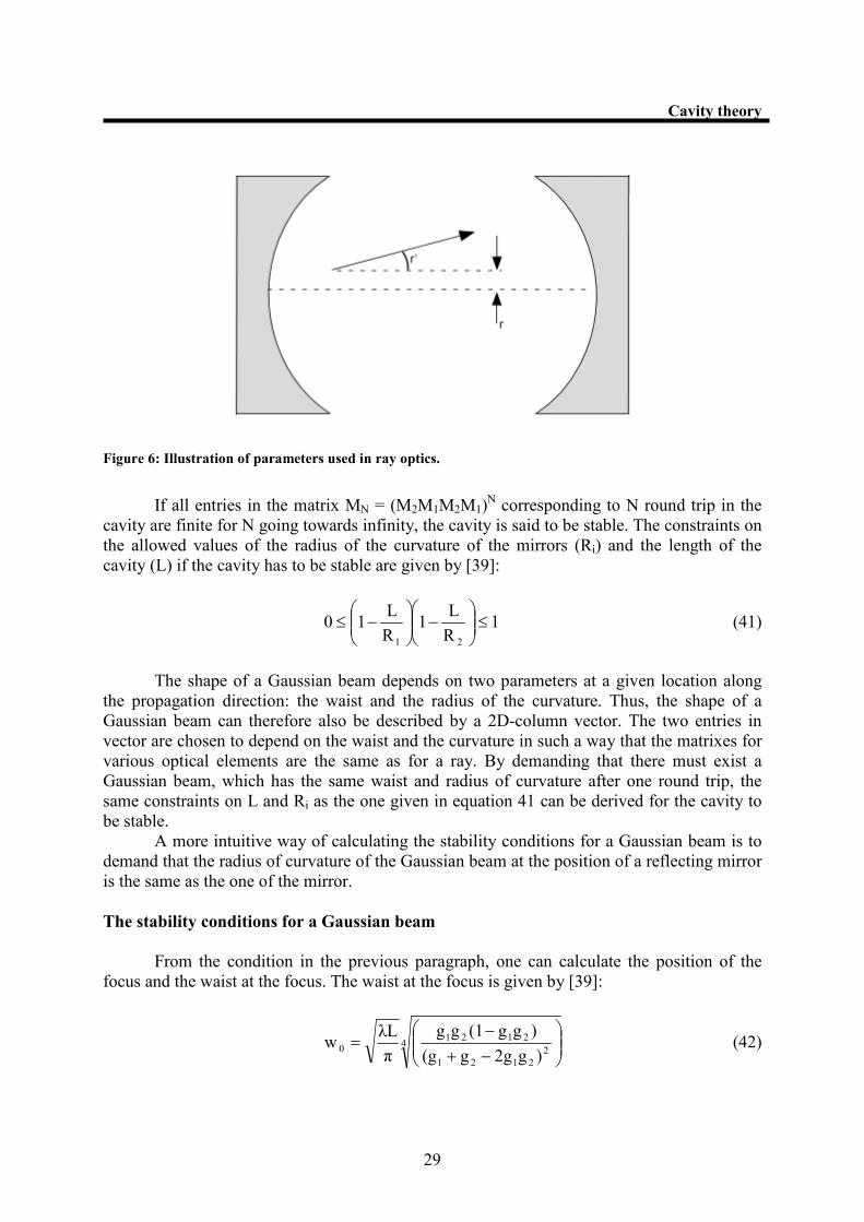
Figure 6: Illustration of parameters used in ray optics.
If all entries in the matrix MN = (M2M1M2M1)N corresponding to N round trip in the
cavity are finite for N going towards infinity, the cavity is said to be stable. The constraints on
the allowed values of the radius of the curvature of the mirrors (Ri) and the length of the
cavity (L) if the cavity has to be stable are given by [39]:
1R
L1
R
L10
21
≤
−
−≤ (41)
The shape of a Gaussian beam depends on two parameters at a given location along
the propagation direction: the waist and the radius of the curvature. Thus, the shape of a
Gaussian beam can therefore also be described by a 2D-column vector. The two entries in
vector are chosen to depend on the waist and the curvature in such a way that the matrixes for
various optical elements are the same as for a ray. By demanding that there must exist a
Gaussian beam, which has the same waist and radius of curvature after one round trip, the
same constraints on L and Ri as the one given in equation 41 can be derived for the cavity to
be stable.
A more intuitive way of calculating the stability conditions for a Gaussian beam is to
demand that the radius of curvature of the Gaussian beam at the position of a reflecting mirror
is the same as the one of the mirror.
The stability conditions for a Gaussian beam
From the condition in the previous paragraph, one can calculate the position of the
focus and the waist at the focus. The waist at the focus is given by [39]:
42
2121
21210
)g2gg(g
)gg(1gg
π
λLw
−+
−= (42)
Page 31
30
Cavity theory
where gi = 1-L/Ri. The Rayleigh length corresponding to the waist given by equation
42 can be calculated from equation 40. For a cavity consisting of two identical mirrors, the
focus is at the centre of the cavity (equal distance to both mirrors).
If a Gaussian beam has the same phase after one round trip, it will constructively
interfere with itself. This is fulfilled for the following frequencies [39].
( )
+= −21
1
q ggcosπ
1q
2L
cf (43)
where c is the speed of light, q is a natural number, and q gives the frequencies of the
longitudinal modes of the cavity. FSR = c/(2L) is the free spectral range, and it is the
frequency difference between two longitudinal modes. If a Gaussian beam fulfils the
constraint in equation 43, the beam is said to be resonant with the cavity.
3.3 Cavity incoupling
This chapter is describing, how to couple light into a cavity through one of the mirrors.
The mirror consists of a plane side of glass without a coating, which has a few percent
reflection and a curved side with a highly reflecting coating. The reflection from the plan side
is neglected due to its much higher transmission than the coated side. In the following
discussion a Gaussian beam that fulfils the conditions for being a stable mode of the cavity is
considered.
Figure 7: illustration of different electrical field arising when a laser beam is sent to the incoupling mirror
of a cavity.
One part of the incoming Gaussian beam will be directly reflected at the mirror coating
of the incoupling mirror, and the other part of the beam is transmitted into the cavity. A part
of the beam, which was transmitted into the cavity, will be transmitted through the incoupling
mirror after one round trip in the cavity. This beam will have the same parameters as the
directly reflected beam except for the phase. The beam, which has made one roundtrip in the
cavity, has the same phase as the incoming beam, while the phase of the directly reflected
beam has obtained a phase of p in the reflection. Hence, the beam transmitted through the
Page 32
31
Cavity theory
incoupling mirror by the light inside the cavity and the directly reflected beam destructively
interfere. This is seen as a reduction of the intensity of the light reflected by the cavity. At the
incoupling mirror, there are only two options: either the light is reflected or transmitted
through the incoupling mirror. Thus a reduction in the reflected light must mean an increase
in the light transmitted into the cavity.
The minimum ratio of the intensity of the reflected light to the intensity of the
incoming light is given by [40]:
2
021
21
IN
R
)(
41
I
I
χ+χ+χ
χχ−= (44)
where χ1 is the transmission coefficient of the incoupling mirror, χ2 is the transmission
coefficient of the second mirror, χ0 is the sum of loss processes not including the transmission
losses through the two mirrors (for a cavity in vacuum χ0 is the sum of the absorption losses
and the diffuse scattering losses on the two mirrors), IR is the reflected intensity and IIN is the
incoming intensity on the incoupling mirror. The light of the incoming beam is assumed to be
resonant with the cavity and equation 44 is only valid in the limit, where χ0, χ1, χ2 << 1 (low
loss cavity). If 201 χ+χ=χ the reflected intensity has its minimum. In this case the cavity is
said to be impedance matched. From equation 44 one can calculate the maximum possible
incoupling for a given cavity.
In an experiment the incoming beam will to some degree deviate from the
TEM00 mode of the cavity. In this case the incoming beam will be a superposition of TEM00
and higher order Gaussian modes of the cavity [41]. The higher order Gaussian modes will
usually not fulfil the phase condition, that they have the same phase as incoming beam at the
incoupling mirror after one round trip in the cavity, at the same frequency as the TEM00 mode
has. Modes that do not fulfil the frequency conditions will be directly reflected, and this is
seen as less incoupling. The maximum incoupling in a cavity is a measure for how good the
incoming beam matches the TEM00 mode of the cavity, and how well the cavity is impedance
matched.
Page 33
32
Cavity theory
3.4 Cavity enhancement
In the previous chapter it was shown that it is possible to transmit a significant part of
a Gaussian beam into a resonator mode assuming that the Gaussian beam has the right
parameters for the cavity in question. For ultra low internal losses, the intensity of the light
cycling in the cavity is much larger than the intensity of the incoming beam.
The intensity of the electrical field inside the cavity compared to the intensity of the
incoming beam on resonance and for a low loss cavity can be estimated from [40]:
A)(
4
I
I
2
021
1
IN
cavity =χ+χ+χ
χ= (45)
When the cavity is impedance matched the enhancement is 1/χ1. The transmission
through the cavity as a function of the frequency (ω) is given by [40]:
+
=
2FSR
ωSin
π
2F1
T
) (ωI
) (ωI
2
2
Max
IN
T (46)
where IT(ω) is the transmitted intensity for a Gaussian beam with the frequency (ω),
Tmax is transmission on resonance, FSR is the free spectral range and F is the finesse of the
cavity. The finesse is defined as:
2
1
T
2F
FSRI
Max
T
≡
(47)
The line width of the cavity (∆ν) is defined as the full width half maximum of the
resonance profile (∆ν=FSR/F). The finesse can also be expressed in terms of the internal
losses [40]:
021
2πF
χχχ ++= (48)
Equation 48 shows that for low losses the finesse is high and this in turn means a small
line width. When a photon can undergo many round trips in the cavity before it escapes from
the cavity, the phase it can pick up per round trip must also be small in order for it to
constructively interfere with the incoming beam. The total losses per round in the cavity can
be measured by switching the incoming beam off and the light inside the cavity will then
decay exponentially with the time constant: ( )021c
2LT χ+χ+χ= .
Page 34
33
Cavity theory
3.5 Scattering enhancement
The fact, that an optical resonator can change the spontaneous scattering rate of an
atom was first suggested by E. M. Purcell [42]. Spontaneous emission can be understood as
stimulated emission by the ground states of the quantified electrical field (also called the
vacuum modes) [43]. Vacuum modes that fulfil the conditions for being a stable mode of the
cavity have their electrical field enhanced inside the cavity, and this gives a higher rate of
emission into these modes.
The scattering rate of a single localized dipole inside a cavity, where only one stable
mode is considered, can be estimated with Fermi Golden Rule [44]:
( ) ( )2
cavity
0rεd1ωρ2π
τ
1 r
h
→→
= (49)
where τcavity is the decay time of the excited atom into the resonator mode, ρ(ω)
is the density of photon modes at the frequency ω (which is the frequency of the emitted
photon), dr
is the dipole operator, εr
is the electrical field operator, rr
is the location of the
dipole, 1 is the state with one photon in the cavity mode and 0 is the vacuum state of the
cavity mode.
The electrical operator corresponding to the classical electrical field given in
equation 37 for the cavity mode is [44]:
( ) ( ) .h.carpt,rEiεt),r(ε max +=rrrrr
(50)
where ( )trE ,r
is the electrical field of the standing wave in the cavity where each
propagation direction of the standing wave is given by equation 37 with a = 1 and ±k, ( )rp rr is
the local polarization field vector (normalized to 1), a is the annihilation operator for a
photon in the cavity mode and εmax is a measure for the maximum field per photon in the
cavity mode.
εmax can be estimated by calculating the energy of the vacuum mode 0=n in the
resonator and assuming that this energy is equal to the total energy of the vacuum mode 2
ωh
[45].
eff0
maxV2ε
ωε
h= (51)
Page 35
34
Cavity theory
where Veff is the effective volume of the cavity mode [44]:
( ) rrrr
dEV2
eff ∫= (52)
Veff corresponding to the electrical field given in equation 37 is [46]:
2
πLwV
2
0eff = (53)
The mode density of the empty cavity is [43,44]:
2
c
2
2
cav)υ(ω∆υ
∆υ
FSR π
2Q) (ωρ
−+= (54)
where cυ is the resonance frequency and Q is the cavity quality factor
χ+χ+χλπ
021c
1L4[40]. The ratio between the scattering rate into the cavity mode and the
scattering rate into free space is when the emitted light into the cavity mode is resonant with
the cavity and the excited atom is the centre of the cavity mode [44,46]:
2
0
2
eff
2
3
c
cavity
free
cwk
A12
V4π
3Qλ
τ
τη === (55)
where 1/τfree is the scattering rate into free space [47] and λc is the wavelength of the
resonant cavity mode. The last equality in equation 55 is only valid for an impedance matched
cavity. In the cavity cooling scenarios a scattering into the cavity mode is typically a cooling
mechanism, while a scattering into free space is a heating mechanism. Thus ηc is a good
figure of merit for a cavity to evaluate it s usefulness for cavity cooling.
Page 36
35
Cavity/atom interaction
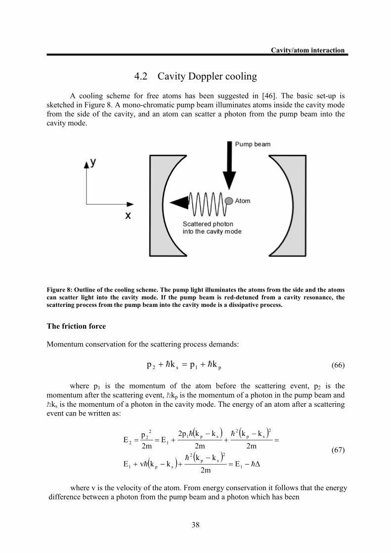
4 Cavity/atom interaction
In this chapter, the subject is the interaction between atoms with a position inside the
cavity mode and the light in the cavity mode. The simplest interaction between atoms in the
cavity mode and the cavity mode is the dipole force on atoms from light in the cavity mode,
and this is discussed in chapter 4.1. In chapter 4.2 is explained how a cavity mode can be used
to cool atoms, which are not spatially confined (cavity Doppler cooling). Chapter 4.3
discusses self-ordering of initial free atoms, and in chapter 4.4 side band cooling of atoms in
the Lamb-Dicke regime is discussed. In chapter 4.5 cavity cooling with two cavity modes is
discussed and in chapter 4.6 the measurement of the normal splitting with a far detuned probe
beam is discussed.
4.1 Optical dipole trap
Using optical dipole forces to capture neutral atoms is a standard method to tightly
confine an atomic sample spatially with a long storage time. An introduction to far red-
detuned optical dipole traps is given in [48]. Chapter 3 described how a strong electrical field
can be build up in a cavity mode. The electrical field in a cavity mode can create a spatial
confining potential for an atom if the frequency of the cavity mode is red-detuned to an
atomic resonance.
The potential energy of a neutral atom in a light field
In the case where the cavity mode is far red-detuned from an atomic resonance, the potential
is given by [48]:
)r(I2
c3)r(U cavity3
0
2
dip
rr
∆γ
ω
π= (56)
where γ is the linewidth of the atomic transition, ∆ is the detuning from the atomic
resonance (∆ < 0 for red-detuning) and )r(I cavity
r is the intensity of the electrical field in the
cavity mode. By adding the two directions of the cavity mode together (see equation 37) and
taking into account the cavity enhancement, )r(I cavity
r can be estimated near the focus as (i):
20
22
w
yx2
2
2
0
inCavity e)kz(Sinw
P2Ab)z,y,x(I
+−
π= (57)
where bin is the fraction of the incoming beam, which is transmitted into the cavity
mode.
i ( ) 0
222 zzand2R(z)yxk <<<<+
Page 37
36
Cavity/atom interaction
The potential energy of a neutral atom in a Gaussian standing wave in the harmonic
approximation
The second order Taylor expansion of equation 56 is:
22
z
22
y
22
xdip zm2
1ym
2
1xm
2
1U)r(U Ω+Ω+Ω+=
r (58)
where ∆γ
ω
π
π=
3
0
2
2
0
in2
c3
w
P2AbU , m is the mass of the atom,
m
U2kz =Ω and
m
U
w
2
0
xy =Ω=Ω . The potential given by equation 58 is the one for the linear harmonic
oscillator and each dimension can be treated separately. The eigenstates of the linear
harmonic oscillator in one dimension can be written as [49]:
Ω
πΩ
=ψ= π
Ω−
−x
mHe
m
!n2
1)x(n n
2
m
4n
nhh
(59)
where n is an integer (n≥0) and Hn is the Hermite polynomial of the order n. The
eigenstates n can be understood as different vibrational levels in the harmonic oscillator and
the energy of each state is given by [49]:
)n2/1(E zn +Ω= h (60)
Correction term of the energy of the vibrational levels
In the harmonic oscillator the energy difference between the vibrational level 1n + and the
vibrational level n does not depend upon n, however, this is only true as long the higher
order terms in the Taylor expansion are not considered. The extra potential terms in the fourth
order Taylor expansion are:
( )
++= 4
444
4
0
z3
kyx
w2
1U)z,y,x('U (61)
The shifting of the energy (∆En) of the eigenstate n can be estimated by treating
)z,y,x('U as a perturbation.
Page 38
37
Cavity/atom interaction
The first order approximation for the energy shift (∆Ez,n) on the z-axis for zn is [49] :
m8
k)1n2n2()1n2n2(zUknzn
3
kUE
22224
0
4
z
4
z
4
n,z
h++=++==∆ (62)
where z
0m2
zΩ
=h
. The energy difference ( )n,1nE +∆ between the states 1n + and
n is:
( )m2
kn1E
22
zn,1n
hh ++Ω=∆ + (63)
Heating of neutral atoms in a dipole trap due to scattering
An atom captured in the dipole trap by the cavity mode will scatter light from the cavity mode
into free space. The random recoils heat the atom and the heating rate is given by [48]:
( )2
0
2
3
0
22
free
22
heat4))r(s1(
)r(s
m2
k,rI
m
k2P
∆++γ
γ=∆= v
vhrh
(64)
where 0
cavity
0I
)r(I)r(s
rr= , ),r(I free ∆
r is the free space scattering rate and I0 is the
saturation intensity of the atom. The trap depth of a bound atom in the dipole trap can be
estimated by:
Bk3
U2T = (65)
Page 39
38
Cavity/atom interaction
4.2 Cavity Doppler cooling
A cooling scheme for free atoms has been suggested in [46]. The basic set-up is
sketched in Figure 8. A mono-chromatic pump beam illuminates atoms inside the cavity mode
from the side of the cavity, and an atom can scatter a photon from the pump beam into the
cavity mode.
Figure 8: Outline of the cooling scheme. The pump light illuminates the atoms from the side and the atoms
can scatter light into the cavity mode. If the pump beam is red-detuned from a cavity resonance, the
scattering process from the pump beam into the cavity mode is a dissipative process.
The friction force
Momentum conservation for the scattering process demands:
p1s2 kpkp hh +=+
(66)
where p1 is the momentum of the atom before the scattering event, p2 is the
momentum after the scattering event, —kp is the momentum of a photon in the pump beam and
—ks is the momentum of a photon in the cavity mode. The energy of an atom after a scattering
event can be written as:
( ) ( )
( ) ( )∆E
2m
kkkkvE
2m
kk
2m
kk2pE
2m
pE
1
2
sp
2
sp1
2
sp
2
sp1
1
2
2
2
hh
h
hh
−=−
+−+
=−
+−
+==
(67)
where v is the velocity of the atom. From energy conservation it follows that the energy
difference between a photon from the pump beam and a photon which has been
Page 40
39
Cavity/atom interaction
scattered into cavity is ∆h . If ∆ is positive the process of scattering photons from the pump
beam into the cavity mode is dissipative.
The momentum transfer of the process of scattering from the pump beam into the
cavity mode is the vector ( )sp kkp −=∆ h , and since both beams affect the direction of the
momentum transfer, it is a called a two photon process.
The pump beam is retro-reflected, and the k-vectors for the two directions are: ± ky.
The k-vectors for the two directions for the cavity mode is: ± kx. Scattering of light from the
pump beam with +ky to the cavity direction with +kx is called the ++ scattering event.
The frequency of the emitted photon by one of the four scattering events can be
calculated from equation 67 by inserting the appropriate k vectors for the scattering event
considered. The detuning of the emitted light into a cavity mode in terms of the detuning of
the pump light to the cavity mode (δ) for one of the four scattering events is [46]:
( ) ( ) δ'vkkm
kδvkkδ yx
2
yx +⋅±−=−+⋅±−=±± mh
m (68)
Figure 9: Detuning of the pump beam (δδδδ) to a cavity mode.
Only one cavity mode is considered, and it is assumed that the intensity in the cavity
mode is too small to affect the distribution of the atoms inside the cavity mode. The atoms are
assumed to be positioned at the focus of the cavity mode.
With the detuning of the emitted photon to the cavity mode known from equation 68,
the scattering rate can be calculated from equation 49. The scattering of photons from a pump
beam into one of the directions of the cavity mode is a series of discrete momentum changes,
where the time interval between two scatterings from the same pump beam into the same
direction of the cavity mode is τcavity.
Page 41
40
Cavity/atom interaction
If instead the series of discrete momentum changes is assumed to be a continues
momentum change over time, it is possible to write this as a continues force on an atom in the
cavity mode:
( ) ( ) ( ) ( )( ) ( ) ( ) ( )yxk,kyxk,k
yxk,kyxk,k
kk∆ωΓkk∆ωΓ
kk∆ωΓkk∆ωΓf
yxyx
yxyx
+−++−++
++++−+=
−−+−
−+++
hh
hh
(69)
where Γ(ω) is the scattering rate from one of the pump beams into one direction of the
cavity mode, and where ω is the frequency of the emitted photon. If ω is equal to the
frequency of the cavity mode, the scattering rate into one direction of the cavity mode is
)(Γη2
)(Γη)(Γ free0
freec ω=ω
=ω . Γfree(ω) is the spontaneous emission rate into free space due
to scattering from one of the pump beams. The factor ½ is due to the fact that only scattering
into one direction of the cavity mode is considered. If the pump beam is detuned relative to
the cavity resonance, the scattering is lowered by the factor
−+
2
c
∆υ
υω11/ , (see equation
54).
As only one mode of the cavity is considered, it is more obvious to write the
frequency ω in terms of the detuning to the cavity mode considered. The scattering rate from
scattering one of pump beams into one direction of the cavity mode is [46]:
( )2free
0/∆δ1
Γη)Γ(δ
υ+=
±±
±± (70)
By inserting the expression for the scattering rate into equation 69, the force along the
vectors (kx-ky) and (kx-ky) can be calculated [46]:
( ) ( )( )( ) ( ) ( )
( )( )2222
yx
2
0freeyx2222
yx
2
0freeyxδ∆υδ∆υ
vkk∆υ4δδηΓkk
δ∆υδ∆υ
vkk∆υ4δδηΓkkf
+−−+−−++ ++
⋅+++
++
⋅−−= hh (71)
If δ' (see equation 68 for the defnition) is negative, the force on an atom along the
vectors (kx±ky) will be opposite of the projection of the velocity of the atom on these vectors.
In other words f for negative δ’ is a friction force.
In Figur 10 the friction force along the k-vector (+kx-ky) is plotted as a function of the
Doppler shift when δ’ = -∆ν is shown. k is the length of the k-vectors (+kx±ky). The capture
velocity is defined as the velocity where the friction force has the largest amplitude.
Page 42
41
Cavity/atom interaction
Capture velocity
From equation 71, the capture velocity along the k-vector (kx±ky) can be calculated:
k
δ'
3
1
∆υ
δ'
3
1
∆υ
δ'
∆υ
δ'1
3
2
k
∆υv
242
capture ≈−
+
+
+= (72)
where the approximation is valid when δ’/∆ν >> 1.
-10 -5 0 5 10
-0.5
0
0.5
Hkx-kyL vêDn
fIkx-k yM
hk2
h 0G
free
Figure 10: The friction force on an atom in the cavity mode as a function of projection of the velocity of
atom on the k-vector (kx-ky) . The detuning (δδδδ’) is ∆∆∆∆νννν.
Heating rate due to random recoils
The friction force given in equation 71 states that it should be possible to cool an atomic
sample to the absolute zero. This unphysical result is due to the assumption that the force on
atoms is acting continuously on the atoms and not in a series of discrete momentum kicks.
The heating rate due to the discrete nature of momentum changes can be estimated by
calculating the heating rate for an atom at T = 0 (e.g. the Doppler shift is set to zero).
Page 43
42
Cavity/atom interaction
The energy change for one scattering event for an atom with v = 0 according to
equation 67 is: ( )
2m
kk2
sp
2 −h. If the frequency difference between the pump beams and the
cavity mode is small, the energy change can be approximated to: m
k2
p
2h
. The scattering rate
for the four possibilities are the same for v = 0 and is given by equation 70.
The heating rate from scattering from the pump beams into the two directions of the
cavity mode is:
( )2free
2
p
2
0
2
p
2
cavityheating,/∆δ'1
Γ
m
k4η)Γ(δ'
m
k4γ
υ+==
hh (73)
The cooling rate due to scattering from the pump beams into free space is the same as
the heating rate for standard Doppler cooling. The absorption of a photon from a pump beam
and the spontaneous emission can be treated as two different momentum changes and the
momentum change for each process is: 2m
k2
p
2h
.
The heating due to scattering from both pump beams into free space is:
free
2
p
2
freeheating, Γ2m
k4γh
=
(74)
The total heating rate at T = 0 due to the pump laser beams is:
( )
+
υ+= 1
/∆δ'1
2η
m
k2Γγ
2
0
2
p
2
freeheating
h
(75)
The Doppler temperature
The kinetic energy of an atom in steady state can be estimated by setting the cooling rate for
an atom with the velocity v ( )vf ⋅ equal to the heating rate at T = 0.
( )( ) ( )
( )
( )( )
( )( )( )
+
≈υ+
++≈
++
+
+=
⇔
+
υ+==
++=⋅
−−++
−−++
−−++
∆υ
δ'
δ'
∆υ
2
∆υ
/∆δ'1
1
∆υδ'2
δ∆υδ∆υ
δ∆υδ∆υ
2k∆υδ'4ηΓ
1/∆∆δ'1
2ηkΓ
mv2
1
1/∆δ'1
2η
m
k2Γγ
δ∆υδ∆υ
vk∆υδ'4ηΓvf
22
2222
2222
2
p
2
0free
2
02
p
2
free
2
2
0
2
p
2
freeheating2222
222
0free
h
h
h
h
hh
(76)
Page 44
43
Cavity/atom interaction
In the first approximation in equation 76 it is assumed that γheating, cavity >> γheating, free. In
the second approximation in equation 76 it is assumed that vk>>'δ . With these
approximations the minimum kinetic energy has its minimum when υδ ∆=' and the kinetic
energy for the atom in this case is υ∆h .
The Doppler temperature is defined as:
B
cavityDoppler,k
∆υT
h= (77)
The Doppler temperature gives an estimation of which temperatures that can be
reached with cavity cooling.
Advantages of cavity cooling
In standard Doppler cooling on an atomic transition the Doppler temperature is [50]:
B
transitionatomicDoppler,2k
γT
h= (78)
where γ is the linewidth of the atomic transition of the cooling transition. The
linewidths of the cooling transitions used in standard Doppler cooling are typically several
MHz [50] and the corresponding Doppler temperatures are around 100 µK. The cavity
linewidth is decided by the finesse and the length of the cavity, and it is possible for large
open cavities to have a linewidth of a few kHz. From the comparison of the Doppler
temperature for standard Doppler cooling and the one possible in cavity cooling one can
expect, that an atom can be cooled to a much lower temperature with cavity cooling than with
the standard Doppler cooling and this is one of the major advantages of cavity cooling.
Another advantage of cavity cooling compared to standard Doppler cooling is that in
cavity cooling the detuning of the pump beams can be chosen to be far away from any atomic
transition. This means that the scattering of light from the pump beams into the cavity mode
does not change the internal state of the atom significantly. This avoids the problem of the
atom decaying to a dark state for the cooling light as in a MOT. The only demand for an atom
or a molecule to be cooled by cavity cooling is that Γfree(ω) > 0. If the atom or molecule can
be polarized, there will always be frequencies ω where the free space scattering rate is not
zero.
If the pump beams are far detuned from any atomic transition, cavity cooling does not
have the same density limitation as standard Doppler cooling has. The scattered photons from
the pump beams into free space are also far detuned and the internal pressure these photons
create on an atomic sample is much smaller than if these photons had been resonant.
Page 45
44
Cavity/atom interaction
Relevant experimental parameters for the cavity
Parameter Value
Cavity Doppler temperature 500 nK
Capture velocity (vc) with δ’ = ∆ν. 7.8 mm/s
Capture temperature b
2
c
k2
mv
320 nK
Recoil temperature at 780 370 nK
Cooling rate 3 µK/ms
Table 2: The cooling rate for the cavity presented in this thesis is calculated with a detuning of one
linewidth relative to a cavity mode, the velocity of the atom is the capture velocity, an atomic detuning of 5
GHz and a pump intensity of 107 mW/cm
2.
4.3 Self-organization of atoms in a cavity
In the derivation of the cooling force in the previous sub-chapter, the electrical field
that can build up inside the cavity due to scattering from the pump beams into the cavity
mode was neglected, and this omits a very important aspect of the cavity. The field inside the
cavity is a standing wave and if the cavity mode is red-detuned to an atomic transition, the
potential minimums are at the anti-nodes of the standing wave. For a sufficiently strong
electrical field in the cavity mode, this will force a periodic ordering of the atoms along the
propagation direction of the cavity mode.
The periodicity of the atomic distribution depends on the interaction between the
atoms in the cavity mode, the pump beam and the cavity mode. In [51] it is shown that for a
certain choice of the parameters of the cavity mode and the pump beam, a threshold of the
intensity of the pump beam exists above which the periodicity of the steady state atomic
distribution inside the cavity mode is λ where λ is the wavelength of the cavity mode. In this
thesis, self-organization is understood as the process by which the atomic distribution goes
from an initially even one to a one with a periodicity of λ.
When the atoms are ordered λ apart, the photons emitted by the atoms into the cavity
mode are all constructively interfering and this greatly enhances scattering [52]. In [53] a
factor 2000 difference in the emission intensity from the atoms into the cavity mode above a
certain threshold intensity of the pump beam was observed.
The equations describing the interaction between a cavity mode and an atom
The theory of self-organization is discussed in [51,54,55,56,57,58], and in these papers the
Heisenberg-Langevin approach is used to describe the interaction between the atoms, a cavity
mode and the vacuum modes. A text book introduction to the Heisenberg-Langevin approach
can be found in [43]. The electrical field in the cavity mode is assumed to be classical, while
the atom is treated as a two level quantum system (semi-classical model). In the limit of a
large detuning of the pump light from an atomic transition compared to the linewidth of the
atomic transition, the excited state can be adiabatically eliminated.
Page 46
45
Cavity/atom interaction
From these assumptions the following equations can be written as [51]:
∑∑∑ +−
Γ+−
−=
j
jpeff
j
jp
j
jp zkCoszkCoszkCosUidt
dαξηακαδ
α)()()( 2
0
2
0 (79)
( ) ( ) ( ) jjpeffêffjp
22
0
j)zk(Cos
dz
di)zk(Cos
dz
d
2
1U
dt
dpξ+αη−αη−
−α−= ∗∗hh (80)
where α is the number of photons in the cavity mode. pj is the momentum of the atom
with the number j (j = 1,2,…,N), zj is the position of the atom with the number j on the
propagation direction of the cavity mode,22
A
A
2
0
gU
γ+∆
∆= is the frequency shift of the cavity
mode due to one atom in the cavity mode, 22
A
2
0
g
γ+∆
γ=Γ is the scattering rate from one atom
in the cavity mode into free space, A
effi
g
∆−γη
=η is the effective pumping rate, η is the
pumping rate, ∆A is the atomic detuning of the pump beam, g is the coupling strength between
an atom and the cavity mode
ε
ω=
eff
c
V2dg
h, d is the atomic dipole moment, κ is the decay
rate of the electrical field of the cavity mode, and ξ are the noise terms due to scattering into
free space. A discussion of the derivation of the equations for dt
dα and
dt
dp j can be found in
[54,56].
The potential energy of the atoms in the cavity in the mean-field approximation
The self-organization can be understood by the conservative terms in equation 80. In [57] the
assumption is made that the cavity field instantly adjusts to the position of the atoms (mean-
field approximation). From this assumption, the potential seen by an atom in the cavity mode
is:
)zkcos(U)zk(cosU)z(V p1p
2
2 += (81)
where ∑=j
jp
2
00
2
2 )zk(CosUINU h , ∑∑
−δ=
j
jp
j
jp
2
001 )zk(Cos)zk(CosNUIN2U h
and ( ) ( )20
2
0
2
eff
0NUN
I−δ+Γ+κ
η= is the maximum number of scattered photons into the
cavity mode for an atom. If the distribution is not completely even, then 0U1 ≠ . If both U2
and U1 < 0 then )kz(cosU 2
2 and )kzcos(U1 have the same sign for kz = 2nπ and opposite
Page 47
46
Cavity/atom interaction
sign for kz = (2n+1)π. If the detuning is chosen such that 0)zk(CosNUj
jp
2
0 <−δ ∑ the
sign of U1 is the opposite of the sign of ∑j
jp )zk(Cos . For U1 to be negative ∑j
jp )zk(Cos
must be greater than zero, which means that the atoms must be closer to the points with
k
n2πcompared to the points with
k
)1n(2 +π in order to obtain a sum that is greater than zero.
If there are initially more atoms close to even sites (2n) than at the uneven sites
(2n+1), this imbalance creates a stronger confinement at even sites and a weaker confinement
at the uneven sites. This imbalance in confinement leads to more atoms at the even sites than
at the uneven sites and this in turn creates a greater difference in the confinement between the
even and uneven sites. The process that an uneven distribution creates an uneven confinement
which then amplifies the difference in the distribution between the even and uneven sites is
the physical mechanics for self-organization process.
Threshold power of the pump beam for the self-organization
Thermal fluctuations counteract the self-organization process, and only at a certain intensity
of the pump beam, the self-organization process can occur. The depth of the potential of the
standing wave of the cavity mode is given by U. In order to confine the atoms at the anti-
nodes the following must be true U > kbT where T is the temperature of the atomic sample in
the dipole trap. From this condition, the power in the cavity mode can be estimated to be
(Pcavity):
γ
∆
3c
TkωwPTkU a
2
b
3
c
2
0cavityb >⇔> (82)
In steady state the energy scattered from the pump beam into the cavity mode must be
equal to the decay of the cavity field.
The cavity field can decay through two methods: loss process at the mirrors
(transmission or scattering loss) or by light scattered from the cavity mode into free space by
atoms in the cavity mode.
cavityccavitypumpcc NhPNh Γω+χ=Γηω (83)
where Γpump is the scattering rate into the cavity mode due to the pump beam, χ = χ0 +
χ1 + χ2 is the total losses at the mirrors, N is the number of atoms in the cavity mode and
Γcavity is the scattering rate from the cavity mode into free space. In the limit of large atomic
detuning compared to the natural linewidth and a low saturation, equation 83 can be written
as:
4
3
a
c
sat
22
0
2
c
b
22
0
sat3
2
a
cc
sat
22
0
2
c
cavity
satpump
∆
Nh3
Iw
NhTkkw
I∆
Nh
Iw
NhP
IIγη
∆π
γω+χ
>γηω
∆π
γω+χ
= (84)
where Isat is the saturation intensity.
Page 48
47
Cavity/atom interaction
The power needed for self-organization according to equation 84 has to be greater than
10 µW/cm2 with an atomic detuning of 30 nm, a temperature of 1 µK of the atomic sample in
the cavity mode, an atom number of 105 and the cavity parameters can be found in Table 11.
When the atoms self-organize into an atomic distribution with a periodicity of λ, one can
expect the scattering rate to increase and thus the threshold for self-organization should
therefore be lower than the one predicted from equation 84.
The superradiant and the strongly coupled regime for a self-organized sample
In [55] the dependence of Icavity on the cavity decay rate, the atomic detuning and the atom
number is discussed. The power of the pump beam is assumed to be above the threshold for
the self-organization, and the atomic sample is assumed to have self-organized into a
distribution with the periodicity of λ. With the same assumption as the ones for equation 84,
Icavity can be written as:
( )( )δκ−γκ+κ+∆+δ 82Ns4sN4
N~I
22
a
222
2
cavity (85)
where 2
a
2gs
∆= . From Figure 11 two different regimes can be identified. When N <<
N0, the coupling between the atomic distribution and the cavity mode is weak and the
dependence of the intensity in the cavity mode on the atom number is N2 (superradiance).
When the atom number is above N0 the coupling between the atomic distribution and cavity
mode is strong. The intensity of the cavity mode becomes independent of the atom number N
in the strong coupling regime because the reason is that the atoms are sitting in the dark. The
cavity field and the pump field are of the same order of magnitude in the strongly coupled
regime and they destructively interfere [55,58].
The dependence of the N0 is given by:
( )γκ−∆δκ+δ
=a
22
04s
4N (86)
Page 49
48
Cavity/atom interaction
0 0.5 1 1.5 2 2.5 3.
0
1
2
3
Atom number H105 L
Cav
ity
inte
nsit
yHA
rb.
Uni
t.L
Figure 11: Photon number in the cavity mode in steady state with the atoms illuminated by a pump beam
from the side. The atomic sample is assumed to have self-organized into a distribution with a periodicity
of λλλλ (see equation 85). The values for the cavity can be found in Table 11, and the atomic detuning (∆∆∆∆a) is
set to 30 nm. The peak intensity in the cavity mode is at 0 = 6 104.
The transmitted power through out-coupling mirror in the limit of large
When N >> N0 the pump beam and the cavity mode have the same intensity at the position of
the atoms as they cancel each other in the centre of the cavity mode. From this condition the
power in the cavity mode can be calculated as the intensity in the cavity mode in the centre is
the same as the one of the pump beam. By multiplying the transmission coefficient (χ2) of the
out-coupling mirror (see Figure 7) with the power in the power in the cavity mode, the power
of the transmitted beam through that mirror can be estimated. Ip is the intensity of the pump
beam and Pt is the power of the beam transmitted through the out coupling mirror:
2
0p2t wI2
Pπ
χ= (87)
An intensity of the pump beam of 105 W/cm
2, a waist of 30 µm and δ2 = 1 ppm gives
an estimate for Pt of 1 nW.
Page 50
49
Cavity/atom interaction
Cancelling the potential variation along the propagation direction of the cavity mode
In chapter 5.10 it is explained how to keep a fixed detuning of the pump beam to a cavity
mode. To achieve this technically it is necessary to have a laser beam resonantly locked to a
cavity mode. The in-coupled beam will create a standing wave inside the cavity. For the self-
organization process to occur, the depth of the potential of the standing wave due to the
directly in-coupled light must be comparable to or smaller than the kinetic energy of the
atoms.
If the potential wells are much deeper than the kinetic energy, the atoms are locked
into an atomic distribution with a periodicity of λ/2 with a very low probability to tunnel from
one lattice site to the next.
From the potential depth (U0) given in equation 56, the in-coupled power (P) must be
10 pW for an atomic detuning of 30 nm and in-coupled ratio of 1 (bin) in order to be equal to
the recoil temperature of Rb87.
A method to suppress the potential along the cavity axis is to couple a second laser
beam into the cavity through a mirror with a frequency difference of one free spectral range
(∆q=1, see equation 43) compared to the cavity mode, which the first laser beam is locked to.
The wavelength of the first laser beam is given by: L2q 1 =λ and the wavelength of
the second laser beam is given by: ( ) L21q 2 =λ+ . As the width of the BEC is of the order
100 µm along the propagation direction of the cavity mode and the Rayleigh length (z0) of the
cavity mode is 3 mm, the intensity can be assumed to be constant over the atomic sample near
the waist of the cavity mode. Thus, the intensity of the electrical field of both cavity modes
near the waist (z ≈ L/2) is:
( ) ( ) ( ) ( ) t)∆ω(CoszkSinzkSin2zkSinEzkSinE
z)eSin(kEz)Sin(kEz)eSin(kEz)eSin(kEt)I(z,
212
22
21
22
1
2 t∆ω i
2211
2tiω
22
tiω
11211
++
=+=+= (88)
∆ω is one free spectral range (3 GHz) and it is much faster than all other timescales
relevant in the self-organization process. Therefore, the intensity can be averaged over one
oscillation period (2π/∆ω), and the last term in equation 88 has a time average of zero.
( ) ( )
π
π−
π+
π=
π−
π+
π≈
π
π+
π≈
π+
π+
π=+=
xL
nCosEx
L
nx
L
nCosEx
L
nSinE
xL
n1x
L
nCosEx
L
nSinEx
LSinx
L
nCosEx
L
nSinE
xL
xL
nSinEx
L
nSinEzkSinEzkSinEI(z)
22
2
2
22
2
22
1
2
22
2
22
1
222
2
22
1
22
2
22
12
22
21
22
1
(89)
For E2 = E1 the potential variation along the propagation direction near the waist is
suppressed by a factor µm 100for x 10 4xL
πa 6-
2
=≈
= compared to the situation without a
Page 51
50
Cavity/atom interaction
second laser beam coupled in. Depending on the achievable stability of the two laser
intensities it is possible to stabilize with a much higher power than the 10 pW, and there is
still no lattice along the propagation direction of the cavity mode at the position of the BEC.
In the directions perpendicular to the propagation direction of the cavity mode, the
confinement near the waist is the same as for only one laser beam coupled in.
0 0.5 1 1.5 2 2.5 3 3.5 4 4.5 5
0
0.5
1
1.5
2
z HcmL
Inte
nsit
ypr
ofil
eHa
.u.L
Figure 12: Intensity profile inside the cavity along the propagation direction of the cavity mode. The
length of the cavity is set to 5 cm. The intensities of both laser beams are equal.
Relevant parameters for self-organization
Parameter Value
Threshold intensity for self-organization 10
µW/cm2
Number of atoms for strong coupling at
30 nm detuning from an atomic resonance
(N0)
6 104
Expected transmitted power through
outcoupling mirror with pump intensity of
105 mW/cm2 (Pt)
1 nW
Table 3: The atomic detuning is 30 nm.
Page 52
51
Cavity/atom interaction
4.4 Cavity sideband cooling
Atoms tightly bond in a harmonic trap can be cooled by illuminating them with a
pump beam. The pump beam can induce transitions from one vibrational state of the atom to
another state. The symmetry between the probability for a transition from the initial state to a
vibrational state with more energy (heating transition), and the probability for the transition
from the initial state to a vibrational state with less energy (cooling transition) can be broken
by the cavity. This asymmetry can be used to cool an atom by making the cooling transition
more likely than the heating transitions.
Emission spectrum of a bound atom
Laser cooling of bound atoms is described in [59,60]. The electrical field of the radiation from
an atom in the cavity mode into one of the directions of the cavity mode is:
( ) ( )ωtzkSinEtz,E p0 −=rr
where 0Er
is the maximum electrical field along the propagation
direction of the cavity mode and ω is the frequency of the emitted light for an atom at rest
with respect to the cavity.
Figure 13: Sideband cooling of bound atoms in a harmonic potential. The cavity breaks the symmetry
between scattering events, which heat an atom (red arrow), and the scattering events that cool an atom
(blue arrow).
The oscillation of a bound atom in a harmonic trap is: ( )zza φtΩSinzz(t) += where
Ωz is the oscillation frequency for the harmonic trap, za is the amplitude of the oscillation and
ϕz is the phase, which can be set to zero since only one atom is being considered. Then the
electrical field emitted by the atom is: ( ) ( )( )ωttΩSinzkSinEtE zap0 −=rr
. The electrical field
( )tEr
can be expanded as: ( ) ( ) ( )( )tjΩωSinzkJtE z
j
ap
2
j += ∑∞
−∞=
r, where j is an integer and
Jj(kpza) is the Bessel function of the first kind [59]. If kpza << 1 (the Lamb Dicke Limit) is
valid, the amplitude of the sidebands ω±Ω is much larger than the amplitude of the sidebands,
where 2j ≥ .
Page 53
52
Cavity/atom interaction
Figure 14: The amplitudes of the sidebands for kpza = 1.
The cooling rate for a single sideband for an atom in the classical limit
The cooling (heating) rate for scattering from the pump beam into the sideband ω+jΩ is [59]:
( ) ( )ap
2
jjwz zkJδIjΩdt
dEh−= (90)
where z
2
p
j jΩ-m
kδδ
h−= , δ is the frequency difference between the pump beam and
the cavity mode, ( )jw δI is the scattering rate into the cavity mode at the detuning δj and
( ) ( )2j
free0ap
2
j/∆δ1
ΓηzkJ
υ+ is the scattering rate from the pump beam into one direction of the
cavity mode with the frequency (ω+jΩ). As in cavity Doppler cooling the random recoils heat
the atom and each recoil heats an atom at rest with m
k2
p
2h
.
The total cooling (heating) rate is:
( ) ( )2j
free0ap
2
jx
2
p
2
/∆δ1
ΓηzkJjΩ
m
k
dt
dE
υ+
−= h
h (91)
equation 91 is only valid when the energy of the atom is high compared to the energy
of the ground state
Ω z2
1h .
The cooling rate for a single sideband for an atom quantum mechanically
To calculate the cooling (heating) rate at low temperatures the scattering rate from one
vibrational state to another has to be calculated by quantum mechanics.
Page 54
53
Cavity/atom interaction
The eigenstate with the energy En of the atom in the harmonic trap, and N photons in
the cavity mode with the frequency (ω+jΩ) is written as N,n . If the atom is at the focus,
and the only field along the propagation direction is considered (y = x = 0), the electrical field
for one direction of the cavity mode can be approximated to ( ) h.c.aeiεt)E(z, tωkzi
max += + (see
equation 50).
The scattering rate for the transition from the state 1,'n to the state 0,n is given by
Fermi Golden Rule:
( ) ( ) ( )
)j(τ
1n'en
1aiε0nen'jωρ2π
n,0t)E(z,,1n'ωρ2π
τ
1
cavity
2ikz
2
max
2 tωkzi-2
j
Ω+ω=
Ω+== +
Ω+ω hh (92)
where )j(τ
1
cavity Ω+ω is the scattering rate from the pump beam into one direction of
the cavity for a free atom. From equation 92 it follows that in equation 91 the term ( )ap
2
j zkJ
must be substituted with 2
ikz n'en in order to obtain the cooling (heating) rate for the
transition from the vibrational state n to the vibrational state 'n .
The cooling rate of a thermal sample
An estimate for the cooling (heating) rate at a given temperature can be found by averaging
equation 91 over a thermal distribution:
( )( )∑∞
=
υ
−+
−=
0'n,n2
2
z
free0
2ikz
z
2
p
2
n
∆
Ωn'-n-Rδ1
Γηn'en)Ωn'-(n
m
kp
dt
dEh
h (93)
where pn is the probability for the atom to be in the vibrational state n and
m
kR
2
ph= . It was required to evaluate equation 93 in the limit of low temperatures. At low
temperatures it is possible to assume that all the relevant eigenstates are strongly bound in the
trap ( )1nznk 2
p << and with this assumption 2
zikn'en p can be approximated to
2
n'ikz1n + . The matrix elements can be evaluated as: 'nn,1bznn'zn −δ= and
'n,n'nn δ= , where z
bm2
zΩ
=h
is the width of the ground state [59].
The detuning δ of the pump beam is chosen such that the scattered photon from the pump
beam into the sideband ω+Ω is resonant with the cavity ( )Ω+=δ R , and it is assumed
Page 55
54
Cavity/atom interaction
that: zΩ >> R and zΩ >> ∆ν. From these approximations, the cooling rate at low temperatures
can be estimated as:
−
υ
≈
−
υ+
υ+≈ ∑
∞
=
z2
z
22
p
2
free0
0n
2
p
2
bz2
z
22
p
2
2
z
22
p
2
bznfree0
n2
1
8Ω
9∆
m
kΓη
nkzΩΩ
∆
m
k
4Ω
∆)1n(kzΩpΓη
dt
dE
h
hh
h
(94)
where ∑∞
=
=0n
nz npn . The cooling rate in equation 94 is valid for scattering from one
direction of the pump beam into one direction of the cavity mode. The total cooling rate for
scattering from both directions of the pump beams and into both directions of the cavity mode
is 4 larger than the rate given in equation 94.
The heating rate due to scattering from the pump beams into free space is given by
equation 74 and the total cooling rate is then:
−
υ+≈ z2
z
2
0
2
p
2
free0 n2
1
8Ω
9∆
2η
1
m
kΓη
dt
dE h (95)
The steady temperature
The steady state is found by setting 0dt
dE= :
2
z
2
0statesreadyz
8
91n
Ω
υ∆+
η= (96)
The temperature of the steady state is given by:
Ωυ∆
+ηΩ
=Ω
=z
2
0
z
BB
statesreadyzz
8
9
k
h
k
nhT (97)
umber of vibrational states that can be simultaneously cooled
In equation 63 the energy difference between the vibrational states 1n + and n due to the
fourth order terms in the potential was calculate. From this calculation, one can see that if the
pump beam is resonant with the transition from 1 to 0 , the pump beam has a detuning to
the transitions from 1n + to n vibrational states.
Page 56
55
Cavity/atom interaction
The number ncapture where the detuning is less than the linewidth of the cavity can be
estimated from equation 98:¨
2capture
22
capturek
m2n
m2
kn
hh
h ν∆=⇔ν∆= (98)
From equation 98 one can see that ncapture is the number of random recoils the atom can
undergo before it moves out of resonance. In cavity Doppler cooling the number of random
recoils the atom can undergo, before the Doppler shift is too large for the atom to be resonant
with the transition from the pump beam to the cavity mode, is the same as the one in equation
98.
Parameters relevant for cavity sideband cooling with the cavity
In Table 4 the heating rates, the cooling rate and trap parameters for the dipole trap with the
power of the incoming beam at 1 µW (P) are calculated. The heating rate due to lattice is
calculated at the wavelength 825 nm. The saturation of the pump beam (sp) is set to 1000 at
the position of the atomic cloud, and the detuning to D2 line is 0.2 nm red-detuned (10 GHz).
Parameter Value
Ωx , Ωy 45 kHz
Ωx 8.3 MHz
ncapture 2.7
Trap depth 4.7 mK
Pheat 0,15 nK/ms
Psideband, cooling 500 zn
ms
nK
Psideband, heating (z-axis) 30 nK/ms
Psideband, heating (x-axis) 2 µK/ms
statesreadyzn 0.06
statesreadyxn 4.3
Energy of statesreadyzn znµK 25 kb
Energy of statesreadyxn znµK 9,5 kb
Table 4 Parameters for sideband cooling of a single atom. Power of the incoming beam to the in-coupling
mirror is 1 µµµµW.
where m
kΓ2ηP
2
p
2
free0coolingsideband
h= and
υ+=
2
z
2
0
2
p
2
free0heatingsideband4Ω
9∆
η
1
m
kΓ4ηP
h.
The values for the x-axis come from substituting z with x in the relevant equations.
Page 57
56
Cavity/atom interaction
4.5 Cavity cooling with a blue detuned cavity mode
In the previous chapters a laser beam which is red-detuned to a cavity resonance was
considered. Another possibility for cooling is to have two cavity mode with a specific
frequency difference. A dissipative process is created if light is scattered from the cavity
mode with the least frequency of the two modes to the other cavity mode.
Figure 15: Cavity cooling with two cavity modes. The frequency difference between the two modes is δδδδ.
Light is coupled into the TEM00 mode, and when light is scattered from the TEM00 into the TEM22 mode,
energy is transferred from the kinetic energy of the atom to a light field.
Cavity length for frequency degeneracy of a TEM00 and a TEM22 mode
The higher-order Gaussian mode with the highest field per photon in the centre of cavity is
the TEM22 mode. The mode volume of the TEM22 is four times higher than the TEM00 mode,
and due to this the scattering ratio into the TEM22 mode compared to the TEM00 mode is four
times lower. The resonance frequency of a higher-order Gaussian mode is given by [39]:
( ) ( )
++= −21
1
nm,q, ggCosnmπ
1q
2L
cf (99)
According to equation 99, the condition of the g-numbers for a TEM00 mode and a
TEM22 mode to have a resonance frequency at the same length is: ( )4
πggCos 21
1 =− . From
this condition, the length of the cavity can be calculated ( )( )R21L ±= .
Page 58
57
Cavity/atom interaction
Drift of the frequency difference between the two modes due a length change of the
cavity
The frequency change between TEM00 and TEM22 modes due to a small change in the length
of the cavity (∆L) to the first order in ∆L at ( )R21L += is:
L2
c
R
L2f∆
=∆ (100)
Frequency oscillation of the cavity
Because of the fact that the amplitude of the oscillation of the cavity length can be estimated
by locking a laser to a reference cavity (transfer cavity), which one can assume to be
absolutely stable compared to the cavity (experimental cavity), one wish to measure the
oscillation amplitude of (for the set-up see chapter 5.10). The length of the experimental
cavity can be varied by adding a voltage ramp to a piezo, which one mirror of the
experimental cavity is mounted upon. A voltage scan of 33 V changes the frequency of a
cavity mode with one FSR (3 GHz). On the scan of piezo it can be observed that the random
swinging of the cavity mode of the experimental cavity corresponds to 0.2 V applied to piezo,
and from this it follows that the cavity mode at 825 nm has an absolute variation of 20 MHz.
The corresponding length change of the experimental cavity is 3 nm if it is assumed that the
entire swinging of the cavity mode is due to the length change of the experimental cavity. By
inserting 3 nm for ∆L in equation 100 the frequency variation between the TEM00 and the
TEM22 due to the oscillation of the cavity length is 500 Hz. This frequency variation is
significantly smaller than the linewidth of the experimental cavity.
An advantage of using a blue detuned cavity mode for the atoms to scatter into instead
of having a red detuned laser beam is that the in-coupled light can be directly locked to the
experimental cavity with the current lock. The current lock has a much greater frequency span
than the AOM lock where it can follow the oscillation of the cavity mode and it has a much
simpler technical realization. Another experimental advantage of using a blue-detuned cavity
mode is that atoms perfectly overlap with the cooling mode when they are trapped in the
TEM00 mode.
The disadvantage is the extra heating due to having a resonant cavity mode, and the
lower mode volume of a TEM22 compared to a TEM00 mode.
4.6 Normal mode splitting of a ring cavity mode
In the previous chapter a blue detuned higher-order Gaussian mode was suggested to
be used for cooling. One of the disadvantages of using a higher Gaussian order mode
compared to a TEM00 mode for cooling is the higher mode volume. A method to avoid this
problem is to use the normal mode splitting of a cavity mode in the strongly coupled regime
[61].
Page 59
58
Cavity/atom interaction
In the strongly coupled regime between an atomic sample and a cavity mode the
resonance of the cavity mode splits into two resonances. By scattering light from the normal
mode with the lower frequency of the two normal modes into the other normal mode, a
dissipative process can be created. The advantage compared to the method suggested in the
previous chapter is that both normal modes are TEM00 modes. The disadvantage is that the
frequency difference between the two normal modes depend on the atom number, and thus
the resonance condition therefore has to be adjusted when the atom number changes.
The normal mode splitting has been investigated with near resonant probe beams
[62,63]. One of the major advantages of cavity cooling is the possibility to use far off-
resonant light, and the normal mode splitting has been measured with a far off-resonant probe
in a ring cavity [86]. The theoretical background and the results of the measurement of the
normal mode splitting of a mode in a ring cavity with a far off-resonant probe are reported in
this chapter.
The dynamics of atoms in a ring cavity
In [64] the dynamics of N two-level atoms in a weakly pumped ring cavity is
investigated. The two propagation directions in the ring cavity are denoted by + and -, and the
electrical fields for the two directions are given by:
( )( ) ( ) ±=
±± η+α+Γ−α−δ+Γ−κ−=α ∑N
1n
ikz
0000neiUNUiN
m
m& (101)
where ±α is the amplitude of the electrical field of the cavity mode propagating in
the (±)-direction and η± is the pumping strength in the (±)-direction. The other quantities are
the same as the ones in equation 79. For an even distribution along the propagation direction
of the cavity modes: 0eN
1n
ikzn =∑=
m which means that no photons are scattered by the atoms
from one direction into the other. Only forward scattering by the two directions is possible.
For an inhomogeneous atomic distribution the term ∑=
N
1n
ikznem can be different from
zero, and in that case, photons can be scattered from one direction into the other. The number
of photons scattered from one direction into the other direction depend on the number of
atoms and their localization along the propagation direction of the cavity modes. The
localization along the propagation direction of a cavity mode is defined as:
∑=
± ≡N
1n
ikz
ax,ne
N
1ξ
m (102)
When the number of photons scattered from one direction to the other for a perfectly
localized atomic distribution ( )1ξ ax, =± is comparable to the number of forward scattered
photons, the interaction between the atoms and the cavity mode is said to be in the strongly
coupled regime. It is defined as: κ≥0NU .
Page 60
59
Cavity/atom interaction
The steady state solutions of the electrical fields in the two directions of equation 101
are:
( )( ) ( )( )( ) ( )200ax,ax,
22
00
ax,0000
iUξξNNUiN
NξiUNUiN
+Γ−−δ+Γ−κ−
+Γη+−δ+Γ−κ−η=α
±
±±
m
mm (103)
To simplify equation 103, it is assumed that the scattering rate of an atom into free
space can be set to zero (Γ0 = 0). The effective detuning is defined as: δef = δ - NU0. The
atomic distribution is assumed to be periodic with half the wavelength (λ/2) of the cavity
modes and with a phase difference χ to the optical lattice formed by the two counter
propagating cavity modes. In that case χ−χ−
==± ==≡ ∑∑ i
ax
iN
1n
ikzN
1n
ikz
ax, eξeeN
1e
N
1ξ nn mm
where
1ξ0 ax ≤≤ .
ε is defined as the fraction in the intensity pumped into the (+)-direction subtracted the
fraction pumped into the (-)-direction: ( ) ( )222
2
1−+± η+η
ε±=η . The effective coupling
between the optical lattice and the cavity mode is defined as: 0axef UξNg = .
From the mentioned simplifications the electrical field of the two cavity modes are
proportional to [86]:
( )( )( ) ( )( )κ−+δκ−−δ
ε+κ−δε±α
χ±
±efefefef
i
efef
gigi
1eigi1~
m (104)
In the following paragraph ε is set to 1 and the intensity in the (+)-direction is
considered ( )2
+α .
ormal mode splitting
When the coupling between the atoms and the optical lattice is weak
−κ≤ 25g ef , there
is only a single maximum at δef = 0 for ( )( )2
efδα+ . For ( )25 −>κefg the resonance
splits into two and there is a local minimum at δef = 0. When gef >> κ the frequency
difference between the two normal modes (∆ω) is:
0axef UξN2g2 ==ω∆ (105)
The normal mode splitting can be understood in a simple picture. In the strongly
coupled regime an optical lattice is formed due to scattering between the two directions. The
anti-nodes of the optical lattice can either be at the maximums of the atomic distribution or at
the minimums. In the case where the anti-nodes are at the maximums of the atomic
distribution, the interaction is maximized. Similarly if the anti-nodes are the minimums of the
atomic distribution, the interaction is minimized.
Page 61
60
Cavity/atom interaction
Figure 16: The relative frequency of the cavity mode is shown for different atomic distributions along the
propagation direction of the cavity mode. ωωωωc is the frequency of the cavity mode in case of no atoms in the
cavity mode. ωωωωca is the frequency of the cavity mode for an even distribution of the atoms along the
propagation direction of the cavity mode. ωωωωnm and ωωωωol are the frequencies of the two normal modes in the
strongly coupled regime, and for an atomic distribution with a periodicity of λλλλ/2.
If the atomic distribution is perfectly localized at the nodes of the optical lattice, the
frequency of corresponding normal mode is the same as the one for the cavity mode without
any atoms in the cavity mode. The atoms are sitting completely in the dark.
Equation 101 does not accounted for the fact that the atoms are not perfectly localized
radial on the propagation direction of the cavity modes. The radial localization can be defined
as:
( )
∑=
+−
≡ξN
1n
w
yx2
rad
20
2n
2n
eN
1. The effective detuning and the effective coupling are respectively
by including the radial localization: δef = δ - ξradNU0 and 0axradef UξNg ξ= .
The ring cavity set-up
The experimental set-up used to measure the normal mode splitting is a different experimental
set-up than the one described in the other chapters in this thesis. The experimental set-up is a
ring cavity where a cold atomic sample of a few 106 atoms at 100 µK can be loaded into an
optical lattice from a MOT. An optical lattice is created by two counter-propagating modes of
the ring cavity, which are pumped with the same intensity. Only the (-)-direction is kept
resonant with the ring cavity with a PDH lock.
A probe laser phase locked to the laser, which generated the beams for the optical
lattice, was used to probe the transmission spectrum of the cavity with different number of
atoms in the cavity mode. The power of the (+)-direction of the probe beam and the lattice
laser is measured with a photodiode.
An outline of the experimental set-up can be seen in Figure 17, and in [65,71] a
detailed discussion of the entire experimental set-up can be found.
Page 62
61
Cavity/atom interaction
Figure 17: Outline of the experimental set-up. The ring cavity has stable cavity modes propagating in
opposite direction. One direction is denoted as the (+) direction and the other direction as (-). A far
detuned laser (the lattice laser) is coupled into two modes with opposite directions with equal intensity,
and the two counter propagating modes forms an optical lattice. An atomic sample is held in this optical
lattice. A second laser (the probe laser) is used measure the transmission spectrum of the ring cavity, and
the polarization of the probe laser beam is chosen such that the maximum fraction of the light is coupled
to the (+) direction (96,5%). The probe laser is phase locked to the lattice laser, and the technical details
of the phase lock can be found in [87]. The direction (-) is kept with a PDH lock resonant with a ring
cavity mode. PBS = Polarizing beam cube. HWP = Half Waveplate. BS = Beamsplitter.
Parameter Value
Finesse 1.8 105
Waist 97 µm
Cavity linewidth 17 kHz
ηc 0.6
Lifetime of the atomic sample in the optical lattice 300 µs
Temperature of the atomic sample in the optical lattice 123 µK
Trap depth 350 µK
Axial trap frequency 331.1 kHz
Radial trap frequency 459 Hz
Table 5: Parameters for the ring cavity and the properties of the optical lattice of the lattice laser can be
seen in [65,71]. The lattice of the probe laser is not included in the numbers.
Measurement results of the normal mode splitting
The wavelength of the probe and the lattice beams is: 780.9 nm. The transmission spectrum of
the probe laser as a function of the frequency for various atom numbers was measured (see
Figure 18). In Figure 18 the normal mode splitting can be observed at an atom number
slightly above 106 atoms, and 10
6 atoms is the predicted atom number for strong coupling at
the atomic detuning of 0.7 nm. The two normal modes do not have the same amplitude and
this is due to the fact that the probe beam pumps both directions.
Page 63
62
Cavity/atom interaction
If ε = 1, the two normal modes would have identical amplitudes as the term with e-iχ
drops
out of the equation for +α .
Frequency [kHz]
Tra
nsm
itte
d S
ign
al [a
rb. u
nits]
(1)
(2)
(3)
(11)
(10)
(9)
(8)
(7)
(6)
(5)
(4)
10050-50 0
Figure 18: The transmission spectra of the probe laser as a function of the effective detuning of the probe
laser beam for different atom numbers. The traces are numbered from above from 1 to 11 at the bottom.
The corresponding atoms are (0, 0.28, 0.55, 0.83, 1.10, 1.38, 1.66, 1.93, 2.21, 2.48, 2.76) x 106 where trace 1
is for no atoms in the cavity mode. The grey circles are the measured values, and the black lines are the
fitted functions to measure experimental measured values (see equation 106). At each value the
transmitted field was allowed to reach its steady state value.
Page 64
63
Cavity/atom interaction
In Figure 18, the measured intensity at δef = 0 with the highest atom numbers is below
the level when the probe beam is far off resonant with any of the two normal modes. To
explain this phenomenon, the effect on the atomic distribution by the scattering of photons
from the probe beam in the (+)-direction into the (-)-direction has to be included.
A scattering event by an atom of a photon from a mode into the mode of the ring
cavity with opposite propagation direction creates a momentum transfer on the atom, and this
creates a force on the atom. There are four laser beams exerting a force on the atoms: the
lattice beams in the (+) and (-)-directions, and the same for the probe laser beams. The lattice
laser is kept resonant with the (-)-direction of the ring cavity with a PDH lock, and thus it has
a constant in-coupling. 96.5 percent of the power of the probe beam is coupled into the (+)
direction, and in the strongly coupled regime a significant part of the light from the (+)
direction is scattered into the (-) direction.
In steady state the light forces on the atoms must be balanced, and the only possibility
for the forces to be balanced is for the force from the (+) direction of the lattice laser to
decrease if the force on the atoms due to light being scattered from the (+) direction of the
probe beam into the (-) direction increases. It is assumed that the light power scattered from
the (+) direction of the probe beam into the (-) direction is proportional to the light power in
steady state for the (-) direction of the probe beam, which is 2
−α . With this assumption,
the light power measured on the photodiode shown in Figure 17 consists of the two parts: the
transmission spectrum of the probe laser, and the decrease in the intensity in the (+) direction
of the lattice laser due to scattering of photons from the probe laser into the (-) direction.
The light power on the photodiode can be estimated as [86]:
( )22
RSP −+ α−α= (106)
where S is a scaling factor, R is the fraction between the scattering power from the
probe beam and the steady state intensity in the (-) direction of the probe beam. In Figure 18,
the fitting parameters for the plots are: S, R, gef and χ. The fitting parameters for different
atom numbers are plotted in Figure 19, Figure 20 and Figure 21:
Figure 19: The coupling strength for different atoms numbers in the cavity mode. The black boxes show
the strongly coupled regime.
Page 65
64
Cavity/atom interaction
Figure 20: The scattering of photons from the (+) probe beam into the (-) direction first exerts a
significant force on the atoms in the strongly coupled regime, and thus R = 0 in the weakly coupled
regime.
Figure 21: The relative phase between the optical lattice of the lattice laser beams and the optical lattice of
the probe laser beams (χχχχ). When the coupling between the atoms and the cavity modes is weak, the effect
of χχχχ on the transmission spectrum is small. Hence, no reliable value of χχχχ can be found from the
transmission spectrum, when the coupling is weak. The grey area in the plot shows the value of χχχχ due to
different optical path lengths from the beam cube to the in-coupling mirror of the ring cavity (see Figure
17).
In [61,65,71] the possibility to observe cooling with the normal mode splitting is
discussed. The two major experimental obstacles in the ring cavity set-up in order to observe
cavity cooling were a low value for ηc and the short time the resonance condition for the
dissipative process is fulfilled. With a lifetime of 1.7 s and 106 atoms captured in the optical
lattice the resonance condition is only fulfilled for a few ms. As ηc = 0.6 the cooling rate due
to scattering into the cavity mode and the heating rate due the scattering rate into free space
are of the same magnitude.
The major advantage of the new experimental set-up compared to the ring cavity set-
up in regards to cavity cooling is the high value of ηc of the standing wave cavity described in
chapter 5.8.
Page 66
65
Experimental apparatus and procedures
5 Experimental apparatus and procedures
In this chapter the experimental set-up and the procedures used for creating a BEC are
described. In chapter 6 the individual experimental steps for creating a BEC are characterized.
In chapter 5.1 the stabilization on atomic and cavity resonances is discussed, in chapter
5.2 the source of cold Rb87 atoms is described (the first MOT) and in chapter 5.3 the second
MOT is described, which is used to capture the atoms from the cold atomic beam from the
first MOT. In chapter 5.4 the optical pumping set-up is described and in chapter 5.5 the
magnetic traps are described, in chapter 5.6 the two imaging set-ups are explained. In chapter
5.7 the vacuum set-up is shown, in chapter 5.8 the cavity set-up is explained. Chapter 5.9
describes the radio frequency source for evaporative cooling and in chapter 5.10 a system for
stabilizing a laser off-resonant to cavity resonance is described.
5.1 Laser stabilization on atomic and cavity resonances
All laser beams in this experiment are generated by diode lasers. If the laser diode is
used without additional feedback, it is said to be operating in free running mode, and beam
from a free running laser diode is not suitable for operating a MOT for a number of reasons.
Firstly, the width of the emission spectrum is a few MHz, secondly, the emission spectrum is
often far from the desired atomic transition and lastly the laser diode is often running multi
mode. To overcome these problems, additional feedback is created by reflecting some of the
emitted light back into the laser diode by a grating. The external cavity set-up with the grating
is further discussed in the appendix A.
The emitted frequency of the laser diode in the external cavity set-up can drift due to
reasons such as temperature changes or drifts in the current flowing through the diode. In
order to be able to correct the frequency drifts, one must first be able to detect it. This is done
through saturation spectroscopy for stabilization on an atomic resonance [66,67], and for
stabilization on a cavity resonance the reflected light from cavity is used.
Saturation spectroscopy
With saturation spectroscopy it is possible to identify the hyperfine transitions in the spectrum
of Rubidium atoms at room temperature. The Doppler broadening at room temperature of
Rubidium is around 1 GHz, and the natural line width is 6 MHz. An absorption spectrum can
be made by scanning the frequency of the laser over the relevant transitions, and by having a
laser beam passing through a Rubidium cloud. At each frequency in the spectrum, there will
be several velocity classes of atoms, which have a Doppler shift such that they are resonant to
a hyperfine transition. Since the Doppler broadening is so much larger than the natural line
width, the fraction of atoms with a Doppler shift around zero compared to the fraction of
atoms with Doppler shifts of several MHz to a hyperfine transition is nearly equal.
In saturation spectroscopy, the laser beam passes two times through a Rubidium cell
and the incident and the retro reflected beam coincide. Atoms with zero Doppler shift have
the same detuning compared to the two laser beams, while atoms with a Doppler shift have a
different detuning compared to the two laser beams.
Page 67
66
Experimental apparatus and procedures
Figure 22: Saturation spectroscopy set-up.
When the laser beam is resonant with a hyperfine transition, the retro-reflected beam
will have less relative absorption than when the laser beam is not resonant with a hyperfine
transition. This is due to the fact that some atoms with zero Doppler shift are in an excited
state due to absorption from the incident beam. If the detuning of the laser beam is between
two hyperfine transitions, the group of atoms with a Doppler shift with this detuning will
firstly be resonant with the incident beam on one of the transitions, and then the retro
reflected beam will be resonant on the other transition. These peaks on the saturation
spectrum are called the cross-over peaks. For frequencies far from a hyperfine transition or a
cross over peak, the saturation effect of the incident beam is negligible, and at these
frequencies the normal Doppler broadening spectrum is seen.
Stabilization on a resonance with the Pound-Drever-Hall technique
From a saturation spectrum one can get the frequency information needed, but in order to lock
the laser on a specific frequency it is needed to differentiate the signal. In this experiment the
signals are differentiated with the Pound-Drever-Hall technique (PDH) [68], which is similar
to the frequency modulation spectroscopy [69]. The differentiated signal is called the error
signal. The PDH technique is used both for stabilizing on atomic and cavity resonances.
The basic concept in the PDH technique is that the laser is modulated with a much
larger frequency than the linewidth of the atomic transition or linewidth of the cavity
resonance with small amplitude. For sufficiently small amplitude, the frequency spectrum
emitted from the laser can be understood to consist of three parts: a carrier and two sidebands.
The frequency of the carrier is the one emitted by the laser with no modulation, and the
frequencies of the sidebands are the carrier frequency and respectively plus and minus the
frequency of the modulation.
The modulation level for stabilization on an atomic resonance was chosen such that
the saturation spectrum was not noticeably affected by the modulation. Similar the
modulation level for stabilization on a cavity resonance was chosen such that the incoupling
into the cavity mode was maximized.
Page 68
67
Experimental apparatus and procedures
The modulation frequency for stabilization on atomic resonances was chosen to be 40
MHz for all laser expect for the second MOT laser, which was set to 80 MHz. 40 MHz is
much larger than the natural line width (6.1 MHz), while at the same time much smaller than
the frequency difference from the cooling transition to the next hyperfine transition (265
MHz). The second MOT laser is detuned 20 MHz more in the compressed MOT phase
compared to the standard MOT phase (see 5.3), and it is not desirable that one of the side
bands become resonant during the CMOT phase. Thus, the modulation frequency of the
second MOT laser was higher than the ones for the other lasers.
The error signal was generated by multiplying (demodulating) the signal from the
photodiode (see Figure 22) with the modulation itself in a mixer. The phase of the modulation
and the signal from the photodiode had to have the same phase in the mixer to achieve the
largest error signal. By varying the cable length from the source of the modulation to the input
on the laser diode the phase of the signal from the photodiode could be varied.
The circuit diagrams for the electronic components used to create the error signal can
be found in [70,71]. For stabilizing on an atomic resonance it was sufficient to send the error
signal to the piezo (see Figure 50) in the external grating set-up as only sub MHz linewidth of
the emission spectrum of the laser was needed.
Stabilization on a cavity resonance
Stabilization on a cavity resonance instead of an atomic resonance was similar, however, the
linewidths of the cavities used in this experiment were of the order 10 kHz.
The technical solution to stabilize on such a narrow cavity linewidth was based on [72].
Stabilization consisted of three different branches. As in the stabilization on an atomic
resonance the error signal was sent to a piezo. In addition the error signal was also sent to
modulate the current output of the current controller (current feedback) and the voltage over
the laser diode (direct feedback). The fastest branch was the direct feedback, and it was AC
coupled (over a capacitor 1 µF) to the input pin of the laser diode. To vary the phase
behaviour of the direct feedback to the laser diode a loop filter was used.
Page 69
68
Experimental apparatus and procedures
5.2 Atom source
The atomic source was used to send a cold atomic beam of Rb87 atoms into the second
chamber where they were recaptured in a second MOT. A free atomic Rb87 vapour was
generated by two Rb dispensers. In the dispenser Rubidium, there was a chemical
composition that broke when it was heated. The dispensers were heated by a current
(operating at 3.3 A) and they released a free Rb vapour into the source chamber. The
dispensers were mounted on ceramic Alumina rods.
The atomic source was designed as a 2D-MOT, and the design was similar to [73].
Figure 23: The set-up for the 1. MOT. Due to the hole in the quarterwave plate, which reflected the
1.MOT push beam, there was an unbalanced pressure in the centre of the 1.MOT. Thus an atomic beam
was created, which pushed the atoms into the second chamber.
The magnetic field was generated by four racetrack coils. This gave a strong magnetic
gradient along the two orthogonal directions to the atomic beam compared to the gradient
along the atomic beam. The advantage of having only strong gradients along the orthogonal
directions was that the atomic density was lower than if there were strong gradients in all
three dimensions. As explained in chapter 2.2 at a certain density the internal light pressure in
the MOT limits the density.
For the first MOT 3 pairs of two counter propagating beams perpendicular to each
other were used. The first MOT push beam was a beam along the vertical axis and it pushed
the atoms into the second MOT. This beam was retro reflected by a quarter-wave plate
(diameter 38 mm) with a mirror coating on the backside inside the vacuum chamber. The
quarter-wave plate had a small hole (0.8 mm) in the centre. This created a vertical column,
where there was no counter propagating beam. In this region the atoms were pushed out of the
chamber and into the next chamber.
Page 70
69
Experimental apparatus and procedures
Figure 24: Laser set-up for 1.MOT. The AOM decreased the frequency of the laser light by 114 MHz and
when the beam after the AOM was locked in the centre of the crossover peak, the beam before the AOM
had a detuning of 3 g to the cooling transition.
The loading time of the second MOT was typically 20 s, and thus the switching time
of the mechanical shutters (around 20 – 30 ms) was sufficiently short to not affect the final
atom number in the second MOT. The advantage of having the AOM in the stabilization
branch instead of in the part of the beam going to the experiment was slightly higher power in
the push beam and it was also much easier to make a large change in the detuning of the first
MOT with the AOM in the stabilization branch. The stabilization branch was not so sensitive
to a small dis-alignment from a frequency change for the AOM, and it was also much faster to
adjust it than the whole path of the beams to the first MOT.
The repump laser was only overlapped with the two orthogonal beams.
Laser beam Transition (all
d2 line)
Power
(mW)
Diameter
(mm)
Detuning (MHz)
1. MOT Push beam F = 2 to F =3 7 25 20
1. MOT Orthogonal
beam
F = 2 to F =3 25 30 20
Repump beam F = 1 to F = 2 3 30 resonant
Table 6: Laser powers for the first MOT laser beams.
Page 71
70
Experimental apparatus and procedures
5.3 The second MOT
In the second chamber the atoms, which were transferred into it from the first MOT,
were captured in a second MOT. The distance from the centre of the first MOT to the second
MOT is 36 cm, and in order for the atoms to reach the second MOT, the atoms must have a
velocity above 3 m/s. In [73] the velocity along the push direction was around 8 m/s.
Figure 25: The laser set-up for the second MOT.
For the second MOT, a single injection locked laser diode generated all the laser
beams except for the re-pumping transition. For the second MOT it was necessary to quickly
switch the laser power off, when the atoms were transferred from the MOT into the magnetic
trap. Therefore an AOM was placed in the beam going to the experiment. The AOM could
switch the laser beam to zero intensity in a time below 1 ms. To ensure that no light power
was going to the experiment, a mechanical shutter was shut after the AOM.
The magnetic field for the second MOT was built as a standard anti-Helmholtz
configuration. The gradient along the strong direction is 9.3 Gauss/cm and along the weak
direction 4.6 Gauss/cm. The laser beams along the weak propagation direction were retro-
reflected by mirrors inside the chamber (2. MOT beam 2 and 3 in
Figure 25), and the lasers beams along the strong direction were two independent laser beams
(2. MOT beam 1a and 1b in
Figure 25). The two retro-reflected beams were due to design reasons of the chamber.
Displacement of the second MOT due to absorption of the MOT beams
When the atom number in the second MOT had reached its steady state value, the relative
absorption of the two retro-reflected beams that had been one time through the MOT was of
the order 5%. This imbalance in the beam intensity of two retro reflected beams created a
displacement of the MOT from the zero point of the magnetic field. The centre of the MOT
had to be positioned at the magnetic zero point of the magnetic field when the atomic sample
was transferred into the magnetic trap to achieve the least amount of heating in the transfer
process. To push the MOT to the desired location, a 7th
laser beam was added (2.MOT beam 4
in figure 26). The repump laser beams were overlapped with the two retro-reflected beams.
Page 72
71
Experimental apparatus and procedures
The compressed MOT phase (CMOT) and the optical molasse
To increase the phase space density of the atomic cloud, a compressed MOT phase
[74],[75],[76] was used followed by an optical molasse. In the compressed MOT phase
(CMOT) the detuning and the magnetic gradients were increased. The characteristics of the
CMOT and the optical molasses (temperature, radius) did not strongly depend on the detuning
on the scale of one linewidth [76], and due to this, a sample and hold technique was chosen to
detune the cooling beams during the CMOT and the optical molasse.
The 2. MOT laser was unlocked, and a voltage to the piezo in the grating stabilized
set-up was ramped over 20 ms to its end value.
Figure 26: The 7th MOT beam was used to counteract the absorption of the retro-reflected MOT beams
in the second MOT.
Laser beam Transition (all
d2 line)
Power
(mW)
Diameter
(mm)
Detuning (MHz)
2. MOT beam 1a F = 2 to F =3 1.1 10 8
2. MOT beam 1b F = 2 to F =3 2 10 8
2. MOT beam 2 F = 2 to F =3 6 20 8
2. MOT beam 3 F = 2 to F =3 3 20 8
2. MOT beam 4 F = 2 to F =3 0.25 10 8
2. MOT repump power F = 1 to F = 2 0.4 20 resonant
Table 7: The powers of the laser beams for the second MOT. The laser powers are given for the MOT
phase. In the optical molasses and the CMOT the laser powers of the beams are three times higher than in
the MOT phase.
In an optical molasse the magnetic field was switched off. The magnetic field gradient
limits the sub-Doppler cooling (see chapter 2.2) and much lower temperatures can be reached
by switching the magnetic field off. The detuning during the optical molasse was increased to
50 MHz for 5 ms and followed by period of 3 ms with 90 MHz detuning with the same
Page 73
72
Experimental apparatus and procedures
method as the one used for the compressed MOT phase. During the optical molasse, the
atomic sample could expand, and the time of the optical molasse was a compromise between
a low temperature and a small expansion.
Overlap of the optical molasse and the magnetic trap
The position of the optical molasse was overlapped with the centre of the magnetic trap. This
was done by comparing the position of the optical molasse at high current (~5A) in the MOT
coils during the CMOT and a low current (~1A) during the CMOT. The position of the centre
of the atomic sample at a low current in the MOT coils during the CMOT was adjusted by
varying the current in tree compensation coils. Due to the large radius of compensation coils
compared to the radius of the atomic sample, the magnetic field from the 3 compensation
coils was nearly constant over the atomic sample. The ratios between the intensities in the
MOT beams were adjusted such that the atomic sample would fall down straight when the
magnetic field was ramped to zero.
5.4 Optical pumping
Figure 27: The atomic cloud was pumped by two counter propagating laser beams with the same
polarization.
The population among the Zeeman levels in ground states m,2F,S5 2/1 = is not well
defined after a optical molasse, and in the case of a random distribution, one can at most
capture 2/5 in a magnetic trap. By spin polarizing the atomic sample before it is transferred
into the magnetic trap, the transfer efficiency can be significantly increased. If an atom in the
state 1m,2F,S5 2/1 ≤= absorbs a photon with s+ polarization relative to the quantification
axis for the magnetic field, it will then be excited to the state 1m,3F,P5 2/3 += . Then the
atom can spontaneously decay to the states: n1m,2F,S5 2/1 ++= , where n = -1,0,1 (only
for m ≠ 1,2). On average, an atom will by absorbing a photon with s+ polarization and
spontaneously emitting a photon end up in a Zeeman state with m number one higher than the
original state, unless it is already in the state 2m,2F,S5 2/1 == .
To ensure that all atoms had approximately the same quantification axis, the current in
one of the coils for the second MOT was quickly switched off, and this created a nearly
uniform magnetic field of a few Gauss for the atoms in the atomic sample. The atoms were
illuminated for 10 µs with two counter-propagating laser beams with s+ polarization resonant
Page 74
73
Experimental apparatus and procedures
on the cooling transition. The total pump intensity had a saturation parameter of 4 and the
pump period was 10 ms, which was the minimum time in the computer control system. No
measurable increase in the atom number in the magnetic trap was observed for longer pump
periods, and no increase in the temperature could be measured due to the optical pumping.
Furthermore, no increase in atom number in the magnetic trap was measured by adding the
repump laser beams during the pumping.
The pump period can be estimated by the following consideration. The diameter of the
atomic sample after the optical molasses is roughly 5 mm, and the scattering rate of a single
atom with the saturation 4 is close to γ/2.
The atomic sample after the optical molasse is optical dense for resonant light and the
penetration depth of the light at the density n = 1010
atoms/cm3 is: m340
n
1
ge
µ=σ
where σge
is the absorption cross section
πλ
2
3 2
. Atoms, which are initially in the ground state m = 2,
can only spontaneously emit photons with the polarization s+ after having been excited. The
spontaneous photons are in a random direction, and one can assume that an optical thick layer
of atoms in the state m = 2 lowers the number of s+ photons passing through with a factor ½.
The time to pump all atoms in the atomic sample into the state 2m,2F == is
estimated to be 30 times longer than the pump time for a single atom. An atom in the state
2m,2F,S5 2/1 −== needs on average 4 scattering events to be pumped into the state
2m,2F,S5 2/1 == . With these considerations, the pump time is estimated to be 7 µs.
The pumping efficiency was limited by imperfect s+ polarization of the light as it led
to pumping of atoms from the m = 2 state to lower m states. The optical pumping stage
increases the number of atoms into the magnetic trap by a factor 2.
5.5 Magnetic trapping
The initial magnetic trap after the atoms had been loaded from the MOT into the first
magnetic trap was made by increasing the current in the MOT coils to 16A in 500 ms. The fast
switch on-time was made possible by drawing the needed current from a charged capacitor in
the first 10 ms. After the 10 ms the power supply could deliver the 16A. A second pair of
coils (transfer coils) were used to move the trapped sample from the position of the MOT to
the position of the quadrupole-Ioffe trap (QUIC).
The transport was done by increasing the current in the transfer coils and then
lowering the current in the MOT coils. This method was the same as the first method
described in [77].
The QUIC trap
The QUIC trap consisted of three coils. The design of our trap was similar to [78]. The two
coils (quickcoils on Figure 28) were placed in an anti-Helmholtz configuration, and the two
coils are connected in series to a power supply. The current supplies had a low waviness of
the current 10-3
(characteristic multiplication factor).
Page 75
74
Experimental apparatus and procedures
Figure 28: The relative position of the coils is shown in the figure. The coils are not drawn to scale.
Heating rate of the atoms in the magnetic trap due to current fluctuations
The heating rate from the current fluctuations can be estimated from [79]:
)2(1 22
traptrap
trap
vSvπτ
= (107)
where vtrap is the trapping frequency, S(2ntrap) is the one sided power spectrum of the
fractional intensity noise and ttrap is the e-folding time for the energy.
The S(2ntrap) can be estimated as e2/Dv [80] where e is the root mean square average of
the noise in the bandwidth Dv. The trapping frequency in the radial direction is the largest and
it is measured in chapter 6.2 (ωradial = 2π x 255 Hz). With a relative current variation of 10-3
the time for the energy of the atoms to be increased by a factor e is estimated to be
approximately 3000s. No heating was observed for the atomic cloud captured in the QUIC
trap before evaporation.
Page 76
75
Experimental apparatus and procedures
To be able to control the magnetic offset the Ioffe coil was controlled by a separate
current supply. If a current was flowing through the Ioffe coil such that there was a magnetic
minimum different from zero, it will be referred to as the QUIC trap. If no current was
flowing in the Ioffe coil, it is referred to as a QUAD trap.
Cooling of the magnetic coils
Several copper rods were used to transport the heat dissipated in the coils away when current
were flowing through them. One end of the copper rods was in thermal contact with the
mounting of the coils inside the vacuum chamber, and the other end was outside the vacuum
chamber. The end outside the vacuum chamber was in thermal contact with a Peltier element
and it was cooled to around –40 ±C, and the Peltier elements were water cooled.
In one experimental cycle the cooling time was set in such a way that there were no
spikes in the pressure during one cycle, and this criterion gave a total cooling off time of 1
min including the 20 seconds loading of the second MOT.
Magnetic field configuration
The magnetic field configuration can be calculated by assuming the wire windings in the coils
can be treated as separate closed loops. The formula for the magnetic field from a closed
loop with a current I can be found in [81],[82].
B field gradient along the x-axis 190 gauss/cm
B field gradient along the z-axis 56 gauss/cm
Trap depth 70 Gauss (5 mK)
Table 8: MOT magnetic trap (current in the MOT coils: 16 A).
B field gradient along the y-axis 250 gauss/cm
B field gradient along the z-axis and x-axis 125 gauss/cm
Trap depth 60 Gauss (4 mK)
Table 9: QUAD trap (current in the QUAD coils: 23 A).
B0 1.8 Gauss
B′ 180 Gauss/cm
radialB ′′ 12800 Gauss/cm2
B ′′ 640 Gauss/cm2
Trap depth 13 gauss (900 µK)
Table 10: Ioffe-quadrupole trap (current in the QUAD coils: 2.3 A, Ioffe coil: 2.85 A).
Page 77
76
Experimental apparatus and procedures
There were three local minimums in the field configuration in the Ioffe-quadrupole
trap. One of the minimums was on the symmetry axis of the Ioffe coil (z-axis), and it was in
this minimum the atoms were captured in. A contour plot of the field configuration can be
seen in
Figure 29. The trap depth was limited by the barrier between the centre minimum and the two
other local minimums. The amplitude of the magnetic field along the z and x axes is shown in
Figure 30.
Figure 29: The z-axis is the rotational symmetry axis of the Ioffe coil.
Page 78
77
Experimental apparatus and procedures
Figure 30: The magnetic field along the rotational symmetry axis of the Ioffe coil on the left image
(x=y=0). The centre of the Ioffe coil is at z = 7.8 mm and the minimum value of the magnetic field is at z =
2.1 mm. The magnetic field along the x-axis at z = 2.1 mm is shown on the right image.
-0.2 -0.1 0 0.1 0.2
2
3
4
5
6
7
X-axis Hmm L
B-
fiel
dHG
aussL
Figure 31: The magnetic field along the x-axis at z =2.1 mm around zero and a fitted parabola to the
magnetic field near the minimum (the dashed line). From a comparison of the fitted parabola and the
calculated values of the magnetic field it can be seen that for x less than 0.1 mm the magnetic field
configuration is approximately harmonic.
Page 79
78
Experimental apparatus and procedures
Displacement of the magnetic trap due to gravity
The direction of the gravitational force was along the z-axis, and the displacement (∆z)
due to gravity in the Ioffe-quadrupole trap is given by:
mmB
mgz
B
earth 5.02/≈
′′=∆µ
(108)
where gearth is the gravitational acceleration of the Earth (9.8 m/s2), and ωz is the trap
frequency on the z-axis of the Ioffe-quadrupole trap.
The trap frequencies in the harmonic regime can be calculated from: m
BBaxial
′′µ=ω
and m
BradialB
radial
′′µ=ω . The trap frequencies are slightly changed due to the gravitational
field, and by taking this into account the trapping frequencies in the harmonic regime were
estimated to be: ωaxial = 2π x 31.3 Hz and ωradial = 2π x 221 Hz.
5.6 Imaging system
To image the atomic cloud at various stages in the experiment, two different imaging
set-ups with different magnification were set up. Set-up 1 was used to image the atomic
sample close to the transition to BEC, and it had a magnification of 2 (one pixel on the CCD
camera corresponded to 3.6 µm). The other imaging set-up, set-up 2, was used to image the
atomic sample at the MOT position and the magnification was 1/3 (one pixel corresponded to
25 µm).
A single grating stabilized laser was used to generate the two laser beams for both
imaging set-ups and the placement of the AOM, and the mechanical shutter was the same as
for the pumping laser. The exposure time was 10 ms and the typically expansions' times were
between 3 ms for the atomic cloud in the QUAD trap before evaporation to 25 ms for
observing the bimodal distribution of the BEC. The saturation of the cooling transition of the
imaging beams was 0.25 and this corresponds to 6 scattering events for the imagining beam
being resonant on the cooling transition during the image.
Page 80
79
Experimental apparatus and procedures
Figure 32: The imaging set-up with a single lens.
Magnification
For both imaging set-ups a single lens was used to image the atomic cloud on the CCD chip.
The magnification (M) is given by equation 109 [83]. A negative value means that the image
is inverted.
1
2
1
2
s
s
y
yM −== (109)
Resolution limit
The resolution limits for the imaging set-ups are given by equation 110, where f is the focal
length of the lens, D is the diameter of the lens and l is the wavelength of the light [84].
D
fd
λ44.2= (110)
The resolution limit of imaging set-up 1 was: 7.5 mm and for imaging set-up 2 the
resolution limit was: 37 mm. Due to the fact that the imaging lens being outside the vacuum
chamber and that the imaging beam had to move through a tunnel inside the vacuum chamber,
it was not possible to significantly decrease the resolution limit for imaging set-up 1.
Page 81
80
Experimental apparatus and procedures
Maximum measurable optical density
The resolution of the digital readout of the camera was 12 bit, and this gave a
theoretical upper limit for the measurable optical density of 8.3. If the imaging light is
completely absorbed by the atomic cloud and then spontaneously reemitted evenly in space,
the maximum measurable optical density is given by:
( )
=Ω=
2
2
max4 R
DLnLnD
ππ
(111)
where D is the diameter of the imaging lens and R is the distance between the imaging
lens and the atomic cloud. The maximum measurable optical density for imaging set-up 1 was
approximately 4.3. The maximum measured optical density was 5. That the measured
maximum optical density is higher can be explained by absorption on the optical elements
from the atomic cloud to the camera and that random scattered light is not isotropically
emitted from the atomic cloud.
Blurring of the image due to random recoils during the image
When an atom, that has absorbed a photon from the imagining beam, spontaneously emits a
photon, it gets a kick in a random direction. While it is equally likely that the atoms gets a
velocity in any direction due to a spontaneous emission, the amplitude of the velocity of an
atom will not be zero after many spontaneous emissions. The average distance travelled by an
atom due to a random walk during the exposure can be estimated from [80,85] :
nm80v3/Nr rec ≈τ= (112)
where N is the average number of spontaneous scatterings during the exposure,
m
kv rec
h= is the recoil velocity, and t is the exposure time.
Page 82
81
Experimental apparatus and procedures
5.7 The Vacuum Chamber
Figure 33: Outline of the vacuum chamber. The science chamber is the above while the first MOT
chamber is the one below. The coil and cavity set-up are mounted to the upper flange.
The source chamber was pumped by a 40 l/s ion pump. The pressure in the source
chamber can be estimated from the current in the ion pump, and it was found to be at 5 10-8
mbar, when the dispensers had reached their steady state temperature with 3.4 A running
through them.
The second chamber was pumped with 500 l/s ion pump and a Titanium sublimation
pump. To improve the pumping of the sublimation pump a cylinder sheet of copper was
placed around the filaments, and this sheet could be cooled to around –30-40 ±C to further
improve the pumping. The Titanium sublimation pump was mounted inside a CF100 tube,
Page 83
82
Experimental apparatus and procedures
and it was possible to separate this chamber with a valve from the second chamber. This was
done to protect the cavity mirrors, when Titanium was being sublimated.
The pressure in the second chamber was measured by a pressure gauge, and it was
found to limit the lifetime of the atoms with temperatures close to the BEC transition
significantly. It was only possible to reach the transition to a BEC, if the pressure gauge was
switched off.
The vacuum chamber was first baked out at around 200 ±C without the coil and
resonator set-up inside the vacuum chamber. 200 ±C was chosen because it was the maximum
allowed value for the view-ports. After this bake-out, the pressure was below 10-11
mbar at
room temperature. After the set-up of the resonator and the coils had been installed inside the
chamber, it was baked out a second time at 110 ±C because the resonator mirrors and the
piezo motor limits the temperature allowed.
If the coils and the dispensers were allowed to cool off for a few hours after use, the
pressure in the chamber was around 1.8-1.9 10-11
mbar. After a full day of experimenting with
the apparatus the pressure would typically be from 2 to 2.4 10-11
mbar.
5.8 Cavity set-up
In chapter 3 the parameters characterizing a cavity were discussed and in chapter 4
discussed cavity cooling. For efficient cavity cooling it is desirable to have a high cavity to
free space scattering ratio ηc, and for a low steady state temperature a small linewidth ∆ν is
needed. The criteria for the cavity design were to have a high ηc and a small linewidth ∆ν. ηc
depends on the cavity enhancement A and the waist w0 (see equation 42).
0 10 20 30 40 500
10
20
30
40
50
60
Length of cavity Hmm L
Wai
stHm
mL
Figure 34: Waist in the centre as a function of the cavity length (R = 25mm).
Page 84
83
Experimental apparatus and procedures
From Figure 34 one can see that a length near zero or near twice the radius of the
curvature gives a small waist. The linewidth for a given finesse is inverse proportional to the
length of the cavity. Because the second design criterion was to have a small linewidth, the
length of the cavity was chosen to be slightly less than twice the cavity length. If the cavity
length is twice the radius of the curvature, the cavity is called a spherical resonator. The
cavity length can be changed by up to 7 mm by a piezo motor. The maximum length was set
slightly above 50 mm. By changing the cavity length with the piezo moter, the waist of the
TEM00 mode could be varied from close to zero to around 40 µm. One mirror was mounted
on a piezo tube that can vary its length by up to 6 µm over a voltage span of 500 V. This
adjustment of the cavity length was used to lock the cavity to a frequency stabilized laser.
According to equation 48, the finesse is high, if the internal losses in the cavity are
low. The diffuse scattering losses on the mirror have a certain minimum value given by the
manufacture, which does not depend on the transmission of the mirrors. In our case the
scattering loss was of the order 3 ppm. To achieve the highest incoupling, the transmission of
the incoupling mirror should be equal to all other losses in the cavity (impedance match). A
high incoupling is desirable as it gives a better signal to noise ratio for the error signal in the
stabilization set-up.
Cavity parameter Value
Cavity Length 49 mm
Radius of curvature of the mirrors 25 mm
Scattering losses on the mirrors 3 ppm
Transmission of incoupling mirror 7 ppm
Transmission of outcoupling mirror 0.5 ppm
χ 14 ppm
Finesse 4 105
Power enhancement (A) 1.3 105
1/e decay time for cavity (t0) 24 µs
w0 30 µm
z0 3 mm
ηc 20
Free spectral range (FSR) 3 GHz
Linewidth 8 kHz
Table 11: The parameters for the experimental cavity at 780 nm.
Page 85
84
Experimental apparatus and procedures
5.9 Radio frequency source
The frequency generator (VFG-150, Toptica) was the radio frequency source used for
evaporative cooling. The VFG had a maximum frequency output of 150 MHz and an output
power from – 4 dBm to –64 dBm. The VFG could be programmed to run a sequence where
the frequency and the power were varied in a series of discrete time steps. The minimum time
step was 5 ns.
The signal from the VFG-150 was sent through an amplifier, which had a gain of 43
db and a maximum output power of 30W (~ 44 dBm). A 3 db attenuator was used to give a 50
ohm outout impedance of the amplifier. The output of the amplifier was connected to a rf-
antenne that consisted of 1 loop with a radius of 3 cm.
5.10 Laser system for stabilizing off resonant on a cavity
In laser cooling a dissipative process is created by having a laser beam red detuned to
an atomic resonance. A similar process was discussed in chapter 4, where a laser beam was
red detuned to a cavity resonance to create a dissipative process. In this chapter is presented a
method to have a laser beam detuned to cavity resonance with a fixed detuning and this
method will in this chapter be referred to as the AOM-lock.
With the PDH technique presented in 5.2, it is only possible to lock a laser on
resonance with a cavity mode. In [86] a phase lock is used to lock a laser with a specific
detuning to a cavity mode. The technical details of the phase lock can be found in [87]. One
laser was locked with the PDH technique on a resonance on a cavity mode and a second laser
was phase locked with a specific frequency difference to the first laser.
The primary problem with using this method of having a detuned laser from a cavity
resonance is the high finesse of the cavity presented in this thesis. The laser, which is locked
to the cavity, has some in-coupling and the in-coupled light creates a standing wave inside the
cavity. When an atom held in a magnetic trap scatters a photon, it can change its Zeeman
level, which results in a shorter lifetime in a magnetic trap.
To avoid scattered light from the cavity mode to significantly affect the lifetime of the
atomic sample in the magnetic trap, the laser which is locked to a cavity mode, must be far
detuned from the nearest atomic resonance. The frequency difference, which can be set in the
phase lock, is limited by the response time of the photodiode, which is used to detect the beat
signal between the two lasers. Typically, this sets an upper limit of several GHz for the
maximum frequency difference with which two lasers can be phase-locked with. As we wish
the laser beam, which is coupled into the cavity mode, to be many nm away from the atomic
resonance and the cooling beam to be a few GHz away from an atomic resonance, it is not
possible to use a phase lock for this.
The AOM lock
In the AOM lock, frequency information of the experiment cavity was obtained by a far
detuned laser (probing laser), and this information was then transferred to a laser much closer
to an atomic resonance (cooling laser). The stability of the detuning of the cooling beam
depended on the length stability of a transfer cavity.
Page 86
85
Experimental apparatus and procedures
The wavelength of the probing laser was 825 nm, and the wavelength of the cooling
laser was 795 nm (of the order 10 GHz detuning to the D1 transition of Rb). Both lasers were
locked to a cavity (transfer cavity in Figure 35) with the PDH technique. The design criterion
for the transfer cavity was the absolute length stability. In [88] can be found a detailed
description of the design and the properties of the transfer cavity.
Transfer cavity parameter Value
Finesse at 825 nm 1.8 105
Linewidth at 825 nm 4.8 kHz
Finesse at 795 nm 2.4 105
Linewidth at 795 nm 3.4 kHz
Free Spectral Range 850 MHz
Table 12: Transfer cavity parameters [88].
The probe and the cooling beams were split on a bichromatic filter (reflecting for 795
nm and transmitting for 825 nm). Each laser beam went double pass through an AOM with a
set-up similar to [89]. By going double pass through the AOM, the path of the beam after the
double pass did not depend on the frequency of AOM. At 280 MHz, the power in the first
diffraction order from the AOM was the highest.
Figure 35: Outline of the optical set-up for the AOM lock. The probing and the cooling laser beams were
split on a bichromatic filter and the two beams went double pass through two different AOMs. The
probing laser beam goes to the in-coupling mirror of the experimental cavity and with the AOM it was
locked to a cavity mode. A second removable bichromatic filter could be used to send the cooling beam to
in-coupling mirror or illuminating the atoms in the cavity from the side. The error signal was sent to the
AOM for the probing laser to keep it resonant with the experimental cavity. It was also sent to the AOM
for the cooling laser to ensure the cooling laser had a constant detuning to the a cavity mode.
Page 87
86
Experimental apparatus and procedures
One of the mirrors of the experiment cavity was mounted on a piezo tupe (6 µm
displacement over 500 V). By changing the length of the cavity by half a wavelength (λ/2),
the frequency of a given longitudinal mode was changed by one free spectral range at the
wavelength λ. At λ = 830 nm a scan of one free spectral range corresponded to a change of
the voltage over the piezo of 33 V.
The desired detuning from the cooling beam from a longitudinal mode of the
experimental cavity in the cooling schemes presented in chapter 4 was from a few kHz to a
few hundred kHz. By the detuning of the cooling beam is in the following discussion meant
the detuning to the longitudinal mode of the experimental cavity, which gave the least
detuning.
Setting the detuning of the cooling beam
The detuning of the cooling beam could be set by three different methods. In the first method,
the detuning was set by the choice of the longitudinal mode of the transfer cavity, which the
cooling beam was locked on. By choosing the longitudinal mode of the transfer cavity with
the least frequency difference to a longitudinal mode of the experimental cavity, the detuning
of the cooling beam was less than 212 MHz (see Figure 36).
Figure 36: There were roughly 3.5 longitudinal modes of the transfer cavity between two longitudinal
modes of the experimental cavity. The maximum frequency difference between a longitudinal mode of the
experimental cavity and the longitudinal mode of the transfer cavity with the least frequency difference
was 212 MHz.
The detuning of the cooling beam could be changed by two additional methods: either
by changing the frequency of the AOMs in the paths of the cooling beam or the probe beam,
or by changing the voltage over the piezo.
Page 88
87
Experimental apparatus and procedures
The first and the simplest additional method was to change the frequency of AOM in
the path of the cooling beam. Without a major power loss in the first diffraction order, the
frequency of the AOM could be changed with ± 25%. As the cooling beam passed through the
AOM twice the maximum frequency change possible by changing the frequency of the AOM
was of the order 140 MHz. Similar the frequency of the AOM in the path of the probe beam
could be changed, although the piezo length had to be adjust such that the probe laser stayed
resonant with the experimental cavity.
While it was possible to adjust the frequency of the two AOMs such that the cooling
beam was simultaneously resonant with a longitudinal mode of the transfer cavity and a
longitudinal mode of the experimental cavity, it could be difficult to do this in practice. The
frequency span, in which it was possible to scan the laser in the grating stabilized set-up
without mode jumps was typically at its best a few GHz. Secondly, the stabilization on the
transfer cavity depended on the current and stabilization might not work well at the
longitudinal mode of transfer cavity with the least detuning.
The second additional method to change the detuning of the cooling beam compared
to the closest longitudinal mode was to change the voltage over the piezo in steps of 33 V.
The step size had to be 33 V to keep the probe laser simultaneously resonant with both
cavities. The difference in the number of wavelengths at 825 nm and 795 nm, which
corresponded to one round trip in the experimental cavity, was around 4500.
Frequency stability of the cooling beam
m6V500
V
L2
c4500L
L2
c45004500F
22FSR µ∆
=∆=∆≈∆ (113)
where ∆F is the frequency change between the longitudinal modes of the experimental
cavity and the longitudinal modes of the transfer cavity due to a voltage change over the piezo
of ∆V. L is the length of the cavity and ∆FSR is the change in the free spectral range of the
experimental cavity with a voltage change over the piezo of ∆V. A change of 33 V over the
piezo gives a frequency change (∆F) of 110 MHz. The change in the cavity length is used to
find a longitudinal mode of the transfer cavity that is ± 50 MHz from a longitudinal mode of
the experimental cavity, has a good lock on the transfer cavity and at a current through the
laser diode that gives the desired power output of the laser diode.
The drift of the detuning of the cooling beam has to be small compared to the
linewidth of the experiment cavity.
δ++== c,AOMec,etc,tc fFSRqFSRqf (114)
p,AOMep,etp,tp fFSRqFSRqf +==
(115)
where fc is the frequency of the cooling beam, fp is the frequency of the probe beam,
FSRt is the free spectral range of the transfer cavity, FSRe is the free spectral range of the
experiment cavity, fAOM.,c is the frequency change through the double pass of the AOM for the
cooling beam, fAOM,p is the frequency change through the double pass of the AOM for the
probe beam and the q number are fixed natural numbers that give the longitudinal modes,
which the probe and cooling beam are locked to or detuned from on the two cavities.
Page 89
88
Experimental apparatus and procedures
When the length of the transfer cavity is changed, it is assumed the length of the
experimental cavity is changed such that the probe beam stays resonant with both cavities.
From this condition, the detuning of the cooling laser (∆δ) can be calculated from equation
114 and equation 115 in terms of the AOM frequencies, the q numbers and the free spectral
range of the transfer cavity:
c,AOMp,AOM
p,e
c,e
t
p,e
p,t
c,e
c,t
c,e ffq
qFSR
q
q
q
qq −+
−=δ (116)
The change in the detuning of the cooling laser for a small length change of the
transfer cavity is then:
a ∆L
L
FSR
FSR
transfer
transfer
t
t =∆
∆=∆
∆<δ∆ (117)
where a is the relative length stability. For having a stability of the detuning of 1 kHz
of the cooling beam the relative length stability of the transfer cavity must be 3.3 10-7
.
The stabilization on a test cavity
The stabilization of the probe on a test cavity with a linewidth of 70 kHz by with the
AOM lock had successfully been done. As the experimental cavity one mirror of the test
cavity was mounted on a piezo tube and by varying the voltage over the piezo, the length of
the test cavity can be varied. The probe laser was locked to the transfer cavity and a periodic
oscillation was sent to the piezo. The oscillation was chosen such that probe laser would at
one or more times during the scan be resonant with a longitudinal mode of test cavity. When
the probe laser beam becomes resonant with the longitudinal mode of test cavity, an error
signal is generated for the AOM lock, and this can be used for stabilizing the probe laser to
the mode. The AOM lock can for certain frequency span follow the longitudinal mode and
keep the probe laser resonant, while the length of the test cavity is changed. But at a certain
point in the scan the frequency the AOM lock has to add for keeping the probe laser resonant
with the longitudinal mode is too large, and AOM lock cannot any longer follow the
frequency of the longitudinal mode (see Figure 37).
Test cavity parameter Value
Finesse 1.1 105
Free spectral range 8 GHz
Linewidth 70 kHz
Table 13: Test cavity parameters [90].
The same error signal sent to the probe laser to keep it resonant with the probe beam,
was sent to the AOM for the cooling beam for it to keep it at the same detuning. By using the
method earlier explained in this chapter the cooling laser and the probe laser beams were both
at the same length of the test cavity made resonant with a longitudinal mode of the test cavity.
Page 90
89
Experimental apparatus and procedures
Part of the error signal was sent to the piezo to keep the test cavity resonant with the probe
beam. With this set-up the transmitted light power of the cooling laser did not change over a
time period of an hour.
The uncertainty of the transmitted light level for the cooling laser was of the order
10%, and for the frequency drift of the cooling laser to be observable the cooling laser had to
drift a 1/3 of a linewidth of the test cavity. The linewidth of test cavity was 70 kHz, and
therefore the drift of the cooling laser due a length of the transfer cavity was below 20 kHz in
an hour.
To stabilize the probe laser beam on the experimental cavity is significantly harder
than on the test cavity. One issue is the smaller linewidth, but the most significant problem
was that that the experimental cavity was much more sensitive to mechanical vibrations. The
frequency variation of a mode of the experimental cavity due to mechanical vibrations was of
the order 20 MHz (see chapter 4.5), and this was much larger than the bandwidths of the
AOMs in the current set-up are. Two possibilities for increasing the bandwidth were to
strongly focus the beams in the AOM or use a frequency shifter.
0 1 2 3 4 5 60
1
2
3
4
5
Scan time Hms L
Tra
nsm
itte
dli
ghtHa
.u.L
Figure 37: The transmitted light of the probe laser was measured for different times during a scan of the
length of the test cavity. At a time slightly above 1 ms the probe laser beam became resonant with a
longitudinal mode of the test cavity, and the AOM lock could stabilize the probe beam to that mode. At
certain point (around 6.5 ms on the graph) the AOM lock could not any longer follow the mode and the
probe beam went out of lock with that mode.
Page 91
90
Bose-Einstein condensation
6 Bose-Einstein Condensation
In this chapter the experimental steps in the sequence for creating a Bose-Einstein
condensate (BEC) are characterized. The experimental set-up and methods for the various
steps were explained in chapter 5.
To create a BEC from a thermal gas with a temperature of several hundred Kelvin
requires several experimental steps. In the first MOT Rb87 atoms were captured from a
thermal gas released by a pair of dispensers. An atomic beam was created by an imbalanced
beam pressure in the first MOT along the direction of gravity, and this beam loaded a second
MOT. After a sufficient number of atoms had been collected in the second MOT, the atomic
sample was compressed and cooled in a compressed MOT phase (CMOT) followed by an
optical molasse, which further cooled the atomic sample.
The atomic sample is then transferred into a magnetic trap by first switching the laser
beams off for the MOTs, and then ramping the current in the MOT coils to 16 A. The atomic
sample was transported to a second magnetic trap (the QUAD) trap. The QUAD trap was a
linear magnetic trap with a high gradient. This made it well suited for evaporative cooling
until the temperature where the loss rate due to Majorana spin flips became comparable to the
rate with which hot atoms were removed from the trap by the radio frequency. The atoms
were then transferred into a third magnetic trap (The QUIC trap). The advantage of the QUIC
trap over the QUAD trap was that it has a local magnetic minimum different from zero,
however, the compression was smaller in the QUIC trap than in the QUAD trap. The atoms
were in the QUIC trap cooled evaporatively to the transition to BEC.
The second MOT, the CMOT and the optical molasses are characterized in chapter
6.1. In chapter 6.2 the transfer into the MOT magnetic trap, the transport and transfer into the
QUAD trap are characterized. In chapter 6.3 the forced evaporation by an applied radio
frequency field is characterized and lastly in chapter 6.4 the BEC is characterized by the
bimodal atomic distribution and the non-isotropic expansion of the BEC.
6.1 Preparation of the atomic sample for the magnetic trap
Loading into the second MOT
The loading of the atoms into the second MOT as a function of time from the source can be
approximated as:
−= τ
−load
t
0 e1N)t(N (118)
where N0 is the number of atoms in the second MOT in steady state between the
number of atoms loaded into the trap and the ones lost from it. τload is the 1/e loading time.
The loading time may be found by measuring the number of atoms during the loading at
various loading times (see Figure 38). By fitting the function from equation 118 to the data in
Figure 38 the loading time was found to be: τload = 11.1 ± 1.5 s.
Page 92
91
Bose-Einstein condensation
Due to the long cooling period (35 s) in the end of the experimental sequence, the
sequence time cannot be decreased by lowering the loading time.
0 5 10 15 20
0
0.2
0.4
0.6
0.8
1
Loading time HsL
Ato
mnu
mbe
rHa
.u.L
Figure 38: A loading curve of atoms into the second MOT.
Measurement of the temperatures in the second MOT
The efficiency of the evaporative cooling depends on the ratio of the collision time between
the atoms and the lifetime of the atoms in the trap (see Figure 3). For the highest possible
collision rate, the temperature in the magnetic trap should be as low as possible. To achieve
the lowest temperature in the magnetic trap before the atomic sample was loaded into the
magnetic trap it should be as cold and dense as possible, and that was the purpose of the
CMOT and the optical molasse. The CMOT was used for both cooling and compressing the
atomic sample, and it was optimised such that the atomic sample after the optical molasse was
as dense as possible. The optical molasses was optimised for the lowest possible temperature
and for the no measurable increase in the size of the atomic sample.
In chapter 2.5 it was shown that the atomic distribution of a thermal sample held in a
harmonic potential in the classical limit will expand as a Gaussian distribution:
222
0 tv)t( +σ=σ (119)
where σ0 is the 1/e radius before expansion and v is the average velocity of the atomic
distribution. The atomic distributions after the optical molasse or the CMOT are not Gaussian
as they are both in the density limited regime, however if the samples are allowed to freely
expand for about 6 ms, the approximation of a Gaussian distribution becomes valid.
Page 93
92
Bose-Einstein condensation
In Figure 40 a time of flight measurement for the optical molasse is shown and the function
given by equation 119 is seen as a good fit.
Figure 39: The shape of the atomic sample after the optical molasse.
0 5 10 15 201
1.2
1.4
1.6
1.8
2
Expansion time Hms L
1êe
radi
usHm
mL
Figure 40: Expansion of the atomic sample after the optical molasse. Only the points with times greater 6
ms had been used for the fit.
Page 94
93
Bose-Einstein condensation
In [50] it is predicated that the temperature of the atomic sample scales as I/δ, where I
is the intensity of the MOT beams and δ is the detuning from the cooling transition in the
optical molasse. By increasing the detuning it was found that the temperature of the atomic
sample could be decreased, but lower intensity only resulted in a lower atom number. This is
similar to the result reported in [91].
After the optical molasse, the atomic sample was spin polarized in an optical pumping
stage. This increased the number of atoms in the magnetic trap by a factor 2 without any
measurable temperature increase.
Atom number (108) Temperature (µµµµK) 1/e radius (mm)
MOT 8-10 --- 2-3
CMOT 8-10 100 1.0
Optical molasse 8-10 20 1.0
Table 14: The parameters for the MOT, the CMOT and the optical molasse. The MOT temperature could
not be reliable measured due to the irregular shape.
6.2 The magnetic traps
The first magnetic trap is made by ramping the current in the MOT coils up to 16 A. It
was found that capturing the atomic sample after the optical pumping stage with the highest
possible magnetic field gradient gave the highest phase space density for the sample in the
magnetic trap. Capturing the atomic sample after the optical pumping stage at an initially
lower magnetic field gradient gave a lower atom number in the magnetic trap. The
temperature difference between the sample captured with the highest magnetic field gradient,
and a sample captured at a lower magnetic field gradient could be explained by the higher
compression at the maximum field gradient. The temperature of the atomic sample in the
MOT magnetic trap was 150 µK, and the atom number was typically 4 108.
The transport from the first magnetic trap to the position of the quadrupole trap was
made in 1.25 s with a transfer efficiency around 80%. The number of atoms in the quadrupole
trap was 3-4 108 at a temperature of 400 µK. The compression in the QUAD trap compared to
the MOT magnetic trap was a factor 6.6, and the expected temperature increase due to
adiabatic compression was a factor of 3.5.
When the radial radius (ρ) of the atomic sample was below 0.1 mm, the potential in
the Ioffe-quadrupole trap is close to be harmonic in the radial direction (see Figure 31). The
trap frequencies for the harmonic trap could be measured by giving an atomic sample with a
radius much smaller than 0,1 mm a small kick. The atomic sample would then oscillate in the
trap with the frequency of trap in the direction of the kick. The velocity of the atomic sample
depends on where the atomic sample is in the oscillation cycle. The velocity of the atomic
sample at a time t after the kick was measured by quickly switching the trap off (non-
adiabatic) and then having the atomic sample fell freely for 25 ms. Thereafter measuring the
centre position of the atomic sample as a function of the holding time after the kick.
Page 95
94
Bose-Einstein condensation
0 2 4 6 8 10 12 14 160.6
0.65
0.7
0.75
0.8
0.85
0.9
0.95
1
Holding Time in the QUAD trap HsL
Ato
mN
umbe
rHa
.u.L
Figure 41: Life time measurement of the atomic sample in the QUAD trap. 1/e lifetime was 50 ±±±± 10 s.
A displacement in the radial direction (perpendicular to gravity) was created by
ramping a current up in an offset coil, and switching the current off in the coil so the
atomic sample could not be adiabatically adjusted. An axial oscillation was created with a
similar method, and the displacement was created by ramping the current in the Ioffe coil.
0 2 4 6 8 10 12 14
150
200
250
300
350
Holding time Hms L
Cen
tre
Pos
itio
nHp
ixelL
Radial frequency = 2p x 255 Hz
Figure 42a: Measurement of the radial trap frequency in the QUIC trap.
Page 96
95
Bose-Einstein condensation
0 20 40 60 80
80
90
100
110
120
130
Holding time Hms L
Cen
tre
Pos
itio
nHp
ixelL
Axial frequency = 2p x 29,5 Hz
Figur 42b: Measurement of the axial trap frequency in the QUIC trap.
The measured value of the trapping frequency and the calculated one from the
trapping potential were 6% off in the axial direction and 14% off in the radial direction. Thus
the aspect ratio between the two trapping direction is then: (ωz/ωρ) = 0.11.
6.3 Evaporative cooling
The evaporative cooling was optimised in such a way that the atomic sample had the
maximum cooling per atom removed from the trap. In terms of the parameter α introduced in
chapter 2.3, which means that α should be as high as possible. The temperature (T) and the
atom number (N) can be measured at different times in the evaporation run and from these
numbers a value of α can be estimated. The temperatures were measured with time of flight
measurements. The optimal time to change the radio frequency from one fixed value to
another fixed value can be found by finding the times, which give the maximal value of α.
For a quick optimisation the two dimensional peak density after a small expansion that allows
the magnetic field to be switched off can be measured instead of α.
To avoid a hot cloud of atoms to remain in the trap after the evaporation, a ramp from
100 MHz to 30MHz in one second at maximum power was used. Evaporating at frequencies
above 30 MHz was measured to have no significant atom loss due to evaporation and because
of this, 30 MHz was used as the starting frequency for optimising the evaporation run.
Initially the atomic sample was evaporated in the QUAD trap. The lowest applied
frequency in the quad trap was 17 MHz, and the atomic sample was then transferred into the
QUIC trap. At 17 MHz, the FWHM of the atomic sample was of the order 1 mm in the
strongly confined direction. From Figure 2 in 2.4 the lifetime associated with Majorana spin
flips is of the order 1 minute, which is comparable to the lifetime in the magnetic trap.
Page 97
96
Bose-Einstein condensation
Figure 43: The frequency variation during the evaporation ramp is shown on the left graph, and the
amplitude variation during the evaporation run is shown on the right graph.
Due to the displacement of the trap minimum due to gravity, atoms with the same
potential energy do not experience the same magnetic field. Atoms closer towards the Earth
experience a higher magnetic field than the ones further away. As the radio frequency
removes atoms at a certain magnetic field, the radio frequency will more likely remove atoms
close to the Earth than the ones further away. This effect becomes important, when the width
of the atomic sample becomes comparable to the displacement. The displacement was 0.5 mm
and the change in the magnetic field seen by the atoms at the minimum is 1.6 Gauss. To
remove atoms at a magnetic field of 1.6 Gauss a radio frequency field of 4.5 MHz is
needed.Hence the displacement of the trap minimum lowered the effectiveness of the
evaporation below 4.5 MHz.
Figure 44: αααα measurement. The temperature (T) and the atom number ( ) were measured at different
times in the evaporation cycle. From the measured values of T and αααα was estimated to be 1.13 ±±±± 0.07.
The atom number at 2.5 107 corresponds to an evaporation time of 7 seconds (see Figure 43), and at higher
atom numbers the temperature and atom number could not be reliable measured due the high
magnification of the imaging set-up.
Page 98
97
Bose-Einstein condensation
The measured value of α was 1.13 (see Figure 44), and the limit for run-away
evaporation in a harmonic trap is 1. The value of α for the four measurement with the lowest
atom number was 1.6, and the higher value of α in the end of the evaporation ramp can be
taken as an indication that 3-body recombinations were not significantly lowering the
effectiveness of the evaporation close to the transition to the BEC.
The phase transition was observed when the end frequency of the evaporation was 590
kHz. The number of atoms before evaporation was around 2 108 at 400 µK and the number of
atoms in the BEC was 3 105
at 300 nK.
Page 99
98
Bose-Einstein condensation
6.4 Observation of a Bose-Einstein Condensation
The phase transition to a Bose-Einstein condensation can be observed with two
different methods. The combined two dimensional density distribution of a partly condensed
atomic sample is bimodal. The density profile of the fraction of the atomic sample in the BEC
is given by the Thomas-Fermi distribution, and the density profile of the thermal cloud can be
approximated as Gaussian for large atom numbers.
Figure 45: The atomic sample has been allowed to fall freely for 25 ms. The frequency below the pictures
is the end frequency of the evaporation ramp. A nearly pure BEC can be observed at 490 kHz.
Page 100
99
Bose-Einstein condensation
Figure 46: The radial density profile (ρρρρ) for different end frequencies of the evaporation ramp. The source
data is the same as for the pictures shown on Figure 45. Both the measured density and the fitted bimodal
distribution are shown. From the bimodal fit, the fraction of the atoms in the BEC can be estimated.
Figure 47: Condensate fraction and the atom number as a function of the end frequency of the
evaporation run.
0 20 40 60 80 100
00.5
11.5
22.5
3
Radial width HmmL
Opt
ical
dens
ity
490 kHz
0 20 40 60 80 1000
0.51
1.52
2.53
Radial width HmmL
Opt
ical
dens
ity
530 kHz
0 100 200 300 400
00.20.40.60.8
1.1.2
Radial width HmmL
Opt
ical
dens
ity
610 KHz
0 50 100 150 200
0
0.5
1
1.5
2
Radial width HmmL
Opt
ical
dens
ity
570 kHz
Page 101
100
Bose-Einstein condensation
The expansion of a thermal cloud is isotropic after it has expanded to a size much
larger than the original size, while this is not the case for the expansion of a BEC. Observing
the non-isotropic expansion given by equation 27 and equation 28 in chapter 2.5 is a second
method to identify a BEC. A pure BEC, which has been released from a confining potential,
expands because the interaction energy between the atoms in the atomic sample is converted
into kinetic energy when the atomic sample is allowed to freely expand. From equation 27 it
can be seen that the characteristic time for the mentioned conversion in the radial direction is
ωρt = 0.6 ms. Similar the characteristic time in the axial direction is (ωz2/ωρ t) = 44 ms. After
27 ms expansion the atomic sample is outside of the region, which can be imagined.Thus it
was not possible to detect any expansion along the axial direction (see Figure 49).
Figure 48: The end frequency of the evaporation ramp is 500 kHz.
Figure 49: The radial and axial radiuses of the a pure BEC during a free expansion. The source data is the
same as for Figure .
Page 102
101
Perspectives
7 Perspectives
A BEC of a few hundred thousand atoms can be transferred into a cavity mode with
the present experimental apparatus. To explore the atom/cavity interaction three different
scenarios were considered in chapter 4: self-organization, cavity Doppler cooling and cavity
sideband cooling.
The self-organization process was considered in chapter 4.3. The expected threshold
intensity of the pump beam is low, even at a large atomic detuning for the pump beam (10
µW/cm2 at 30 nm atomic detuning). The transmitted power through the transmission mirror is
1 nW at a pump intensity of 105 mW/cm
2. By focusing a laser beam of 10 mW to a waist of
100 µm the desired intensity at the position of the atomic sample can be achieved. The
Rayleigh length of a Gaussian beam with a waist of 100 µm is about 4 cm, and this sets the
accuracy of the how well the waist of the pump beam has to overlap with the atomic sample
in order to obtain the desired intensity at the position of the atoms.
The detuning of the pump beam to the cavity mode with atoms in the cavity mode
must be negative (the potential U1 in equation 81 has be smaller than zero). The potential U1
is larger for large cavity detunings, however, the number of photons scattered per atom in the
cavity mode is lower (see I0 in equation 81), and this will increase the threshold power for
self-organization.
An advantage of using a high-finesse cavity with a large mode volume to investigate
the self-organization is the fact that the atom number N0 is higher for a cavity with a large
mode volume for a given atomic detuning. N0 is the atom number where the atom/cavity
interaction changes from the weakly coupled regime (superradiant) to the strongly coupled
regime (suppression of fluorescence). The cavity decay rate (κ) and coupling strength (g) are
inverse proportional to the length of the cavity (L). Thus N0 scales as L, and in the limit of a
large atomic detuning it is proportional with the atomic detuning. In a small mode volume
cavity, a single atom has a much greater relative effect on the optical path length than in a
large open cavity, and thus the atomic detuning has to be much greater than in large mode
volume cavity to get the same relative optical path length change. Another experimental
advantage of a large mode cavity over a small mode volume cavity is the higher power in the
cavity mode in the limit of N >> N0, where the power in the cavity mode scales as L2 (see
equation 85).
The advantage of using a large mode volume cavity for observing self-organization is
a lower threshold power. It is easier to observe the transition from the superradiant regime to
the suppression of the fluorescence regime and a large power emitted through the
transmission mirror.
Two different scenarios for cavity cooling were considered. Doppler cavity cooling in
chapter 4.2 and cavity sideband cooling in chapter 4.4. For both scenarios, only an atomic
sample close to the transition to a BEC has a small enough waist to efficiently be loaded into
the cavity mode (waist of 20 µm). Furthermore, due to the small linewidth of the cavity only a
few scattering events are allowed before the atom is out of resonance with the cooling
transition. Hence in both scenarios only an atomic sample close to the BEC transition can be
loaded efficiently into a dipole trap by a cavity mode, and only for an atomic sample close to
the BEC transition all atoms in the sample can simultaneously be cooled.
Page 103
102
Perspectives
Of the two cooling scenarios the Doppler cavity cooling is the more promising cooling
method due to the possibility of self-organization. An interesting scenario to investigate
would be to load a BEC into a dipole trap by two adjacent cavity modes such that the
potential along the propagation direction is suppressed. Then the atomic sample can then be
allowed to heat up to a temperature above the transition temperature for a BEC, and then the
cooling beam can be applied to cool the atomic sample below the transition temperature. The
cooling rate for a single atom is 3 µK/ms for an intensity of 107 mW/cm
2. The lifetime of the
BEC in the dipole trap is expected to be in the range of a few hundred ms, and thus it would
be desirable to have a sufficient cooling rate to cool the atomic sample back to a BEC with a
timescale in the range of ms. The self-organization process can increase the scattering rate
into the cavity mode, and this could significantly lower the intensity requirement of the pump
beam for a given cooling rate.
The advantage of using a large mode volume cavity for cavity Doppler cooling is the
low Doppler temperature due to the small linewidth, however, one has to keep in mind that a
small linewidth accounts for a small capture velocity.
An interesting perspective for further development could be to use the cavity for
quantum non-demolition measurements on a cold atomic gas. In [92] it is discussed how
scattering into a cavity mode can be used to distinguish between a Mott insulator state and the
super-fluid state of an atomic gas in an optical lattice. The detection of the detects in an
optical lattices by measuring the polarization of the photons in the cavity is suggested in [93].
The study of cold atoms in optical lattice is a very interesting field of research as it offers a
parallel to the crystal structures known from solid state physics. The advantage of studying
cold atoms in an optical lattice instead of a crystal structure is the much greater control of the
experimental parameters.
Page 104
103
Appendix A: Laser systems
Appendix A: Laser systems
All the laser beams needed in this experiment are generated by diode lasers. The
advantages of diode lasers are a relative low price and high reliability. Laser diodes are easily
commercially available for the Rubidium transitions used in this experiment (D2, 780 nm),
and have power outputs which are sufficient to saturate the relevant transitions. When the
laser diode is operated without additional feedback, the laser diode is said to be in free
running mode. This operating mode is not desirable to use in the experiment due to a line
width of typically a few MHz, difficult in getting the laser operating on a specific transition
and the laser diode is often running multimode in free-running mode. To overcome these
problems an external cavity set-up was used [94,95,96].
Figure 50: External cavity set-up [71].
The zero order mode of the diffraction grating is the output beam. From Bragg’s law,
it follows that for a certain wavelength, the incident beam and the first diffraction order
coincide in the horizontal plane and the vertical angle of the diffraction grating is adjusted
such they also coincide in the vertical plane.
The gain of a laser beam passing one time through the gain medium of the laser diode
depends on wavelength. The laser diode itself is a cavity with a free spectral range of the
order of 300 GHz. In free-running mode the laser is operating on the longitudinal mode of
laser cavity with the highest gain. By varying the temperature of the laser diode and the
current through it, the peak of the gain profile can be changed (typical values are: 0.3 nm/K
and 4GHz/mA [94]).
Page 105
104
Appendix A: Laser systems
The frequency width of the first order that is reflected back into the laser diode is of
the order 100 GHz [97]. The external grating and front facet of the laser diode forms an
external cavity with a length of the order 3 cm. Then the free spectral range of the external
cavity is of the order 5 GHz. The laser will run the external cavity mode, which has the
highest gain. By varying the length of the external cavity, it is possible to scan the frequency
emitted by the laser diode.
Due to the external cavity, there is a higher light power in the laser cavity at same
current compared to free running mode. Thus the threshold power is at a lower current with
the external cavity, and this is used to see if the first order is sent back into the laser diode.
The criterion for good injection is as low as possible threshold current. The beam is strongly
divergent when it exits the end facet of the laser diode. A collimator is used to make a
collimated beam. Fine adjustment of the distance between the collimator and the laser diode is
done by trying to lower the threshold current. The number of lines on the grating (1800
lines/mm) was chosen such that the angle between the incident beam and the normal of the
grating surface is roughly 45±. With this set-up it is possible to move the free-running
wavelength ≤ 5 nm and have a line width in the sub MHz regime. The line width reduction is
sufficient for using the laser beam for a MOT as the natural line width of the D2 line is 6.1
MHz [98].
The disadvantage of this method is the higher intra-cavity power due to the external
cavity and this lowers the output power with around 25-30%.
A second method to change the wavelength of a diode laser is to inject a laser beam
from another laser, which is running on the desired wavelength, into the laser diode. This is
called a master slave configuration or injection lock. With this method it is possible to run the
laser diode with a higher output power on the desired wavelength than with the previous
method.
Page 106
105
Appendix B: Pictures of the experiment
Appendix B: Pictures of the experiment
Figure 51: The optical set-up for generating the laser beams for the two MOTs and the imagining.
Figure 52: The grating stabilization set-up for the laser diodes.
Page 107
106
Appendix B: Pictures of the experiment
Figure 53: Picture of the first MOT chamber
Figure 54 Picture of the experimental chamber
Page 108
107
Appendix B: Pictures of the experiment
Figure 55: Picture of the experimental chamber
Page 109
108
Acknowledgement
Acknowledgement
During my PhD I have had assistance and help of many different people and I wish to
use this space to thank them. I foremost wish to thank my supervisor Professor Andreas
Hemmerich for giving me the opportunity to work in experimental quantum optics. I am
particular thankful for that he has always taken time to discuss the physical problems and to
assist me with the many practical problems in the laboratory.
Dr. Boris Nagorny, I had the pleasure to work with during the first two years of my
PhD. After leaving the group for a position at Desy he closely followed the experimental
work in the lab, and I fondly recall many discussions about the experiment after the workday
in the lab was over. I wish thank him for his many suggestions and corrections for my thesis.
I also wish to thank my other predecessor Dr. Thilo Elsässer for his assistance in
setting the phase lock up, that we used for the measurement of the normal mode splitting. I
wish to thank Kai Jentson for his work on the AOM lock and constructing the test cavity I
used to test the AOM lock, and also thanks to Arne Wickenbrock for designing and
constructing his very stable transfer cavity. I also acknowledge M. Wolke and J. Klinner for
their work on the experiment.
An experimental physics is not an isolate island in the ocean and without a large group
of people to assist the experiment it would never have been constructed. I wish to thank the
current and previous members in the group of Professor Hemmerich for providing an
interesting environment for experimental physics and for providing a good social atmosphere.
I wish the Calcium team and the Lattice team the best of luck to finish their work and look
forward coming to their disputations.
When designing and constructing a physics experiment many customs made parts are
needed and luckily the institute machine shop lead by Mr. Fleig has done an excellent job of
constructing the many parts we have needed. The Desy workshop deserves many thanks for
constructing our vacuum chamber. I wish to thank Reinhard Mielck for the countless cables
and many other things he has constructed for the experiment, to thank Dieter Barloesius for
the optical components he has made, Stephan Garbers for his assistance in making metallic
parts for the experiment and Frank Holweg for providing asssistance with and designing
many electronic circuits. I wish to thank Silke Frömmig for assisting me by writing many
letters in German on my behalf and to assist me with the practical issues of moving to
Germany.
While I enjoyed living among the Germans, I enjoyed very much to have the
opportunity to meet my fellow Danes, who were also living in Hamburg. These meetings
were arrange by the Danish church in Hamburg and I wish to express my thanks for the
arrangement and activities they have organized. Kristina Rasmussen deserves many thanks
proofreading my thesis and her assistance have significantly improved the language of my
thesis.
I am thankful that Prof. Dr. W. Neuhauser agreed to be the second corrector for my
thesis and that Prof. Dr. K. Sengstock has agreed to be the corrector of my disputation.
Finally I wish to thank my parents and my brother Asger for their assistance and
support through the years.
Page 110
109
Bibliography
[1] M. Gross, P.Goy, C. Fabre, S. Haroche and J.M. Raimond, Maser Oscillation and Microwave
Superradiance in Small Systems of Rydberg Atoms, Phys. Rev. Lett. 43, 343 (1979).
[2] D. Meschede, H. Walther and G. Müller, One-Atome-Maser, Phys. Rev. Lett. 54, 551 (1985)
[3] P. Maunz, T. Puppe, I. Schuster, N. Syassen, P. W. H. Pinkse and G. Rempe, Cavity Cooling of a Single
Atom, Nature 428, 50 (2004)
[4] A. Lambrecht, J. M. Courty, S. Reynaud and E. Giacobino. Cold atoms: A new medium for quantum
optics, Appl. Phys. B 60, 129-134 (1995)
[5] C. Zimmermann, D. Kruse, C. von Cube, S. Slama ; B. Deh and P. Courteille, Collective Atomic
Recoil Lasing, J. of modern optics, vol. 51, no6-7, pp. 957 (2004)
[6] F. Brennecke, T. Donner, S. Ritter, T. Bourdel, M. Kohl, and T. Esslinger, Cavity QED with a Bose-
Einstein Condensate, Nature, 450, 268 (2007)
[7] Y. Colombe , T. Steinmetz , G. Dubois, F. Linke , D. Hunger and J. Reichel, Strong Atom–field
Coupling for Bose–Einstein Condensates in an Optical Cavity on a Chip, Nature 450, 272 (2007)
[8] S. Slama, S. Bux, G. Krenz, C. Zimmermann, and Ph.W. Courteille, Superradiant Rayleigh Scattering
and Collective Atomic Recoil Lasing in a Ring Cavity, Phys. Rev. Lett. 98, 053603 (2007)
[9] B. Nagorny , Th. Elsässer, and A. Hemmerich, Collective Atomic Motion in an Optical Lattice Formed
Inside a High-finesse Cavity, Phys. Rev. Lett. 91, 153003 (2003)
[10] W. Ketterle, D.S. Durfee, and D.M. Stamper-Kurn, Making, probing and understanding Bose-Einstein
condensates, Proceedings of the International School of Physics "Enrico Fermi", Course CXL, edited by
M. Inguscio, S. Stringari and C.E. Wieman (IOS Press, Amsterdam, 1999) pp. 67-176.
[11] A. Einstein, Sitzungsber. Preuss. Akad. Wiss., Bericht 1 (1925)
[12] M. H. Anderson, J. R. Ensher, M. R. Matthews, C. E. Wieman, and E. A. Cornell, Observation of Bose-
Einstein Condensation in a Dilute Atomic Vapor, Science, Vol. 269. no. 5221, pp. 198 – 201 (1995)
[13] K. B. Davis, M. -O. Mewes, M. R. Andrews, N. J. van Druten, D. S. Durfee, D. M. Kurn, and W.
Ketterle, Bose-Einstein Condensation in a Gas of Sodium Atoms, Phys. Rev. Lett. 75, 3969 - 3973
(1995)
[14] H.J. Lewandowski, D. M. Harper, D.L. Whitaker and E.A. Cornell, Simplified System for Creating a
Bose-Einstein Condensate, Journal of low temperature physics, vol. 132, no5-6, pp. 309-367 (2003)
[15] C.J. Pethick, H. Smith, Bose-Einstein Condensation in Dilute Gases, Cambridge University Press
(2002)
[16] F.H. Mies, C.J. Williams, P.S. Julienne, and M. Krauss, Estimating Bounds on Collisional Relaxation
Rates of Spin-Polarized /Sup 87/Rb Atoms at Ultracold Temperatures, J. Res. Natl. Inst. Stand.
Technol, 101, 521 (1996)
[17] F. Dalfovo, S. Giorgini, L. P. Pitaevskii, and S. Stringari, Theory of Bose-Einstein Condensation in
Trapped Gases, Rev. Mod. Phys. 71, 463 (1999)
[18] A. J. Moerdijk, H. M. J. M. Boesten, and B. J. Verhaar, Decay of Trapped Ultracold Alkali Atoms by
Recombination, Physical Review A, 53, 916 (1996)
Page 111
110
[19] T.walker, D.Sesko and C. Wieman, Collective Behavior of Optically Trapped Neutral Atoms, Phys.
Rev. Lett. 64, 408 (1990)
[20] D.W. Sesko, T.G. Walker, and C.E. Wieman, Behavior of Neutral atoms in a Spontaneous Force Trap,
J. Opt. Soc. Am B, 8, 946 (1991)
[21] J. Dalibard and C. Cohen-Tannoudjii, Laser Cooling Below the Doppler Limit by Polarization
Gradients – Simple Theoretical-models. J. Opt. Soc. Am. B. 6, 2023 (1989)
[22] G. Breit and I. I. Rabi, “Measurement of Nuclear Spin,” Physical Review 38, 2082 (1931).
[23] W. H. Wing. Some Problems and Possibilities for Quasistatic Neutral Particle Trapping. In W. D.
Phillips, editor, Proceedings of the Workshop on Spectroscopic Applications of Slow Atomic Beams,
volume 653. NBS, Gaithersburg (1983)
[24] C. Zener. Non-adiabatic Crossing of Energy Levels. Proceedings of the Royal Society of London Series
A, 137, 696 (1932)
[25] J. R. Rubbmark, M. M. Kash, M. G. Littman, and D. Kleppner. Dynamical Effects at Avoided Level
Crossing: A Study of the Landau-Zener Effect using Rydberg Atoms. Physical Review A, 23, 3107 (
(1981)
[26] W. Petrich, M. H. Anderson, J. R. Ensher, and E. A. Cornell, Stable, Tightly Confining Magnetic Trap
for Evaporative Cooling of Neutral Atoms, Phys. Rev. Lett. 74, 3352 (1995)
[27] T. Bergeman, G. Erez, and H. Metcalf, Magnetostatic Trapping Fields for Neutral Atoms, Phys. Rev. A,
35, 1535 (1987)
[28] V. Bagnato, D.E. Pritchard, and. Kleppner, Bose-Einstein Condensation in an External Potential, Phys.
Rev. A 35, 4354 (1987)
[29] O. J. Luiten, M. W. Reynolds, and J. T. M. Walraven. Kinetic Theory of the Evaporative Cooling of a
Trapped Gas. Physical Review A 53, 381, 1996
[30] W. Ketterle and N.J. van Druten, Evaporative Cooling of Trapped Atoms, Adv. At. Mol. Opt. Phys. 37,
181 (1996)
[31] C. R. Monroe, E. A. Cornell, C. A. Sackett, C. J. Myatt and C. E. Wieman, Measurement of Cs-Cs
Elastic Scattering at T = 30 µK, Phys. Rev. Lett. 70, 414 (1993)
[32] P. S. Julienne, F. H. Mies, E. Tiesinga, and C. J. Williams, Collisional Stability of Double Bose
Condensates, Phys. Rev. Lett. 78, 1880 (1997)
[33] E. L. Surkov,1 J. T. M. Walraven,2 and G. V. Shlyapnikov, Collisionless Motion and Evaporative
Cooling of Atoms in Magnetic Traps, Phys. Rev. A 53, 3403 - 3408 (1996)
[34] K. Dieckmann. Bose-Einstein Condensation with High Atom Number in a Deep Magnetic Trap. Ph.D.
thesis, University of Amsterdam (2001)
[35] B. Desruelle, V. Boyer, S. G. Murdoch, G. Delannoy, P. Bouyer, and A. Aspect. Interrupted
Evaporative Cooling of 87Rb Atoms Trapped in a High Magnetic Field. Phys. Rev. A, 60, 1759 (1999)
[36] E. A. Burt, R. W. Ghrist, C. J. Myatt, M. J. Holland, E. A. Cornell, and C. E. Wieman, Coherence,
Correlations, and Collisions: What One Learns about Bose-Einstein Condensates from Their Decay,
Phys. Rev. Lett. 79, 337 (1997)
[37] G. Baym and C.J. Pethick, Ground-State Properties of Magnetically Trapped Bose-Condensed
Rubidium Gas, Phys. Rev. Lett. 76, 6 (1996)
Page 112
111
[38] Y. Castin and R. Dum. Bose-Einstein Condensation in Time Dependent Traps, Phys. Rev. Lett. 77,
5315 (1996)
[39] P. W. Milonni and J. Eberly, Lasers, John Wiley & Sons Inc., (1988)
[40] A. Siegman, Lasers, University Science Books, (1986)
[41] D.Z. Anderson, Alignment of Resonant Optical Cavities, Applied Optics, Vol. 23, Issue 17, pp. 2944
(1984)
[42] E.M. Purcell, Spontaneous Emission Probabilities at Radio Frequencies, Phys. Rev. vol. 69, pp. 681
(1946)
[43] M. Scully and M. Suhail Zubairy, Quantum Optics, Cambridge University Press, (1997)
[44] J. Gérad and Bruno Gayral, Strong Purcell Effect for InAs Quantum Boxes in Three-Dimensional Solid-
State Microcavities, Journal of Lightwave Technology, Vol. 17, No. 11, (1999)
[45] The path length of a resonant photon inside the experimental cavity (around 5 km) is much longer than
any relevant distances outside of the cavity in the experimental set-up. Therefore one can simply
assume the energy of the vacuum mode is completely inside the resonator.
[46] V. Vuletić, H.W. Chan and A.T. Black, Three-dimensional Cavity Doppler Cooling and Cavity
Sideband Cooling by Coherent Scattering, Phys. Rev. A, Vol. 64, 033405 (2001)
[47] The free space scattering rate is assumed to be unchanged by the cavity. This is a good approximation
when the solid angle by the two mirror surfaces from the position of the focus is small compared to 4π.
[48] R. Grimm, M. Weidemüller und Y.B. Ovchinnikov. Optical Dipole Traps for Neutral Atoms. Adv. At.
Mol. Opt. Phys., 42:95, (2000)
[49] E. Merzbacher, Quantum Mechanics, John Wiley & Sons Inc. (1961)
[50] H.J. Metcalf and P. van der Straten, Laser cooling and Trapping, Springer-Verlag New York inc.,
(1999)
[51] P. Domokos and H. Ritsch, Collective Cooling and Self-Organization of Atoms in a Cavity, Phys. Rev.
Lett. 89, 253003 (2002)
[52] R.H. Dicke, Coherence in Spontaneous Radiation process, Phys. Rev. 93, 99 (1954)
[53] A.T. Black, H.W. Chan and V. Vuletić, Observation of Collective Friction Forces due to Spatial Self-
Organization of Atoms: From Rayleigh to Bragg Scattering, Phys. Rev. Lett. 99, 203001 (2003)
[54] P. Domokos, P. Horak and H. Ritsch, Semiclassical Theory of Cavity-assisted Atom Cooling, J. Phys.
B. At. Mol. Phys. 34 187-198 (2001)
[55] S. Zippilli, G. Morigi and H. Ritsch, Suppression of Bragg Scattering by Collective Interference of
Spatially Ordered Atoms with a High-Q Cavity Mode, Phys. Rev. Lett. 93, 123002 (2004)
[56] P. Domokos and H. Ritsch, Mechanical Effects of Light in Optical Resonators, J. Opt. Soc. Am. B.,Vol.
20, No. 5, 1098 (2003)
[57] J.K. Asbóth, P. Domokos, H. Ritsch and A. Vukics, Self-organization of Atoms in a Cavity Field:
Threshold, Bistability, and Scaling Laws, Phys. Rev. A 72, 053417 (2005)
[58] S. Zippilli, J.K. Asbóth, G. Morigi and H. Ritsch, Forces and Spatial Ordering of Driven Atoms in a
Resonator in the Regime of Fluorescence Suprression, Appl. Phys. B, 79, 969 (2004)
[59] D.J. Wineland and W. M. Itano, Laser Cooling of Atoms, Phys. Rev. A, Vol. 20, 1521 (1979)
Page 113
112
[60] A.L. Wells and R. J. Cook, Simple Theory of Sideband Cooling, Phys. Rev. A, Vol. 41, 3916 (1990)
[61] Th. Elsässer, B. Nagorny, and A. Hemmerich, Collective Sideband Cooling in an Optical Ring Cavity,
Phys. Rev. A. 67, 051401 (2003)
[62] M.G. Raizen, R.J. Thomsen, R.J. Brecha, H.J. Kimble, and H.J. Carmichael, Normal-Mode Splitting
and Linewidth Averaging for Two-State Atoms in an Optical Cavity, Phys. Rev. Lett. 63, 240 (1989)
[63] P. Maunz, T. Puppe, I. Schuster, N. Synassen, P.W.H. Pinkse and G. Rempe, Normal-Mode
Spectroscopy of a Single-Bound-Atom-Cavity System, Phys. Rev. Lett. 94, 033002 (2005)
[64] M. Gangl and H.Ritsch, Cold Atoms in a High-Q Ring Cavity, Phys. Rev. A 61, 043405 (2000)
[65] T. Elsässer, Optical Bistability and Collective Behaviour of Atoms Trapped in a High Finesse Cavity,
PhD thesis, Hamburg University (2004)
[66] T. W. Hänsch, A. L. Schawlow, and G. W. Series. The Spectrum of Atomic Hydrogen. Scientific
American, 240:72 (1979)
[67] W. Demtröder. Laserspektroskopie. Springer Verlag, Heidelberg (1991)
[68] E. Black, An Introduction to Pound-Drever-Hall Laser Frequency Stabilization, Am. J. Phys. 69, 79
(2001)
[69] Application note 7, Rev B, 2001 New focus.
[70] A. Schoof , Entwicklung eines Ultrastabilen Laserdiodensystems bei 657 nm für die Metrologie,
Master Thesis, Hamburg University (2001)
[71] B. Nagorny, Dynamik kalter Atome in der Stehwellendipolfalle eines Ringresonators hoher Güte, PhD
thesis, Hamburg University (2003)
[72] A. Schoof, J. Grünert, S. Ritter, and A. Hemmerich, Reducing the Linewidth of a Diode Laser below 30
Hz by Stabilization to a Reference Cavity with a Finesse above 105, Optics Letters, Vol. 26 Issue 20,
pp.1562-1564 (2001)
[73] K. Dieckmann, R. J. C. Spreeuw, M. Weidemüller and J. T. M. Walraven, Two-Dimensional Magneto-
optical Trap as a Source of Slow Atoms, Physical Review A, 58, 3891 (1998)
[74] C.G. Townsend, N. H. Edwards, C.J. Cooper, K. P. Zetie, C. J. Foot., A. M. Steane, P. Szriftgiser, H.
Perrin, and J. Dalibard, Phase-space Density in the Magneto-optical Trap, Phys. Rev. A 52, 1423 (1995)
[75] W. Petrich, M. H. Anderson, J. R. Ensher, and E. A. Cornell, Behavior of Atoms in a Compressed
Magneto-Optical Trap, J. Opt. Soc. Am. B 11, 1332 (1994)
[76] H. J. Lewandowski, D. M. Harber, D. L. Whitaker, and E. A. Cornell, Simplified System for Creating a
Bose-Einstein Condensate, Journal of low temperature physics, vol. 132, no5-6, pp. 309 (2003)
[77] Greiner, M., I. Bloch, T.W. Hänsch und T. Esslinger, Magnetic transport of Trapped Cold Atoms over
a Large Distance. Physical Review A, 63(3): p. 031401/1, (2001)
[78] T. Esslinger, I. Bloch, and T.W. Hänsch Bose-Einstein Condensation in a Quadrupole-Ioffe-
Configuration Trap, Phys. Rev. A 58, 2664 (1998) [79] T.A. Savard, K.M. O'Hara, and J.E. Thomas, Laser-noise-induced Heating in Far-off Resonance Optical
Traps, Phys. Rev. A, 56 R1095 (1997)
Page 114
113
[80] W. Ketterle, D.S. Durfee, and D.M. Stamper-Kurn, Making, Probing and Understanding Bose-Einstein
Condensates, arXiv:cond-mat/9904034v2
[81] T. Bergeman, G. Erez and H. J. Metcalf, Magnetostatic Trapping Fields for Neutral Atoms, Phys. Rev.
A 35, 1535 (1987)
[82] To calculate the magnetic field configuration for the coil set-up the computer program Biotsavart from
Ripplon Software Inc. was used.
[83] E. Hecht, Optics 3rd
edition, Addison Weslay Longman Inc. (1998)
[84] P.W. Milonni and J.H. Eberly, Lasers, John Wiley and sons, New York (1988)
[85] M.A. Joffe, W. Ketterle, A. Martin, and D.E. Pritchard, Transverse Cooling and Deflection of an
Atomic Beam Inside a Zeeman Slower, J. Opt. Soc. Am. B, 10 2257 (1993)
[86] J. Klinner, M. Lindholdt, B. Nagorny, and A. Hemmerich, Normal Mode Splitting and Mechanical
Effects of an Optical Lattice in a Ring Cavity, Phys. Rev. Lett. 96, 023002 (2006) Phys. Rev. Lett. 96,
023002 (2006)
[87] H. Richter, Phasenstabiles Diodenlasersystem zur Dunkelresonanzspektroskopie an Rb85, Master
Thesis, Hamburg University, (2002)
[88] A. Wickenbrock, Aufbau eines Ultrastabilen Hochfinesseresonators, Master Thesis, Hamburg
University (2006)
[89] E.A. Donley, T.P. Heavner, F. Levi, M.O. Tataw, and S.R. Jefferts, Double-pass Acousto-optic
Modulator System, Review of Scientific Instruments 76, 063112 (2005)
[90] K. Jentson, Master thesis, Hamburg University (2005)
[91] H. Schmaljohann, Spindynamik in Bose-Einstein Kondensaten, PhD thesis, Hamburg University (2004)
[92] I.B. Mekhov, C. Maschler and H.Ritsch, Light Scattering from Ultracold Atoms in Optical Lattices as
an Optical Probe of Quantum Statistics, Phys. Rev. A, 76 053618 (2007)
[93] H. Zoubi and H. Ritsch, Exciton-Polariton Scattering as Scattering of Detects in Cold atom Lattices,
New J. of Physics 10, 023001 (2008)
[94] L. Ricci, M. Weidemüller, T. Esslinger, A. Hemmerich, C. Zimmermann, V. Vuletic, W. König and
T.W. Hänsch, A Compact Grating-stabilized Diode Laser System for Atomic Physics, Opt. Comm. 117,
541 (1995)
[95] J. J. Maki, N. S. Campbell, C. M. Grande, R. P. Knorpp and D. H. McIntyre, Stabilized Diode-laser
System with Grating Feedback and Frequency-offset Locking; Opt. Comm. 102, 251 (1993)
[96] K. B. MacAdam, A. Steinbach and C. Wieman, A Narrow-band Tunable Diode Laser System with
Grating Feedback, and a Saturated Absorption Spectrometer for Cs and Rb, Am. J. Phys.60, 1098
(1992)
[97] Scientific Lasers 2008/09 TOPTICA Photonics AG, Lochhamer Schlag 19, 82166 Graefelfing Munich
[98] D. A. Steck, “Rubidium 87 D Line Data,” available online at http://steck.us/alkalidata (revision
2.1.1, 30 April 2009).