CEF Interim Assessment Protocol for Grizzly Bear in British Columbia (Tier 1 Provincial Scale Grizzly Bear Assessment Protocol) Standards for British Columbia’s Cumulative Effects Framework Values Foundation Prepared by Provincial Grizzly Bear Technical Working Group – Ministries of Environment and Forests, Lands and Natural Resource Operations – for the Values Foundation Steering Committee Approved by Interim Approval by NRS ADMs January 2017 December 2017 Version 1.1 Cumulative Effects Framework
Transcript
CEF
Interim Assessment Protocol for Grizzly Bear in British Columbia
(Tier 1 Provincial Scale Grizzly Bear Assessment Protocol) Standards for British Columbia’s Cumulative Effects Framework
Values Foundation
Prepared by
Provincial Grizzly Bear Technical Working Group – Ministries of Environment and Forests, Lands and Natural Resource Operations – for the Values Foundation Steering
Committee
Approved by
Interim Approval by NRS ADMs January 2017
December 2017 Version 1.1
Cumulative Effects Framework
ii
The Interim Assessment Protocol (the Protocol) provides an initial standard method for assessing the current condition of the value selected for cumulative effects assessment across the Province of British Columbia. The Protocol is designed to use a multi-scaled approach to depict data at a broader (provincial) scale and to allow for refinements in data at a finer (regional) scale. The assessment results based on this Protocol indicate the modelled condition of the value. Results are intended to inform strategic and tactical decision making, and may also provide relevant context for operational decision making. Engaging local value experts to identify additional regional scale information – if applicable – and to support interpretation and application of results is encouraged.
The Protocol outlined in this document is subject to a) periodic review to support continuous
improvement and b) regionally specific modifications, consistent with criteria for enabling
regional variability. Where regional modifications are approved, they will be documented in
this protocol, and become the standard for assessment in that area. If applicable, regional
modifications are listed in the appendices of this document.
Document Control
Citation: Interim Assessment Protocol for Grizzly Bear in British Columbia (Tier 1 Provincial Scale Grizzly Bear Assessment Protocol). Version 1.1 (January 2017). Prepared by the Provincial Grizzly Bear Technical Working Group – Ministries of Environment and Forest, Lands and Natural Resource Operations – for the Value Foundation Steering Committee. 39p.
Version Date Comments
1.0 Jan 2017 Interim Approved by NRS ADMs
1.1 Dec 2017 Minor Copy Edit
iii
Table of Contents 1 Introduction ..................................................................................................................................................... 1
1.1 Grizzly Bear Distribution, Ecology and Status ........................................................................... 1
4 Notes and References ................................................................................................................................ 25
Appendix I ............................................................................................................................................................. 25
Appendix II ........................................................................................................................................................... 26
Summary Spreadsheet for Indicators, Data Inputs, Assessment Summary Fields, and Metadata for classification of Protected/Restricted Areas, Land Use/Human Disturbance, Ownership, and Road Sources/Use Classification. .................................................................................................................................................. 26
Appendix III .......................................................................................................................................................... 27
Derivation of a Consolidated Landbase and Human Disturbance Dataset ............................. 27
Core Security Area Model ........................................................................................................................... 29
Human Pressure Index ................................................................................................................................ 34
1 Introduction Grizzly bear populations, habitats and movements have been well studied in British Columbiai (B.C.). There are a variety of assessment approaches at different scales and for a variety of land and wildlife management decisions that have been developed. There remains, however, uncertainty in their current state relative to historic occupancy, and strategic and operational management objectives are often lacking. This protocol will enable provincially consistent assessment approaches for understanding the current state of, and risks to grizzly bears and their habitats across B.C. The protocol will also assist in the articulation of conservation and management objectives. However, operational approaches will still require regional interpretation. The supporting information and procedures are part of the Province’s implementation of the Values Foundation1 and are intended to support land and resource management decision-making under the Cumulative Effects Framework (CEF) and its associated policy and procedure. The protocol is based on the scientific understanding of grizzly bear ecology. It is intended to provide a clear link to management action (practices, regulations, project mitigation, etc.). The protocol considers multiple ecological scales and their relation to context-specific decisions, such as provincial and regional policy implementation, major projects, and strategic resource and allocation decisions (e.g. licensed hunting allocations, Timber Supply Review). The outlined assessment approach is primarily a strategic, broad scale analysis. It relies on the availability of data covering the full extent of the province. More detailed information may be available at the regional or sub-regional level that can inform finer scale grizzly bear assessments for operational land and resource decision making. The protocol uses existing summaries of grizzly bear status, mortality data, Geographic Information System (GIS) data and results from spatial modelling.
1.1 Grizzly Bear Distribution, Ecology and Status
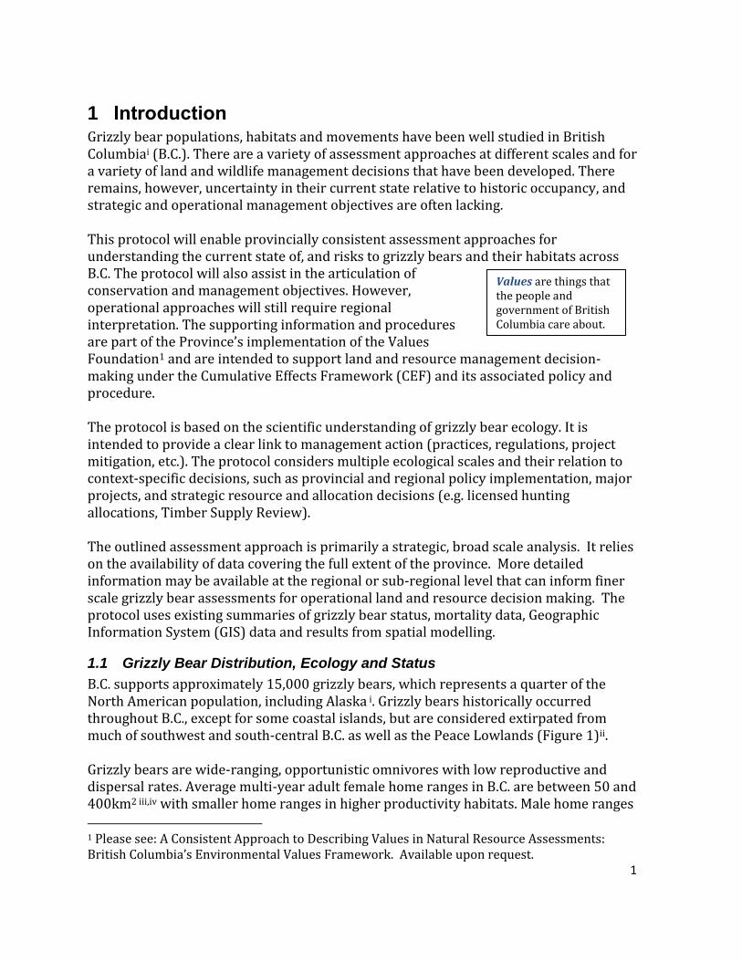
B.C. supports approximately 15,000 grizzly bears, which represents a quarter of the North American population, including Alaska i. Grizzly bears historically occurred throughout B.C., except for some coastal islands, but are considered extirpated from much of southwest and south-central B.C. as well as the Peace Lowlands (Figure 1)ii. Grizzly bears are wide-ranging, opportunistic omnivores with low reproductive and dispersal rates. Average multi-year adult female home ranges in B.C. are between 50 and 400km2 iii,iv with smaller home ranges in higher productivity habitats. Male home ranges
1 Please see: A Consistent Approach to Describing Values in Natural Resource Assessments: British Columbia’s Environmental Values Framework. Available upon request.
Values are things that the people and government of British Columbia care about.
2
Grizzly Bear Population Units B.C.’s grizzly bears exist as a set of interconnected populations, which can be divided into somewhat distinct sub-populations based on bear ecology. For management purposes the province has been divided up into Grizzly Bear Population Units (GBPU) which are a mix of bear biology and management need.
are larger, ranging from 500-2,000km2 with high variation, and overlapping with several females. A British Columbia Grizzly Bear Species Accountv (in revision) summarizes information on grizzly bear biology, ecology and status in B.C.
Figure 1. Status of grizzly bears within the Province's Grizzly Bear Population Units (GBPU).
1.1.1 Conservation threats
Threats to grizzly bears are characterized in the context of ecological risk, where risk to grizzly bears is defined as the probability of ongoing population decline and range reduction. This probability is related to the density of reproductive female grizzly bears (as an indicator of births), mortality and population fragmentation (as an indicator of isolation). When empirical data on grizzly bear vital rates are unavailable, metrics of mortality risk, potential density and fragmentation can be based on landscape condition. For example, when information on female density is lacking (as for some
Landscape Units To assess mortality and habitat at the landscape scale the Province’s Landscape Units are used. These units are analogous to the home range size of a female grizzly bear.
parts of B.C.), habitat availability and forage productivity can be used as a surrogatevi. The effect of habitat on population viability is less well understood than the effect of landscape security on mortality; however, effective, productive habitat supports higher grizzly bear densitiesvi. Habitat and mortality interact; mortality is highest where people and grizzly bears overlap. The scientific rationale for each component and associated indicators are
discussed in more detail in the knowledge summaryvii. Five grizzly bear areas of British Columbia are recognized as Critically Endangered(3), Endangered(1) and Vulnerable(1) under a recent global status review produced by the International Union for Conservation of Nature (IUCN). Federally, grizzly bears are listed as a “species of special concern” in Schedule 3 of the Federal Species at Risk Act2. Under this Act, the grizzly bear’s decline to threatened status would necessitate a national recovery plan and would prohibit activities that harm grizzly bears. Similarly, provincial legislation and regulation provides explicit and implicit direction about sustaining grizzly bears and their habitats, including the:
B.C. Environmental Assessment Act (BC EAA)- Major Project approval and environmental sustainability through Project certification requirements;
Forest and Range Practices Act (FRPA)– Forestry and Range approval and conservation area designations, including Wildlife Habitat Areas and Specified Areas under the Identified Wildlife Management Strategy;
Land Act – land use plan orders containing direction specific to grizzly bears; and
Wildlife Act –associated policies and procedure regarding grizzly bear harvest.
The Province’s Grizzly Bear Conservation Strategy summarizes direction for the management for grizzly bears to “maintain in perpetuity the diversity and abundance of grizzly bears and the ecosystems on which they depend throughout British Columbia” and “to improve the management of grizzly bears and their interactions with humans”3. The grizzly bear policy summary provides a detailed list of all legal and non-legal objectives4.
2 Species at Risk Public Registry. Accessed April 8, 2015: http://www.registrelep-sararegistry.gc.ca/species/default_e.cfm
3 MOELP (Ministry of Environment Lands and Parks). 1995. A future for the grizzly: British Columbia grizzly bear conservation strategy. Accessed Jan 25, 2012: http://www.env.gov.bc.ca/wld/grzz/grst.html
Components, and Functions & Processes Components are the important structural elements and attributes of the value or its environment that can be assessed to describe its condition. Functions & Processes are the energetic processes that define the components and can be either supporting (e.g. species dispersal) or disturbing (e.g. mortality) and can be caused by natural events (e.g. berry production) or human events (e.g. lethal human-bear encounters).
1.1.2 Describing Grizzly Bears
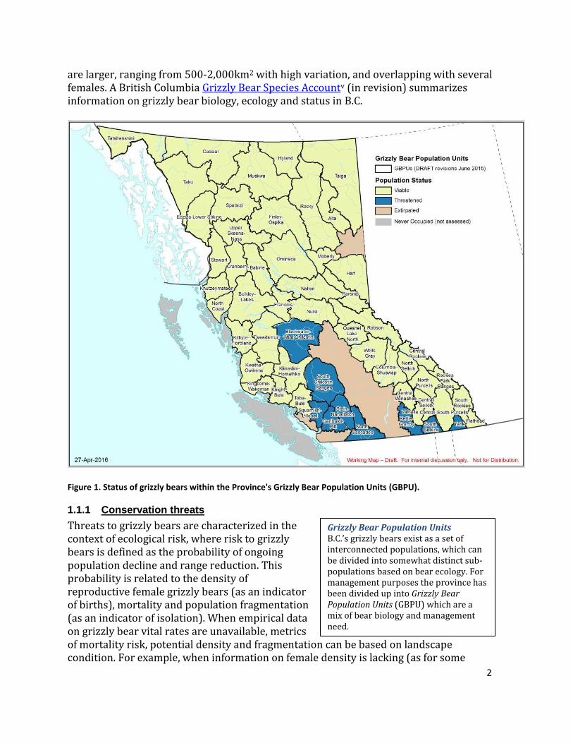
Figure 2. Grizzly bear influence diagram describing the value’s components, and functions & processes. Also shown are the factors considered to assess the risks from threats to grizzly bears.
A variety of different types of diagrams can be used to show important elements and processes in a linked human-ecological systems. Figure 2 is a modified version of a conceptual diagram where all arrows can be read as “influence”.
5
Components, functions and processes that describe the value are presented. Also shown are the factors that influence the functions and processes that were used to determine the condition of those components. These factors were assessed, wherever possible, to evaluate the risk from threats to grizzly bears.
1.1.3 Desired Outcomes
Formally endorsed statements about desired outcomes for grizzly bears provide the context for this assessment , including: 1) the distribution and sustainability of current densities of grizzly bears and their habitats; and 2) achieving habitat restoration and recovery where appropriate. The assessment is structured to evaluate risks to meeting broad provincial objectives and component level regionally-specific objectives. The protocol can also be used to support meeting finer scale-specific objectives within subregions. Based on a review of existing direction for the management of grizzly bears, the following broad objectives are considered for viable GBPUs:
1. At the population scale, ensure grizzly bear populations are sustainable, including managing for genetic and demographic linkage;
2. Continue to manage lands and resources for the provision of sustainable grizzly bear uses as informed by research, inventory and monitoring; and
3. At the landscape scale, sustain and where appropriate, restore the productivity, connectivity, abundance and distribution of grizzly bears and their habitats.
Grizzly bear specific objectives will be weighed and balanced against meeting other economic, social and cultural objectives during statutory decision making under the Province’s CEF. One of the key benefits of the CEF will be the identification and transparency of multi-scale objectives for grizzly bears and their habitats before and after land and resource allocation decision making.
The state of grizzly bear populations in British Columbia ranges from extirpated, through threatened, to expanding and healthy. The Province manages for more than just population viability. Goals vary from maintenance of occupancy and population stability,
Objectives are the desired condition of a value (or component or indicator associated with a value) as defined in legislation, policy, land use plans or agreements with First Nations. Existing objectives are categorized as one of two types: Broad objectives qualitatively describe the
overall desired conditions for a value or component. Typically scientific interpretation is required to identify population and habitat conditions that are consistent with broad objectives and suitable for assessment.
Specific objectives quantitatively describe desired conditions for a value at component or indicator scales. At the indicator scale direct links to management actions can be made. At the component scale a suite of management action may be required to meet the specific component scale objective.
Factors The collection of system elements and processes that can be used to describe functions and processes and the condition of components. Factors are translated into indicators for assessment.
6
resilience and linkage, to objectives for population re-establishment, recovery, and habitat restoration, to the provision of a sustainable licensed harvest or ensuring groups of bears are available for commercial or recreational viewing. In Threatened GBPUs, a process to confirm management direction will be developed to inform specific objectives within those units.
1.1.4 Assessing Risk to Grizzly Bears
Risk statements translate broad objectives to a format suitable for formal risk assessment. A summary of the methods for assessing risk to values is presented in more detail in Morgan et al. 2014. Briefly, risk is the “probability of failing to achieve societal (broad) objectives for a value”. To evaluate broad objectives for grizzly bears, the following risk statements were established for the assessment:
1. Level 1 Risk is the probability of grizzly bear extirpation; and 2. Level 2 Risk is the probability of grizzly bear population and range decline.
Briefly, the assessment considered the following steps: 1. The current status of all factors (ideally all
natural, anthropogenic and climate change threats) that affect risk to the value;
2. Describe, with diagrams and text, the pathways by which factors affect the value;
3. Develop indicators for the main factors; 4. Describe the relationship between risk and the indicator level and describe
associated uncertainty.
For this iteration of the provincial grizzly bear assessment, evaluating the risk statements is done through an interpretation of the cumulative risk associated with each of the factors considered. Further, each of the indicator risk relationships can be treated as a hypothesis and is informed by existing science and monitoring, and identifies further investigation that could be done to better inform the risk relationships. This version of the assessment focused on steps 1 to 3. Future assessment will refine step 4, the risk assessment. For this application a simple flag approach is used where if a critical reference point, or benchmark, is exceeded then the factor is considered to be potentially contributing to risk to meeting the broad objective.
Assessing Natural Resource Systems in Cumulative Effects Assessment The ability of British Columbians to derive environmental, social and economic benefits from the land base is dependent on the condition of the natural resource system. The natural resource system is comprised of the ecological system that provides natural resources and the socio-economic system that contribute to the extraction, delivery, and processing of natural resources from which we derive benefits.
Cumulative effects assessment requires consideration of the condition of the components of natural resource systems, and this in turn requires assessment of system function and the influential processes that affect components over time.
Benchmarks Reference points that support interpretation of the condition of an indicator or component. Benchmarks are based on our scientific understanding of a system, and may or may not be defined in policy or legislation.
7
2 Protocol
2.1 Overview
The protocol is composed of a set of core indicators, and supplemental indicators and indices that are modeled to capture different aspects of grizzly bear ecology and link to general management actions (Figure 3). Metrics describe the specific aspect of the system being measured. The indicators and indices are designed to inform a range of resource management decisions. The core indicators are the primary flags for identifying potential sources of risk to grizzly bears. The supplemental indicators and indices are intended to provide more detail and contextual information for informing decisions. The protocol is intended to provide a provincial standard for assessing grizzly bears, be repeatable and periodically updated. Further, it is intended to be a reference for regional or sub-regional assessment, however, different data sets can be used depending on availability. Similarly the techniques for generating metrics regionally and sub-regionally may depend on the skills and tools available for a specific application. The protocol is also intended to highlight areas of concern for grizzly bear conservation. However, in some cases locating industrial activities in highly impacted areas may result in better outcomes for grizzly bears. For example, front country areas may already be somewhat compromised for supporting bears, or may have infrastructure (e.g. gates) and capacity for promoting grizzly bear conservation (e.g. presence of conservation officers) that can mitigate impacts from proposed human activities. Factors affecting grizzly bears are divided into two components: population and habitat. At the population unit scale (GBPU), indicators are related to grizzly bear population status and mortality rates. At the finer landscape scale (LU), population metrics and indices are related to mortality issues including secure natal areas, quality food sites and human presence, and the density of hunters. The habitat component is considered at the LU and uses forage availability as its indicator, as well as identifying areas of existing habitat protection. A similar diagram is included in Appendix I, but also includes data source and rollup information relevant to the technical assessment. Each of the indicators and indices has the following structure:
Type- Core, supplemental or index; Scientific Context - An overview of the scientific basis for the indicator;
Indicators, Indices & Metrics Indicators describe the factors of the system that are being measured, such as grizzly bear mortality. Indices are a collection of indicators (used as contextual information). Metrics are the specific measurement used (e.g. percent females that have died in a population), and are related to achieving some level of management performance or a specific objective.
8
Management Context - An overview of the different management decisions that could be informed by the indicator;
Indicator/Model Overview –A general description of the indicator/model (model methods are presented in appendices), the specific rationale for the indicator is provided in knowledge summary;
Data Sources; Reporting Strata; Flags; and Validation– Field based projects and existing data sets that were used in the
development of the indicator or model. As well, data that can be used to validate model results.
A detailed listing of Indicators and key reference points, data sources and metadata is provided in Appendix II.
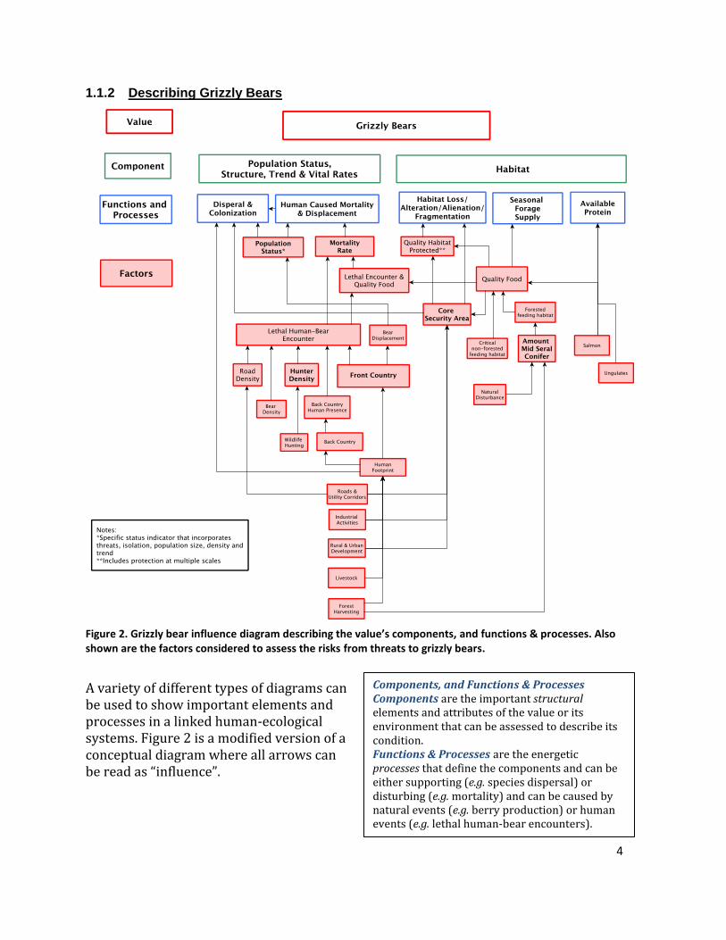
Figure 3. Flow chart outlining components, indicators, metrics, flags, indexes and management actions. Yellow hued boxes designate population component-related factors and green designates habitat components.
9
2.2 Spatial Strata Used in Assessment
Risk to grizzly bears is assessed at two spatial scales: GBPU (sometimes subdivided by Wildlife Management Units (WMU), Limited Entry Hunting (LEH) Zones, and park) and Landscape Units (LU). Assessment results are summarized at the LU polygon level for ease of interpretation and to assist with integrating indicators for presentation.
2.2.1 Grizzly Bear Population Units (GBPUs)
Across much of the province, grizzly bear sub-populations are not isolated units, but form one large population. GBPUs are used for conservation and management, but only a few reflect actual biological populations. Similarly WMU and the LEH Zones are used to capture aspect of bear ecology, but are primarily intended for management purposes, such as setting grizzly bear harvest allocations in some regions. At the GBPU/WMU/LEH scale, assessments characterize risk to the abundance and distribution of grizzly bears within each unit and attempt to reflect regional variation in population management and grizzly bear population ecology.
2.2.2 Landscape Units (LUs)
LUs represent a finer scale and are analogous to the scale of one to several annual female home ranges depending on the size of the landscape unit and quality of the habitat. Habitat and mortality risk indicators can be calculated for each LU and scaled up to allow inference about effects at either a biological population or GBPU/WMU/LEH management scale.
2.3 Spatial Units Used in Assessment
The following spatial units support the assessment of potential risk to grizzly bears.
Area of Grizzly Bear Occupancy
Assessments are required where grizzly bears are known to occur in B.C. (Figure 1).
Grizzly bear population unit (GBPU)
Assessments characterize risk to the abundance and distribution of grizzly bears within a population management unit.
Grizzly bear population units are used for conservation and management, but only a few reflect biological populations.
Wildlife Management Units/Limited Entry Hunt units
Grizzly bear abundance are estimated for each occupied WMU in B.C. Grizzly bear harvest is commonly set by GBPU/WMU/LEH and varies by region.
Landscape Units
Habitat, abundance, and mortality indicators are calculated for each LU.
10
The distribution of secure and risky LUs allows inference about effects at the GBPU/WMU/LEH scale and could provide insights into risk to biological populations.
Grizzly bear forage and habitats
The protocol considers information on habitat abundance and productivity: o At the provincial scale, multi-season habitat capability is calculated using
Broad Ecosystem Inventory maps (BEI), with the exclusion of large water bodies, and ice/glaciers.
o For finer scale application, the distribution of winter, spring, summer and fall habitats, based on TEM or PEM or the direct mapping of stand level habitats can be considered.
o Availability and accessibility of salmon within LUs and at the stream reach scale where available can be used to identify high value protein sites.
o Ungulate and small mammal protein is not considered at this time due to lack of a suitable provincial inventory. Ungulate data is however being investigated for future iterations of the Provincial assessment and it is recommended that ungulate biomass be included in finer scale assessments where available.
Cumulative Effects Reporting Units
The CE reporting units – used to inform regional cumulative effects decision-making. These are analogous to Timber Supply Areas (TSA), Land and Resource Management Plan (LRMP) Areas, or Districts. These reporting units are used to develop Values Report Cards (VRC), for example.
3 Grizzly Bear Metrics
3.1 Grizzly Bear Population Component
3.1.1 Population Status – Core Indicator
Scientific Context State of the Environment reporting presents a summary of the conservation status of grizzly bear populations in B.C.viiiby GBPU. The status assessment was based on estimated population size and the difference between an ideal habitat carrying capacity, excluding human influence, and the current amount of available habitat and extent of human presence. If the population estimate was less than 50% of the ideal then it was considered threatenedix. The B.C. government has adopted the NatureServe population ranking methodology as its approach to assigning species and population status5. The Province is in the process
5 B.C. Conservation Data Centre. Accessed April 8, 2015: Accessed December 11, 2017: http://www.env.gov.bc.ca/cdc/methods.html
11
of updating the status of grizzly bear populations according to NatureServe methods. Under NatureServe methodology criteria for identifying a threatened population includes existing or future threats, population size, population trend, and genetic isolation. A grizzly bear population under human pressure that is declining in numbers, (even if still a minimum viable size) would be a candidate for listing as vulnerable (i.e. equivalent to current threatened designation)x. Further, population fragmentation increases risk of extirpation for isolated sub-populations resulting from demographic and genetic processes.xi Risk increases as isolation increases. Female isolation is the first and most significant risk for grizzly bears, stage of human-caused risk. The highest conservation risks occur when both females and males become isolated from the contiguous meta-population. Female isolation is currently being used as a standard for whether to assess a brown/grizzly bears sub-population or not by the International Union for Conservation of Nature’s (IUCN) Species Survival Commission (SSC). Evaluating female bear isolation is also part of the Provincial re-evaluation of grizzly bear status.
Management Context Decisions related to:
Population recovery planning
Indicator
Population Status
Data Sources
Provincial population (GBPU) status
Reporting Strata
Grizzly Bear Population Unit (GBPU). LU assigned as “Threatened” or “Viable” depending on majority overlap with
GBPU. If there is more than one GBPU overlapping then the “riskiest” status is applied.
Scientific Context Humans are the major cause of mortality in most grizzly bear population units and the majority of human-caused mortality occurs near human occupied areas or roadsxxviii. Bears die at a disproportionate rate when they are close to active roads and people who
12
use the roads are armed. Mortality may occur from mistaken identity kill, human-bear conflict (self-defence kill, management control kill, landowner defence-of-life and property), illegal reported harvest, or vehicle collisions.
Management Context Decisions related to:
Limiting grizzly bear mortality. Grizzly Bear Harvest Management Procedure (under the Wildlife Act) identifies the maximum allowable human-caused mortality for grizzly bear for a defined area, and sets the limit of no more than 30% of this mortality being female bears6 (averaged over a five year allocation period).
Any relevant land use decision that could impact mortality for grizzly bears, including access, regulating hunters (all hunters), education, presence of conservation officers, etc.
Indicator
Bears by sex/year/age/cause – maximum 6% (level varies by unit) total human caused per year.
o female and all bear mortality level o past mortality limit performance
Data Sources
Compulsory inspection data
Reporting Strata
At a minimum GBPU, but could also be defined at the WMU or LEH and National Park.
Extrapolated to the LU level, where LU is assigned a pass or fail depending on overlap (>10%) with a failed mortality polygon, for allowable hunting areas.
Flags The flag is by management unit and is triggered if any allocation period (2004-2006, 2007-2011, 2012-2016) is above the regionally specific mortality limit for all bears or for females only. A unit can flag for no trigger to a total of six possible combinations (if limit violated for both females and all bears for all of the three allocation periods). This will be distinguished as to mortality in open versus closed hunting areas. The map is presented at the management unit scale; however LUs are used for generating the final Provincial roll up (see below).
Validation
TBD
6 Ministry of Environment. 2007. British Columbia Grizzly Bear Harvest Management Procedure Manual. Accessed March 9, 2016: http://www.elp.gov.bc.ca/wld/documents/grizzlybear_harvest_mgmt_proc_2007.pdf.
Scientific Context Current knowledge about bear density is limited. Some populations have been measured; others are estimated based on a regression model that relates landscape-scale factors to the known densitiesxii. These model-based estimates are reviewed and sometimes revised by regional wildlife managers based on local knowledge. Lower densities are a conservation concern whether occurring naturally or resulting from historical effects. Bear densities are typically reported by the GBPU/WMU/LEH/Park administrative unit. Management to population targets is common in adjacent jurisdictions (Alberta and United States (US)). In B.C., no province-wide population targets have been established.
Management Context Decisions related to:
Population recovery planning Estimating historic range occupancy Current population density Establishing licensed hunting allocations Conservation management.
For this assessment, the indicator is used to flag areas with low densities that could be a management concern.
Indicator
Density Estimate - density (bears/1,000km2)
Data Sources
Provincial density estimate25
Reporting Strata
At a minimum GBPU, but could also be defined at the WMU or LEH and National Park.
Bear numbers are extrapolated to the LU using overlapping density and LU area
Flags
Abundance: o Bear Density => 10/1000km2 (lower risk) o Bear Density < 10/1000km2 (higher risk; flagged)
Validation
Population studies. Density estimates derived from field-based DNA studies.
14
3.1.4 Road Density – Supplemental Indicator
Scientific Context Studies have found that most known grizzly bear deaths lie within 500 m of a road or other corridor xiii. Although grizzly bears avoid busy roadsxiv, resource roads with fewer vehicles attract some individuals because of food availability (naturally regenerated or seeded vegetation or carrion), for security from dominant bears, and as travel routesxv. Grizzly bears that are active close to roads usually have a higher risk of human-caused mortalityxvi. Since roads and traffic can alter bear behaviour in complex ways that vary by bear gender and dominance, some demographic groups may experience higher road-related mortality risk than othersxvii. Grizzly bears near roads die from hunting, mistaken identity kills, human-bear conflict and illegal kills; mortality rate is high close to open roads when people who use the roads are armedxviii. Most human-bear conflicts are also near access routes. Collisions with vehicles also kill bearsxix. As road density increases, grizzly bear mortality risk increases, habitat avoidance increases, and populations can declinexx, although nearby areas of high quality secure habitat potentially reduce the impact of high road density at a population scalexxi. Female grizzly bears use an area with lower road density than is available over the landscape, suggesting that they select a home range to minimize roadsxxii. With high road densities, secure grizzly bear habitat can shrink to isolated islands surrounded by a matrix of hazards to the extent that bears do not use areas with high road densityxxiii. Determining a road density threshold for population stability is challenging because of the variety of factors that affect habitat use and mortality, including the distance to human populations, attractiveness of habitat to humans, and human behaviour. Road densities above 0.75 km/km2 were associated with modeled population decline in an Alberta population, considering female reproductive-state specific survival (females with yearlings had higher mortality)xxiv. This work has been used to establish road density targets of 0.6 km/km2 in areas managed for conservationxxv, and of 0.75km/km2 in areas managed for long-term stability. Consistent with this level, adjacent B.C./US trans-border sub-populations have increased in a region where road density in a female home range averages 0.39 km/km2 and decreased where density averaged 0.9 km/km2xxvi. Several studies have recommended thresholds of 0.6 km/km2, and planning processes in B.C., Alberta and the US have used these recommendationsxxvii.
Management Context Decisions related to:
Managing human access – road densities, road closures Managing attractants – right of ways (Hydro lines, pipeline corridors), dumps,
camp management, access to salmon, hunter regulation for managing ungulate kills, etc.
Minimizing bear mortality resulting from negative encounters with humans.
15
Indicators Primary Indicator
Total length of roads divided by the total LU area (km/km2)
Data Sources Road Density: B.C. Consolidated Roads layer: representing a composite from DRA, FTEN, TRIM,
OGC, and RESULTS25 In-block roads, transmission, pipelines, rail
Scientific Context Human access to grizzly bear habitat, and subsequent human behaviour in grizzly bear habitat, is the main reason for declines in grizzly bear populations throughout North Americaxxviii. In the past decade, all-terrain vehicles, global positioning systems and Google Earth have increased accessibility everywhere. Increased risk of human-caused mortality can decrease survival to reproduction, and ultimately, decrease population productivityxxix. The effects of roads are complex, and the magnitude of the effect of roads on grizzly bears varies with several factors, including road density, road location in relation to good quality habitat, road characteristics, traffic patterns, human activities, and grizzly bear age, gender, experience and behaviourxxx. Essentially, where bears and people overlap in space and time, risk of grizzly bear mortality increases, and potentially cause population declines. Core security areas are defined as areas that have adequate habitat with a minimum of human use (after Gibeau et al. 2001, Morgan 2011). They are large enough to accommodate a female grizzly bear’s daily foraging requirements. The integrity of the security area is sensitive to the extent and spatial arrangement of developments including roads, settlements, recreation areas and industrial areas. Appendix IV describes the technical process for identifying secure core areas.
16
Management Context Decisions related to:
Managing human access – road densities, road closures Managing attractants – right of ways (Hydro lines, pipeline corridors), dumps,
camp management, access to salmon, hunter regulation for managing ungulate kills, etc.
Minimizing bear mortality resulting from negative encounters with humans. Hunter education and regulations – “real men use pepper spray”
Indicators
Proportion of capable secure core in patches ≥10km2, within the capable portion of the Landscape Unit.
Data Sources
BEI Capability Ratings Road Density/ Secure Core Analysis (Appendix IV)
o 500m buffers on select human disturbance are also excluded from Secure Core: mining, oil & gas, utility ROWs, agricultural, urban, urban mixed (Appendix III)
Reporting Strata Summarized to landscape Unit.
Flags – For Information
Percent of secure core in LU. Flag is classed as: o 1: ≥ 60% Capable Core (lower risk) o 2: < 60% Capable Core (higher risk; flagged)
Validation Compulsory inspection data.
3.1.6 Front country – Core Indicator
Scientific Context A human-pressure index (see Appendix V) integrates roads, assumed level of road use, human populations, and land type to predict both road density and possible usexxxi. The index is used to differentiate what would be considered front and backcountry areas. Grizzly bears have different interactions with people depending on if the interaction occurs in the front or backcountry. In the backcountry, grizzly bears may be attracted to anthropogenic food sources associated with recreational or industrial camps. Destination sites, such as remote fishing lodges, hunting camps, off-road vehicle cabins and camps, equestrian camps, hiking and backpacking, berry picking, bear viewing lodges, and many other activities and sites, draw people into remote areas and increase human density within bear habitat. Heli-fishing and heli-skiing can bring people into otherwise secure - roadless and high quality habitat - areas. Most research on the
17
potential impacts of human presence in grizzly bear habitat has been road-related, but studies have documented impacts of human use away from roads.xxxii Mortality risk depends on attractant management. Private land is monitored in US conservation strategies. Risk increases as the proportion of rural private land increases. Uncertainty for this indicator is high, due to variability in attractant management and its application as proactive versus reactive. Private land is addressed in US grizzly bear conservation strategies. The front country is defined by urban and rural landscapes include both relatively high human density and grizzly bear attractants in the form of livestock, livestock carcasses, livestock feed, fruit trees, human food/garbage and grain. Bears tend to be absent in urban areas, due to historic human-bear conflict, so these areas do not increase mortality risk to the same extent unless there are anthropogenic attractants along the urban interface. Rural agricultural landscapes essentially provide good quality habitat with high human access, and hence can act as sink habitatxxxiii. In these areas, human-grizzly bear conflicts can lead to defence-of-life-and-property and management killsxxxiv. Grizzly bear density and probability of population persistence decrease as number of livestock increasexxxv. Management strategies, including attractant management (e.g., rapid removal of livestock carcasses, electric fencing) reduces risk of conflict.
Management Context Front Country decisions related to:
Managing attractants – right of ways (Hydro lines, pipeline corridors), dumps, camp management, access to salmon, hunter regulation for managing ungulate kills, etc.
Education for private land – fruit trees, garbage, etc. Managing human access – road densities, road closures, livestock management
on public lands, etc. Managing livestock attractants – (e.g., rapid removal of carcasses, electric fencing
livestock) reduces risk of conflict Managing livestock areas (husbandry practices) Minimizing bear mortality resulting from negative encounters with humans.
Back Country decisions related to: Managing attractants –access to salmon, hunter regulation for managing
ungulate kills, etc. Major project permit requirements, best management practices Minimizing bear mortality resulting from negative encounters with humans.
Indicator Front Country/Back Country designation:
Front Country Landscape Units are defined by: o Human pressure indexfunction of:
Human population size; Travel time on roads, and
18
Land cover 5 classes:
Class 1- Travel time from cities ≤1 hour (Very High Encounter Class)
Class 2- Travel time from cities 1-2 hours (High Encounter Class)
Class 3- Travel time from cities >2 hours, but travel time from high-use road ≤ 1 hour (Moderate Encounter Class)
Class 4- Travel time from cities > 2hours, but travel time from high-use road (Low Encounter Class)
Class 5- Travel time from cities or high-use roads > 2 hours and coastal remote watersheds (Very Low Encounter Class)
Classes 1-3 are considered front country Classes 4&5 and coastal remote watersheds are backcountry
Landscape Units are flagged if >20% of the LU is front country.
Data Sources
B.C. Consolidated Roads layer: representing a composite from DRA, FTEN, TRIM, OGC, and RESULTS25
Human populations o Provincial communities/cities and population
Baseline Thematic Mapping (BTM)xxxvi
Reporting Strata
1 hectare raster model output summarized to Landscape Unit.
Flags Front or backcountry
> 20% Front country (higher risk; flagged) ≤ 20% Front country (lower risk; not flagged).
Validation Compulsory inspection data.
3.1.7 Hunter Day Density – Core Indicator
Scientific Context Grizzly bear mortality occurs at a disproportionate rate when they are close to active roads travelled by people carrying firearmsiv,xxviii. Mortality may occur from mistaken identity kill, poaching, be conflict related (self-defense kill, management control kill, landowner defense-of-life and property kill), and vehicle collisions. Data for the density of hunters in the Province are available at the WMU scale and provides a proxy for hunter day density. Hunter day density combined with metrics of human presence identifies areas where there is higher risk of lethal human-bear encounters.
19
Management Context Minimize bear mortality resulting from negative encounters with hunters.
Indicator Average annual hunter day density. Calculated on number of days over 10 year period (2003-2012)/ per year for the occupied portion of the management unit (MU). This density is used to extrapolate to the LU level (ndays/km2)
Data Sources Hunter Questionnaires and Guide Outfitter declarations.
Reporting Strata Wildlife management unit metric summarized to Landscape Unit.
Flags
Relative ranking of average annual hunter day density by Landscape Unit: Low: 0-0.601977 hunter days/km2 (Quartile 1,2) Mod: 0.601978 - 1.508812 hunter days/km2 (Quartile 3) High: > 1.508812 hunter days/km2 (Quartile 4) (flagged)
Validation Non-hunt mortality will be examined in relation to front-country/back-country and both hunting and non-hunting mortality will be examined in relation to hunter day density using compulsory inspection data.
3.2 Grizzly Bear Habitat Component
3.2.1 Quality Food – Supplemental Indicator
Scientific Context Grizzly bears are omnivores, with a diet that varies with location and seasonxxxvii. In B.C., coastal and interior grizzly bears have very different foraging behaviour and ecology driven by the availability of salmon. On the coast, the spring diet includes early green vegetation, including skunk cabbage, at low elevations. Grizzly bears follow receding snow up avalanche chutes and return to lower slopes for summer berries and salmon runs. They focus on spawning salmon until late fall. Grizzly bear productivity on the coast increases with the availability of salmon and with terrain ruggedness, and decreases with coniferous tree cover. In the interior, early spring diet includes roots and emerging vegetation. Grizzly bears then prey on ungulates at their calving grounds. They focus on berries through summer and fall, supplemented with small mammals, carrion, insects and roots where available. Grizzly bear densities in the interior are best modeled by terrestrial productivity, vegetation cover, terrain ruggedness and human presence. Consistent availability of protein food sources greatly increases habitat quality for grizzly bears and can have a large positive effect on population productivityxxxviii. Grizzly bear density on the coast increases with the proportion of salmon in the dietxxxix. Where
20
people are present, grizzly bears are attracted to anthropogenic attractants including waste dumps, remote camps, fruit trees, etc. For the purposes of this assessment, provincially available data for forage was limited to salmon biomass and high capable areas. Information on ungulate density is intended to be used in the future, as information becomes available. Indicator
Quality Food is identified as: o Salmon biomass by Landscape Unit - Sum of 5 species of salmon kg in LU
over all available time periods > 10,000 kg; and/or o Total Weighted Area of BEI CAPAB1 & 2 in classes 1 (Very High) and 2
(High) > 50% of LU. Quality Food is defined as:
o > 50% of LU is high or very high capability; and/or o Any unit with >10,000kg Salmon biomass.
Data Sources
Salmon escapement data linked to watershed and summarized BEI High and Very High capability
Reporting Strata Summarized to Landscape Unit. Flags – For Information
Yes - high salmon or high capability
No - Not high salmon or high capabilityValidation TBD
Scientific Context Canopy openness is a predictor of berry patches, an important grizzly bear food source, and frequented by bears even outside of berry seasonxl. Mid-seral conifer dominant forestsxli can be dense, have closed canopy and be sub-optimal for forage production. Landscapes with > 30% mid-seral dense coniferous forests should be evaluated for a shortage of forage and included in assessments of suitability, particularly in more sensitive ecological zones. Further, mid-seral condition is tracked when projecting future forest structure and limits to long-term grizzly bear forage supply can be noted.
Management Context Decisions related to:
Managing forage supply – e.g. Timber Supply Review, silviculture, etc.
21
Meeting specific mid-seral objectives in some timber supply areas (e.g. Kalum TSA7).
Indicator
Mid seral is assigned as per NDT/Biogeoclimatic Ecosystem Classification (BEC) forest age criteria from the Biodiversity Guidebook, and further classified for potential forage suitability. 'Low' forage suitability (dark, dense stands with little understory) are considered as 'mid-seral dense conifer'
BEC Zones are distinguished as either High or Moderate sensitivity: o High: CWH, ICH, ESSF, SBS o Moderate: MS, MH, IDF o Low: (all other BEC Zones)
Data Sources
Vegetation Resources Inventory (VRI) Mid-seral forest classification calculated from the Biodiversity Guidebook 25
Reporting Strata Landscape Unit
Flags
Mid-Seral Conifer ≤ 30% in High or Moderate BEC zones (or Low sensitivity BEC Zone) in a landscape unit (low risk)
Mid-Seral Conifer > 30% for select BEC Zones in a landscape unit (high risk) (flagged)
Insufficient Data: VRI gap ≥ 10% of BEC Zone in LU
Validation
Grizzly bear food studies and habitat occupancy studies.
3.2.3 Habitat Protection – Supplemental Indicator
Scientific Context At a coarse scale, Broad Ecosystem Inventory (BEI) units can provide an estimate of habitat capability for abundance of seasonal food. At a 1:250,000 scale, BEI has been used to rate grizzly bear habitat capability and suitability across the province into six classes (very high-1, high-2, moderate-3, low-4, very low-5, nil-6)xlii. At a finer scale (1:20,000 or sometimes 1:50,000), Terrestrial Ecosystem Mapping (TEM) or Predictive Ecosystem Mapping (PEM) can
Habitat Suitability and Capability Capability is defined as the ability of the habitat, under the optimal natural (seral) conditions for a species to provide its life requisites, irrespective of the current condition of the habitat. Suitability is defined as the ability of the habitat in its current condition to provide the life requisites of a species.” xlii
22
provide more precise information. Conservation areas provide some level of habitat protection or restrict some human activity and include provincial parks, national parks, wildlife management areas, visual quality areas, etc. (see Appendix II: 'Meta Protected' Tab for a full list of categories used in this assessment).
Management Context Decisions related to:
Conservation management
Indicators
Percent area of very high and high habitat in conservation areas as a proportion of very high and high habitat in the assessment unit.
Presence/absence of Grizzly Wildlife Habitat Areas (WHA)/Specified Areas or Coastal Ecosystem Based Management (EBM) areas within an LU.
Data Sources
Consolidated Protected and Restricted Areas Dataset BEI High and Very High capability Provincial Grizzly WHAs, excluding Specified Areas with conditional harvesting Coastal EBM Grizzly areas
Reporting Strata
Landscape Unit
Flags – for information Indicator 1:
Low risk >60% protection; Moderate risk 30-60%; and High risk <30% protected
Indicator 2:
Yes: LU contains >= 0.05% WHA/EBM areas (present) No: WHA/EBM areas absent or < 0.05% (absent)
Validation
TBD
3.3 Indexes
3.3.1 Core Indicator Roll Up – High Flag Index
Scientific Context N/A
23
Management Context The overall condition flag counts up the number of indicators that have failed in a landscape unit providing summary information.
Indicator Individual indicators roll ups where an LU is flagged if:
Population is Threatened or Mortality Rate is Exceeded or Capable Secure Core < 60% or Front country > 20% or High Hunter Day Density (>1.5) or BEC Mid-Seral Dense Conifer >30%
o A maximum of six flags are counted. An additional map presents a binary representation of pass/fail (for any indicator) for each Landscape Unit.
Reporting Strata
Landscape Unit
Flags LUs are scored 0 to 6 based on the number of individual indicators that are flagged. If one or more core indicators are flagged, then the rollup flag is triggered. A list is provided (up to 6) of applicable indicators:
Scientific Context Combines front country with areas of high hunter density days to highlight areas of human presence and higher proportion of hunters.
Management Context
See individual indicator’s management context.
Index Combines:
Average Annual Hunter Day Density
24
Front country
Data Sources
See individual metrics
Reporting Strata
LU scale.
Flags
Both Front country > 20% of LU and high average annual hunter day density (high risk)
All other areas (lower risk).
Validation
Compulsory inspection data.
3.3.3 Lethal Encounter with Food Index
Scientific Context The index refines the lethal encounter with the occurrence of quality food.
Management Context
See individual indicator’s management context.
Index Combines:
Lethal encounter index Quality food
Data Sources
See individual metrics
Reporting Strata
LU scale.
Flags
Front country > 20% of LU and high average annual hunter day density and quality food (high risk)
All other areas (lower risk).
Validation
NA
25
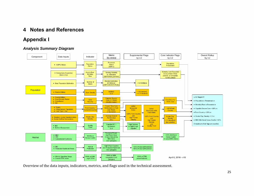
4 Notes and References
Appendix I
Analysis Summary Diagram
Overview of the data inputs, indicators, metrics, and flags used in the technical assessment.
26
Appendix II
Summary Spreadsheet for Indicators, Data Inputs, Assessment Summary Fields, and Metadata for classification of Protected/Restricted Areas, Land Use/Human Disturbance, Ownership, and Road Sources/Use Classification.
Excel sheet provided as a separate document.
27
Appendix III
Derivation of a Consolidated Landbase and Human Disturbance Dataset
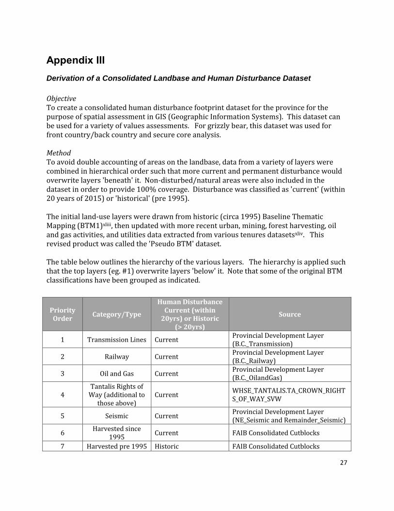
Objective To create a consolidated human disturbance footprint dataset for the province for the purpose of spatial assessment in GIS (Geographic Information Systems). This dataset can be used for a variety of values assessments. For grizzly bear, this dataset was used for front country/back country and secure core analysis. Method To avoid double accounting of areas on the landbase, data from a variety of layers were combined in hierarchical order such that more current and permanent disturbance would overwrite layers 'beneath' it. Non-disturbed/natural areas were also included in the dataset in order to provide 100% coverage. Disturbance was classified as 'current' (within 20 years of 2015) or 'historical' (pre 1995). The initial land-use layers were drawn from historic (circa 1995) Baseline Thematic Mapping (BTM1)xliii, then updated with more recent urban, mining, forest harvesting, oil and gas activities, and utilities data extracted from various tenures datasetsxliv. This revised product was called the 'Pseudo BTM' dataset. The table below outlines the hierarchy of the various layers. The hierarchy is applied such that the top layers (eg. #1) overwrite layers 'below' it. Note that some of the original BTM classifications have been grouped as indicated.
Priority Order
Category/Type
Human Disturbance Current (within
20yrs) or Historic (> 20yrs)
Source
1 Transmission Lines Current Provincial Development Layer (B.C._Transmission)
2 Railway Current Provincial Development Layer (B.C._Railway)
3 Oil and Gas Current Provincial Development Layer (B.C._OilandGas)
4 Tantalis Rights of
Way (additional to those above)
Current WHSE_TANTALIS.TA_CROWN_RIGHTS_OF_WAY_SVW
5 Seismic Current Provincial Development Layer (NE_Seismic and Remainder_Seismic)
6 Harvested since
1995 Current FAIB Consolidated Cutblocks
7 Harvested pre 1995 Historic FAIB Consolidated Cutblocks
28
For further description of the BTM Land Use Classifications, please see the Appendix II spreadsheet, 'meta Development' Tabxlv. Discussion
Although portions of the province have revised BTM, full coverage of the province was only available in version 1 (circa 1995). This provided the basis for the natural/non-disturbed and some historical disturbance.
There was discussion as to adjusting the order of layers, for example that harvesting (with the probability of re-growth) should be placed lower in the hierarchy, below mining and urban disturbance which are more permanent.
Seismic lines are quite extensive in the north-east, and were included in this version of the dataset, however, in many cases they may be less-permanent on the landscape. A fuller understanding of seismic line effects will help advise whether or not they should be included.
Crown tenure polygons may represent only a general tenure area where activity may be permitted, but where the actual disturbance ‘footprints’ are unknown. This includes range tenures, mineral tenures, and agricultural tenures. These types of broad tenure areas, where actual disturbance is unknown, were excluded xxii.
While the use of road buffers was considered, it would have added considerable processing time and potential data processing issues. Roads were analysed separately.
Future runs of the compilation may want to re-consider the hierarchy and inclusion or exclusion of particular layers.
8 Mining Current Provincial Development Layer (B.C._Mining) and BTM 1
9 Urban Current Provincial Development Layers(B.C._Urban) and BTM 1
19 Forest Land N/A BTM 1 (Old Forest, Young Forest, Burned)
20 Range Lands N/A BTM 1
29
Appendix IV.
Core Security Area Model
Objective The objective of this model is to identify areas of secure core habitat capable for grizzly bears (see Grizzly Bear Knowledge Summary Section 3.3.1 vi ). For the purpose of this spatial analysis, secure core areas are defined as areas that are roadless and in patches ≥10 km2. Capable habitat is identified in Broad Ecosystem Inventory (BEI) mappingxlvi, and excludes major water, ice and glacial features. The following 500m buffers on select human disturbance are also excluded from the secure core: mining, oil and gas, utility Rights of Way, agricultural, urban, and urban-mixed use areas. Harvest cut blocks and seismic lines were not included. Method The general steps for determining capable secure habitat were as follows. Details are provided below and illustrated in Figure 3.
1. Calculate road density (raster) for 'open' roads and utilities in order to identify the 'roadless' areas (Figures 3a and 3b).
2. Smooth the 'roadless' areas to eliminate long, narrow 'peninsulas' and select only resulting secure core areas ≥10km2 (Figures 3c, 3d and 3e).
3. Further refine by removal of non-capable areas and select human disturbance to create final capable secure core polygons (Figure 3f).
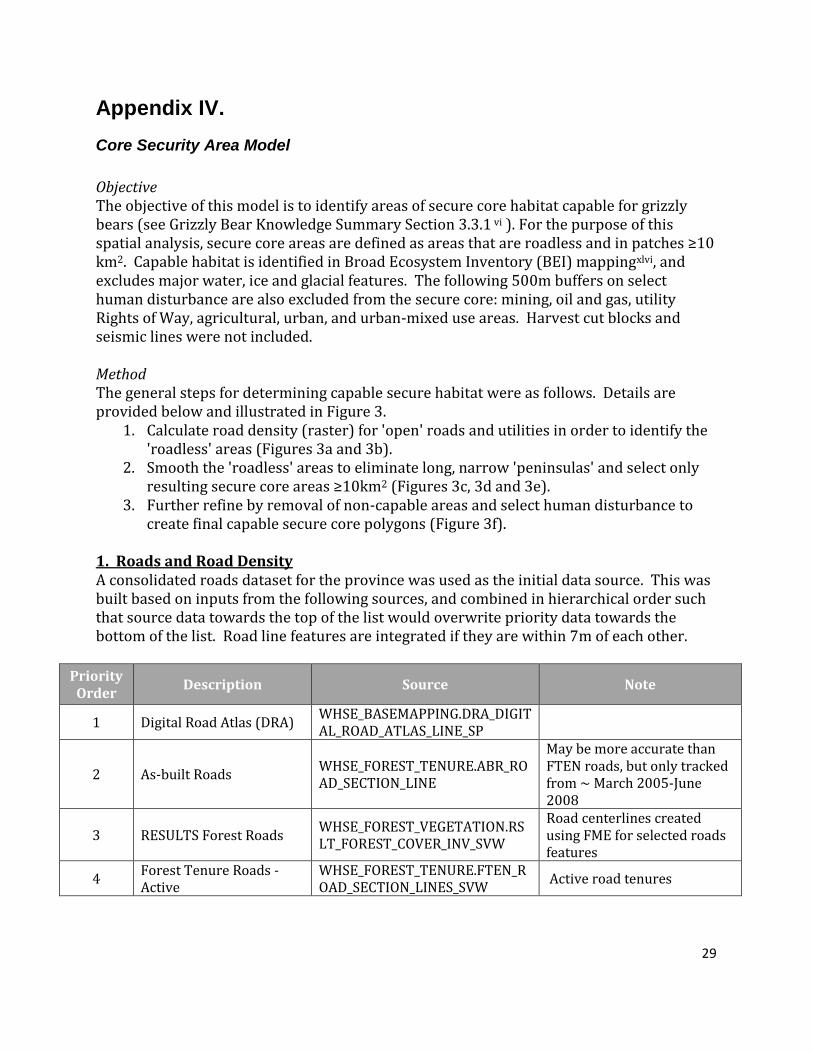
1. Roads and Road Density A consolidated roads dataset for the province was used as the initial data source. This was built based on inputs from the following sources, and combined in hierarchical order such that source data towards the top of the list would overwrite priority data towards the bottom of the list. Road line features are integrated if they are within 7m of each other.
Priority Order
Description Source Note
1 Digital Road Atlas (DRA) WHSE_BASEMAPPING.DRA_DIGITAL_ROAD_ATLAS_LINE_SP
For further description of the roads attributes, please see the Appendix I spreadsheet, ‘meta Roads' Tab xxiii. Ideally for this assessment, only 'open' roads should be considered, as defined in the Recovery Plan For Grizzly Bears in the North Cascades of British Columbiaxlvii: "a road without restriction on motorized vehicle use or that receives use by conventional passenger cars or light-duty trucks (note that gated roads that receive use by conventional passenger cars or light-duty trucks are considered “open”)". The provincial roads datasets have limited information tracked as to restrictions and decommissions. The information that is available may not be up-to-date and is inconsistent between datasets. However, to meet the 'open roads' definition as best as possible, roads were excluded where the attributes were shown as restricted or overgrown (see Appendix 1, 'meta Roads' Tab for a breakdown of available road attributesxxiii). Major utility lines (transmission, pipeline, and rail) were also included. An example of a combined open roads and utilities dataset is shown in Figure 3a. There was a deliberate decision not to use recreation trails, even though there may be additional impact due to motorized off-road vehicles using trail networks. If a finer scale analysis is conducted, then the use of trails data may be recommended. A Road Density raster was calculated using ArcGIS 10.1 Spatial Analyst to identify roadless areas beyond 500m of road influence. The Line Density tool was used with a neighbourhood search radius of 500m, 30m cell size, and units in square km. Grid cells where density was zero were considered roadless (Figure 3b).
31
Road Density Classes were assigned as follows:
Road Density Class Road Density (km/km2)
0 0 (Roadless)
1 0 to 0.3 km/km2
2 >0.3 to 0.6 km/km2
3 >0.6 to 0.75 km/km2
4 >0.75 to 1.25 km/km2
5 >1.25 to 1.75 km/km2
6 >1.75 to 2.5 km/km2
7 >2.5 km/km2
2. Removal of Peninsulas and Small Areas The resulting roadless areas were further 'smoothed' by removing long-narrow peninsulas or irregular areas. The raster processing methodology was developed for ArcGIS, based on the initial concepts of Andrew Fall (Gowlland Technologies) for Spatially Explicit Landscape Event Simulator (SELES). It involves running two moving windows to calculate cell neighbourhood statistics (Focal Statistics tool in ArcGIS):
1) Identify secondary road effects within a 1km circular window (564m radius). Using Focal Statistics, this is the percent of cells within 1 km2 of each grid cell that are at least 564m from roads. If surrounding cells have more than one percent of secondary road influence, then the cell is insecure. Otherwise, if zero road influence, then the cell is considered fully secure (Figure 3c).
2) Run Focal Statistics to determine the number of fully secure cells within 1 km2 of insecure cells. If there is at least one fully secure cell adjacent, then the cell is secure. If there are no fully secure neighbours then the cell is still insecure, and is filtered out (Figure 3d). Another way to look at this is that the fully secure areas area 'ballooned' out to fill significant adjacent cells. This effectively results in removal of irregular areas.
Finally, these resulting smoothed areas are selected for areas ≥10km2. Areas < 10km2 are filtered out or ignored, to produce the 'Secure Core' layer (Figure 3e). 3. Refine for Capable Habitat The smoothed secure core is further refined to include capable habitat only and exclude 500m buffers on select human disturbance (mining, oil and gas, utility Rights of Way, agricultural, urban, and urban mixed use areas). This uses the Broad Ecosystem Inventory (BEI) selected for capable habitat ratings 1-5 (Very High to Very Low), with exclusion of major water bodies, ice and glacial features from the Baseline Thematic Mapping (BTM). Area is weighted by BEI capable proportion. Note that removal of non-capable areas may split a contiguous area of 'secure core' into smaller portions, and reduce the overall size and contiguity, however fragmented areas are still maintained as overall secure core.
32
Select disturbances (see Appendix II) were buffered by 500m and excluded/erased from the core areas. The final 'Capable Secure Core' is capable habitat in secure core areas > =10km2 (Figure 3f). Figure 3 illustrates the progression from road density to roadless to capable secure core for a sample landscape unit.
33
Fig.3a. Open Roads and Utilities in the Coquihalla Landscape Unit
Fig.3c. Focal Statistics 1 to determine 'Fully Secure' areas
Fig.3e. Classification of Secure Core by size
Fig.3b. Road Density and Roadlessness Classification
Fig.3d. Focal Statistics 2 'ballooning' to add adjacent Secure areas
Fig.3f. Final Capable Secure Core, excluding non-secure, non- capable habitat, and select disturbance.
Figure 3. Progression from Roads to Road Density to Capable Secure Core Habitat using ArcGIS
34
Appendix V
Human Pressure Index
Human population pressure corresponds to the likelihood of encountering humans at a particular location on the landscape. This relates to access (e.g. road type, off-road terrain type), assumed travel rates, and proximity to sizeable human populations. The following is based on concepts proposed by Clayton Apps xxxi. The analysis was prepared by Andrew Fall (Gowlland Technologies) using SELES. The first step of a human pressure index is to determine, for each community, the travel time to every location on the landscape. The landscape is defined by 1 hectare grid cells in a raster environment. Travel time must be computed for (a) every community and (b) for every location in the study area (at least up to some maximum travel time limit). To compute travel time for every community requires that diffusion is initiated in each community in sequence (i.e. one at a time, as opposed to simultaneously). Diffusion spread rate is done as follows:
(i) On roads: at the road type speed limit (Table 1) Off-road: a speed equal to the likely fasted mode of travel for the cover type (often by foot, but perhaps by (often by foot, but perhaps by snowmobile or ATV on land, or by boat or swimming/wading across water). Boat swimming/wading across water). Boat access is assumed only possible when the water body is accessible by water body is accessible by road. Once mode of travel is by foot, it cannot revert to motorized travel (
to motorized travel (
(ii) Table 2).
Table 1. Travel speeds applied by road type (See Appendix II) for provincial scale analysis. More detailed road speed classification can be applied in study areas with higher precision road information.
Road Type Travel speed (motorized) High use 100 kmh Moderate use 50 kmh Low use 25 kmh
35
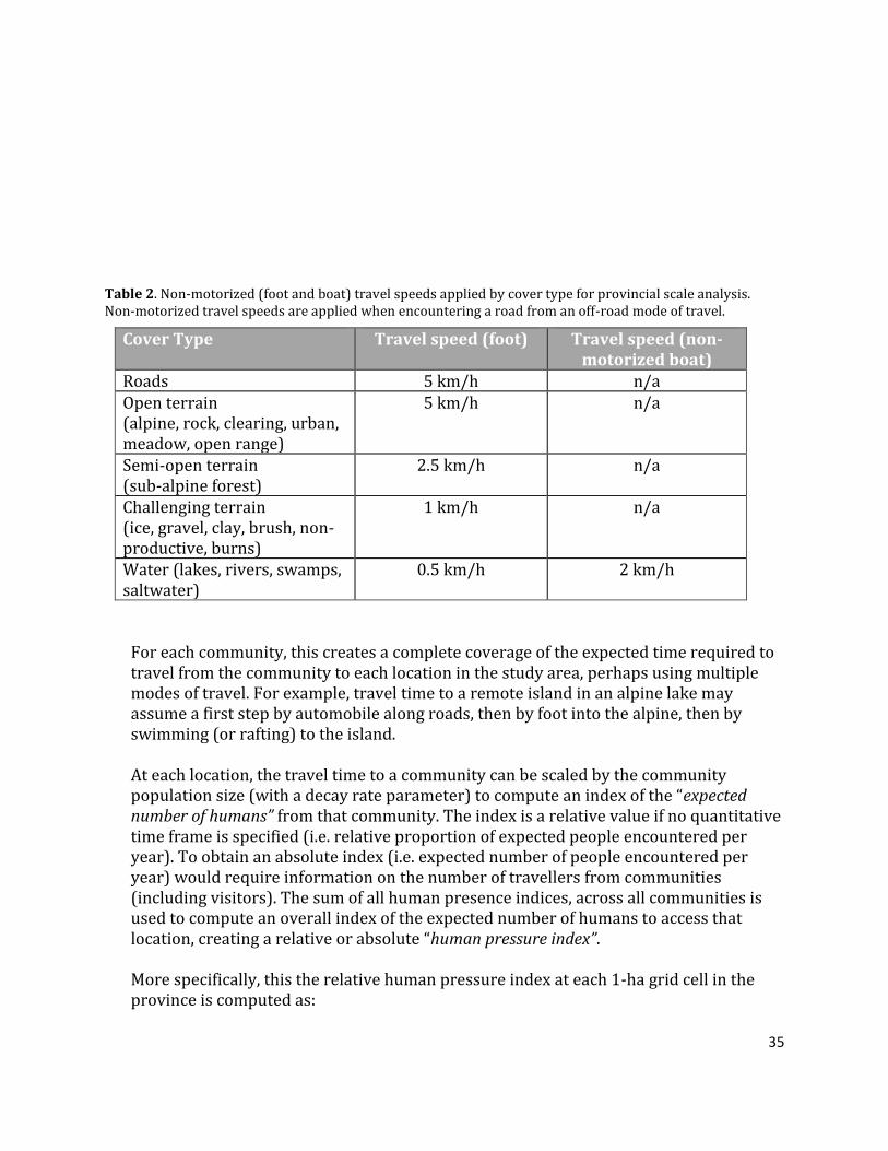
Table 2. Non-motorized (foot and boat) travel speeds applied by cover type for provincial scale analysis. Non-motorized travel speeds are applied when encountering a road from an off-road mode of travel.
Cover Type Travel speed (foot) Travel speed (non-motorized boat)
Roads 5 km/h n/a Open terrain (alpine, rock, clearing, urban, meadow, open range)
For each community, this creates a complete coverage of the expected time required to travel from the community to each location in the study area, perhaps using multiple modes of travel. For example, travel time to a remote island in an alpine lake may assume a first step by automobile along roads, then by foot into the alpine, then by swimming (or rafting) to the island. At each location, the travel time to a community can be scaled by the community population size (with a decay rate parameter) to compute an index of the “expected number of humans” from that community. The index is a relative value if no quantitative time frame is specified (i.e. relative proportion of expected people encountered per year). To obtain an absolute index (i.e. expected number of people encountered per year) would require information on the number of travellers from communities (including visitors). The sum of all human presence indices, across all communities is used to compute an overall index of the expected number of humans to access that location, creating a relative or absolute “human pressure index”. More specifically, this the relative human pressure index at each 1-ha grid cell in the province is computed as:
36
∑𝑝𝑜𝑝(𝑐) ∗ 𝑑𝑡(𝑐,𝑖𝑗)𝑛
𝑐=1
Where ij is the grid cell (row i, column j)
n is the number of communities
pop(c) is the population size of community c
d is the decay rate of human pressure with distance
t(c, ij) is the travel time in hours to grid cell location ij from community c
The current scenarios apply a decay rate parameter d of 0.5 (i.e. human pressure decreases at a rate of 50% per hour of travel time). One limitation of the above approach to human pressure is that it does not consider “attractiveness” of sites. That is, while it can consider the effect of faster travel along trails and open, gentler terrain (i.e. “push factors” from communities towards easier-to-reach locations), it does not consider the “pull factor” of locations that attract humans (e.g. scenic views, remote camp sites, fishing locations) that may draw more human presence compared with other locations of equal travel time. The travel time from cities and high-use roads was further interpreted into five classes:
1: Travel time from cities <= 1 hour 2: Travel time from cities 1-2 hours 3: Travel time from cities > 2 hours, but travel time from high-use road <= 1 hour 4: Travel time from cities > 2 hours, but travel time from high-use road 1-2 hours 5: Travel time from cities or high-use roads > 2 hours
where classes 1-3 are considered front country, and classes 4 and 5 are considered backcountry. This was used as a main indicator for likelihood of human-bear encounter. Data Sources:
B.C. Consolidated Roads layer: representing a composite from DRA, FTEN, TRIM, OGC, and RESULTS25
Human populations o 1:2M city population (2000)25
BTMxlviii
37
References i Grizzly Bear Population Status in B.C. 2012. Environmental Reporting BC.
http://www.env.gov.bc.ca/soe/indicators/plants-and-animals/grizzly-bears.html ii Grizzly Bear Population Status in B.C. 2012.Accessed (June 29, 2015):
http://www.env.gov.bc.ca/soe/indicators/plants-and-animals/grizzly-bears.html iii Tony Hamilton. June 23, 2015. Unpublished data. iv Ciarniello, L.M., M.S. Boyce, D.C. Heard, and D.R. Seip. 2009. Comparison of grizzly bear demographics in
wilderness mountains versus a plateau with resource development. Wildlife Biology 15:247–265 v Gyug, L., Hamilton T., and Austin, M. 2004. Grizzly bear—accounts and measures for managing identified
wildlife. http://www.env.gov.bc.ca/wld/frpa/iwms/accounts.html vi Mowat G, Heard DC, Schwarz CJ 2013. Predicting grizzly bear density in Western North America. PLoS
ONE 8:e82757.Doi: 10.1371/journal.pone.0082757. vii Provincial Grizzly Bear Technical Working Group. 2016. Grizzly Bear Knowledge Summary. (June 30,
2015). 43 pp. viii Grizzly Bear Population Status in BC. 2012. Environmental Reporting B.C. Accessed (June 30, 2015):
http://www.env.gov.bc.ca/soe/indicators/plants-and-animals/grizzly-bears.html ix Hamilton, A.N.. D.C. Heard, and M.A. Austin, 2004. British Columbia Grizzly Bear (Ursus arctos)
Population Estimate. B.C. Ministry of Water, Land and Air Protection, Victoria, B.C. 7pp. x Faber-Langendoen, D., J. Nichols, L. Master, K. Snow, A. Tomaino, R. Bittman, G. Hammerson, B.
Heidel, L. Ramsay, A. Teucher, and B. Young. 2012. NatureServe Conservation Status Assessments: Methodology for Assigning Ranks. Arlington, VA. URL: http : / / connect . natureserve . org / sites / default / files / documents / NatureServeConservation%StatusMethodology Jun12.pdf.
xi Lande R. 1988. Genetics and demography in biological conservation.Science 241:1455-1460; Frankham R, Ballous JD, Briscoe DA. 2002. Introduction to conservation genetics. Cambridge University
Press, Cambridge, UK; WoodroffeR, Ginsberg JR. 1998. Edge effects and the extinction of populations inside protected areas. Science 280:2126-2128.
xii Mowat G, Heard DC, Schwarz CJ 2013. Predicting grizzly bear density in Western North America. PLoS ONE 8:e82757.Doi: 10.1371/journal.pone.0082757.
xiii Wakkinen, W.L., and W.F. Kasworm. 1997. Grizzly bear and road density relationships in the Selkirk and Cabinet–Yaak recovery zones. Idaho Fish and Game, Bonners Ferry, Idaho and U.S. Fish and Wildlife Service, Libby, Montana, USA.; McLellan, B. N. 2015. Some mechanisms underlying variation in vital rates of grizzly bears on a multiple use landscape. The Journal of Wildlife Management 79: 749–765.; Benn B. 1998. Grizzly bear mortality in the Central Rockies Ecosystem, Canada. MSc Thesis, U Calgary, Alberta 163 pp.; Boulanger and Stenhouse 2014 The impact of roads on the demography of grizzly bears in Alberta. PLoS ONE 9(12): e115535., Benn B, Herrero S. 2002. 2002. Grizzly bear mortality and human access in Banff and Yoho National Parks, 1971-98. Ursus 13:213-221.
xiv Mace, R.D., Waller, J.S., Manley, T.L., Lyon, L.J. and Zuuring, H., 1996. Relationships among grizzly bears, roads and habitat in the Swan Mountains Montana. Journal of Applied ecology, pp.1395-1404.; Northrup, J.M., Pitt, J., Muhly, T.B., Stenhouse, G.B., Musiani, M. and Boyce, M.S., 2012. Vehicle traffic shapes grizzly bear behaviour on a multiple‐use landscape. Journal of Applied Ecology, 49(5), pp.1159-1167.
xv Nagy JA, Russell RH. 1978. Ecological studies of the boreal forest grizzly bear (Ursus arctos L.) – annual report for 1977. Canadian Wildlife Service, Edmonton, Alberta, Canada; MacHutchon AG, Mahon T. 2003. Habitat use by grizzly bears and implications for forest development activities in the Kispiox Forest District; final report. Skeena Cellulose Incorporated, Hazelton and B.C. MWLAP, and BCSRM, Smithers; Herrero S, Smith T, DeBruyn TD, Gunther K, Matt CA. 2005. Brown bear habituation to people: safety, risks, and benefits. Wildlife Society Bulletin 33:362-373; Roever C, Boyce MS, Stenhouse BG. 2008. Grizzly bears and forestry1: road vegetation and placement as an attractant to grizzly bears. Forest Ecology and Management 256:1253-1261; Schwarz CC, Cain S, Podruzny S, Cherry S, Frattaroli L. 2010. Contrasting activity patterns of sympatric and allopatric black and grizzly bears. Journal of Wildlife Management 74:1628-1638; Haroldson MA, Gunther KA. 2013. Roadside bear viewing opportunities in Yellowstone National Park: characteristics, trends, and influence of whitebark pine. Ursus 24:27-41.
xvi Johnson et al. 2004; Nielsen SE, Herrero S, Boyce MS, Mace RD, Benn B, Gibeau M, Jevons . 2004.
Modeling the spatial distribution of human-caused grizzly bear mortalities in the Central Rockies Ecosystem of Canada. Biological Conservation 120:101-113; Graham K, Boulanger J, Duval J, Stenhouse G. 2010. Spatial and temporal use of roads by grizzly bears in west-central Alberta. Ursus 21:43-56; Schwartz et al. 2010; Boulanger and Stenhouse 2014.
xvii Boulanger and Stenhouse 2014. The impact of roads on the demography of grizzly bears in Alberta. PLoS ONE 9(12): e115535.
xviii Mattson DJ, Herrero S, Wright RG, Pease CM. 1996. Science and management of Rocky Mountain grizzly bears. Conservation Biology 10:1013-1025. McLellan BN, Hovey FW, Mace RD, Woods JG, Carney DW, Gibeau ML, Wakkinen WL, Kasworm WF. 1999. Rates and causes of grizzly bear mortality in the interior mountains of British Columbia, Alberta, Montana, Washington, and Idaho. Journal of Wildlife Management 63: 911-920; Johnson CJ, Boyce MS, Schwartz CC, Haroldson MA, 2004. Modelling survival: application of the Andersen-Gill model to Yellowstone grizzly bears. Journal of Wildlife Management 68:966-978; Ciarniello LA, Boyce MS, Heard DC, Seip DR. 2007. Components of grizzly bear habitat selection: density, habitats, roads, and mortality risk. Journal of wildlife Management 71:1446-1457; Schwartz et al. 2010; McLellan BN in review. Some mechanism underlying variation in vital rates of grizzly bears on a multiple use landscape. Journal of wildlife Management
xix Gunther KA, Biel MJ, Robison HL. 1998. Factors influencing the frequency of road-killed wildlife in Yellowstone National Park. PP 32-42 in GL Evink (ed) Proceedings of the International Conference on Wildlife Ecology and Transportation, Florida department of Transportation, Tallahassee, Florida; Bertch B, Gibeau M. 2009. Grizzly bear monitoring in and around the Mountain National Parks: mortalities and bear/human encounters 1990-2008. Parks Canada, Lake Louise, Alberta.
xx Kasworm W, Manley T. 1990. Road and trail influences on grizzly bears and black bears in northwest Montana. International Conference on Bear Research and Management 8:79-84; Mace et al. 1996; Apps CS, McLellan BN, Woods JG, Proctor JF. 2004. Estimating grizzly bear distribution and abundance relative to habitat and human influence. Journal of Wildlife Management 68:138-152; Schwartz et al. 2010; Boulanger et al. 2013; Boulanger and Stenhouse 2014; MacHutchon AG, Proctor M. 2015. Management plan for the Yahk and South Selkirk grizzly bear (Ursus arctos) sub-populations, British Columbia. Trans-border Grizzly Bear Project, Kaslo 104 pp.
xxi McLellan, B. N. 2015. Some mechanisms underlying variation in vital rates of grizzly bears on a multiple use landscape. The Journal of Wildlife Management 79: 749–765.
xxii MacHutchon and Proctor 2015. The Effect of Roads and Human Action on Roads on Grizzly Bears and their Habitat. Trans-border Grizzly Bear Project. 12pp. Accessed January 30, 2018: http://www.coasttocascades.org/s/MacHutchon_Proctor_23-Feb- 2015_Effects_of_Roads_on_Grizzly_Bears.pdf
xxiii Mace et al. 1996; Gibeau ML, Herrero S, McLellan BN, Woods JG. 2001. Managing for grizzly bear security areas in Banff National Park and the Central Canadian Rocky Mountains. Ursus 12:121-130; Schwartz et al. 2010
xxiv Boulanger and Stenhouse 2014. The impact of roads on the demography of grizzly bears in Alberta. PLoS ONE 9(12): e115535.
xxv Alberta Grizzly Bear Recovery Plan 2008-2013. 2008. Alberta Sustainable Resource Development, Fish and Wildlife Division, Alberta Species at Risk Recovery Plan #15. Edmonton, AB, 68pp.
xxvi MacHutchon and Proctor 2015. The Effect of Roads and Human Action on Roads on Grizzly Bears and their Habitat. Trans-border Grizzly Bear Project. 12pp. Accessed January 30, 2018: http://www.coasttocascades.org/s/MacHutchon_Proctor_23-Feb- 2015_Effects_of_Roads_on_Grizzly_Bears.pdf
xxvii Mace et al. 1996; Noss RF, Quigley HB, Hornocker MG, Merrill T, Paquet PC. 1996. Conservation biology and carnivore conservation in the Rocky Mountains. Conservation Biology 10:949-963; Alberta Grizzly Bear Recovery Plan 2008-2013. 2008. McLellan BN, Hovey FW. 2001. Habitats selected by grizzly bears in a multiple use landscape. Journal of Wildlife Mangement 65:92-99. B.C. Ministry of Ministry of Environment, Lands and Parks 2000. Environmental trends in B.C. 2000. State of Environment Reporting. Accessed April 30, 2014: http://www.env.gov.bc.ca/soe/archive/reports/93_98_00/enviro-trends2000.pdf; Antoniuk T, Ainslie
B. 2003. CEAMF Study Volume 2: cumulative effects indicators, thresholds, and CEAMF, edited by Salmo Consulting Inc. and Diversified Environmental Services: Prepared for the B.C. Oil and Gas Commission. Muskwa-Kechika Advisory Board.
xxviii McLellan BN. 1990. Relationships between human industrial activity and grizzly bears. International conference on Bear Research and Management 8:57-64; Schoen JW. 1990. Bear habitat management: a review and future perspective. International conference on Bear Research and Management 8:143-154;
Banci V, Demarchi DA, Archibald WR. 1994. Evaluation of the population status of grizzly bears in Canada. International conference on Bear Research and Management 9:129-144; Mattson and Merrill 2002.
xxix Mace et al. 1996, Wakkinen WL, Kasworm WF. 1997. Grizzly bear and road density relationship in the Selkirk and Cabinet-Yaak recovery zones. Idaho Fish and Game, Bonners Ferry, Idaho and US Fish and Wildlife Service, Libby Montana US; Proctor M, Servheen C, Kasworm W, Radandt T. 2008. Habitat security for grizzly bears in the Yahk Grizzly Bear Population Unit of the south Purcell Mts. of southeast British Columbia. Trans-border Grizzly Bear Project, Kaslo, BV, Canada. http://www.transbordergrizzlybearproject.ca; Schwartz CC, Haroldson MA, GC White. 2010. Hazards ffecting grizzly bear survival in the greater Yellowstone ecosystem. Journal of Wildlife Management 74:654-667; Boulanger J, Cattet M, Nielsen SE, Stenhouse G, Cranston J. 2013. Use of multi-state models to explore relationships between changes in body condition, habitat and survival of grizzly bears Ursus arctos horribilis. Wildlife Biology 19:274-288; 2013, Boulanger J, Stenhouse G. 2014. The impact of roads on the demography of grizzly bears in Alberta. PLoS ONE 9(12):e115535
xxx See Table 2 of Appendix 3: MacHutchon and Proctor “The effect of roads and human action of roads on grizzly bear and their habitat”
xxxi Apps, C., B. McLellan, and C. Servheen. 2014. Modeling human accessibility and remoteness to assist grizzly bear population research and cumulative effects assessment. Pages 18 - 22 in Resource Roads in British Columbia: Environmental challenges at a landscape level. Columbia Mountains Institute of Applied Ecology, Revelstoke, B.C., Canada.
xxxiiColeman TCH, Schwartz CC, Gunther KA, Creel S 2013. Influence of overnight recreation on grizzly bear movement and behavior in Yellowstone National Park.Ursus: 101; Cristescu B, Stenhouse GB, Boyce MS 2013. Perception of human-derived risk influences choice at top of the food chain. PLoS ONE 8:1-12.
xxxiiNorthrup et al. 2012. Vehicle traffic shapes grizzly bear behaviour on a multiple‐use landscape. Journal of Applied Ecology, 49(5), pp.1159-1167.
xxxii Gunther KA, Haroldson MA, Frey K, Cain SL, Copeland J, Schwartz CC. 2004. Grizzly bear-human conflicts in the Greater Yellowstone ecosystem, 1992-2000. Ursus 15:10-22; Wilson SM, Madel MJ, Mattson DJ, Graham JM, Merrill T. 2006. Landscape conditions predisposing grizzly bears to conflicts on private agricultural lands in the western USA. Biological Conservation 130:47-59.
USA. Biological Conservation 130:47-59. xxxiiMattson and Merrill 2002. Extirpations of grizzly bears in the contiguous United States, 1850–
2000. Conservation Biology, 16(4), pp.1123-1136; Mowat G, Heard DC, Schwarz CJ 2013. Predicting grizzly bear density in Western North America. PLoS ONE 8:e82757.Doi: 10.1371/journal.pone.0082757.
xxxvi Ministry of Forests, Lands and Natural Resource Operations - GeoBC, Baseline Thematic Mapping
Present Land Use Version 1 Spatial Layer Metadata. Accessed (2015): http://catalogue.data.gov.bc.ca/dataset/baseline-thematic-mapping-present-land-use-version-1-spatial-layer
xxxvii Summarized from Gyug et al. 2004. Grizzly Bear Ursus arctos. Accounts and Measures for managing Identified Wildlife. 21 pp.; Mowat G, Heard DC, Schwarz CJ 2013. Predicting grizzly bear density in Western North America. PLoS ONE 8:e82757.Doi: 10.1371/journal.pone.0082757.
xxxviii Mowat G, Heard DC, Schwarz CJ 2013. Predicting grizzly bear density in Western North America. PLoS ONE 8:e82757.Doi: 10.1371/journal.pone.0082757.
Lausen CL, Gibeau ML, Wakkinen WL, Haroldson MA, Mowat G, Apps , Ciarniello LM, Barclay RMR, Boyce MS, Schwartz CC, Strobeck c. 2012. Population fragmentation and inter-ecosystem movements of grizzly bears in Western Canada and the Northern United States. Wildlife Monographs 180:1-46.
xli Province of British Columbia, 1995. Biodiversity Guide Book. Victoria, British Columbia, Canada. xliiB.C. Ministry of Environment, Lands and Parks. 1999. British Columbia wildlife habitat rating
standards version 2. https://www.for.gov.bc.ca/hts/risc/pubs/teecolo/whrs/assets/whrs.pdf xliii Ministry of Forests, Lands and Natural Resource Operations - GeoBC, Baseline Thematic Mapping
Present Land Use Version 1 Spatial Layer Metadata. Accessed (2015): http://catalogue.data.gov.bc.ca/dataset/baseline-thematic-mapping-present-land-use-version-1-spatial-layer
xliv Cumulative Effects Assessment Provincial Development Layer Documentation, 2015. In-progress/Available upon request. xlv Supplemental: CEFVF_Appendix1_Indicators_Inputs_DataDict_Grizzly_24Sept2015_Phase1.xlsx
xlvii North Cascades Grizzly Bear Recovery Team, 2004. Recovery Plan for Grizzly Bears in the North Cascades of British Columbia. Accessed (2015) http://www.env.gov.bc.ca/wld/documents/recovery/ncgbrt_final.pdf
xlviii Ministry of Forests, Lands and Natural Resource Operations - GeoBC, Baseline Thematic Mapping
Present Land Use Version 1 Spatial Layer Metadata. Accessed (2015): http://catalogue.data.gov.bc.ca/dataset/baseline-thematic-mapping-present-land-use-version-1-spatial-layer