53
Introduction to Introduction to Econometrics Econometrics The Statistical Analysis of Economic (and related) Data
| Date post: | 09-Aug-2015 |
| Category: |
Business |
| Upload: | orion-constellation |
| View: | 60 times |
| Download: | 0 times |
Introduction to EconometricsIntroduction to Econometrics
The Statistical Analysis of
Economic (and related) Data
2
What do economists study?
What is the quantitative effect of reducing class size on
student achievement?
How does another year of education change earnings?
What is the price elasticity of cigarettes?
What is the effect on output growth of a 1 percentage point
increase in interest rates by the Fed?
What is the effect on housing prices of environmental
improvements?
3
How do we answer these questions? Ideally, we would like an experiment
what would be an experiment to estimate the effect of class size on standardized test scores?
But almost always we only have observational (nonexperimental) data.
returns to education cigarette prices monetary policy
Most of the course deals with difficulties arising from using observational data to estimate causal effects:
omitted variables simultaneous causality “correlation does not imply causation”
4
Review of Probability and Statistics(SW Chapters 2, 3) Empirical problem: Class size and educational output
Policy question: What is the effect on test scores (or some
other outcome measure) of reducing class size by one student
per class?
We must use data to find out (is there any way to answer this
without data?)
5
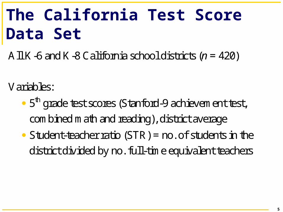
The California Test Score Data Set
All K-6 and K-8 California school districts (n = 420)
Variables:
5th grade test scores (Stanford-9 achievement test,
combined math and reading), district average
Student-teacher ratio (STR) = no. of students in the
district divided by no. full-time equivalent teachers
6
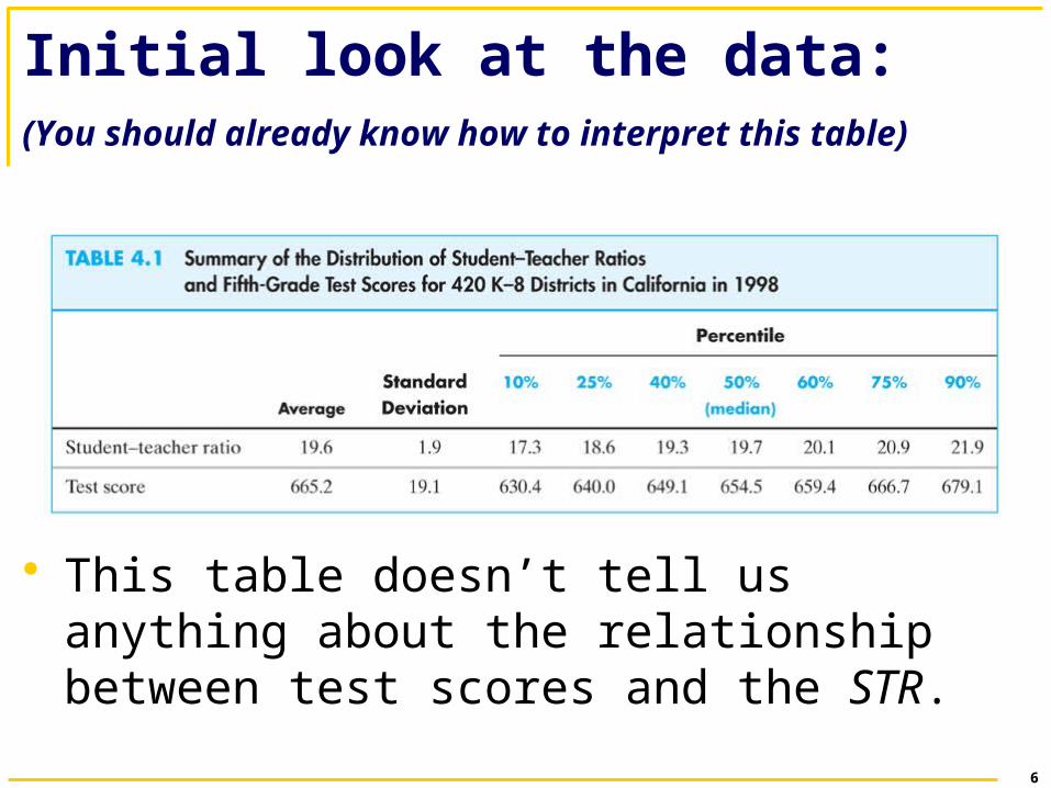
Initial look at the data:(You should already know how to interpret this table)
This table doesn’t tell us anything about the relationship between test scores and the STR.
7
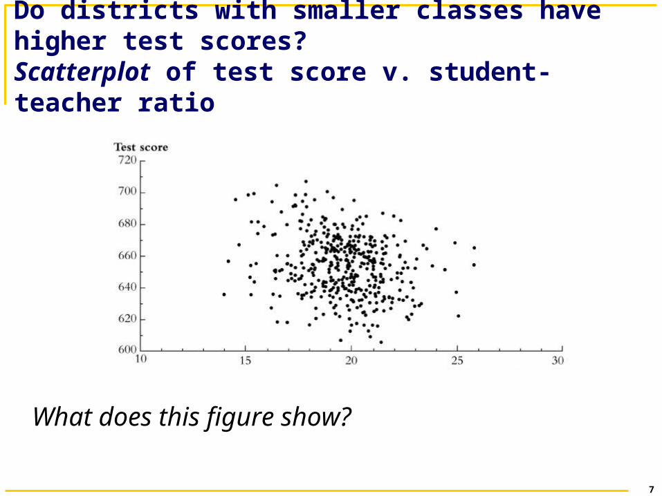
Do districts with smaller classes have higher test scores? Scatterplot of test score v. student-teacher ratio
What does this figure show?
8
How do we answer this question with data?
1. Compare average test scores in districts with low STRs to
those with high STRs (“estimation”)
2. Test the “null” hypothesis that the mean test scores in the
two types of districts are the same, against the
“alternative” hypothesis that they differ (“hypothesis
testing”)
3. Estimate an interval for the difference in the mean test
scores, high v. low STR districts (“confidence interval”)
9
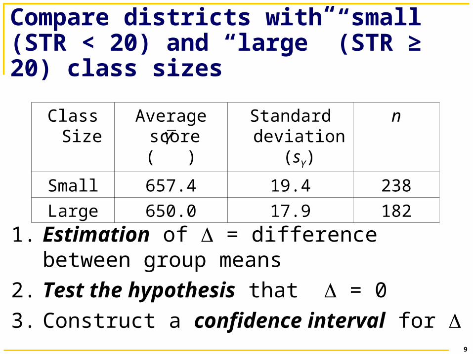
Compare districts with “small” (STR < 20) and “large” (STR ≥ 20) class sizes
1. Estimation of = difference between group means
2. Test the hypothesis that = 0
3. Construct a confidence interval for
YClass Size Average score
( )Standard
deviation (sY)n
Small 657.4 19.4 238
Large 650.0 17.9 182
10
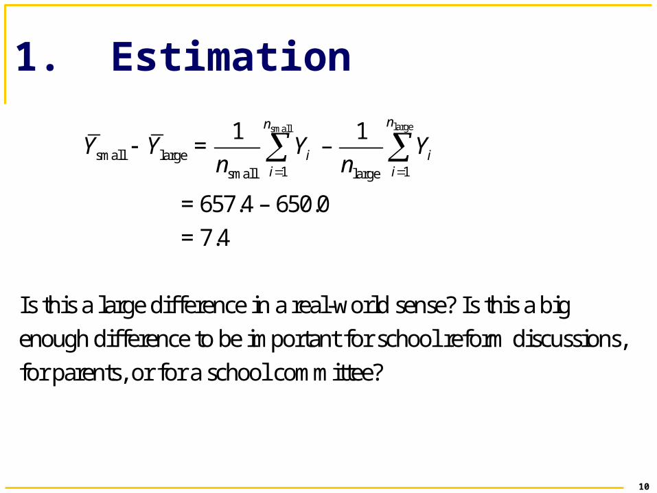
1. Estimation
small largeY Y = small
1small
1 n
ii
Yn
– large
1large
1 n
ii
Yn
= 657.4 – 650.0
= 7.4
Is this a large difference in a real-world sense? Is this a big
enough difference to be important for school reform discussions,
for parents, or for a school committee?
11
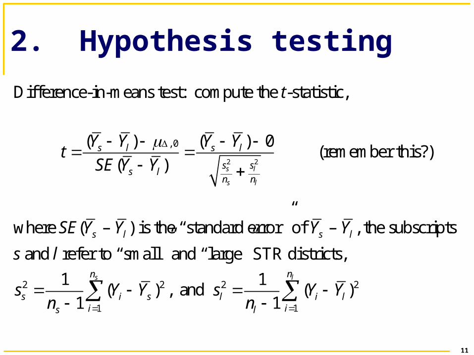
2. Hypothesis testing
Difference-in-means test: compute the t-statistic,
2 2
, 0( ) ( ) 0
( ) s l
s l
s l s l
s ss l
n n
Y Y Y Yt
SE Y Y
(remember this?)
where SE( sY – lY ) is the “standard error” of sY – lY , the subscripts
s and l refer to “small” and “large” STR districts,
2 2
1
1( )
1
sn
s i sis
s Y Yn
, and 2 2
1
1( )
1
ln
l i lil
s Y Yn
12
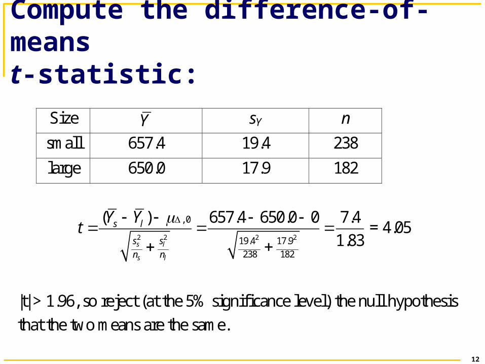
Compute the difference-of-means t-statistic:
Size Y sY n
small 657.4 19.4 238
large 650.0 17.9 182
2 2 2 2
, 0
19.4 17.9
238 182
( ) 657.4 650.0 0 7.4
1.83s l
s l
s l
s s
n n
Y Yt
= 4.05
|t| > 1.96, so reject (at the 5% significance level) the null hypothesis
that the two means are the same.
13
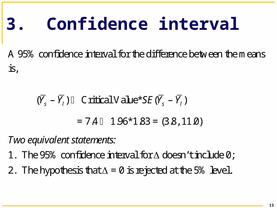
3. Confidence interval
A 95% confidence interval for the difference between the means
is,
( sY – lY ) Critical Value*SE( sY – lY )
= 7.4 1.96*1.83 = (3.8, 11.0)
Two equivalent statements:
1. The 95% confidence interval for doesn’t include 0;
2. The hypothesis that = 0 is rejected at the 5% level.
14
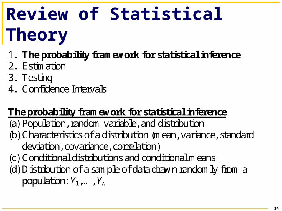
Review of Statistical Theory
1. The probability framework for statistical inference 2. Estimation 3. Testing 4. Confidence Intervals The probability framework for statistical inference (a) Population, random variable, and distribution (b) Characteristics of a distribution (mean, variance, standard
deviation, covariance, correlation) (c) Conditional distributions and conditional means (d) Distribution of a sample of data drawn randomly from a
population: Y1,…, Yn
15
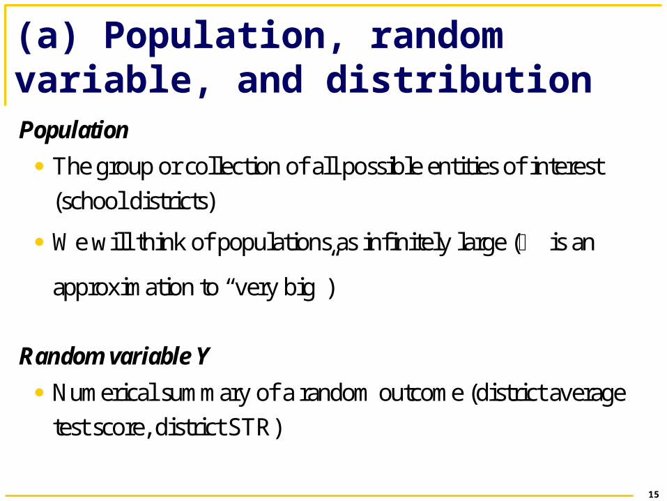
(a) Population, random variable, and distribution Population
The group or collection of all possible entities of interest
(school districts)
We will think of populations as infinitely large ( is an
approximation to “very big”)
Random variable Y
Numerical summary of a random outcome (district average
test score, district STR)
16
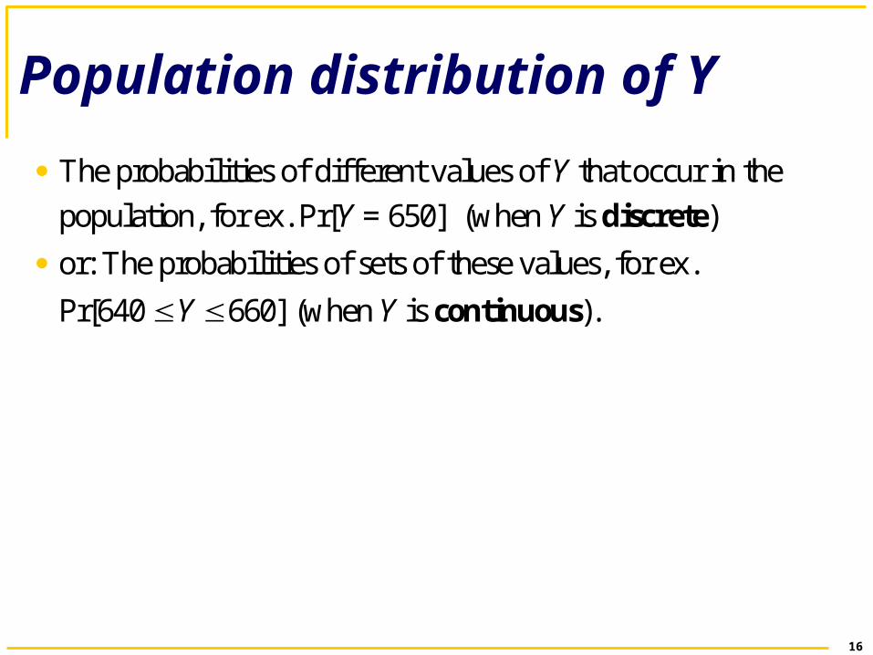
Population distribution of Y
The probabilities of different values of Y that occur in the
population, for ex. Pr[Y = 650] (when Y is discrete)
or: The probabilities of sets of these values, for ex.
Pr[640 Y 660] (when Y is continuous).
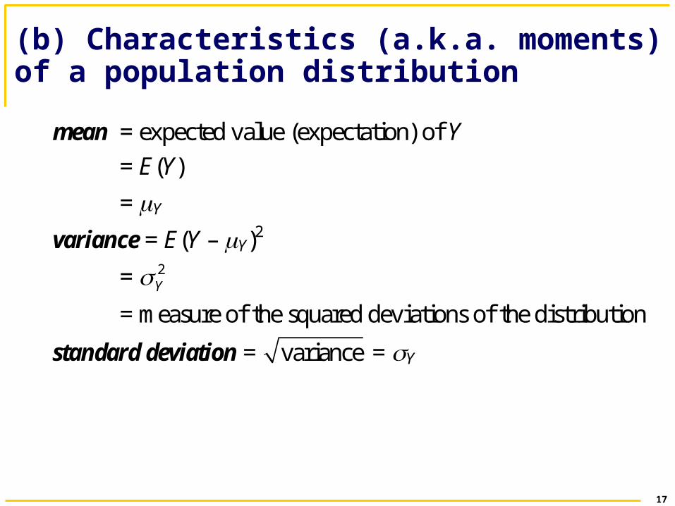
(b) Characteristics (a.k.a. moments) of a population distribution
17
mean = expected value (expectation) of Y
= E(Y)
= Y
variance = E(Y – Y)2
= 2Y
= measure of the squared deviations of the distribution
standard deviation = variance = Y
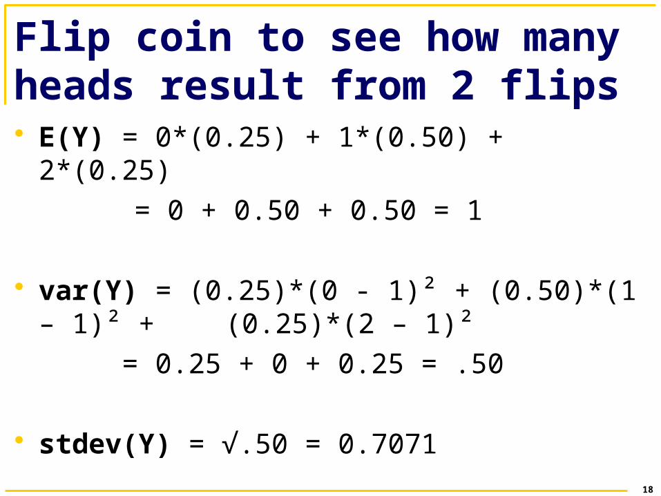
Flip coin to see how many heads result from 2 flips E(Y) = 0*(0.25) + 1*(0.50) + 2*(0.25)
= 0 + 0.50 + 0.50 = 1
var(Y) = (0.25)*(0 - 1)² + (0.50)*(1 – 1)² + (0.25)*(2 – 1)²
= 0.25 + 0 + 0.25 = .50
stdev(Y) = √.50 = 0.7071
18
19
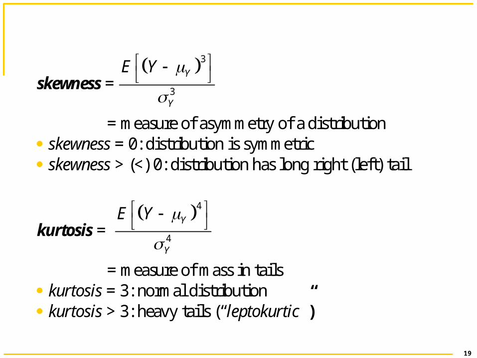
skewness = 3
3
Y
Y
E Y
= measure of asymmetry of a distribution skewness = 0: distribution is symmetric skewness > (<) 0: distribution has long right (left) tail
kurtosis = 4
4
Y
Y
E Y
= measure of mass in tails kurtosis = 3: normal distribution kurtosis > 3: heavy tails (“leptokurtic”)
20
21
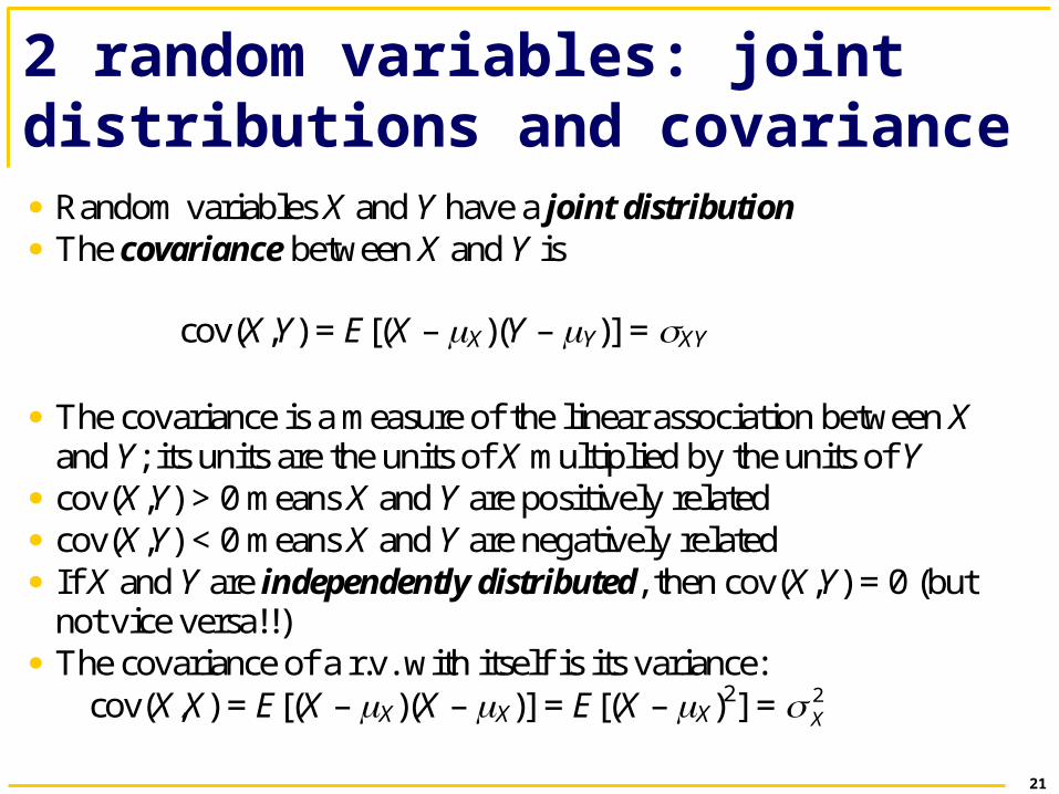
2 random variables: joint distributions and covariance Random variables X and Y have a joint distribution The covariance between X and Y is
cov(X,Y) = E[(X – X)(Y – Y)] = XY
The covariance is a measure of the linear association between X
and Y; its units are the units of X multiplied by the units of Y cov(X,Y) > 0 means X and Y are positively related cov(X,Y) < 0 means X and Y are negatively related If X and Y are independently distributed, then cov(X,Y) = 0 (but
not vice versa!!) The covariance of a r.v. with itself is its variance:
cov(X,X) = E[(X – X)(X – X)] = E[(X – X)2] = 2X
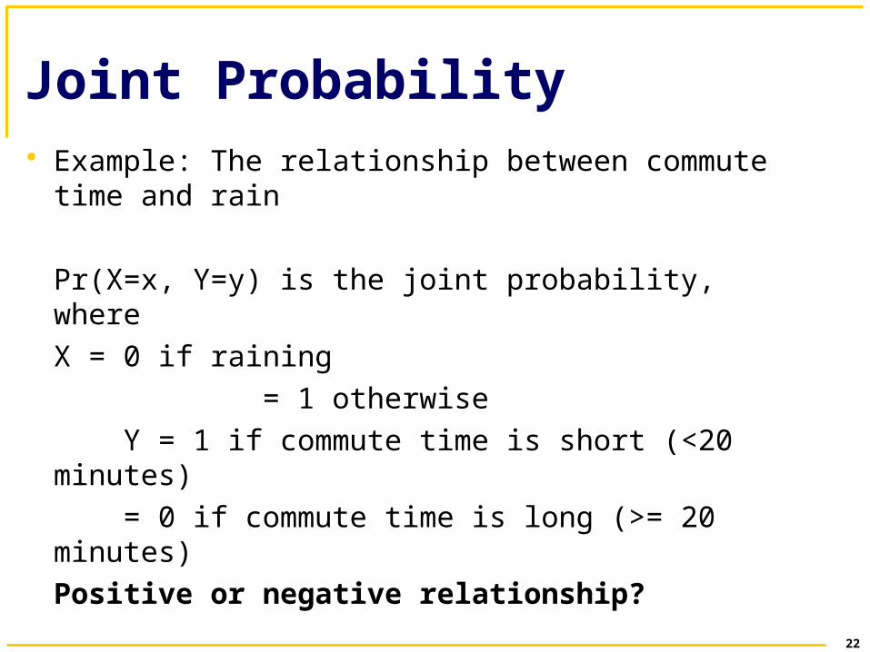
Joint Probability Example: The relationship between commute time
and rain
Pr(X=x, Y=y) is the joint probability, where
X = 0 if raining
= 1 otherwise
Y = 1 if commute time is short (<20 minutes)
= 0 if commute time is long (>= 20 minutes)
Positive or negative relationship?
22
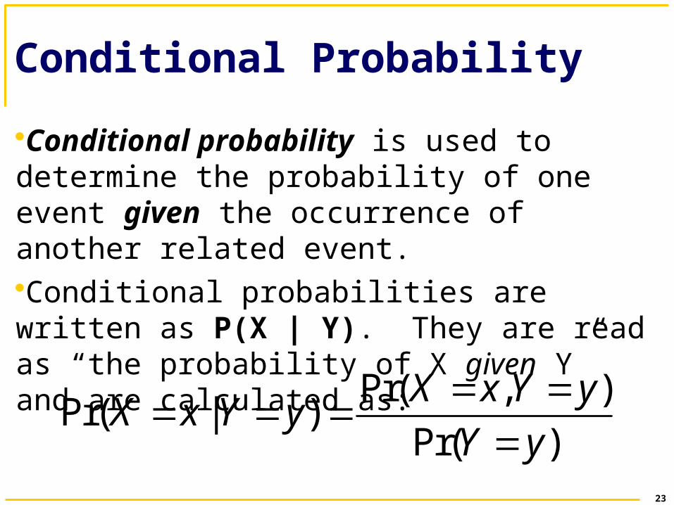
Conditional Probability
Conditional probability is used to determine the probability of one event given the occurrence of another related event.Conditional probabilities are written as P(X | Y). They are read as “the probability of X given Y” and are calculated as:
23
Pr( , )Pr( | )
Pr( )
X x Y yX x Y y
Y y
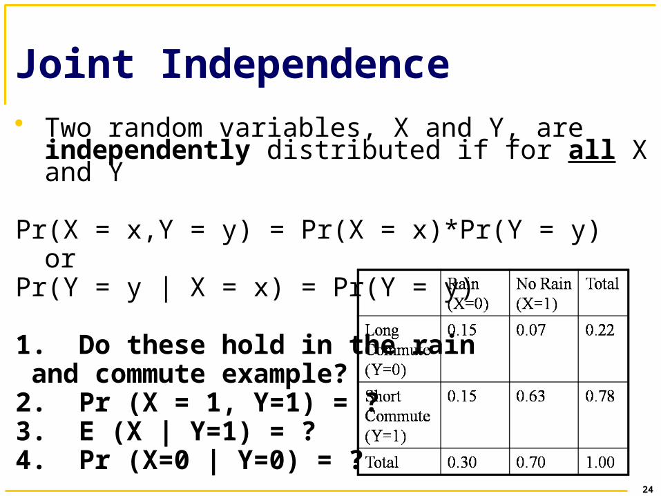
Joint Independence Two random variables, X and Y, are independently
distributed if for all X and Y
Pr(X = x,Y = y) = Pr(X = x)*Pr(Y = y)or
Pr(Y = y | X = x) = Pr(Y = y)
1. Do these hold in the rain and commute example?2. Pr (X = 1, Y=1) = ?3. E (X | Y=1) = ?4. Pr (X=0 | Y=0) = ?
24
25
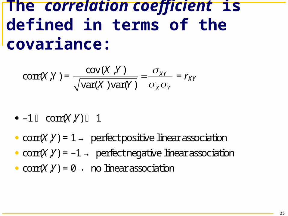
The correlation coefficient is defined in terms of the covariance:
corr(X,Y) = cov( , )
var( ) var( )XY
X Y
X Y
X Y
= rXY
–1 corr(X,Y) 1
corr(X,Y) = 1 → perfect positive linear association
corr(X,Y) = –1 → perfect negative linear association
corr(X,Y) = 0 → no linear association
26
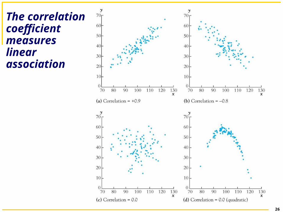
The correlation coefficient measures linear association
27
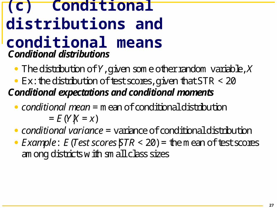
(c) Conditional distributions and conditional means Conditional distributions
The distribution of Y, given some other random variable, X Ex: the distribution of test scores, given that STR < 20
Conditional expectations and conditional moments
conditional mean = mean of conditional distribution = E(Y|X = x)
conditional variance = variance of conditional distribution Example: E(Test scores|STR < 20) = the mean of test scores
among districts with small class sizes
28
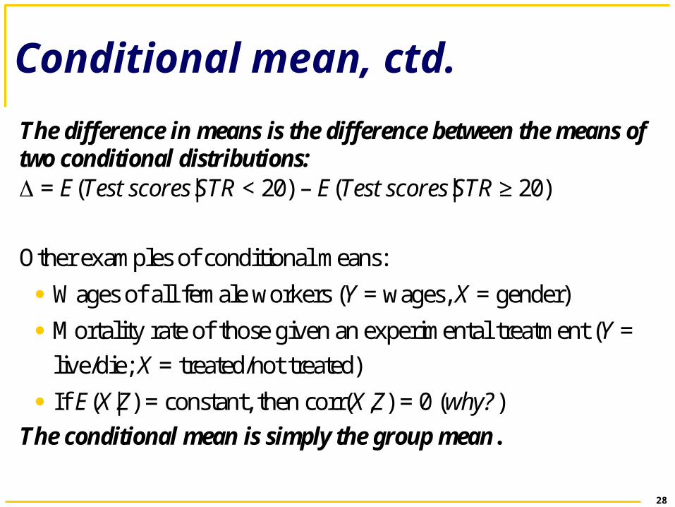
Conditional mean, ctd.
The difference in means is the difference between the means of two conditional distributions:
= E(Test scores|STR < 20) – E(Test scores|STR ≥ 20)
Other examples of conditional means:
Wages of all female workers (Y = wages, X = gender)
Mortality rate of those given an experimental treatment (Y =
live/die; X = treated/not treated)
If E(X|Z) = constant, then corr(X,Z) = 0 (why?)
The conditional mean is simply the group mean.
29
(d) Distribution of a sample of data drawn randomly from a population: Y1,…, Yn
We will assume simple random sampling
Choose an individual (district, entity) at random from the
population
Notation
The data set is (Y1, Y2,…, Yn), where Yi = value of Y for the ith
individual (district, entity) sampled
30
Distribution of Y1,…, Yn under simple random sampling Because individuals #1 and #2 are selected at random, the
value of Y1 tells us nothing about Y2. Therefore: Y1 and Y2 are independently distributed Y1 and Y2 come from the same distribution, that is, Y1, Y2
are identically distributed → Under simple random sampling, {Yi}, i = 1,…, n, are independently and identically distributed (i.i.d.).
We want to draw statistical inference about the characteristics of a population using a sample of data from that population.
31
1. The probability framework for statistical inference
2. Estimation
3. Testing
4. Confidence Intervals
Estimation
Y , the sample mean, is an estimator of the population mean.
(a) What are the properties of Y ?
(b) Why should we use Y rather than some other estimator?
Y1 (the first observation)
maybe unequal weights – not simple average
median(Y1,…, Yn)
The answers lie in the sampling distribution of Y .
32
(a) The sampling distribution of YY is a random variable, and its properties are determined by the
sampling distribution of Y
The individuals in the sample are drawn at random. The values of (Y1,…, Yn) are random. Functions of (Y1,…, Yn), such as Y , are random: had a
different sample been drawn, they would have taken on a different value.
The distribution of Y over different samples is called the sampling distribution of Y .
The mean and variance of the sampling distribution are E(Y ) and var(Y ).
33
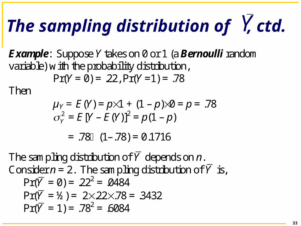
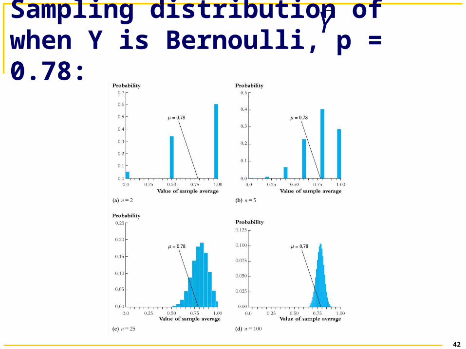
The sampling distribution of , ctd. YExample: Suppose Y takes on 0 or 1 (a Bernoulli random variable) with the probability distribution,
Pr(Y = 0) = .22, Pr(Y =1) = .78 Then
µY = E(Y) = p1 + (1 – p)0 = p = .78 2Y = E[Y – E(Y)]2 = p(1 – p)
= .78 (1–.78) = 0.1716
The sampling distribution of Y depends on n. Consider n = 2. The sampling distribution of Y is,
Pr(Y = 0) = .222 = .0484 Pr(Y = ½) = 2.22.78 = .3432 Pr(Y = 1) = .782 = .6084
34
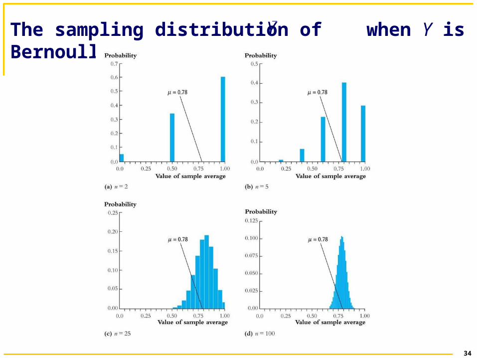
The sampling distribution of when Y is Bernoulli (p = .78):
Y
35
Things we want to know about the sampling distribution: What is the mean of Y ?
If E(Y ) = = .78, then Y is an unbiased estimator of What is the variance of Y ?
How does var(Y ) depend on n? Does Y get closer to as n gets larger?
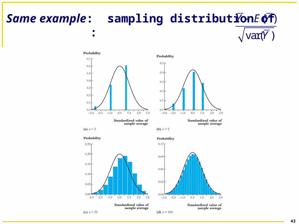
Law of Large Numbers: Y is a consistent estimator of Y – appears bell shaped for n large…is this generally true?
In fact, Y – is approximately normally distributed for n large (Central Limit Theorem)
36
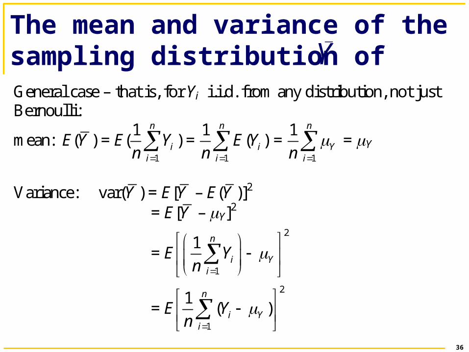
The mean and variance of the sampling distribution of YGeneral case – that is, for Yi i.i.d. from any distribution, not just Bernoulli:
mean: E(Y ) = E(1
1 n
ii
Yn ) =
1
1( )
n
ii
E Yn =
1
1 n
Yin
= Y
Variance: var(Y ) = E[Y – E(Y )]2
= E[Y – Y]2
= E2
1
1 n
i Yi
Yn
= E2
1
1( )
n
i Yi
Yn
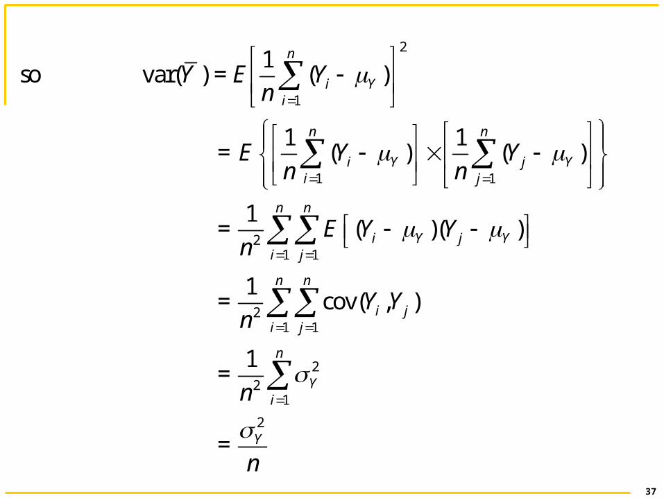
37
so var(Y ) = E2
1
1( )
n
i Yi
Yn
= 1 1
1 1( ) ( )
n n
i Y j Yi j
E Y Yn n
= 2
1 1
1( )( )
n n
i Y j Yi j
E Y Yn
= 2
1 1
1cov( , )
n n
i ji j
Y Yn
= 22
1
1 n
Yin
= 2Y
n
38
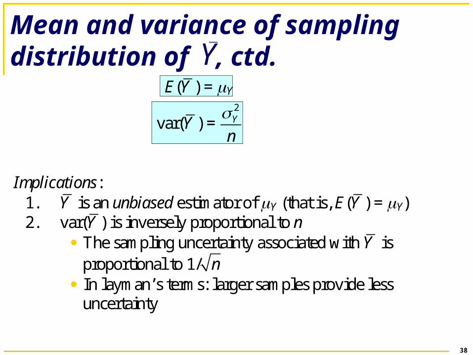
Mean and variance of sampling distribution of , ctd.
E(Y ) = Y
var(Y ) = 2Y
n
Implications: 1. Y is an unbiased estimator of Y (that is, E(Y ) = Y) 2. var(Y ) is inversely proportional to n
The sampling uncertainty associated with Y is proportional to 1/ n
In layman’s terms: larger samples provide less uncertainty
Y
39
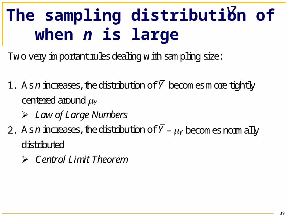
The sampling distribution of when n is large
Y
Two very important rules dealing with sampling size:
1. As n increases, the distribution of Y becomes more tightly
centered around Y
Law of Large Numbers
2. As n increases, the distribution of Y – Y becomes normally
distributed
Central Limit Theorem
40
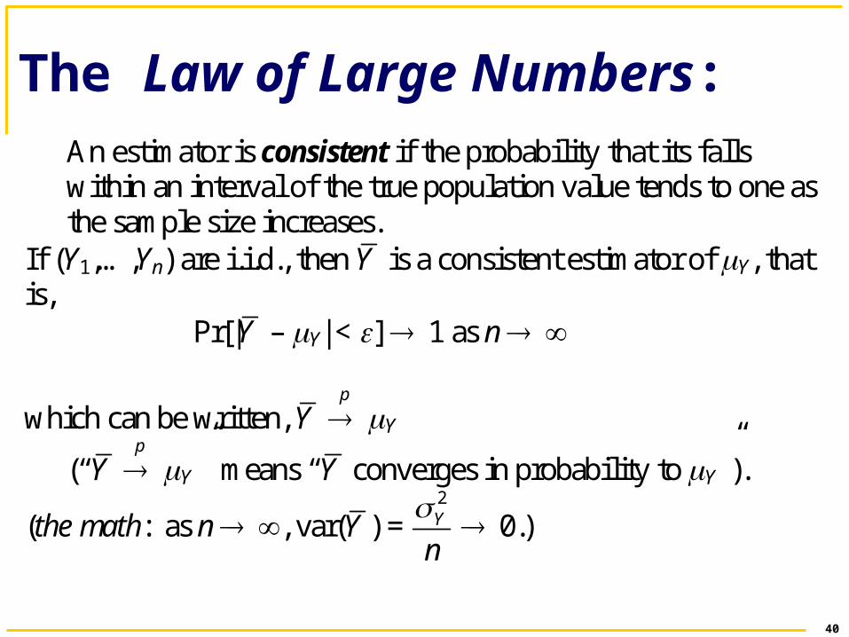
The Law of Large Numbers: An estimator is consistent if the probability that its falls within an interval of the true population value tends to one as the sample size increases.
If (Y1,…,Yn) are i.i.d., then Y is a consistent estimator of Y, that is,
Pr[|Y – Y| < ] 1 as n
which can be written, Y p
Y
(“Y p
Y” means “Y converges in probability to Y”).
(the math: as n , var(Y ) = 2Y
n
0.)
41
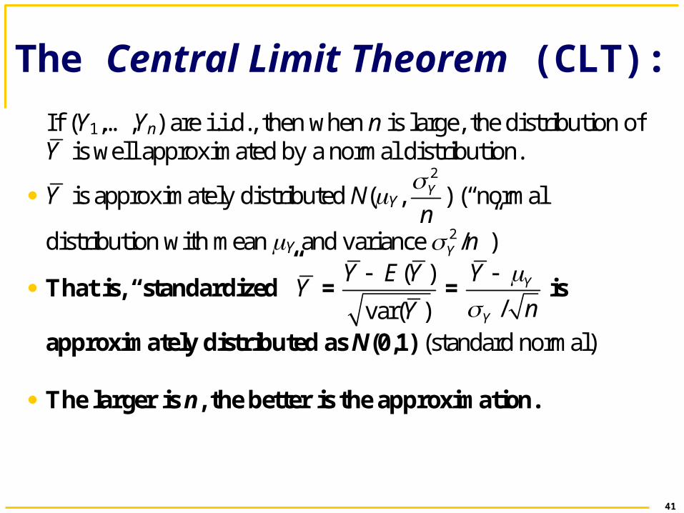
The Central Limit Theorem (CLT):
If (Y1,…,Yn) are i.i.d., then when n is large, the distribution of Y is well approximated by a normal distribution.
Y is approximately distributed N(Y, 2Y
n
) (“normal
distribution with mean Y and variance 2Y /n”)
That is, “standardized” Y = ( )
var( )
Y E Y
Y
=
/Y
Y
Y
n
is
approximately distributed as N(0,1) (standard normal)
The larger is n, the better is the approximation.
42
Sampling distribution of when Y is Bernoulli, p = 0.78:
Y
43
Same example: sampling distribution of :( )
var( )
Y E Y
Y
44
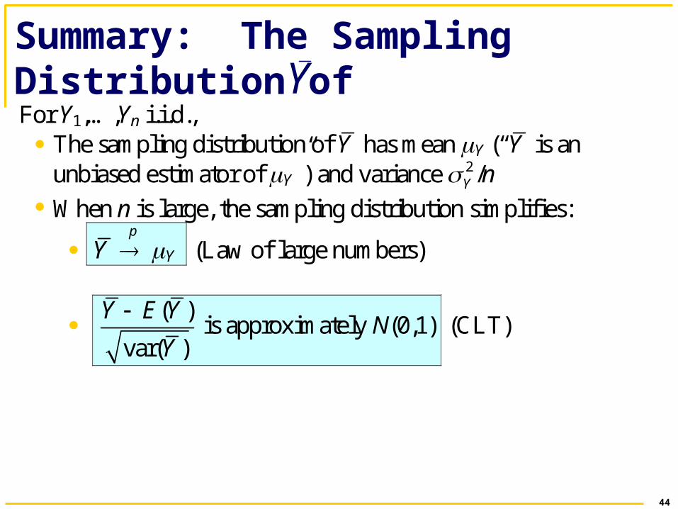
Summary: The Sampling Distribution of YFor Y1,…,Yn i.i.d., The sampling distribution of Y has mean Y (“Y is an
unbiased estimator of Y”) and variance 2Y /n
When n is large, the sampling distribution simplifies:
Y p
Y (Law of large numbers)
( )
var( )
Y E Y
Y
is approximately N(0,1) (CLT)
45
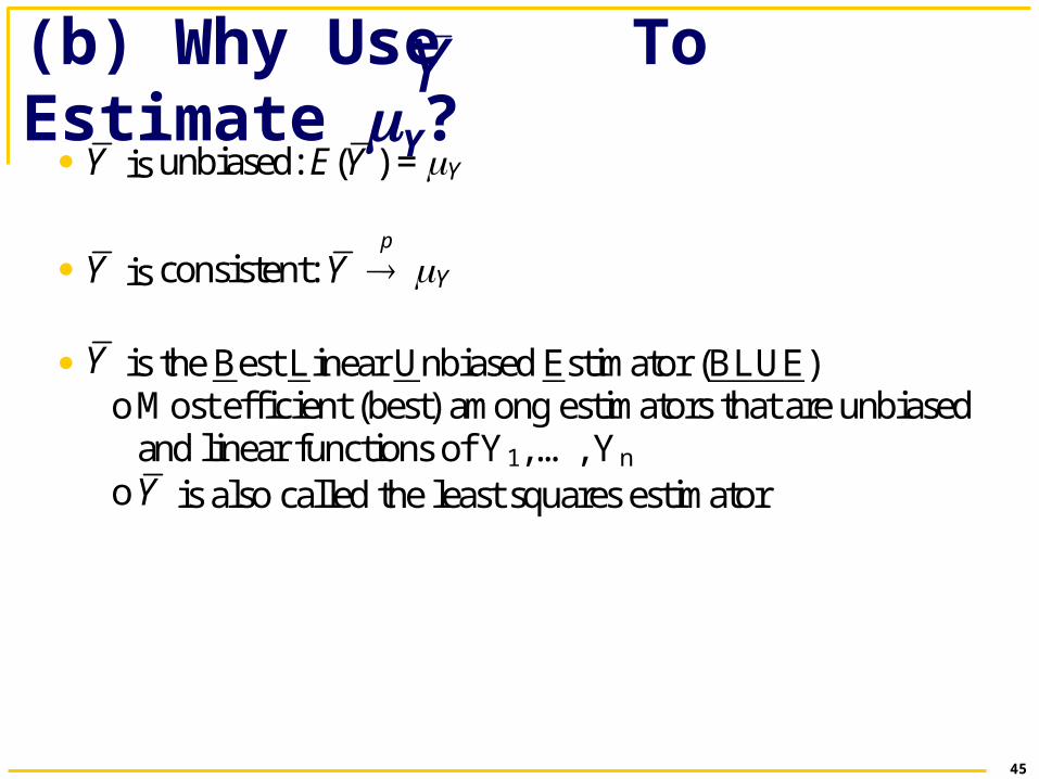
(b) Why Use To Estimate Y? Y Y is unbiased: E(Y ) = Y
Y is consistent: Y p
Y
Y is the Best Linear Unbiased Estimator (BLUE) o Most efficient (best) among estimators that are unbiased
and linear functions of Y1, …, Yn o Y is also called the least squares estimator
46
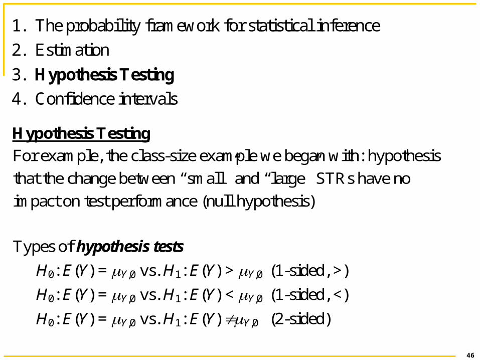
1. The probability framework for statistical inference
2. Estimation
3. Hypothesis Testing
4. Confidence intervals
Hypothesis Testing
For example, the class-size example we began with: hypothesis
that the change between “small” and “large” STRs have no
impact on test performance (null hypothesis)
Types of hypothesis tests
H0: E(Y) = Y,0 vs. H1: E(Y) > Y,0 (1-sided, >)
H0: E(Y) = Y,0 vs. H1: E(Y) < Y,0 (1-sided, <)
H0: E(Y) = Y,0 vs. H1: E(Y) Y,0 (2-sided)
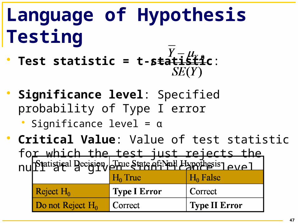
Test statistic = t-statistic:
Significance level: Specified probability of Type I error Significance level = α
Critical Value: Value of test statistic for which the test just rejects the null at a given significance level
Language of Hypothesis Testing
47
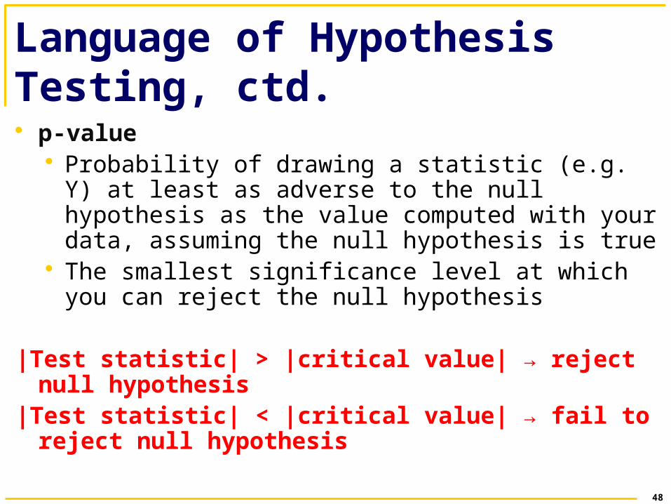
Language of Hypothesis Testing, ctd. p-value
Probability of drawing a statistic (e.g. Y) at least as adverse to the null hypothesis as the value computed with your data, assuming the null hypothesis is true
The smallest significance level at which you can reject the null hypothesis
|Test statistic| > |critical value| → reject null hypothesis|Test statistic| < |critical value| → fail to reject null
hypothesis
48
49
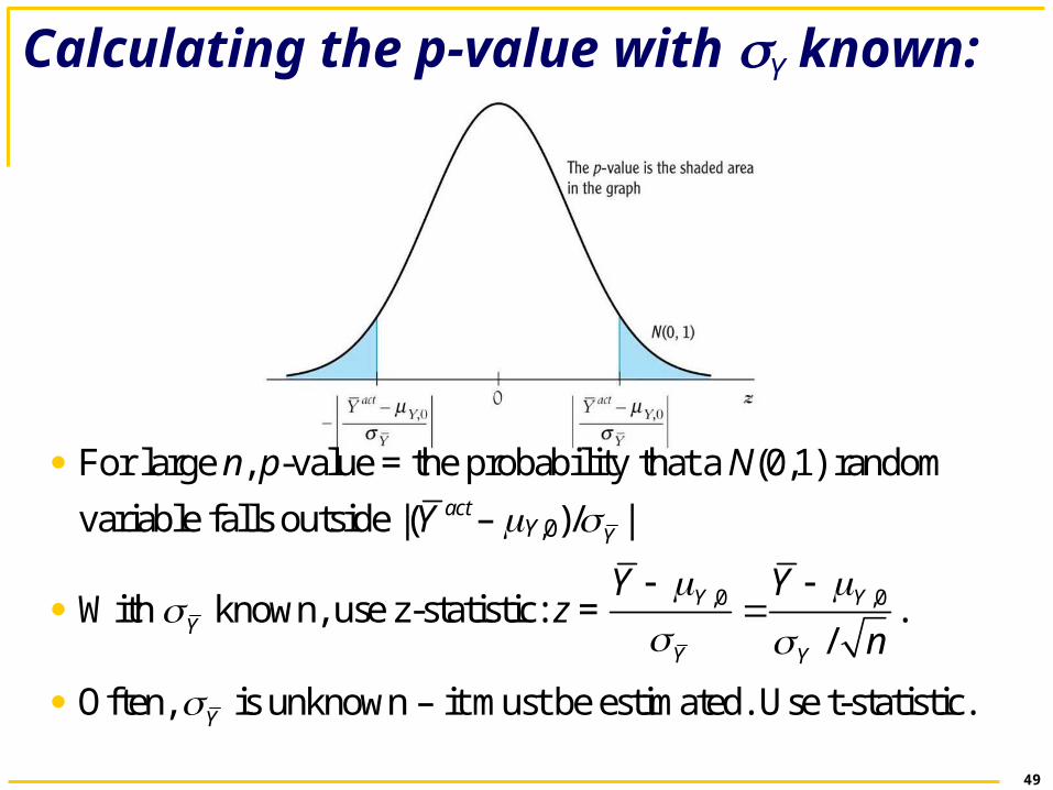
Calculating the p-value with Y known:
For large n, p-value = the probability that a N(0,1) random
variable falls outside |( actY – Y,0)/ Y |
With Y known, use z-statistic: z = ,0 ,0
/Y Y
Y Y
Y Y
n
.
Often, Y is unknown – it must be estimated. Use t-statistic.
50
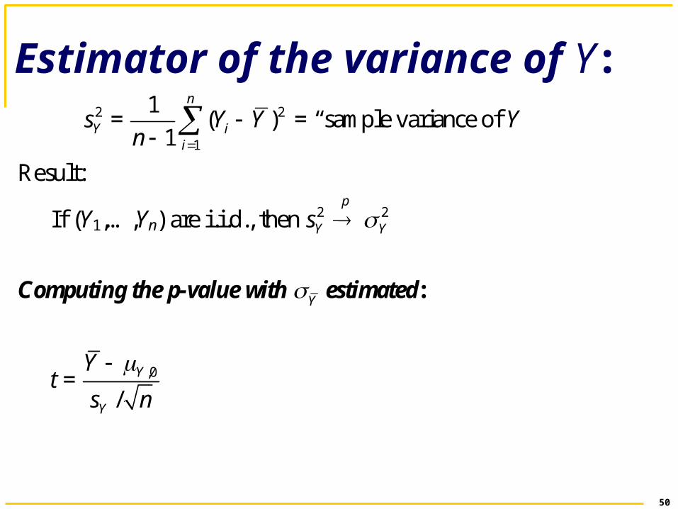
Estimator of the variance of Y: 2Ys = 2
1
1( )
1
n
ii
Y Yn
= “sample variance of Y”
Result:
If (Y1,…,Yn) are i.i.d., then 2Ys
p
2Y
Computing the p-value with Y estimated:
t = ,0
/Y
Y
Y
s n
51
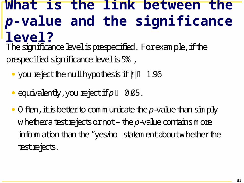
What is the link between the p-value and the significance level? The significance level is prespecified. For example, if the
prespecified significance level is 5%,
you reject the null hypothesis if |t| 1.96
equivalently, you reject if p 0.05.
Often, it is better to communicate the p-value than simply
whether a test rejects or not – the p-value contains more
information than the “yes/no” statement about whether the
test rejects.
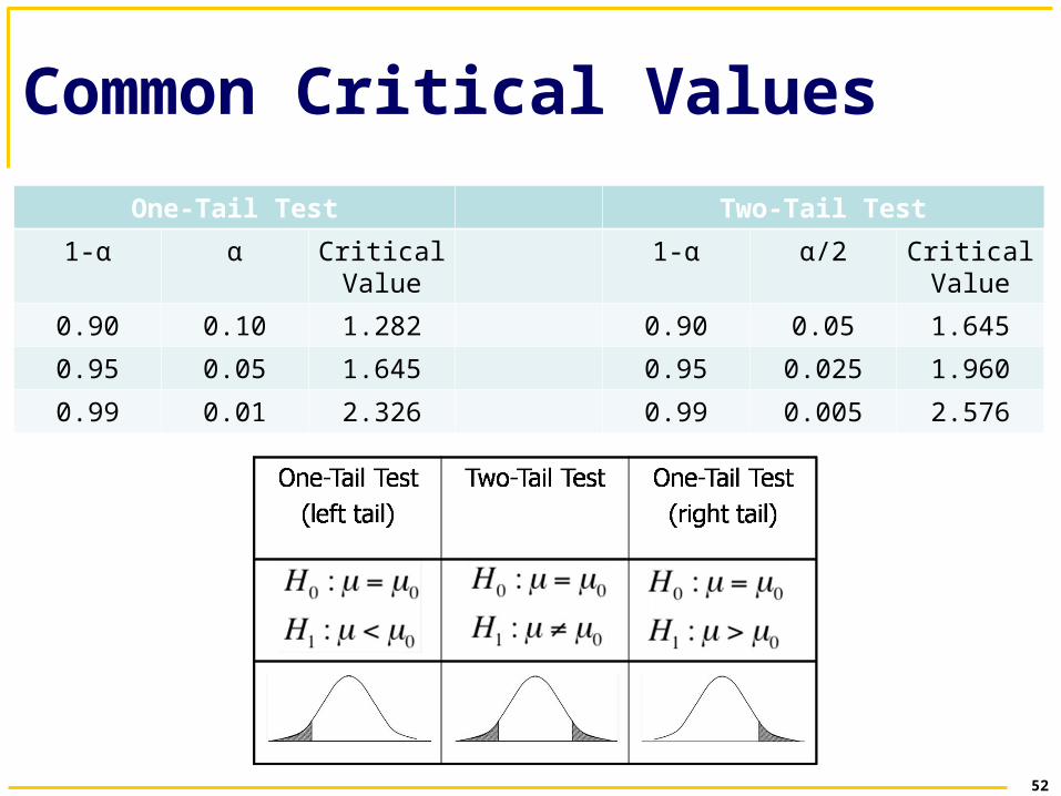
Common Critical Values
One-Tail Test Two-Tail Test
1-α α Critical Value
1-α α/2 Critical Value
0.90 0.10 1.282 0.90 0.05 1.645
0.95 0.05 1.645 0.95 0.025 1.960
0.99 0.01 2.326 0.99 0.005 2.576
52
53
1. The probability framework for statistical inference
2. Estimation
3. Testing
4. Confidence intervals
Confidence Intervals
A 95% confidence interval for Y is an interval that contains the
true value of Y in 95% of repeated samples.
Important point about discussing confidence intervals: What is random here? The values of Y1,…,Yn and thus any functions of them – including the confidence interval. The confidence interval will differ from one sample to the next. The population parameter, Y, is not random; we just don’t know it.


