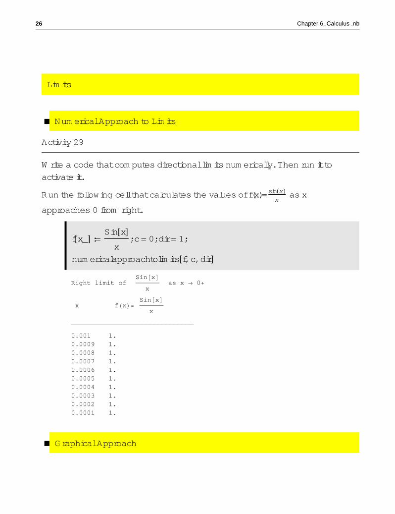
Chapter 6 : Calculus 06-01 Limits Activity 1 Run the following cell that gives the limit of sinHx L x as x fi 0. Limit@Sin@xD x, x fi 0D 1 Run the following cell that gives the limit of 1 x first as xfi0 - and then as xfi 0 + . N o t e : The limit is by default taken from above (right). Directional Limit : +1 means left,-1 means right. Limit@1 x, x -> 0, Direction -> 1D -¥ Limit@1 x, x -> 0, Direction -> - 1D ¥ Activity 2 Mathematica can't evaluate the limit of the greatest integer function as xfi
Transcript
Chapter 6 : Calculus
06-01 Limits
Activity 1
Run the following cell that gives the limit of sinHx Lx
as x ® 0.
Limit@Sin@xD � x, x ® 0D1
Run the following cell that gives the limit of 1x
first as x®0- and then as x®
0+.
Note: The limit is by default taken from above (right).
Directional Limit : +1 means left,-1 means right.
Limit@1 � x, x -> 0, Direction -> 1D-¥
Limit@1 � x, x -> 0, Direction -> -1D¥
Activity 2
Mathematica can't evaluate the limit of the greatest integer function as x®1-. Run the following cell.
Mathematica can't evaluate the limit of the greatest integer function as x®1-. Run the following cell.
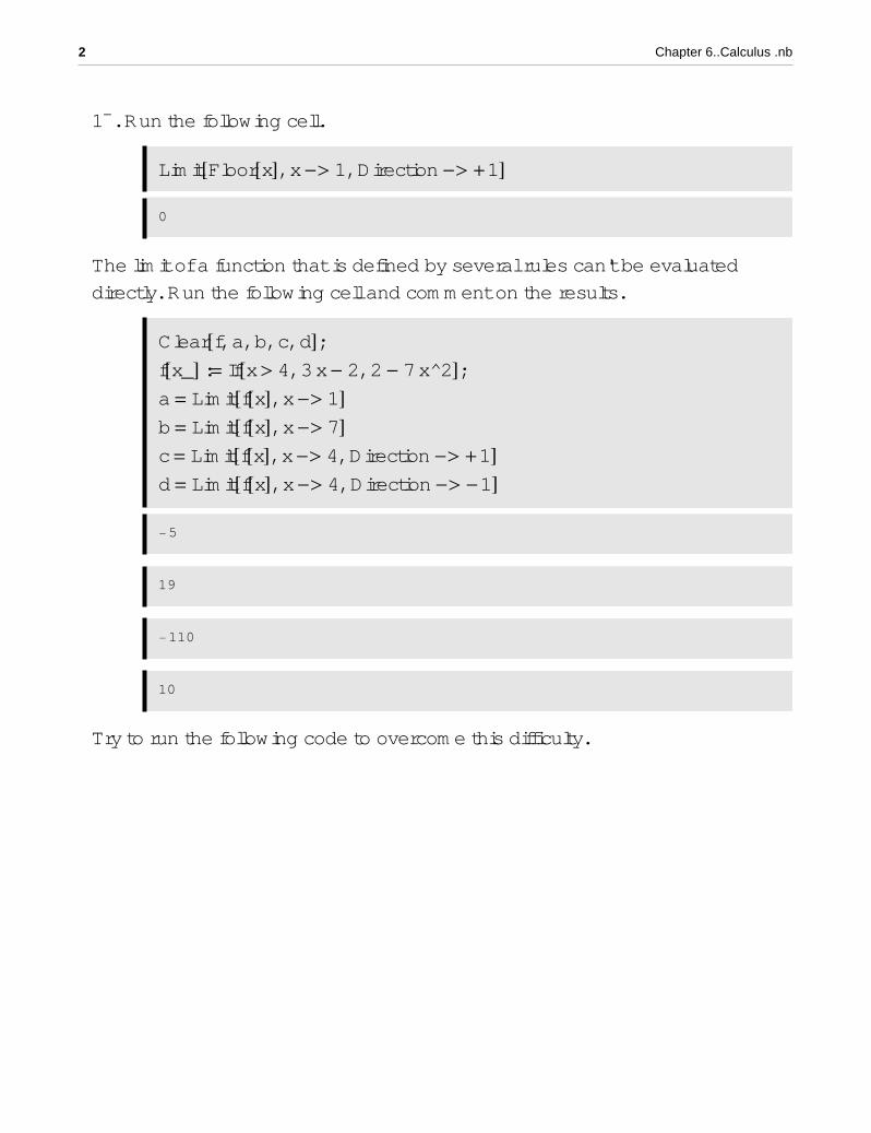
Limit@Floor@xD, x -> 1, Direction -> +1D0
The limit of a function that is defined by several rules can't be evaluated directly. Run the following cell and comment on the results.
Clear@f, a, b, c, dD;f@x_D := If@x > 4, 3 x - 2, 2 - 7 x^2D;a = Limit@f@xD, x -> 1Db = Limit@f@xD, x -> 7Dc = Limit@f@xD, x -> 4, Direction -> +1Dd = Limit@f@xD, x -> 4, Direction -> -1D-5
19
-110
10
Try to run the following code to overcome this difficulty.
2 Chapter 6..Calculus .nb
fup4@x_D := 3 x - 2;
fbelow4@x_D := 2 - 7 x^2;
a = Limit@fbelow4@xD, x -> 1Db = Limit@fup4@xD, x -> 7Dc = Limit@fup4@xD, x -> 4Dd = Limit@fbelow4@xD, x -> 4D-5
19
10
-110
06-02 Differentiation
à Mathematica Commands for Differentiation Operations.
Activity 3
Run the following cell that gives ¶¶x
x n .
D[x^n, x]
n x-1+n
Run the following cell that gives the first three derivatives of f Hx L = x n
Chapter 6..Calculus .nb 3
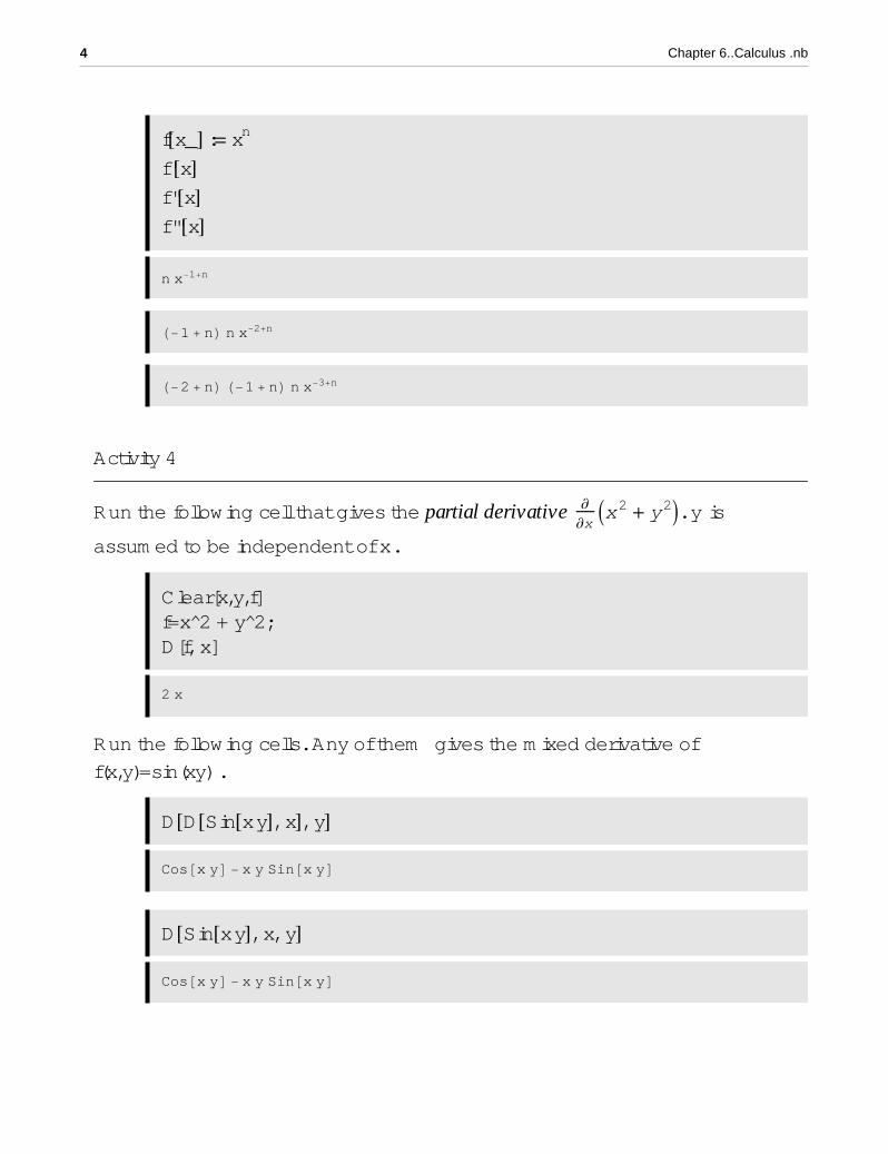
f@x_D := xn
f '@xDf ''@xDf '''@xDn x-1+n
H-1 + nL n x-2+n
H-2 + nL H-1 + nL n x-3+n
Activity 4
Run the following cell that gives the partial derivative ¶¶x
Ix 2 + y 2M. y is
assumed to be independent of x.
Clear[x,y,f]f=x^2 + y^2;D[f, x]
2 x
Run the following cells. Any of them gives the mixed derivative of f(x,y)=sin(xy) .
D@D@Sin@x yD, xD, yDCos@x yD - x y Sin@x yD
D@Sin@x yD, x, yDCos@x yD - x y Sin@x yD
4 Chapter 6..Calculus .nb
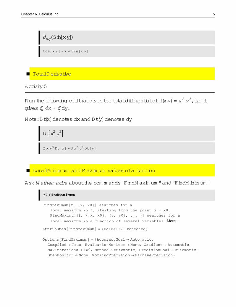
¶x,yHSin@x yDLCos@x yD - x y Sin@x yD
à Total Derivative
Activity 5
Run the following cell that gives the total differential of f(x,y) = x 2 y 3, i.e. it gives fx dx + fy dy.
Note: Dt[x] denotes dx and Dt[y] denotes dy
DtAx2 y3E2 x y3 Dt@xD + 3 x2 y2 Dt@yD
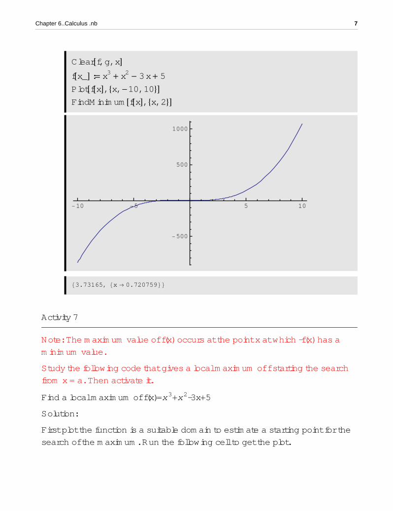
à Local Minimum and Maximum values of a function
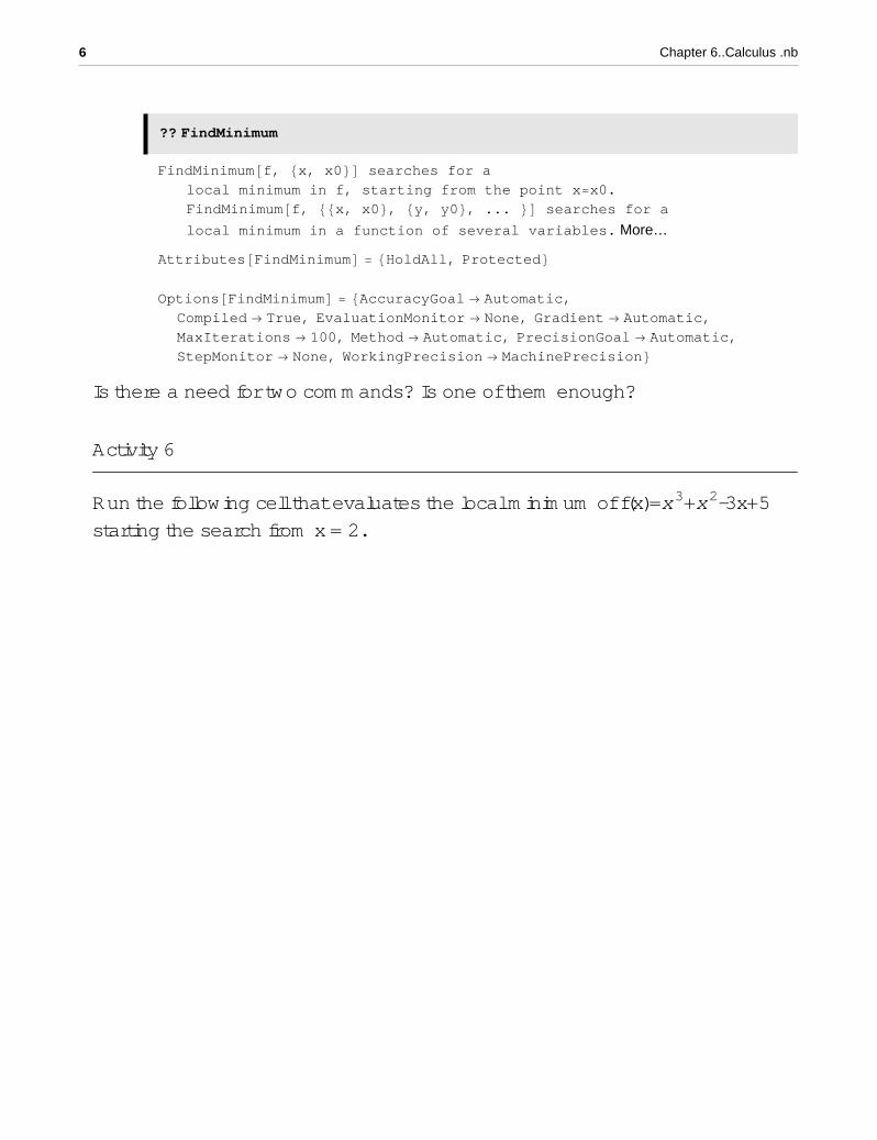
Ask Mathematica about the commands "FindMaximum" and "FindMinimum"
?? FindMaximum
FindMaximum@f, 8x, x0<D searches for a
local maximum in f, starting from the point x = x0.
FindMaximum@f, 88x, x0<, 8y, y0<, ... <D searches for a
local maximum in a function of several variables. More…
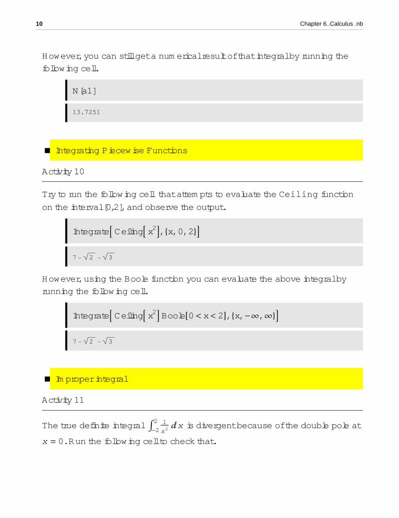
Run the following cell that tries to evaluate Ù0¥ sinHa x L
xâx .
Integrate[Sin[a x]/x, {x, 0, Infinity}]
-Π
2
Note that the If here gives the condition for the integral to be convergent.
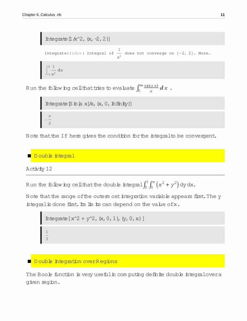
à Double integral
Activity 12
Run the following cell that the double integral Ù01Ù0
x Ix 2 + y 2M dy dx.
Note that the range of the outermost integration variable appears first. The y
integral is done first. Its limits can depend on the value of x.
Integrate[ x^2 + y^2, {x, 0, 1}, {y, 0, x} ]
1
3
à Double Integration over Regions
The Boole function is very useful in computing definite double integral over a given region.
Integrate[f[x] Boole[ ineq], {x, x1, x2}, {y, y1,y2} ] integrates the function f(x) over the region defined by all points satisfying the inequality inside the rectan-gle defined by values of x and y.
Note: You can use Integrate[f[x] Boole[ineq],{x,-¥,¥},{y,-¥,¥}] if you want Mathematica to select the inter region defined by the inequality.
Chapter 6..Calculus .nb 11
The Boole function is very useful in computing definite double integral over a given region.
Integrate[f[x] Boole[ ineq], {x, x1, x2}, {y, y1,y2} ] integrates the function f(x) over the region defined by all points satisfying the inequality inside the rectan-gle defined by values of x and y.
Note: You can use Integrate[f[x] Boole[ineq],{x,-¥,¥},{y,-¥,¥}] if you want Mathematica to select the inter region defined by the inequality.
Activity 13
Run the following cell that integrates x y + y 2 over the region R= {(x,y) : 0 £ x £ 1 and 0 £ y £ 1}.
IntegrateA x y + y2, 8x, 0, 1<, 8y, 0, 1< E7
12
Run the following cells . Comment on the obtained results. Write the inte-grals that have been evaluated..
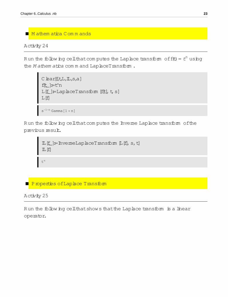
à Laplace Transform of nth derivative of a function
Activity 26
Laplace transforms have the property that they turn integration and differentia-tion into essentially algebraic operations. Run the following cell and com-ment on the output
extrempoints1@f, ΕD1L The function is fHxL = H-5 + xL H-1 + xL H2 + xL2L Its first derivative is f'HxL =H-5 + xL H-1 + xL + H-5 + xL H2 + xL + H-1 + xL H2 + xL3L The set of values of x such that f has critical points is
:13
J4 - 37 N, 1
3J4 + 37 N>
5L Classification of critical points based on second derivative test :
For point number 1 :
:13
J4 - 37 N, -5 +1
3J4 - 37 N -1 +
1
3J4 - 37 N 2 +
1
3J4 - 37 N >
is a maximum point
For point number 2 :
:13
J4 + 37 N, -5 +1
3J4 + 37 N -1 +
1
3J4 + 37 N 2 +
1
3J4 + 37 N >
is a minimum point
à Second Derivative Test for Local Extreme Points
Activity 36
Run the following cell.
Comment on the output.
Write a code that gives the same output.
Chapter 6..Calculus .nb 43
Clear@f, xDf@x_D := Hx - 1L Hx + 2L Hx - 5L;extrempoints2@fD1L The function is fHxL = H-5 + xL H-1 + xL H2 + xL2L Its first derivative is f'HxL =H-5 + xL H-1 + xL + H-5 + xL H2 + xL + H-1 + xL H2 + xL3L The set of values of x such that f has critical points is
:13
J4 - 37 N, 1
3J4 + 37 N>
4L The second derivative of f is f''HxL = -8 + 6 x
5L Classification of critical points based on second derivative test :