Challenges associated with studying nonlinear distortion of acoustic waveforms emitted by high-speed jets Woutijn J. BAARS 1 ; Charles E. TINNEY 2 ; Mark F. HAMILTON 3 1 Department of Mechanical Engineering, The University of Melbourne, Melbourne, VIC 3010, Australia 2 Center for Aeromechanics Research, The University of Texas at Austin, Austin, TX 78712, U.S.A. 3 Applied Research Laboratories, The University of Texas at Austin, Austin, TX 78713, U.S.A. ABSTRACT Discrepancies between linear predictions and direct measurements of the far-field sound produced by high- speed jet flows are typically ascribed to nonlinear distortion. Here we employ an effective Gol’dberg number to investigate the likelihood of nonlinear distortion in the noise fields of supersonic jets. This simplified ap- proach relies on an isolated view of a ray tube along the Mach wave angle. It is known that the acoustic pressure obeys by cylindrical spreading in close vicinity to the jet before advancing to a spherical decay in the far-field. Therefore, a ‘piecewise-spreading regime’ model is employed in order to compute effective Gol’dberg numbers for these jet flows. Our first-principal approach suggests that cumulative nonlinear distor- tion can only be present within 20 jet exit diameters along the Mach wave angle when laboratory-scale jets are being considered. Effective Gol’dberg numbers for full-scale jet noise scenarios reveal that a high-degree of cumulative distortion can likewise be present in the spherical decay regime. Hence, full-scale jet noise fields are more affected by cumulative distortion. Keywords: Jet Noise, Nonlinear Effects I-INCE Classification of Subjects Number(s): 21.6.1, 21.6.7/8 1. INTRODUCTION Active noise suppression systems for high-speed jets will rely on real-time noise estimation procedures, and therefore, their control effectiveness depends on the accuracy of the underlying physical models. Despite over a half century of research with compelling progress, a full understanding has yet to be gleaned on how pronounced such nonlinear distortion effects are in the acoustic waveforms emitted by high-speed jets. A comprehensive review of the literature pertaining to this topic is beyond the scope of this paper. Albeit significant contributions include the work of Ffowcs Williams et al. (1), Pestorius & Blackstock (2), Crighton & Bashforth (3), Morfey & Howell (4), Petitjean et al. (5), Saxena et al. (6), Gee et al. (7) and Baars et al. (8) and the references therein. It is common practice to categorize the noise features of supersonic jets according to their sound gen- erating mechanism. This includes turbulent mixing noise, broadband shock-associated noise, screech and transonic resonance (9). Shock-free supersonic jets solely possess mixing noise induced by both fine-scale and large-scale turbulence within the jet’s shear layer (10). When the convective speed of the turbulent large scales, U c , becomes higher than the ambient sound speed a ∞ , a distinct region of high-intensity sound is produced that is concentrated in the post-potential core of the jet. The acoustic waves produced by these large scales radiate along the Mach wave angle φ = cos −1 (a ∞ /U c ) and become more pronounced with increasing convective Mach number M c = U c /a ∞ . Figure 1 illustrates the acoustic field of an unheated and shock-free Mach 3 jet, as studied by Baars & Tinney (11), with a Mach wave angle of φ = 45 ◦ . The highest source intensity along the jet axis was identified to be at x ≈ 20D j , where x is the coordinate along the jet centerline and D j is the jet exit diameter; r is the radial coordinate. The sound intensity is highest along the Mach wave angle (12, 13, 14), and thus, nonlinear distortion would be most pronounced there due to its high dependence on the sound intensity. For this reason we confine ourselves to an artificial ray tube drawn in Figure 1. Cumulative nonlinear waveform distortion is commonly assumed to be a physical mechanism present in the sound field of supersonic jets. Discrepancies between predictions of the far-field sound (e.g. mapping near field spectra or waveforms) and direct measurements are often ascribed to nonlinear distortion when the far 1 [email protected]Inter-noise 2014 Page 1 of 10
Transcript
Challenges associated with studying nonlinear distortion of acousticwaveforms emitted by high-speed jets
Woutijn J. BAARS1; Charles E. TINNEY2; Mark F. HAMILTON3
1 Department of Mechanical Engineering, The University of Melbourne, Melbourne, VIC 3010, Australia2 Center for Aeromechanics Research, The University of Texasat Austin, Austin, TX 78712, U.S.A.
3 Applied Research Laboratories, The University of Texas at Austin, Austin, TX 78713, U.S.A.
ABSTRACTDiscrepancies between linear predictions and direct measurements of the far-field sound produced by high-speed jet flows are typically ascribed to nonlinear distortion. Here we employ an effective Gol’dberg numberto investigate the likelihood of nonlinear distortion in the noise fields of supersonic jets. This simplified ap-proach relies on an isolated view of a ray tube along the Mach wave angle. It is known that the acousticpressure obeys by cylindrical spreading in close vicinity to the jet before advancing to a spherical decayin the far-field. Therefore, a ‘piecewise-spreading regime’ model is employed in order to compute effectiveGol’dberg numbers for these jet flows. Our first-principal approach suggests that cumulative nonlinear distor-tion can only be present within 20 jet exit diameters along the Mach wave angle when laboratory-scale jetsare being considered. Effective Gol’dberg numbers for full-scale jet noise scenarios reveal that a high-degreeof cumulative distortion can likewise be present in the spherical decay regime. Hence, full-scale jet noisefields are more affected by cumulative distortion.
1. INTRODUCTIONActive noise suppression systems for high-speed jets will rely on real-time noise estimation procedures,
and therefore, their control effectiveness depends on the accuracy of the underlying physical models. Despiteover a half century of research with compelling progress, a full understanding has yet to be gleaned onhow pronounced such nonlinear distortion effects are in the acoustic waveforms emitted by high-speed jets.A comprehensive review of the literature pertaining to thistopic is beyond the scope of this paper. Albeitsignificant contributions include the work of Ffowcs Williamset al.(1), Pestorius & Blackstock (2), Crighton& Bashforth (3), Morfey & Howell (4), Petitjeanet al.(5), Saxenaet al.(6), Geeet al.(7) and Baarset al.(8)and the references therein.
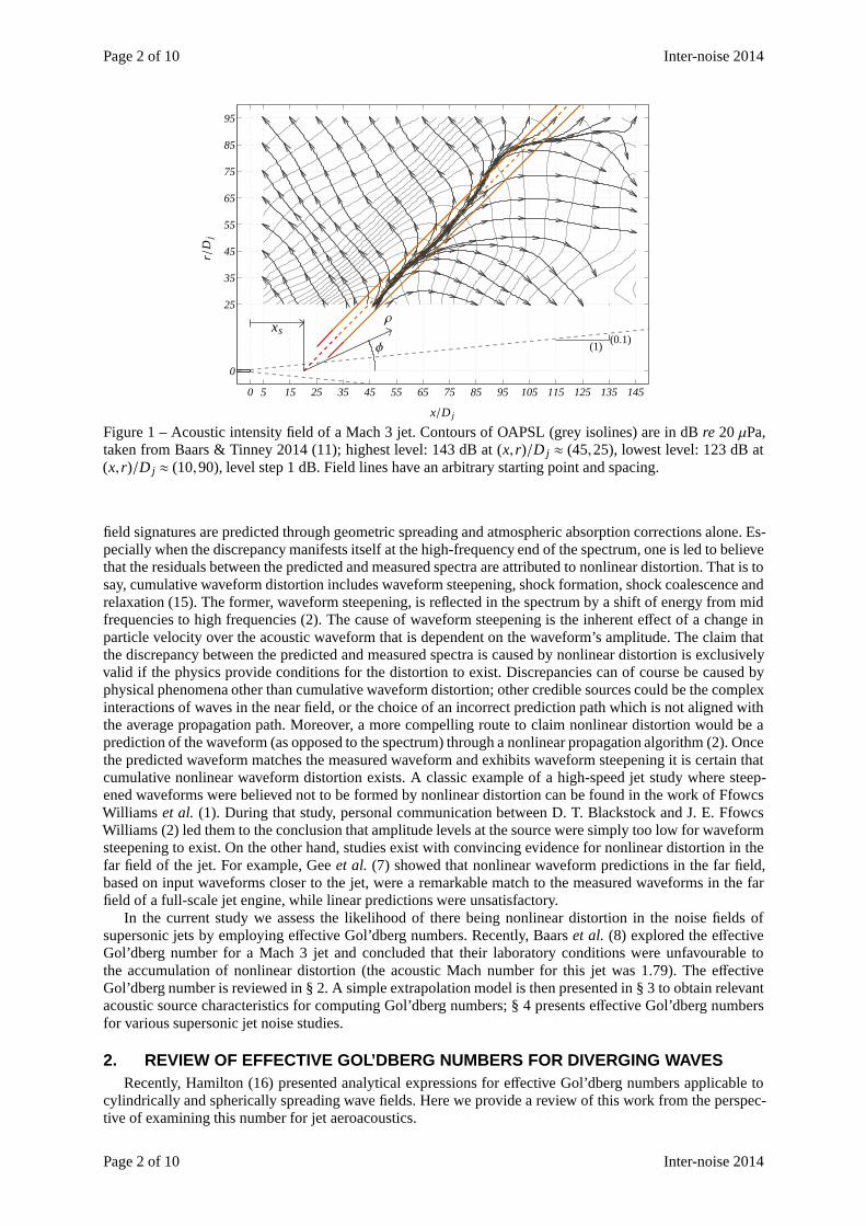
It is common practice to categorize the noise features of supersonic jets according to their sound gen-erating mechanism. This includes turbulent mixing noise, broadband shock-associated noise, screech andtransonic resonance (9). Shock-free supersonic jets solely possess mixing noise induced by both fine-scaleand large-scale turbulence within the jet’s shear layer (10). When the convective speed of the turbulent largescales,Uc, becomes higher than the ambient sound speeda∞, a distinct region of high-intensity sound isproduced that is concentrated in the post-potential core ofthe jet. The acoustic waves produced by these largescales radiate along the Mach wave angleφ = cos−1 (a∞/Uc) and become more pronounced with increasingconvective Mach numberMc = Uc/a∞. Figure 1 illustrates the acoustic field of an unheated and shock-freeMach 3 jet, as studied by Baars & Tinney (11), with a Mach wave angle of φ = 45◦. The highest sourceintensity along the jet axis was identified to be atx≈ 20D j, wherex is the coordinate along the jet centerlineandD j is the jet exit diameter;r is the radial coordinate. The sound intensity is highest along the Mach waveangle (12, 13, 14), and thus, nonlinear distortion would be most pronounced there due to its high dependenceon the sound intensity. For this reason we confine ourselves to an artificial ray tube drawn in Figure 1.
Cumulative nonlinear waveform distortion is commonly assumed to be a physical mechanism present inthe sound field of supersonic jets. Discrepancies between predictions of the far-field sound (e.g.mapping nearfield spectra or waveforms) and direct measurements are often ascribed to nonlinear distortion when the far
Figure 1 – Acoustic intensity field of a Mach 3 jet. Contours ofOAPSL (grey isolines) are in dBre 20 µPa,taken from Baars & Tinney 2014 (11); highest level: 143 dB at (x, r)/D j ≈ (45,25), lowest level: 123 dB at(x, r)/D j ≈ (10,90), level step 1 dB. Field lines have an arbitrary starting point and spacing.
field signatures are predicted through geometric spreadingand atmospheric absorption corrections alone. Es-pecially when the discrepancy manifests itself at the high-frequency end of the spectrum, one is led to believethat the residuals between the predicted and measured spectra are attributed to nonlinear distortion. That is tosay, cumulative waveform distortion includes waveform steepening, shock formation, shock coalescence andrelaxation (15). The former, waveform steepening, is reflected in the spectrum by a shift of energy from midfrequencies to high frequencies (2). The cause of waveform steepening is the inherent effect of a change inparticle velocity over the acoustic waveform that is dependent on the waveform’s amplitude. The claim thatthe discrepancy between the predicted and measured spectrais caused by nonlinear distortion is exclusivelyvalid if the physics provide conditions for the distortion to exist. Discrepancies can of course be caused byphysical phenomena other than cumulative waveform distortion; other credible sources could be the complexinteractions of waves in the near field, or the choice of an incorrect prediction path which is not aligned withthe average propagation path. Moreover, a more compelling route to claim nonlinear distortion would be aprediction of the waveform (as opposed to the spectrum) through a nonlinear propagation algorithm (2). Oncethe predicted waveform matches the measured waveform and exhibits waveform steepening it is certain thatcumulative nonlinear waveform distortion exists. A classic example of a high-speed jet study where steep-ened waveforms were believed not to be formed by nonlinear distortion can be found in the work of FfowcsWilliams et al. (1). During that study, personal communication between D. T. Blackstock and J. E. FfowcsWilliams (2) led them to the conclusion that amplitude levels at the source were simply too low for waveformsteepening to exist. On the other hand, studies exist with convincing evidence for nonlinear distortion in thefar field of the jet. For example, Geeet al. (7) showed that nonlinear waveform predictions in the far field,based on input waveforms closer to the jet, were a remarkablematch to the measured waveforms in the farfield of a full-scale jet engine, while linear predictions were unsatisfactory.
In the current study we assess the likelihood of there being nonlinear distortion in the noise fields ofsupersonic jets by employing effective Gol’dberg numbers. Recently, Baarset al. (8) explored the effectiveGol’dberg number for a Mach 3 jet and concluded that their laboratory conditions were unfavourable tothe accumulation of nonlinear distortion (the acoustic Mach number for this jet was 1.79). The effectiveGol’dberg number is reviewed in § 2. A simple extrapolation model is then presented in § 3 to obtain relevantacoustic source characteristics for computing Gol’dberg numbers; § 4 presents effective Gol’dberg numbersfor various supersonic jet noise studies.
2. REVIEW OF EFFECTIVE GOL’DBERG NUMBERS FOR DIVERGING WAVESRecently, Hamilton (16) presented analytical expressionsfor effective Gol’dberg numbers applicable to
cylindrically and spherically spreading wave fields. Here we provide a review of this work from the perspec-tive of examining this number for jet aeroacoustics.
Page 2 of 10 Inter-noise 2014
Inter-noise 2014 Page 3 of 10
To determine the likelihood of cumulative nonlinear distortion, one must consider the relative strengthof two competing effects: nonlinear distortion and energy absorption, the strengths of which are commonlyexpressed in terms of their individual length scales. We begin with expressions for planar wave fields, as theexpressions for cylindrical and spherical spreading wavesare based on this. The first length scale, the acousticabsorption length, is simply the reciprocal of the absorption coefficient,la = 1/α, and reflects the strength ofenergy absorption. The second length scale, which is associated with nonlinear distortion, is the plane waveshock formation distance, and is defined as
x=ρ∞a3
∞
β (2π f0) prms, (1)
whereβ= (γ+1)/2= 1.2 is the coefficient of nonlinearity for air,prms is the standard deviation of the acousticpressure andf0 is the characteristic frequency associated with the source.1 The Gol’dberg number for planarwaves is then defined as the ratio of the aforementioned length scales,
Γ =lax, (2)
which appears naturally as the coefficient in front of the nonlinear term in the nondimensional form of thegeneralized Burgers equation (Hamilton & Blackstock (15),p. 312). ForΓ . 1, attenuation dominates andthe formation of shocks is suppressed. Conversely, whenΓ≫ 1, cumulative nonlinear distortion is likely tooccur. For jet noise applications, the representative acoustic signal at the source is relatively broadband; ahump resides which offers some relief when selecting a characteristic frequency for computing the Gol’dbergnumber. Finally, the frequency dependent absorption coefficientα ( f ) is taken atf = f0 for a thermoviscousfluid with relaxation; see App. B of Blackstock (17).
Turning our attention now to diverging waves,e.g.cylindrical or spherical spreading fields, a third lengthscale is considered: the source radiusr0, which is often expressed relative to the plane wave shock formationdistance according toσ0 = r0/x. While the evolution of a plane wave is determined completely by the singleparameterΓ, two dimensionless parameters—length scale ratiosΓ andσ0—determine the likelihood of non-linear distortion in diverging wave fields. As reported by Hamilton (16), theeffectiveGol’dberg numbers forcylindrical waves and spherical waves are given by Eqs. (3a)and (3b), respectively.
Λc =Γ
1+ ζsh/ (2σ0), (3a)
Λs = Γexp(−ζsh/σ0) . (3b)
Here, the constantζsh is taken asζsh = π/2 and is motivated by the fact thatΛ can now be interpreted ina similar manner asΓ from the perspective of the likelihood of cumulative nonlinear distortion to producesawtooth waveforms. In this context, shock formation is guaranteed forΛ≫ 1, whereas nonlinear effects aresuppressed and negligible forΛ . 1. It is important to mention that an underlying assumption for Eq. (3)is that the conditionk0r0 ≫ 1 should be satisfied, wherek0 = 2π f0/a∞. Finally, an independent nonlinearlength scale to compute the shock formation distance for spherically diverging waves is used and is definedas:r = r0exp(σ0).
It is apparent from Eqs. (2), (3a) and (3b) that the Gol’dbergnumber is dependent on the source centerfrequencyf0, amplitudeprms and radiusr0. As we will consider a collection of supersonic jet noise studies inthis analysis, it is inevitable thatf0, prms andr0 will change such that the necessary conditions for nonlineardistortion are altered. For example, when a full-scale jet engine is geometrically scaled to a sub-scale size, asis commonly encountered in laboratory-environments,f0 increases andr0 decreases. The simplest scenariothen is one that comprises aerodynamic similarity, such that the exit Mach numberM j , exit temperatureratio T j/T∞ and hence the exit velocityU j , remain constant. In doing so, the Strouhal number remainsconstant (StD j = f0D j/U j), thereby allowing the center frequency to scale accordingly. Henceforth, frequencyscales asf0 ∝ 1/D j while source size scales asr0 ∝ D j . Furthermore, assuming that the acoustic sourceintensity is proportional to the exit velocity to a certain powerb, then the source amplitudeprms∝Ub/2
j shouldremain constant for an aerodynamically scaled jet. Unfortunately, under these assumptions, the effectiveGol’dberg numbers for the full-scale and laboratory-scalestudy would not match. Thus for theacousticspartof study, the effective Gol’dberg number should ideally be of the same order of magnitude, or at least in the
1Throughout this paper, Gol’dberg numbers are computed for standard temperature and pressure (STP) conditions ofp∞ = 101,325 Pa andT∞ =293.15 K; hence the ambient density and sound speed areρ∞ = p∞/R/T∞ anda∞ =
√γRT∞, respectively.
Inter-noise 2014 Page 3 of 10
Page 4 of 10 Inter-noise 2014
same regime for scaled studies (e.g.Λ . 1 orΛ≫ 1)2. It is important to emphasize the common practice ofconsidering only similarity parameters such asM j , T j/T∞ and Reynolds number ReD j when replicating afull-scale jet engine by way of laboratory-scale experiments. Thus, the effective Gol’dberg number is oftenoverlooked as the parametersM j, T j/T∞ and ReD j only govern the similarity of theaerodynamics. As wasrecognized previously (16), the Gol’dberg number can be interpreted as an acoustic Reynolds number andis equally imperative when using laboratory scale noise measurements to predict the acoustic waveformsproduced by full-scale engines.
3. SUPERSONIC JET NOISE SOURCE CHARACTERISTICSHere we present a simple extrapolation method in § 3.1 to obtain the acoustic source parameters necessary
for computing effective Gol’dberg numbers using a ‘piecewise-spreading regime’ model; thereafter we applythis model to various high-speed jet noise studies from the literature (§ 3.2).
3.1 Extrapolation Model to Obtain Source ParametersDefining the correct set of acoustic source parameters that represent the distribution of sources throughout
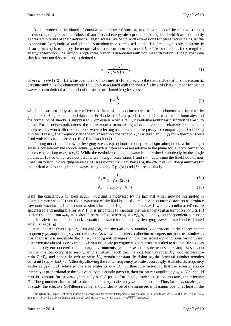
the jet’s shear layer is challenging. It became evident thatwe require three source parameters for comput-ing effective Gol’dberg numbers: the center frequency, the standard deviation of the acoustic pressure and thesource radius. Furthermore, we confine ourselves to an artificial ray tube originating from the location of high-est source intensity on the jet axis, that is oriented along the Mach wave angle (see Figure 1). We do this toencapsulate the correct propagation path of most intense sound generated by the convection of large-scale tur-bulence (18). To investigate the acoustic pressure decay along this ray tube we employ a wave packet model;its theoretical framework is discussed by Morris (18), Papamoschou (19) and others. Following the outlineprovided in App. A of Baars (20) and in Fiévetet al. (21), the pressure field resulting from the evolution ofthe jet’s large-scale instabilities are presented in Figure 1 and are necessary to estimate the acoustic pressuredecay along the ray tube (coordinateρ) as presented in Figure 2a. Laboratory measurements using1/4 in. (11)and1/8 in. microphones (21) are superimposed this wave packet model (corrected for atmospheric absorptionbased on STP and a relative humidity of 70%). It is important to mention that a wave packet length scale,
2 3 4 5 6 7 8 910 20 30 40 50 60 80 100 140
0.1
0.2
0.3
0.40.50.6
0.81
2
wave packet model
ρ/D j
p rm
s(k
Pa)
Baarset al. (11) 1/4 in. gridBaarset al. (11) 1/4 in. lineFiévetet al. (21) 1/8 in.
∝ 1√ρ
∝ 1ρ
∝ 1ρ
r0D j= s0
r1D j= s1
x, jet axis
measurement:
pmrms, fm atρ = rm
φ
x= xs
r0
r1
prms(r1) = pmrms
rmr1
prms(r0) =
pmrms
rmr1
√
r1r0
ρ
(a) (b)
+ abs. corr.
+ abs. corr.
Figure 2 – (a) Pressure decay of the wave packet model fitted tothe experimental measurements of Baars &Tinney (11) and Fiévetet al. (21). (b) Concept of simple extrapolation towards the source.
relative to the scale of the jet, had to be selected, which wasdenoted as parameterA1 = L/D j (20). Here,L isthe length scale of a wave packet comprising a harmonic wave with a Gaussian envelopeA(x) ∝ exp
(
−x2/L2)
.By fitting the wave packet model decay trend to the experimental data, the value of the wave packet parame-ter is found to beA1 = 8.75. Thus, in close vicinity to the wave packet source, the acoustic pressure decay isshown to abide by cylindrical spreading (prms∝ 1/
√ρ), while the pressure spreads spherically in the far field
(prms∝ 1/ρ). To complete this ‘piecewise-spreading regime’ model we require a source radiusr0 and a ranger1 at which the decay transitions from cylindrical to spherical. Baarset al. (8) assumes that the source size isproportional to the jet diameter,r0 = s0D j , with a scale ofs0 = 2.5; this was driven by an estimated shear layergrowth of 0.1x and a source location atx ≈ 20D j. The scale for locationr1 can be retrieved from Figure 2a
2The reader is referred to Baarset al. (8) for a more detailed discussion of the arguments supporting this scaling analysis.
Page 4 of 10 Inter-noise 2014
Inter-noise 2014 Page 5 of 10
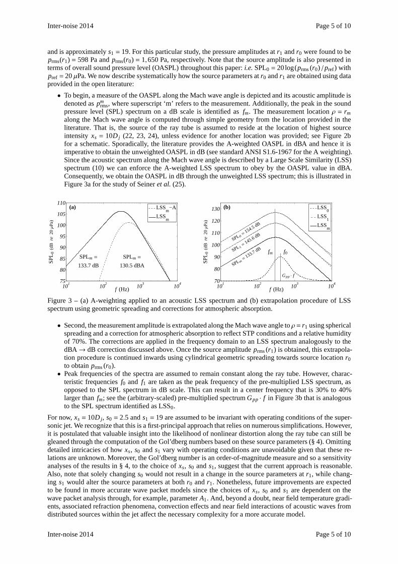
and is approximatelys1 = 19. For this particular study, the pressure amplitudes atr1 andr0 were found to beprms(r1) = 598 Pa andprms(r0) = 1,650 Pa, respectively. Note that the source amplitude is alsopresented interms of overall sound pressure level (OASPL) throughout this paper:i.e.SPL0 = 20 log(prms(r0)/pref) withpref = 20µPa. We now describe systematically how the source parameters atr0 andr1 are obtained using dataprovided in the open literature:
• To begin, a measure of the OASPL along the Mach wave angle is depicted and its acoustic amplitude isdenoted aspm
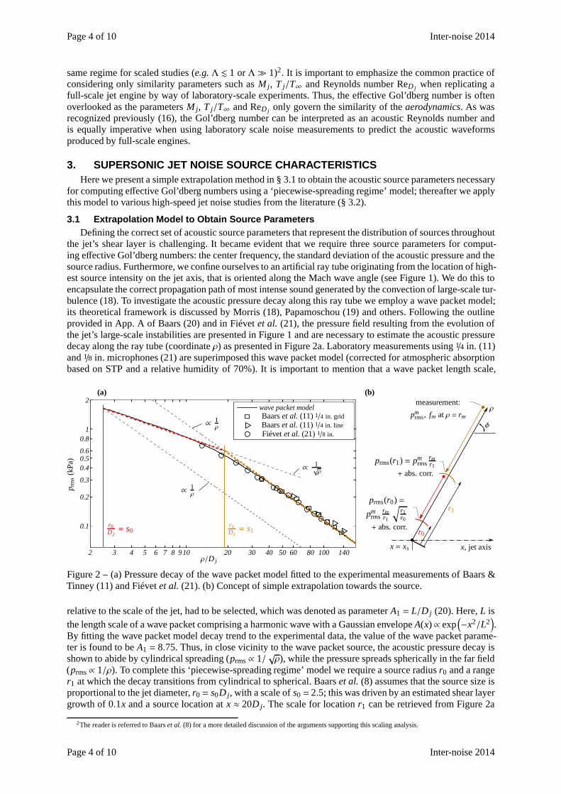
rms, where superscript ‘m’ refers to the measurement. Additionally, the peak in the soundpressure level (SPL) spectrum on a dB scale is identified asfm. The measurement locationρ = rmalong the Mach wave angle is computed through simple geometry from the location provided in theliterature. That is, the source of the ray tube is assumed to reside at the location of highest sourceintensity xs = 10D j (22, 23, 24), unless evidence for another location was provided; see Figure 2bfor a schematic. Sporadically, the literature provides theA-weighted OASPL in dBA and hence it isimperative to obtain the unweighted OASPL in dB (see standard ANSI S1.6-1967 for the A weighting).Since the acoustic spectrum along the Mach wave angle is described by a Large Scale Similarity (LSS)spectrum (10) we can enforce the A-weighted LSS spectrum to obey by the OASPL value in dBA.Consequently, we obtain the OASPL in dB through the unweighted LSS spectrum; this is illustrated inFigure 3a for the study of Seineret al. (25).
101
102
103
10475
80
85
90
95
100
105
110
LSSm
−A
LSSm
f (Hz)
SP
L 0(d
Bre
20µP
a)
SPLm =
130.5 dBA
SPLm =
133.7 dB
(a)
101
102
103
10470
80
90
100
110
120
130
LSS0
LSS1
LSSm
f (Hz)
SP
L 0(d
Bre
20µP
a)
SPLm=
133.7dBSPL1
=145.6
dBSPL0
=154.5
dB
fm f0
Gpp · f
(b)
Figure 3 – (a) A-weighting applied to an acoustic LSS spectrum and (b) extrapolation procedure of LSSspectrum using geometric spreading and corrections for atmospheric absorption.
• Second, the measurement amplitude is extrapolated along the Mach wave angle toρ= r1 using sphericalspreading and a correction for atmospheric absorption to reflect STP conditions and a relative humidityof 70%. The corrections are applied in the frequency domain to an LSS spectrum analogously to thedBA→ dB correction discussed above. Once the source amplitudeprms(r1) is obtained, this extrapola-tion procedure is continued inwards using cylindrical geometric spreading towards source locationr0to obtainprms(r0).• Peak frequencies of the spectra are assumed to remain constant along the ray tube. However, charac-
teristic frequenciesf0 and f1 are taken as the peak frequency of the pre-multiplied LSS spectrum, asopposed to the SPL spectrum in dB scale. This can result in a center frequency that is 30% to 40%larger thanfm; see the (arbitrary-scaled) pre-multiplied spectrumGpp · f in Figure 3b that is analogousto the SPL spectrum identified as LSS0.
For now,xs = 10D j, s0 = 2.5 ands1 = 19 are assumed to be invariant with operating conditions of the super-sonic jet. We recognize that this is a first-principal approach that relies on numerous simplifications. However,it is postulated that valuable insight into the likelihood of nonlinear distortion along the ray tube can still begleaned through the computation of the Gol’dberg numbers based on these source parameters (§ 4). Omittingdetailed intricacies of howxs, s0 ands1 vary with operating conditions are unavoidable given that these re-lations are unknown. Moreover, the Gol’dberg number is an order-of-magnitude measure and so a sensitivityanalyses of the results in § 4, to the choice ofxs, s0 ands1, suggest that the current approach is reasonable.Also, note that solely changings0 would not result in a change in the source parameters atr1, while chang-ing s1 would alter the source parameters at bothr0 andr1. Nonetheless, future improvements are expectedto be found in more accurate wave packet models since the choices ofxs, s0 and s1 are dependent on thewave packet analysis through, for example, parameterA1. And, beyond a doubt, near field temperature gradi-ents, associated refraction phenomena, convection effects and near field interactions of acoustic waves fromdistributed sources within the jet affect the necessary complexity for a more accurate model.
Inter-noise 2014 Page 5 of 10
Page 6 of 10 Inter-noise 2014
3.2 Source Characteristics of Supersonic Jet Noise StudiesThe model for obtaining source parameters atr0 andr1 is applied to various studies from the literature.
Table 1 lists the selected high-speed jet studies with theirmost significant operating parameters, sorted ac-cording to scale. Source parameters atr0 andr1 are listed, as well as an indication as to whether the study washeated or unheated. Nine studies are considered as sub-scale, whereas seven studies correspond to full-scalejet engine scenarios. The latter category consists of one study comprising an isolated full-scale engine (25);remaining studies are concerned with fighter aircraft run-up studies (integrated systems). While operating
Table 1 – Source parameters and Gol’dberg numbers for supersonic jet noise studies.
scale source parameters Gol’dberg numbers
he
ate
d
ma
rke
r
study D j M j T j/T∞ U j SPL0 f0 k0r0 SPL1 k1r1 Γ Λc Λs r1/D j
conditions of laboratory-scale studies are generally well-documented, full-scale engine conditions are lessaccessible. A few remarks about the selected studies are nowprovided. For studies wheref0 is marked by‘∗’, no spectra were provided. Hence,f0 was obtained through the assumption of a constant Strouhal numberStD j = 0.12. Studies identified by ‘#’ were assumed to be conducted under STP conditions and a relativehumidity of 70%. Regarding the full-scale studies, none of them were conducted under anechoic conditions.Therefore, corrections for ground reflections were sometimes applied by the authors, although surface prop-erties (e.g.ground impedance) are an unknown factor when doing this. Finally, some aircraft run-up studieswere performed with two engines operating simultaneously.Since the measurements were performed roughlyin plane with both engines, the source diameter corresponding to a single engine was assumed. Furthermore,Gol’dberg numbers did not change more than one order of magnitude when varyingD j by a factor of twosince a larger source size implies a lower source amplitude which will decreaseΛ, but at the same time, alarger source will increaseΛ.
4. EFFECTIVE GOL’DBERG NUMBER APPLIED TO SUPERSONIC JET NOISEInsight into the values of the Gol’dberg numbers is providedin § 4.1, followed by an interpretation of the
likelihood of nonlinear cumulative distortion for the selected high-speed studies in § 4.2.
4.1 Gol’dberg Number RangesAlthough acoustic waves throughout the ray tube exhibit cylindrical or spherical spreading, the Gol’dberg
number for plane waves is considered first for reference. Isolines of constantΓ in the parameter space ofsource level (SPL0) and frequency (f0) are shown in Figure 4a. The markers indicate where the studieslisted in Table 1 reside. It is important to realize to what extent relative humidity affects the absorption
Page 6 of 10 Inter-noise 2014
Inter-noise 2014 Page 7 of 10
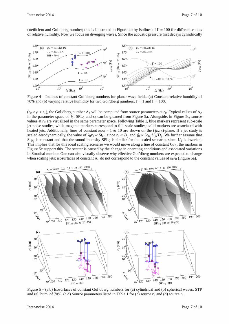
coefficient and Gol’dberg number; this is illustrated in Figure 4bby isolines ofΓ = 100 for different valuesof relative humidity. Now we focus on diverging waves. Sincethe acoustic pressure first decays cylindrically
101
102
103
104120
130
140
150
160
170
180
102
103
104
replacements
f0 (Hz)
SP
L 0(d
Bre
20µP
a)
p rm
s(P
a)
Γ = 10
Γ = 100
Γ = 1,000
(a) p∞ = 101,325 Pa
T∞ = 293.15 K
RH= 70%
101
102
103
104120
130
140
150
160
170
180
102
103
104
f0 (Hz)
SP
L 0(d
Bre
20µP
a)
p rm
s(P
a)
Γ = 100
RH= 0 : 10 : 100%
(b) p∞ = 101,325 Pa
T∞ = 293.15 K
Figure 4 – Isolines of constant Gol’dberg numbers for planarwave fields. (a) Constant relative humidity of70% and (b) varying relative humidity for two Gol’dberg numbers,Γ = 1 andΓ = 100.
(r0 < ρ < r1), the Gol’dberg numberΛc will be computed from source parameters atr0. Typical values ofΛcin the parameter space off0, SPL0 andr0 can be gleaned from Figure 5a. Alongside, in Figure 5c, sourcevalues atr0 are visualized in the same parameter space. Following Table1, blue markers represent sub-scalejet noise studies, while magenta markers correspond to full-scale studies; solid markers are associated withheated jets. Additionally, lines of constantk0r0 = 1 & 10 are shown on the (f0, r0)-plane. If a jet study isscaled aerodynamically, the value ofk0r0 ∝ StD j sincer0 ∝ D j and f0 ∝ StD j U j/D j . We further assume thatStD j is constant and that the sound intensity SPL0 is similar for the scaled scenario, sinceU j is invariant.This implies that for this ideal scaling scenario we would move along a line of constantk0r0; the markers inFigure 5c support this. The scatter is caused by the change inoperating conditions and associated variationsin Strouhal number. One can also visually observe why effective Gol’dberg numbers are expected to changewhen scaling jets: isosurfaces of constantΛc do not correspond to the constant values ofk0r0 (Figure 5a).
Figure 5 – (a,b) Isosurfaces of constant Gol’dberg numbers for (a) cylindrical and (b) spherical waves; STPand rel. hum. of 70%. (c,d) Source parameters listed in Table1 for (c) sourcer0 and (d) sourcer1.
Inter-noise 2014 Page 7 of 10
Page 8 of 10 Inter-noise 2014
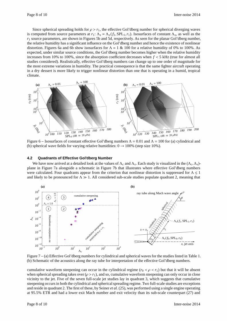
Since spherical spreading holds forρ > r1, the effective Gol’dberg number for spherical diverging wavesis computed from source parameters atr1: Λs = Λs( f1,SPL1, r1). Isosurfaces of constantΛs, as well as ther1 source parameters, are shown in Figures 5b and 5d, respectively. As seen for the planar Gol’dberg number,the relative humidity has a significant influence on the Gol’dberg number and hence the existence of nonlineardistortion. Figures 6a and 6b show isosurfaces forΛ = 1 & 100 for a relative humidity of 0% to 100%. Asexpected, under similar source conditions, the Gol’dberg number becomes higher when the relative humidityincreases from 10% to 100%, since the absorption coefficient decreases whenf < 5 kHz (true for almost allstudies considered). Realistically, effective Gol’dberg numbers can change up to one order of magnitude forthe most extreme variations in humidity. The practical consequence is that the same fighter aircraft operatingin a dry dessert is more likely to trigger nonlinear distortion than one that is operating in a humid, tropicalclimate.
102
103
104 100 110 120 130 140 150 160 170 180
100
101
102
f0 (Hz)
SPL0 (dB re 20µPa)
r 0(c
m)
102
103
104 120 130 140 150 160 170 180 190 200
101
102
103
f1 (Hz)
SPL1 (dB re 20µPa)
r 1(c
m)
Λc = 0.01 Λc = 100Λs= 0.01 Λs= 100(a) (b)
Figure 6 – Isosurfaces of constant effective Gol’dberg numbersΛ = 0.01 andΛ = 100 for (a) cylindrical and(b) spherical wave fields for varying relative humidities: 0→ 100% (step size 10%).
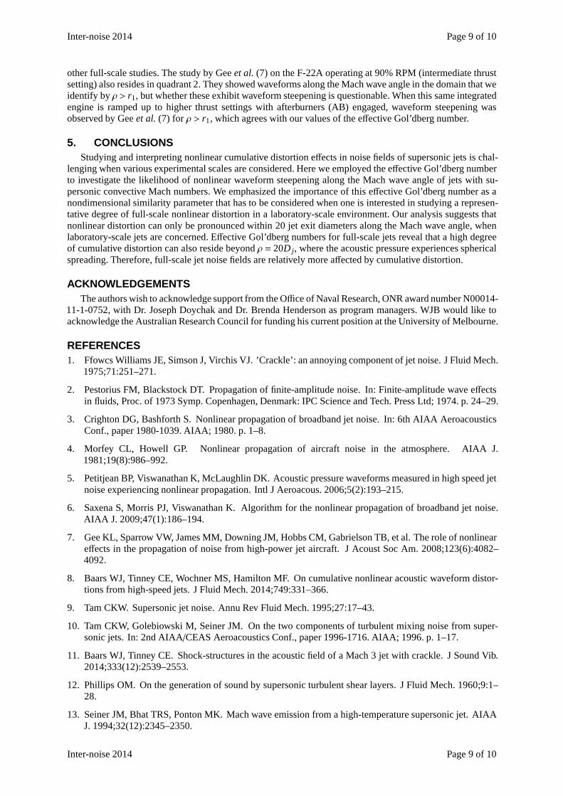
4.2 Quadrants of Effective Gol’dberg NumberWe have now arrived at a detailed look at the values ofΛc andΛs. Each study is visualized in the (Λc,Λs)-
plane in Figure 7a alongside a schematic in Figure 7b that illustrates where effective Gol’dberg numberswere calculated. Four quadrants appear from the criterion that nonlinear distortion is suppressed forΛ . 1and likely to be pronounced forΛ≫ 1. All considered sub-scale studies populate quadrant 2, meaning that
10−1
100
101
102
103
10410
−12
10−10
10−8
10−6
10−4
10−2
100
102
104
Λc
Λs
Λc=
1.0
Λs = 1.0
nocu
mul
ativ
est
ee
peni
ng
cumulative steepening
cum
ulativ
este
epen
ing
restr
icted
toρ<
r 1
x, jet axis
ray tube along Mach wave angle
φ
x= xs
r0
r1
Λs( f1,SPL1, r1)
Λc( f0,SPL0, r0)
cylin
dric
al
sphe
rical
ρ
(a) (b)
1 2
34
Figure 7 – (a) Effective Gol’dberg numbers for cylindrical and spherical waves for the studies listed in Table 1.(b) Schematic of the acoustics along the ray tube for interpretation of the effective Gol’dberg numbers.
cumulative waveform steepening can occur in the cylindrical regime (r0 < ρ < r1) but that it will be absentwhen spherical spreading takes over (ρ > r1), and so, cumulative waveform steepening can only occur in closevicinity to the jet. Five of the seven full-scale jet studieslay in quadrant 3, which suggests that cumulativesteepening occurs in both the cylindrical and spherical spreading regime. Two full-scale studies are exceptionsand reside in quadrant 2. The first of these, by Seineret al.(25), was performed using a single engine operatingat 95.5% ETR and had a lower exit Mach number and exit velocitythan its sub-scale counterpart (27) and
Page 8 of 10 Inter-noise 2014
Inter-noise 2014 Page 9 of 10
other full-scale studies. The study by Geeet al. (7) on the F-22A operating at 90% RPM (intermediate thrustsetting) also resides in quadrant 2. They showed waveforms along the Mach wave angle in the domain that weidentify byρ > r1, but whether these exhibit waveform steepening is questionable. When this same integratedengine is ramped up to higher thrust settings with afterburners (AB) engaged, waveform steepening wasobserved by Geeet al. (7) for ρ > r1, which agrees with our values of the effective Gol’dberg number.
5. CONCLUSIONSStudying and interpreting nonlinear cumulative distortion effects in noise fields of supersonic jets is chal-
lenging when various experimental scales are considered. Here we employed the effective Gol’dberg numberto investigate the likelihood of nonlinear waveform steepening along the Mach wave angle of jets with su-personic convective Mach numbers. We emphasized the importance of this effective Gol’dberg number as anondimensional similarity parameter that has to be considered when one is interested in studying a represen-tative degree of full-scale nonlinear distortion in a laboratory-scale environment. Our analysis suggests thatnonlinear distortion can only be pronounced within 20 jet exit diameters along the Mach wave angle, whenlaboratory-scale jets are concerned. Effective Gol’dberg numbers for full-scale jets reveal that a high degreeof cumulative distortion can also reside beyondρ = 20D j, where the acoustic pressure experiences sphericalspreading. Therefore, full-scale jet noise fields are relatively more affected by cumulative distortion.
ACKNOWLEDGEMENTSThe authors wish to acknowledge support from the Office of Naval Research, ONR award number N00014-
11-1-0752, with Dr. Joseph Doychak and Dr. Brenda Hendersonas program managers. WJB would like toacknowledge the Australian Research Council for funding his current position at the University of Melbourne.
REFERENCES1. Ffowcs Williams JE, Simson J, Virchis VJ. ’Crackle’: an annoying component of jet noise. J Fluid Mech.
1975;71:251–271.
2. Pestorius FM, Blackstock DT. Propagation of finite-amplitude noise. In: Finite-amplitude wave effectsin fluids, Proc. of 1973 Symp. Copenhagen, Denmark: IPC Science and Tech. Press Ltd; 1974. p. 24–29.
3. Crighton DG, Bashforth S. Nonlinear propagation of broadband jet noise. In: 6th AIAA AeroacousticsConf., paper 1980-1039. AIAA; 1980. p. 1–8.
4. Morfey CL, Howell GP. Nonlinear propagation of aircraft noise in the atmosphere. AIAA J.1981;19(8):986–992.
6. Saxena S, Morris PJ, Viswanathan K. Algorithm for the nonlinear propagation of broadband jet noise.AIAA J. 2009;47(1):186–194.
7. Gee KL, Sparrow VW, James MM, Downing JM, Hobbs CM, Gabrielson TB, et al. The role of nonlineareffects in the propagation of noise from high-power jet aircraft. J Acoust Soc Am. 2008;123(6):4082–4092.
8. Baars WJ, Tinney CE, Wochner MS, Hamilton MF. On cumulative nonlinear acoustic waveform distor-tions from high-speed jets. J Fluid Mech. 2014;749:331–366.
9. Tam CKW. Supersonic jet noise. Annu Rev Fluid Mech. 1995;27:17–43.
10. Tam CKW, Golebiowski M, Seiner JM. On the two components of turbulent mixing noise from super-sonic jets. In: 2nd AIAA/CEAS Aeroacoustics Conf., paper 1996-1716. AIAA; 1996. p. 1–17.
11. Baars WJ, Tinney CE. Shock-structures in the acoustic field of a Mach 3 jet with crackle. J Sound Vib.2014;333(12):2539–2553.
12. Phillips OM. On the generation of sound by supersonic turbulent shear layers. J Fluid Mech. 1960;9:1–28.
13. Seiner JM, Bhat TRS, Ponton MK. Mach wave emission from a high-temperature supersonic jet. AIAAJ. 1994;32(12):2345–2350.
Inter-noise 2014 Page 9 of 10
Page 10 of 10 Inter-noise 2014
14. Tam CKW, Chen P. Turbulent mixing noise from supersonic jets. AIAA J. 1994;32(9):1774–1780.
18. Morris PJ. A note on noise generation by large scale turbulent structures in subsonic and supersonic jets.Intl J Aeroacous. 2009;8(4):301–316.
19. Papamoschou D. Wavepacket modeling of the jet noise source. In: 17th AIAA/CEAS AeroacousticsConf., paper 2011-2835. AIAA; 2011. p. 1–20.
20. Baars WJ. Acoustics from high-speed jets with crackle. The University of Texas at Austin. TX; 2013.
21. Fiévet R, Tinney CE, Baars WJ, Hamilton MF. Acoustic waveforms produced by a laboratory scalesupersonic jet. In: 20th AIAA/CEAS Aeroacoustics Conf., paper 2014-2906. AIAA; 2014. p. 1–20.
22. Hileman JI, Thurow BS, Caraballo EJ, Samimy M. Large-scale structure evolution and sound emis-sion in high-speed jets: real-time visualization with simultaneous acoustic measurements. J Fluid Mech.2005;544:277–307.
23. Kuo CW, Veltin J, McLaughlin DK. Effects of jet noise source distribution on acoustic far-field measure-ments. Intl J Aeroacous. 2012;11(7-8):885–915.
24. James MM, Salton AR, Gee KL, Neilsen TB, McInerny SA, Kenny RJ. Modification of directivity curvesfor a rocket noise model. In: 164th Meeting of the ASA., Vol. 18, 040008. ASA; 2014. p. 1–13.
25. Seiner JM, Ukeiley LS, Jansen BJ. Aero-performance efficient noise reduction for the F404-400 engine.In: 11th Aeracoustics Conf., paper 2005-3048. AIAA/CEAS; 2005. p. 1–13.
26. Veltin J, Day BJ, McLaughlin DK. Correlation of flowfield and acoustic field measurements in high-speed jets. AIAA J. 2011;49(1):150–163.
27. Baars WJ, Tinney CE, Murray NE, Jansen BJ, Panickar P. Theeffect of heat on turbulent mixing noisein supersonic jets. In: 49th Aerospace Sciences Meeting, paper 2011-1029. AIAA; 2011. p. 1–14.
28. Bridges JE. Broadband shock noise in internally-mixed dual-stream jets. In: 15th AIAA/CEAS Aeroa-coustics Conf., paper 2009-3210. AIAA; 2009. p. 1–17.
29. Gee KL, Gabrielson TB, Atchley AA, Sparrow VW. Preliminary analysis of nonlinearity in military jetaircraft noise propagation. AIAA J. 2005;43(6):1398–1401. Technical note.
30. Gee KL, Downing JM, James MM, McKinley RC, McKinley RL, Neilsen TB, et al. Nonlinear evolutionof noise from a military jet aircraft during ground run-up. In: 18th AIAA/CEAS Aeroacoustics Conf.,paper 2012-2258. AIAA; 2012. p. 1–13.