Chan Shewiener Nims

November 27, 2005 23:13 WSPC/Lecture Notes Series: 9in x 6in ChanShenIMS

Theory and Computation of Variational Image Deblurring

Tony F. Chan

Department of Mathematics, UCLALos Angeles, CA 90095, USA

E-mail: [email protected]

Jianhong Shen

School of MathematicsUniversity of Minnesota

Minneapolis, MN 55455, USAE-mail: [email protected]

To recover a sharp image from its blurry observation is the problemknown as image deblurring. It frequently arises in imaging sciences andtechnologies, including optical, medical, and astronomical applications,and is crucial for allowing to detect important features and patterns suchas those of a distant planet or some microscopic tissue.

Mathematically, image deblurring is intimately connected to back-ward diffusion processes (e.g., inverting the heat equation), which arenotoriously unstable. As inverse problem solvers, deblurring modelstherefore crucially depend upon proper regularizers or conditioners thathelp secure stability, often at the necessary cost of losing certain high-frequency details in the original images. Such regularization techniquescan ensure the existence, uniqueness, or stability of deblurred images.

The present work follows closely the general framework describedin our recent monograph [18], but also contains more updated viewsand approaches to image deblurring, including, e.g., more discussionon stochastic signals, the Bayesian/Tikhonov approach to Wiener fil-tering, and the iterated-shrinkage algorithm of Daubechies et al. [30,31]for wavelet-based deblurring. The work thus contributes to the devel-opment of generic, systematic, and unified frameworks in contemporaryimage processing.

1


2 Chan and Shen

1. Mathematical Models of Blurs

Throughout the current work, an image u is identified with a Lebesgue

measurable real function on an open two-dimensional (2D) regular domain

Ω. A general point x = (x1, x2) ∈ Ω shall also be called a pixel as in digital

image processing. The framework herein applies readily to color images for

which u could be considered an RGB-vectorial function.

1.1. Linear Blurs

Deblurring is to undo the blurring process applied to a sharp and clear

image earlier, and is thus an inverse problem. We hence start with the

description of the forward problem - mathematical models of blurring.

In most applications, blurs are introduced by three different types of

physical factors: optical, mechanical, or medium-induced, which could lead

to familiar out-of-focus blurs, motion blurs, or atmospheric blurs respec-

tively. We refer the reader to [18] for a more detailed account on the as-

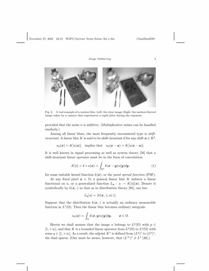
sociated physical processes. Figures 1 and 2 show two real blur examples

directly taken by a digital camera under different circumstances.

Fig. 1. A real example of an out-of-focus blur. Left: the clear image; Right: the out-of-focus image taken by a digital camera that focuses on a point closer than the scene.

Mathematically, blurring can be either linear or nonlinear. The latter is

more challenging to invert due to the scarcity of proper nonlinear models.

The current work shall mainly focus on linear deblurring problems.

A general linear blur u0 = K[u] is defined by a linear operator K. In

most applications noise is unavoidable and a real observation is thus often

modelled by

u0 = K[u] + n,


Image Deblurring 3

Fig. 2. A real example of a motion blur. Left: the clear image; Right: the motion-blurredimage taken by a camera that experiences a rapid jitter during the exposure.

provided that the noise n is additive. (Multiplicative noises can be handled

similarly.)

Among all linear blurs, the most frequently encountered type is shift-

invariant. A linear blurK is said to be shift-invariant if for any shift a ∈ R2,

u0(x) = K[u(x)] implies that u0(x − a) = K[u(x − a)].

It is well known in signal processing as well as system theory [56] that a

shift-invariant linear operator must be in the form of convolution:

K[u] = k ∗ u(x) =

∫

R2

k(x − y)u(y)dy, (1)

for some suitable kernel function k(x), or the point spread function (PSF).

At any fixed pixel x ∈ Ω, a general linear blur K induces a linear

functional on u, or a generalized function Lx : u → K[u](x). Denote it

symbolically by k(x, ·) so that as in distribution theory [68], one has

Lx[u] = 〈k(x, ·), u(·)〉.

Suppose that the distribution k(x, ·) is actually an ordinary measurable

function in L1(Ω). Then the linear blur becomes ordinary integrals:

u0(x) =

∫

Ω

k(x,y)u(y)dy, x ∈ Ω.

Herein we shall assume that the image u belongs to Lp(Ω) with p ∈[1,+∞], and that K is a bounded linear operator from Lp(Ω) to Lq(Ω) with

some q ∈ [1,+∞]. As a result, the adjointK∗ is defined from (Lq)∗ to (Lp)∗,

the dual spaces. (One must be aware, however, that (L∞)∗ 6= L1 [48].)


4 Chan and Shen

1.2. The DC-Condition

The most outstanding characteristic of a blur operator is the DC-condition:

K[1] = 1, treating 1 ∈ L∞(Ω). (2)

In classical signal processing [56], DC stands for direct current since the

Fourier transform of a constant contains no oscillatory frequencies. By du-

ality, 〈K[u], v〉 = 〈u,K∗[v]〉, and the DC-condition on K amounts to the

mean-preserving condition on K∗:

〈K∗[v]〉 = 〈v〉, by setting u = 1; or

∫

Ω

K∗[v](x)dx =

∫

Ω

v(x)dx,

(3)

if both v and K∗[v] belong to L1(Ω).

In terms of information theory [27], the DC condition implies that con-

stant signals are invariant under blurring. In particular, blurs cannot gen-

erate ripples from flat signals, and thus can never create information.

When the blur is shift-invariant with a PSF k, the DC-condition requires∫

R2

k(x)dx = 1, or in terms of its Fourier transform, K(ω = 0) = 1,

since the adjoint is also shift-invariant with PSF k(−x). Moreover, a more

convincing blur operator has to be lowpass [56,67], i.e., K(ω) must decay

rapidly at high frequencies.

1.3. Nonlinear Blurs

Blurs could be nonlinear, though linear models prevail in the literature.

Consider for example the following nonlinear diffusion model:

vt = ∇ ·[

1√

1 + |∇v|2∇v

]

, v∣

∣

t=0= u(x). (4)

Let the solution be denoted by v(x, t). For any fixed finite time T > 0,

define a nonlinear operator K = KT by: u0 = K[u] = v(x, T ). Nonlinearity

is evident since for example K[λu] 6= λK[u] for general u and λ 6= 0. But

the operator K apparently satisfies the DC-condition. Furthermore, (4) is

the gradient descent equation of the minimum surface energy

E[v] =

∫

R2

√

1 + |∇v|2dx.

As a result, the above nonlinear diffusion model always smoothens out any

rough initial surfaces. In particular, small scale features and oscillations of u


Image Deblurring 5

must be wiped out in u0 = K[u], making u0 a visually blurred and mollified

version of the original image u. Notice remarkably that the nonlinear blur

is in fact shift-invariant.

2. Illposedness of Deblurring

The illposedness of deblurring could be readily understood in four intrigu-

ing aspects. Understanding the root and nature of illposedness helps one

design good deblurring models. The following four viewpoints are in some

sense the four different facets of a same phenomenon, and hence must not

be taken individually.

A. Deblurring is Inverting Lowpass Filtering. In the Fourier domain,

a blur operator is often lowpass so that high frequency details are com-

pressed by vanishing multipliers. As a result, to deblur a blurry image, one

has to multiply approximately the reciprocals of the vanishing multipliers,

which is conceivably unstable to noises or other high-frequency perturba-

tions in the image data.

B. Deblurring is Backward Diffusion. By the canonical PDE theory,

to blur an image with a Gaussian kernel amounts to running the heat

diffusion equation for some finite duration with the given image as the

initial data. Therefore, to deblur is naturally equivalent to inverting the

diffusion process, which is notoriously unstable.

Stochastically, diffusion corresponds to the Brownian motions of an ini-

tial ensemble of particles. Thus to deblur or to de-diffuse amounts to revers-

ing an irreversible random spreading process, which is physically illposed.

C. Deblurring is Entropy Decreasing. The goal of deblurring is to re-

construct the detailed image features from a mollified blurry image. Thus

from the standpoint of statistical mechanics, deblurring is a process to in-

crease (Shannon) information, or equivalently, to decrease entropy. Accord-

ing to the second law of statistical mechanics [41], deblurring thus could

never occur naturally and extra work has to be done to the system.

D. Deblurring is Inverting Compact Operators. In terms of abstract

functional analysis, a blurring process is typically a compact operator. A

compact operator is one that maps any bounded set (according to the


6 Chan and Shen

associated Hilbert or Banach norms) to a much better behaved set which is

precompact. To achieve this goal, intuitively speaking, a compact operator

has to mix spatial information or introduce many coherent structures, which

is often realized essentially by dimensionality reduction based on vanishing

eigenvalues or singular values. Therefore to invert a compact operator is

again equivalent to de-correlating spatial coherence or reconstructing the

formerly suppressed dimensions (during the blurring process) of features

and information, which is unstable.

This illustration can be further vivified via finite-dimensional linear al-

gebra [65,66]. Looking for an unknown vector u of dimension much higher

than its observation b for the matrix-vector equation Au = b often has

either no solution or infinitely many. Any unique meaningful solution has

to be defined in some proper way.

3. Tikhonov and Bayesian Regularization

From the above discussion, proper regularization techniques have to be

sought after in order to alleviate the illposedness of the deblurring process.

Two universal regularization approaches, which are essentially recipro-

cal in the two dual worlds of deterministic and stochastic methodologies, are

Tikhonov regularization [69] and the Bayesian inference theory [45]. Their

intimate connection has been explained in, for example, Mumford [53], and

Chan, Shen, and Vese [20].

In essence, both approaches introduce some prior knowledge about the

target images u to be reconstructed. In the Bayesian framework, it is to

introduce some proper probability distribution over all possible image can-

didates, and necessary bias (i.e., regularization) is encouraged to favor more

likely ones. In the Tikhonov setting, the prior knowledge is often reflected

through some properly designed “energy” formulations, e.g., a quadratic

energy like a‖u‖2 under some proper functional norm.

We now introduce the most general framework of Baysian-Tikhonov

regularization for deblurring. Consider the blur model

u0(x) = K[u](x) + n(x), x = (x1, x2) ∈ R2,

with a general blur operator K and additive white noise n.

First, assume that blur processK is either known explicitly or estimated

in advance [18]. As an estimation problem, deblurring can be carried out

by the Bayesian principle or MAP (maximum a posteriori probability):

u = argmaxProb(u | u0,K),


Image Deblurring 7

or equivalently, in terms of the logarithmic likelihood or Gibbs’ ensemble

formula E[·] = − log p(·) + a constant or fixed free energy [24],

u = argminE[u | u0,K].

The Bayesian formula with a known blur K is given by

Prob(u | u0,K) = Prob(u | K)Prob(u0 | u,K)/Prob(u0 | K).

Given an image observation u0, the denominator is simply a fixed prob-

ability normalization constant. Thus effectively one seeks an estimator u

to minimize the product of the prior model Prob(u | K) and the data (or

fidelity) model Prob(u0 | u,K). Since ideal images and blurs are often inde-

pendent, one has Prob(u | K) = Prob(u). Therefore in terms of the energy

formulation, one attempts to minimize the posterior energy

E[u | u0,K] = E[u] +E[u0 | u,K]. (5)

In the setting of Tikhonov regularization, the prior energy E[u] is virtually

a regularizer for the data fitting model E[u0 | u,K]. Functionally, E[u] can

be specified by a suitable norm or semi-norm in some proper function space

such as the BV or Besov spaces, which will be discussed later.

For blind deblurring when the kernel K is unknown, the Bayesian for-

mula becomes

maxu,K

Prob(u,K | u0) = Prob(u0 | u,K)Prob(u,K)/p(u0).

In most applications, the blur mechanism K is uncorrelated to the image

content u (e.g., in astronomical imaging, atmospheric turbulence activities

K are not influenced by the ideal image observation u of the stars and

galaxies many lightyears away). Then one has

Prob(u,K) = Prob(u)Prob(K),

and the posterior energy takes the form of

E[u,K | u0] = E[u0 | u,K] +E[u] +E[K], (6)

up to a fixed additive constant (corresponding to the free energy under the

given parameters in the models).

In both models (5) and (6) for non-blind and blind deblurring, the data

generation model E[u0 | u,K] is often readily expressible via squared fitting

error for Gaussian white noise. Thus the key to effective deblurring relies

upon the proper proposals on the prior knowledge for the target image u,

as well as the blur process K in the blind scenario.


8 Chan and Shen

4. Optimal Wiener Filtering for Non-Blind Deblurring

From now on, instead of the black-faced symbols x and ω, a general pixel

will be denoted by x = (x1, x2) and its frequency dual variable by ω =

(ω1, ω2). Due to the stochastic nature of Wiener filtering, we shall begin

with a brief introduction to 2-D stochastic signals.

4.1. 2-D Stochastic Spatial Signals

Consider only real stochastic images defined on the domains of either R2

for analog images or the lattice Z2 for digital ones.

A stochastic image u(x) is said to be homogeneous if any of its finite

marginal distributions carries no spatial memory, or equivalently, is trans-

lation invariant:

Px+z,··· ,y+z(u, · · · , v) ≡ Px,··· ,y(u, · · · , v), ∀z = (z1, z2),

where the marginal probability is defined by

Px,··· ,y(u, · · · , v)du · · · dv = Prob(u(x) ∈ [u, u+du], · · · ,u(y) ∈ [v, v+dv]).

Familiar sources for homogenous images include Gibbs’ random fields with

translation invariant potentials, or Markov random fields with translation

invariant graph structures and local conditionals [6,18,40]. Homogeneity is

appropriate for modelling certain ideal single-species textures such as sandy

beaches or grasslands, which are more or less uniform.

More generally, a stochastic signal u is said to be wide-sense homoge-

neous (WSH), if its two-point auto-correlation function

Ruu(x, y) = E[u(x)u(y)],

is translation invariant: for any relocation z,

Ruu(x+ z, y + z) = Ruu(x, y).

Thus if u is WSH, its auto-correlation function is essentially a single-pixel

function: Ruu(x − y) = Ruu(x, y). Let ω = (ω1, ω2) denote the spatial

frequency variable. Then the power spectral density Suu(ω) is defined to

be the Fourier transform of Ruu(x):

Suu(ω) =

∫

R2

Ruu(x)e−ixωdx.

A WSH image n(x) is said to be white noise, if Snn(ω) ≡ σ2, or equiva-

lently, its auto-correlation function Rnn(x) is a constant multiple of Dirac’s

delta signal δ(x).


Image Deblurring 9

Two WSH images u and v are said to be cross-WSH if their cross-

correlation function is translation invariant as well.

Ruv(x, y) = E[u(x)v(y)] = Ruv(x− y). (7)

Define the cross-WSH set of a given WSH image u to be

Λu = v | v is cross-WSH to u . (8)

Then u ∈ Λu. Furthermore, we have the following list of straightforward

but useful properties.

Theorem 1: Suppose u is WSH and Λu its cross-WSH set. Then Λu is a

linear space which is closed under spatial relocation:

v(·) ∈ Λu ⇒ v(· + z) ∈ Λu,

for any relocation z ∈ R2, as well as under linear filtering:

v ∈ Λu ⇒ h ∗ v ∈ Λu,

for any filter h = h(x). Let H(ω) denote the impulse response of h. Then,

Rh∗v,u(x) = h ∗Rvu(x), and Sh∗v,u(ω) = H(ω)Svu(ω).

4.2. Stochastic Signals as Random Generalized Functions

Another intriguing approach to stochastic signals is to treat a stochastic

signal as a random generalized function.

Recall that a generalized function F , or a Schwartz distribution, is a

linear functional on the test function space D = C∞0 (R2), so that for any

test function φ ∈ D,

the determinisitc values 〈F, φ〉 are linear in φ.

A 2D stochastic field u on R2 can be treated as a random generalized

function so that for any test function φ ∈ D, the value

Uφ = 〈u, φ〉 is a random variable, and Uaφ+bψ = aUφ + bUψ.

The mean field of u is an ordinary generalized function mu such that

E(Uφ) = 〈mu, φ〉, for any φ ∈ D.

If mu = 0, u is said to have zero means. Two random fields u and v are

said to be equivalent if Uφ and Vφ share the same probability distribution

for any test function φ ∈ D.


10 Chan and Shen

For any shifting operator Sz : φ(x) → φ(x− z) with z ∈ R2, the shifted

random field Szu is defined by the dual formula

〈Szu, φ〉 = 〈u, S−zφ〉, φ ∈ D.

u is said to be shift invariant if u is equivalent to Szu for any shift z. If a

test function φ is interpreted as a measurement sensor, then a random field

is shift invariant if and only if no statistical difference can be detected from

the measurements when a sensor is moved from one location to another.

A random field u of zero means is said to be wide-sense homogeneous

(WSH) if there exists some locally integrable function Ruu(x) such that for

any two test functions φ and ψ, one has

E(UφUψ) = 〈φ,Ruu ∗ ψ〉.

Similarly, two random fields u and v of zero means are said to be cross-

WSH if there exists some locally integrable function Ruv(x) such that for

any test functions φ and ψ,

E(UφVψ) = 〈φ,Ruv ∗ ψ〉.

Ruu and Ruv are called the auto-correlation and cross-correlation func-

tions, and are apparently unique if in existence. If one formerly takes Dirac’s

delta functions as test functions, it is easy to verify the consistency between

the current functional definitions and the pointwise definitions in the pre-

ceding subsection.

The reader can familiarize the above theory with the help of the follow-

ing example of random harmonic waves in 1D:

u(x) = A cos(x+B), x ∈ R,

where A and B are independent random variables with B uniformly dis-

tributed over [0, 2π), and A exponentially distributed on (0,∞). Then it is

easy to show, for example, that u must be homogenous (or shift invariant).

4.3. Filtering-Based Deblurring

Assume that the blur is shift invariant: u0 = k ∗ u + n. Filtering-based

deblurring is to produce an estimator u of the ideal image u via a linear

filtering scheme:

u = uw = w ∗ u0, with a suitable filter w.

Without noise, the ideal filter would be directly given by W (ω) = 1K(ω) ,

in the Fourier domain, so that u = w ∗ u0 ≡ u for any clear image u and


Image Deblurring 11

perfect reconstruction is reached! However, it is a rather unnerving formula

since a typical blur k is often lowpass and K(ω) decays rapidly at high

frequencies. Such a naive filter therefore exaggerates any high-frequency

errors or perturbations.

To alleviate such unwanted instability, in the noise-free case one rewrites

the naive filter W = 1/K to

W (ω) =K∗(ω)

K(ω)K∗(ω)=

K∗

|K|2 , where ∗ denotes complex conjugacy.

The vanishing denominator at high frequencies can be guarded away from

zero by incorporating a positive factor r = r(ω):

W →Wr =K∗

|K|2 + r. (9)

The resultant deblurred image ur is then given by

ur = wr ∗ k ∗ u,

or in the Fourier domain, the composite effect of the blurring and deblurring

processes is achieved by the multiplier

Wr(ω)K(ω) =|K(ω)|2

|K(ω)|2 + r(ω). (10)

The restoration indeed well approximates the identity operator on low fre-

quencies where r |K|2 since K is lowpass. High frequencies are however

suppressed since K almost vanishes and |K|2 r. Thus the regularizer r

plays a soft cutoff role.

The reader should pay constant attention to the frequent emergency of

such an r-factor henceforth. It embodies a universal quantity that is critical

for any deblurring problem.

The question is how to choose wisely an optimal regularizer r. A uniform

constant is a reasonable guess but lacks clear theoretical backup. What

Wiener discovered was that r should be related to the signal-to-noise ratio

in the observation u0, which will be explained in the next subsection.

It is also the right spot to reiterate the earlier analogy drawn from

the finite linear algebra of solving Au = b. Recall that the least square

solution [65,66] is given by the normal equation:

A∗Au = A∗b, or u = (A∗A)−1A∗Au.

Thus the “filter” in the least-square solution is given by

W = (A∗A)−1A∗.


12 Chan and Shen

When the linear operator A “mixes” information too intensely so that

rank (A) = dim(Range(A)) # of rows of A,

A∗A becomes singular (or almost singular if the approximate rank only

counts the nonnegligible singular values of A). Then the inversion of

(A∗A)−1 still remains illposed or unstable. In linear algebra, the filter is

then regularized to

Wr = (A∗A+ rI)−1A∗ (11)

for some positive small parameter r > 0, where I is the identity matrix. The

resultant estimator corresponds to the regularized least-square problem:

ur = argminu‖Au − b‖2 + r‖u‖2.

Notice the characteristic similarity between (9) and (11).

4.4. Optimal Wiener Filtering

Wiener’s filter w is to minimize the mean squared estimation error ew de-

fined by ew(x) = uw(x) − u(x). That is,

w = argminhE(e2h) = argminhE(h ∗ u0(x) − u(x))2. (12)

Notice that Wiener’s filter is independent of the particular pixel x used in

the above definition since eh is easily seen to be WSH for any fixed real filter

h = h(x), provided that u the ideal image and n the noise are independent

and WSH.

Variation on the optimal Wiener filter: w → w + δh gives the “equilib-

rium” equation

E[(w ∗ u0(x) − u(x)) (δh ∗ u0(x))] = 0.

Taking localized small variation δh(x) = εδ(x − a) for some ε 1 at any

site a, one can rewrite the equation to E[(w ∗ u0(x) − u(x))u0(x− a)] = 0.

Since a is arbitrary, it is equivalent to

E[(w ∗ u0(x) − u(x))u0(y)] = 0, ∀x, y ∈ Ω, (13)

the one known as the orthogonal condition for Wiener’s filter.

By Theorem 1, in terms of the correlation functions, one has

w ∗Ru0u0(z) = Ruu0

(z), z ∈ R2.


Image Deblurring 13

The optimal Wiener filter is thus given by W (ω) = Suu0(ω)/Su0u0

(ω),

expressed in terms of the power spectral densities. For the blur model:

u0 = k ∗ u+ n, one has, according to Theorem 1,

Suu0= K∗(ω)Suu(ω), and Su0u0

= |K(ω)|2Suu(ω) + Snn(ω).

Therefore, we have established the following theorem.

Theorem 2: (Wiener Filter for Deblurring) The optimal Wiener filter is

given by, in the Fourier domain,

W (ω) =K∗Suu

|K|2Suu + Snn=

K∗

|K|2 + rw, (14)

where the regularizer rw = Snn/Suu is the squared noise-to-signal ratio.

For a Gaussian white noise with variance σ2, one has Snn(ω) ≡ σ2. Since

Suu is often bounded, the Wiener regularizer rw is therefore well bounded

above zero.

We refer the reader to, e.g., [43,47] for further improvement of the above

classical Wiener filters, especially on relaxing the stochastic assumptions on

the signals and the conditions on the blur model.

4.5. Connection to the Bayesian/Tikhonov Method

We now show that Wiener filtering is intimately connected to the general

framework of Bayesian or Tikhonov regularization laid out in the preceding

section.

Take the quadratic data-fitting model

E[u0 | u, k] = λ‖k ∗ u− u0‖2 = λ

∫

R2

(k ∗ u− u0)2dx

for additive Gaussian white noise, where λ is inversely proportional to the

noise variance σ2.

For the prior model E[u], assume the ideal image u belongs to the

fractional-Sobolev space Hγ(R2). Formally, this means that u ∈ L2(R2)

and its fractional gradient ∇γu ∈ L2(R2). More rigorously, the norm is

properly defined in the Fourier domain by:

‖u‖2γ =

∫

R2

(1 + |ω|2)γ |U(ω)|2dω,

where U(ω) denotes the Fourier transform of u(x). Define

r(ω) =(1 + |ω|2)γ

λ=

λ−1

(1 + |ω|2)−γ . (15)


14 Chan and Shen

Notice that r(ω) can indeed be considered as the squared noise-to-signal

ratio as in the Wiener filter since λ−1 is proportional to the noise variance

and the denominator is proportional to the squared signal strength. (More

precisely, the noise n has been assumed in L2 and its power spectral density

is the ideal variance σ2 modulated by some decay factor |ω|−2α, which is

however shared by the signal and cancelled out. This makes the above r a

more authentic squared noise-to-signal ratio.)

Notice that the power-law decay in (15) is very common in stochastic

signal analysis and processing.

One is thus led to the following posterior energy for deblurring:

E[u | u0, k] = λ‖k ∗ u− u0‖2 + ‖u‖2γ.

In the Fourier domain, it is equivalent to the energy

E[U | U0,K] =

∫

Ω

|K(ω)U(ω) − U0(ω)|2 dω +

∫

Ω

r(ω)|U(ω)|2dω. (16)

Performing variation on U , one has the equilibrium equation for the optimal

estimator:

K∗(KU − U0) + rU = 0, or U(ω) =K∗(ω)

|K|2(ω) + r(ω)U0(ω),

with r being the squared noise-to-signal ratio. This could be considered as

the deterministic version of Wiener filtering. To our best knowledge, such

an explicit connection has never been made before in the literature.

More generally, with r(ω) already computed for Wiener filtering (14),

one can substitute it into the Bayesian/Tikhonov formulation (16), and

arrive at the precise posterior energy form for deterministic Wiener filtering.

An interesting case occurs if r(ω) = (1+ |ω|2)−µ for some notable µ > 0,

which corresponds to the scenario when the target image signal u is highly

oscillatory, or is functionally a generalized function instead of L2 [64].

5. Deblurring Blurred BV Images

One of the most powerful deterministic image prior model is the space of

functions of bounded variations BV(Ω), first introduced into image process-

ing by Rudin, Osher, and Fatemi [61]. In this section, we discuss the theory

and computation of deblurring BV images.

5.1. TV Deblurring by Rudin, Osher, and Fatemi

The total variation (TV) of a BV image u is conventionally denoted by∫

Ω |Du| or |Du|(Ω) [38,42]. When the image u is smooth so that its gradient


Image Deblurring 15

∇u belongs to L1, the TV is simply the ordinary L1 integral∫

Ω

|Du| =

∫

Ω

|∇u|dx,

in the sense of Sobolev norm. For a more generic BV image u that has

discontinuous jumps, the TV |Du| is in fact a Radon measure so that for

any open set Q ⊂ Ω,

|Du|(Q) = supg∈C1

0(Q,B2)

∫

Q

u(∇ · g)dx,

where B2 ⊂ R2 denotes the unit open disk centered at the origin and g =

(g1, g2) is vectorial. For more introduction to BV images and their applica-

tions in image analysis and processing, we refer the reader to our new mono-

graph [18], the more mathematically oriented monographs [38,42], as well

as numerous existent works, e.g., [1,7,9,12,16,17,50,57,58,62,63,70,71,72].

In one adopts the TV measure for image regularization: E[u] =

α∫

Ω |Du|, the posterior energy for Bayesian/Tikhonov deblurring then

takes the form of

E[u | u0, k] = E[u] +E[u0 | u, k]

= α

∫

Ω

|Du| + λ

2

∫

Ω

(k ∗ u− u0)2dx,

(17)

with x = (x1, x2) ∈ Ω = R2 and two suitable positive weights α and λ. This

was the restoration model originally proposed and computed by Rudin-

Osher-Fatemi [60,61], and later further studied by many others [9,72,73].

Notice that as far as energy minimization is concerned, only the ratio

r = α/λ contributes to the solution process. As for parametric estimation

in statistics, one could also treat r as an unknown as well, and expand the

energy to E[u, r | u0, k] by absorbing some prior knowledge E[r] on r.

The previous discussion on the optimal Wiener filtering (14) seems to

suggest that the ratio r = α/λ is in the same dimension of the noise-to-

signal ratio rw. In particular, r should be proportional to the variance σ2 of

the noise, which is natural since by the Bayesian rationale for least square

fidelities, one indeed has λ = O(1/σ2).

5.2. Dealing With Bounded Image Domains

In model (17), it has been conveniently assumed that the image domain

Ω is the entire plane R2 to facilitate shift invariance. In real applications,


16 Chan and Shen

however, Ω is often a bounded disk or square for which the blur

K[u] = k ∗ u(x) =

∫

R2

k(x− y)u(y)dy, x ∈ Ω

needs to be properly redefined.

First, one can remodify the blur to a shift-variant PSF given by

k(x, y) =k(x− y)

∫

Ωk(x− z)dz

, ∀x, y ∈ Ω. (18)

We assume that the original PSF k(x) is nonnegative, and x = (0, 0) belongs

to the support of the measure dµ(x) = k(x)dx. That is, the integral of k(x)

on any neighborhood of (0, 0) is positive. Then the denominator in (18) is

always positive. It is also easy to see that the DC-condition K[1] = 1 still

holds after the modification.

An alternative way is to first extrapolate u beyond Ω. Let

Q : u∣

∣

Ω→ u = Q[u]

∣

∣

R2,

be a suitable linear extrapolation operator which extends u on Ω onto the

entire plane. (Functionally, Q could be some linear operator from, e.g.,

W 1,∞(Ω) to W 1,∞(R2).) Then the blur is modified to

K[u](x) = k ∗ u(x) = k ∗Q[u](x), ∀x ∈ Ω, (19)

or equivalently, K = 1Ω · (k ∗Q) with a multiplier 1Ω(x).

The DC-condition is satisfied if and only if k ∗Q[1] ≡ 1 when restricted

in Ω. In particular, the natural condition Q[1] ≡ 1 would suffice since k

satisfies the DC-condition on R2.

If Q is represented by some kernel g(x, y) with y ∈ Ω, x ∈ R2. Then the

modified K is represented by

k(x, y) =

∫

R2

k(x− z)g(z, y)dz, x, y ∈ Ω.

Therefore the DC-condition is satisfied when g and k meet the following

compatibility condition∫

Ω

∫

R2

k(x− z)g(z, y)dzdy ≡ 1, ∀x ∈ Ω. (20)

Finally, another less traditional approach to handling bounded domains

can be based on the inpainting technique [4,5,11,13,14,15,16,17,19,36]. Sup-

pose that k(x) is compactly supported on a disk Bρ(0) = x ∈ R2 : |x| < ρ,

and the ρ-neighborhood of Ω is defined by

Ωρ = x ∈ R2 | dist(x,Ω) < ρ.


Image Deblurring 17

Assume also the ideal image u ∈ BV(Ω). Then, instead of the original

model (17), one can attempt to minimize the modified version –

E[u | u0, k, ρ] = α

∫

Ωρ

|Du| + λ

2

∫

Ω

(k ∗ u− u0)2dx. (21)

The convolution inside the fidelity term no longer stirs up any problem.

In summary, both the restricted-kernel method (18) and the image-

extrapolation method (19) lead to a shift-variant blur K with kernel k(x, y),

and the deblurring model for BV images becomes

minuETV[u | u0,K] = α

∫

Ω

|Du| + λ

2

∫

Ω

(K[u] − u0)2dx. (22)

Next we briefly discuss the solutions to this model. More details can be

found, for example, in [1,9,18].

5.3. Existence and Uniqueness

Following the preceding preparation, the image domain Ω can be assumed

bounded and Lipschitz in R2. In addition, we assume that (i) the ideal

image u ∈ BV(Ω), (ii) the blurry and noisy observation u0 ∈ L2(Ω), and

(iii) the linear blur K : L1(Ω) → L2(Ω) is bounded, injective, and satisfies

the DC-condition: K[1] ≡ 1.

Condition (i) and (ii) are necessary for (22) to be well defined. Injectivity

in (iii) is also necessary for the uniqueness of optimal deblurring.

The proof for the following theorem can be found in, e.g., [9,18].

Theorem 3: (Existence and Uniqueness of BV Deblurring) Under the pre-

ceding three conditions, the optimal deblurring u∗ = argminE[u | u0,K]

for model (22) exists and is unique.

Furthermore, the unique minimizer must satisfy the mean constraint.

Corollary 4: (The Mean Constraint) The unique minimizer u∗ must au-

tomatically satisfy the mean constraint 〈K[u∗]〉 = 〈u0〉.

Stochastically, this is a natural inference from the blur model

u0 = K[u] + n,

since the noise has zero means. Deterministically, this fact has to be proven

from the deblurring model.


18 Chan and Shen

Proof: For the unique minimizer u∗, define for any c ∈ R

e(c) = E[u∗ − c | u0,K].

Then c∗ = argmin e(c) has to minimize∫

Ω

(K[u∗] − u0 − c)2dx, since K[c] = c.

As a result, the unique minimizer c∗ = 〈K[u∗]− u0〉. On the other hand c∗has to be zero since u∗ − c∗ = u∗ due to uniqueness. Therefore,

〈K[u∗]〉 = 〈u0〉,

which establishes the assertion.

Figures 3, 4, and 5 are three generic examples from [18] that demonstrate

the performance of the deblurring model (22).

an out−of−focus image deblurred image (with known PSF)

Fig. 3. Deblurring an out-of-focus image.

5.4. Computation and Examples

The variational deblurring model (22) has been computed more or less

based on the formal Euler-Lagrange equation [1,9,60,61]:

α∇ ·[ ∇u|∇u|

]

− λK∗[K[u]− u0] = 0, (23)


Image Deblurring 19

image blurred by horizontal hand jittering deblurred image (with known PSF)

Fig. 4. Deblurring a motion-blurred image.

image blurred by horizontal hand jittering deblurred image (with known PSF)

Fig. 5. Restoring another motion-blurred image.

with Neumann adiabatic condition ∂u/∂n = 0 along the boundary ∂Ω.

Equation (23) holds in the distributional sense, i.e., for any compactly sup-

ported smooth test function φ, the solution satisfies

α〈∇φ, ∇u|∇u| 〉 + λ〈K[φ],K[u] − u0〉 = 0.

The nonlinear degenerate elliptic equation (23) is often regularized to

α∇ ·[ ∇u|∇u|a

]

− λK∗[K[u] − u0] = 0, (24)

where the notation |x|a denotes√x2 + a2 for some fixed positive parameter


20 Chan and Shen

a. It amounts to minimizing

E[u | u0,K, a] = α

∫

Ω

√

|Du|2 + a2 +λ

2

∫

Ω

(K[u] − u0)2dx, (25)

which is closely connected to the minimal surface problem [42].

Computationally, the most common algorithm has been based on the so-

called lagged-diffusivity technique [9,18,72], which is an iterative procedure.

Based on the current best estimation u(n), one solves for u(n+1) the following

linearized equation:

α∇ ·[∇u(n+1)

|∇u(n)|a

]

− λK∗[K[u(n+1)] − u0] = 0, (26)

with the Neumann condition. Notice that given u(n), the linear operator

Ln = −α∇ · 1

|∇u(n)|a∇ + λK∗K

is positive definite or strictly elliptic.

This algorithm guarantees convergence since it is equivalent to the

alternating-minimization (AM) algorithm for the augmented energy

Ea[u, z | u0,K] =α

2

∫

Ω

(

z|∇u|2 + z−1)

dx+λ

2

∫

Ω

(K[u] − u0)2dx,

where z = z(x) is an auxiliary field, which corresponds to the edge signature

function in image processing [17]. Then it can be easily shown that

minu,z

Ea[u, z | u0,K] = minuETV[u | u0,K].

Furthermore, the above lagged-diffusivity algorithm corresponds to exactly

the AM algorithm for the augmented energy:

· · · → u(n) → z(n) → u(n+1) → · · · .

6. Parametric Blind Deblurring

In all the above models, the blur K has been assumed known. We now

develop variational deblurring models when the blur is unknown, a sce-

nario often nicknamed “blind deblurring” [39,46,75]. Inspired by the theory

of statistical estimation, we shall classify such models into ones that are

parametric or nonparametric, or figuratively, partially blind or completely

blind.


Image Deblurring 21

6.1. Parametric Modeling

Suppose that the unknown linear blur belongs to a known parametric family

K = Kθ | θ ∈ I ⊂ Rd,

where θ = (θ1, · · · , θd) denotes a d-dimensional parametric vector and varies

on a subset or domain I in Rd. One is therefore not completely “blind” to the

blur operator, and the uncertainty only arises from θ. A familiar example

is the Gaussian family of shift-invariant blurs Kθ = g∗ given by

g(x | θ) =1

2πθexp

(

−x21 + x2

2

2θ

)

, θ ∈ I = (0,∞), (27)

where in statistics θ precisely corresponds to the variance σ2.

By the Bayesian rationale stated previously [18,53], parametric blind

deblurring becomes the minimization of

E[u, θ | u0] = E[u0 | u, θ] +E[u] +E[θ]. (28)

The first two terms can be safely copied from the non-blind deblurring

model discussed previously. Thus it suffices to incorporate some appropriate

model for the parameter distribution p(θ) or E[θ].

Suppose u ∈ BV(Ω), θ ∈ I ⊂ Rd, and E[θ] = φ(θ) for some suitable

function φ. Then the deblurring model is explicitly given by

E[u, θ | u0] = α

∫

Ω

|Du| + λ

2

∫

Ω

(Kθ[u] − u0)2dx+ φ(θ). (29)

Assume that φ(θ) is bounded below: φ(θ) ≥ M > −∞ for all θ ∈ I .

Otherwise it can attenuate the role of the first two terms in (29) and distort

the real intention of the model. As an example, consider the Gaussian family

in (27). Suppose the variance θ is subject to the exponential distribution

with density function:

p(θ) = a exp(−aθ), θ ∈ I = (0,∞), for some a > 0. (30)

Then φ(θ) = E[θ] = − ln p(θ) = aθ − ln a ≥ − lna > −∞.

Following Theorem 3, Kθ is assumed to be injective and satisfy the

DC-condition Kθ[1] = 1. Then for any given θ, the conditional minimizer

uθ = argminE[u | u0,Kθ] = argminα

∫

Ω

|Du|+ λ

2

∫

Ω

(Kθ[u]−u0)2dx (31)

always exists and is unique by Theorem 3. The original model (29) is then

reduced to an optimization problem on the parameter domain I ⊂ Rd:

minθ∈I

e(θ), with e(θ) = E[uθ, θ | u0].


22 Chan and Shen

e(θ) is, however, generally non-convex and consequently the global mini-

mizer (uθ∗ , θ∗) could be non-unique.

6.2. The AM Algorithm

Such a multivariable optimization problem can usually be solved by the

alternating-minimization (AM) algorithm [2,3,18,22,23,36,54]. One starts

with some initial guess θ(0), which could be drawn from argminφ(θ) for

instance. Then, one successively obtains the alternating conditional mini-

mizers

θ(0) → u(0) → θ(1) → u(1) → · · · (32)

by optimizing the conditional energies:

u(n) = argminE[u | u0, θ(n)], followed by

θ(n+1) = argminE[θ | u0, u(n)], where

E[θ | u0, u] =λ

2

∫

Ω

(Kθ[u] − u0)2dx+ φ(θ).

(33)

Notice that in the language of conditional probabilities, the Markov prop-

erty holds for the zigzag sequence (32):

Prob(θ(n+1) | u(n), θ(n), u(n−1), · · · ) = Prob(θ(n+1) | u(n)),

Prob(u(n) | θ(n), u(n−1), θ(n−1), · · · ) = Prob(u(n) | θ(n)).

By Theorem 3, the conditional update θ(n) → u(n) must be unique, while

the conditional parameter estimation u(n) → θ(n+1) could be nonunique.

Uniqueness can, however, still be enforced by some extra sorting scheme,

e.g.,

θ(n+1) = argminφ(θ) | θ ∈ argminE[θ | u0, u(n)],

provided that φ(θ) is strictly convex. The following is evident for AM.

Proposition 5: (Alternating Minimization is Monotone) For each n ≥ 0,

E[u(n+1), θ(n+1) | u0] ≤ E[u(n), θ(n) | u0].

Let B(L1, L2) denote the Banach space of all bounded linear operators

from L1(Ω) to L2(Ω). Then the following convergence result holds, whose

proof can be found in our monograph [18].

Theorem 6: (Convergence of Alternating Minimization) Assume that


Image Deblurring 23

(a) the blur parametrization

K : I ⊂ Rd → B(L1, L2), θ → Kθ

is a continuous mapping; and

(b) φ(θ) is lower semi-continuous in θ ∈ I .

Then, if as n→ ∞, u(n) → u∗ in L1(Ω) and θ(n) → θ∗ ∈ I, the limit pair

(u∗, θ∗) satisfies

u∗ = argminE[u | u0, θ∗], θ∗ = argminE[θ | u0, u∗]. (34)

We must point out that the continuity on blur parametrization is strong

but not baseless. Consider, for example, the shift-invariant Gaussian fam-

ily (27) on Ω = R2. By Young’s inequality [48], one has

‖(Kθ−Kθ′)[u]‖2 = ‖(g(x | θ)−g(x | θ′))∗u‖2 ≤ ‖g(x | θ)−g(x | θ′)‖2‖u‖1.

Therefore, ‖Kθ −Kθ′‖ ≤ ‖g(x | θ) − g(x | θ′)‖2, which indeed converges to

zero for any θ′ > 0, and θ → θ′.

In terms of the first formal variations,

∂

∂uE[u∗ | u0, θ∗] =

∂

∂uE[u∗, θ∗ | u0]

∂

∂θE[θ∗ | u0, u∗] =

∂

∂θE[u∗, θ∗ | u0].

Thus the limit (u∗, θ∗) does satisfy the equilibrium equations of the de-

blurring model E[u, θ | u0], and consequently offers a good candidate

for optimal deblurring. In particular, if E[u, θ | u0] is strictly convex on

(u, θ) ∈ BV(Ω) × I , (u∗, θ∗) must be the unique global minimizer.

7. Non-Parametric Blind Deblurring: Double-BV Model

7.1. General Formulation of Blind Deblurring

If the blur operator K is completely unknown, deblurring is conceivably

much more challenging than the previous cases. Instead of estimating a few

parameters, now one has to reconstruct the entire blur process K.

Herein we study only the shift-invariant case when the image observa-

tion u0 is defined on Ω = R2 with a PSF k(x). The blur operator is thus

reduced to a function, which is simpler than the general situation and can

be managed with proper regularizations.

By the general Bayesian/Tikhonov framework, one attempts to mini-

mize the posterior energy

E[u, k | u0] = E[u] +E[u0 | u, k] +E[k],


24 Chan and Shen

provided that the blur is independent of the image, as discussed earlier. In

the case of BV images and Gaussian white noise, one has

E[u] = α

∫

R2

|Du|, E[u0 | u, k] =λ

2

∫

R2

(k ∗ u− u0)2dx.

Thus the key to successful deblurring lies in a proper proposal for the blur

prior E[k].

When the blur k is smooth, e.g., a Gaussian kernel, one may naturally

enforce the Sobolev regularity [75]: E[k] = β

∫

R2

|∇k|2dx. Generally, such

prior knowledge must be formulated based on the physical mechanism that

drives the blur process, e.g., the atmospheric turbulence.

7.2. Double-BV Blind Deblurring Model of Chan and Wong

In motion blurs due to sudden jitters or out-of-focus blurs arising from

ideal diffraction-free lenses (see, e.g., Chan and Shen [18]), the PSF’s are

typically compactly supported with sharp cutoff boundaries. In such sce-

narios, as for images with sharp edges, the total variation regularity seems

more appealing for the blur k as well. This leads to the double-BV blind

deblurring model of Chan and Wong [23]:

E[u, k | u0 = α

∫

R2

|Du| + β

∫

R2

|Dk| + λ

2

∫

R2

(k ∗ u− u0)2dx. (35)

The detailed analysis for the double-BV model first appeared in our re-

cent monograph [18]. Herein we only briefly introduce the most essential

ingredients and refer the reader to [18] for more involved proofs and expla-

nations.

For Ω = R2, the BV norm is conventionally defined as [37,42]

‖u‖BV = ‖u‖L1(R2) + |Du|(R2). (36)

While most results on BV functions in the literature are for bounded do-

mains, it is worthwhile to pay extra attention to the complexity arising

from unboundedness. We refer the reader to the more detailed discussion

in Chan and Shen [18].

We now first extend a Poincare inequality from bounded domains to R2,

whose proof can be found in [18].

Theorem 7: (Poincare Inequality for BV(R2)) Suppose u belongs to

BV(R2) with finite BV-norm defined as in (36). Then u ∈ L2(R2), and

more specifically,

‖u‖L2(R2) ≤ C|Du|(R2), for some constant C independent of u.


Image Deblurring 25

For the double-BV blind deblurring model of Chan and Wong [23], we

impose three conditions:

Condition A. The observation u0 ∈ L2(R2) ∩ L∞(R2).

Condition B. The ideal image u belongs to BV(R2).

Condition C. The blur PSF k belongs to BV(R2), and satisfies the DC-

condition:

∫

R2

k(x)dx = 1.

The L2 constraint in Condition A naturally comes from the data model

in (35), while the L∞ constraint is satisfied by most real imaging devices

and is convenient for mathematical analysis. Furthermore, according to the

Poincare inequality in Theorem 7, Condition B implies that u ∈ L2(R2).

Then by Young’s inequality [48], one has

‖k ∗ u‖L2(R2) ≤ ‖k‖L1(R2)‖u‖L2(R2),

which makes the data fitting term in (35) finite and well defined.

7.3. On the Uniqueness: Hidden Symmetries

In what follows we reveal some special symmetries hidden in the double-

BV deblurring model (35). Such symmetries could lead to nonuniqueness

of solutions.

Theorem 8: (Image-PSF Uncertainty) Suppose (u∗, k∗) minimizes the

double-BV deblurring model (35) with (α, β, λ). Assume in addition that

m =

∫

R2

u∗(x)dx = β/α.

Then (u+, k+) = (mk∗, u∗/m) must be a minimizer as well.

The proof is a straightforward verification. Now for any given a =

(a1, a2) ∈ R2, define the shifting operator

Sa : g(x) → Sa[g] = g(x− a), for any measurable function g.

Then it is well known that shifting commutes with convolution:

Sa[k ∗ u] = Sa[k] ∗ u = k ∗ Sa[u].Furthermore, for any u, k ∈ BV(R2), the invariance holds:

∫

R2

|DSa[u]| =

∫

R2

|Du| and

∫

R2

Sa[k]dx =

∫

R2

kdx,

which induces the following symmetry.


26 Chan and Shen

Theorem 9: (Dual-Translation Uncertainty) Suppose (u∗, k∗) minimizes

the double-BV deblurring model (35). Then for any a ∈ R2, (Sa[u], Sa[k])

is also a minimizer.

In order to better understand the double-BV deblurring model, con-

sider now an easier but intimately related model - the double-Sobolev blind

deblurring model E2[u, k | u0] given by

α

2

∫

R2

|∇u|2dx +β

2

∫

R2

|∇k|2dx+λ

2

∫

R2

(k ∗ u− u0)2dx, (37)

for which both u and k belong to the Sobolev space H1(R2).

The unitary Fourier transform of a function g(x) on R2 is defined by

G(ω) = G(ω1, ω2) =

∫

R2

g(x)e−i2πω·xdx.

Then the unitary property of Fourier transform gives:∫

R2

|G(ω)|2dω =

∫

R2

|g(x)|2dx, and

∫

R2

|∇g(x)|2dx = 4π2

∫

R2

ω2|G(ω)|2dω,

with ω2 = |ω|2 = ω21 + ω2

2 . Notice that the Fourier transform of k ∗ u is

given by a direct product K(ω)U(ω). Therefore, in the Fourier domain, the

double-Sobolev blind deblurring energy E2[u, k | u0] becomes E2[U,K | U0],

which is simply given by

2π2α

∫

R2

ω2|U(ω)|2dω+2π2β

∫

R2

ω2|K(ω)|2dω+λ

2

∫

R2

|K(ω)U(ω)−U0(ω)|2dω.(38)

The DC-condition now requires K(0) = 1. Furthermore, since u, k, and

u0 are all real, one requires that both U and K satisfy the conjugate con-

dition

U(ω) = U(−ω) and K(ω) = K(−ω), ω ∈ R2. (39)

This leads to a nonuniqueness theorem more general than Theorem 9.

Theorem 10: (Dual-Phase Uncertainty) Let (u∗, k∗) ∈ H1(R2) ×H1(R2)

be a minimizer to the double-Sobolev blind deblurring model (37). And let

φ(ω) : R2 → R, ω → φ(ω)

be any real smooth phase factor that is odd: φ(−ω) = −φ(ω). Then

(u+, k+) = Inverse Fourier Transforms of (U∗(ω)eiφ(ω),K∗(ω)e−iφ(ω))

must be also a minimizer.


Image Deblurring 27

Proof: It is straightforward to verify on the Fourier domain that

E[u+, k+ | u0] = E[u∗, k∗ | u0],

and that both u+ and k+ are indeed real. Furthermore, k+ does satisfy the

DC-condition since∫

R2

k+dx = K+(0) = K∗(0)e−iφ(0) = K∗(0) = 1.

In particular, by taking φ(ω) = a · ω = a1ω1 + a2ω2, one recovers

the dual-translation uncertainty stated in Theorem 9. For uniqueness, it is

therefore desirable to impose further conditions to break up the potential

symmetries.

7.4. The Existence Theorem

The Poincare’s inequality in Theorem 7 can be further improved by drop-

ping off the L1 condition [18].

Theorem 11: (Poincare’s Inequality) For any u ∈ L2(R2), the Poincare

inequality holds:

‖u‖L2(R2) ≤ C|Du|(R2), for some constant C independent of u.

The finiteness of the L2-norm appears necessary due to counterexamples

like u ≡ 1. The proof can be found in Chan and Shen [18].

Define the space BV2 by

BV2(R2) = u ∈ L2(R2) | |Du|(R2) <∞.

Then by Theorem 7, BV(R2) ⊂ BV2(R2). The larger space BV2 shall play

a natural role for the blind deblurring model to be discussed below. We

now study the existence of the double-BV blind deblurring model

E[u, k | u0] = α

∫

R2

|Du| + β

∫

R2

|Dk| + λ

2

∫

R2

(k ∗ u− u0)2dx. (40)

The following conditions will be assumed for the study of existence.

Condition (a). Observation u0 ∈ L2(R2) ∩ L∞(R2).

Condition (b). Image u ∈ BV2(R2), and ‖u‖L∞ ≤ ‖u0‖L∞ .

Condition (c). PSF k ∈ BV(R2), nonnegative, and satisfies the DC-

condition: 〈k, 1〉 = 1.


28 Chan and Shen

Notice that The constraints put differently on u and k help break their

symmetric role in the model. However, even under Condition (b) and (c),

the dual-translation uncertainty addressed by Theorem 9 is still not got rid

of, since both conditions are still translation invariant.

For this purpose, Chan and Wong adopted the following centrosymme-

try condition [23] to break the symmetry:

Condition (d’). The PSF is centrosymmetric: k(−x) = k(x).

It amounts to requiring that the blur operator K is Hermitian. Numerical

evidences in [23] seem to suggest that this condition can stably lead to

unique deblurring solutions, though the theory has not been explored.

Herein to restrict the PSF to be highly concentrated near the origin, we

impose the condition on the “tail” behavior of k.

Condition (d). There exists some nonnegative function F (x) ∈ L1(R2), and

some positive radius R > 0, so that

0 ≤ k(x) ≤ F (x), ∀x ∈ R2 : |x| ≥ R. (41)

For example, if F (x) ≡ 0 for all |x| ≥ R, Condition (d) amounts to requiring

k to be compactly supported on the disk BR = x ∈ R2 : |x| < R.

Theorem 12: (Existence of Double-BV Blind Deblurring) Under Condi-

tions (a), (b), (c), and (d), the minimizers to the double-BV blind deblurring

model (40) exist.

The more technical proof could be found in our recent monograph [18].

Computationally, the double-BV blind deblurring model (40) can be also

implemented via the AM algorithm, similar to that described in Eqn. (33)

for parametric blind deblurring. More computational details can be found

in the work of Chan and Wong [23].

8. Beblurring Besov Images via Iterated Shrinkage

In this section, we introduce the iterated-shrinkage algorithm of Daubechies

et al. [30,31] for wavelet-based image deblurring.

Shrinkage has been one of the most efficient algorithms for image denois-

ing and compression due to its low complexity and simple implementation,

as studied in the stochastic framework by Donoho and Johnstone [34,35],

and also in the variational framework by DeVore, et al. [8,32,33]. For de-

blurring, a direct shrinkage scheme becomes infeasible due to the global

spatial correlation induced by the blur (integral) operator. Consequently,


Image Deblurring 29

Daubechies et al. in the aforementioned works developed the iterated-

shrinkage algorithm to still take advantage of the efficiency of the shrinkage

scheme.

8.1. Wavelets and Besov Images

We first briefly introduce wavelets and Besov images on R2. The reader is

referred to, e.g., [18,29,51,52,67,74] for more details on these topics.

Let φ(x) = φ(x1, x2) denote the scaling function, assumed to be com-

pactly supported and sufficiently smooth for simplicity. For example, one

can take the tensor product φ(x1) ⊗ φ(x2) of a 1D scaling function by

Daubechies’ design [28,29]. Assume that the three canonical wavelets asso-

ciated to the multiresolution analysis of φ are given by

ψ(0,1)(x), ψ(1,0)(x), and ψ(1,1)(x).

In the tensor-product framework, these can similarly be constructed from a

1D scaling function and its associated canonical wavelet. The wavelets are

similarly assumed to be compactly supported and sufficiently smooth. Let

t = (t1, t2) ∈ T = (0, 1), (1, 0), (1, 1)

denote one of the three wavelet types. Assume that each ψt(x) has been

normalized to have a unit L2 norm, and the associated multiresoltuion

analysis is orthogonal (biorthogonalizty imposes no extra challenge).

For any triple index

λ = (j, n, t) = (j, (n1, n2), t) ∈ Z × Z2 × T,

define the L2 normalized copy

ψλ(x) = ψtj,n(x) = 2jψt(2jx− n).

Similarly, define φn(x) = φ(x − n) for any n ∈ Z2. Then L2(R2) has the

homogenous orthonormal wavelet basis:

ψλ(x) : λ = (j, n, t) ∈ Z × Z2 × T

. (42)

For λ = (j, n, t), one defines |λ| = j to be the associated resolution index.

For any locally integral image u, its wavelet coefficients are defined by

uλ = u(j,n,t) = 〈u, ψλ〉 =

∫

R2

u(x)ψλ(x)dx, λ ∈ Z × Z2 × T.


30 Chan and Shen

In 2D, the space of Besov images, Bαq (Lp) with α > 0, q, p ≥ 1, can be

equivalently defined by:

‖u‖Bαq (Lp) = ‖〈u, φ•〉‖lp +

∑

j≥0

2jq(α+1−2/p)‖u(j,•,•)‖qlp

1/q

.

The homogeneous Besov semi-norm |u|Bαq (Lp), on the other hand, can be

characterized by merely the wavelet coefficients:

|u|Bαq (Lp) =

∑

j∈Z

2jq(α+1−2/p)‖u(j,•,•)‖qlp

1/q

.

One Besov space of particular interest to image processing is when α = 1

and p = q = 1, for which the semi-norm takes the simple form of:

|u|B1

1(L1) =

∑

j∈Z

‖u(j,•,•)‖l1 =∑

λ

|uλ|. (43)

The BV image prior, which has been extensively employed in the previous

sections, is closely related to the Besov class B11(L1). Roughly speaking,

BV is somewhere between B11(L1) and a weaker version of B1

1(L1), which

is the remarkable result established by Cohen et al. [25,26]. Thus in the

wavelet literature, the BV image prior has often been approximated by the

B11(L1) [8,21], which shall also be adopted herein.

8.2. Besov Image Deblurring via Iterated Shrinkage

Consider the linear blur model with a known blur K and additive Gaussian

noises:

u0(x) = K[u](x) + n(x), x = (x1, x2) ∈ R2.

Assume that the blur K : L2 → L2 is bounded and with operator norm

‖K‖ ≤ 1. This is always true for any shift-invariant blur with a PSF k(x)

that is nonnegative everywhere. Then by Young’s inequality, one has

‖k ∗ u‖L2 ≤ ‖k‖L1 ‖u‖L2 , (44)

and consequently the operator norm ‖K‖ ≤ ‖k‖L1 = 1 since k satisfies the

lowpass condition∫

R2 k(x)dx = 1 and is nonnegative.

By the general Bayesian/Tikhonov framework discussed earlier, if the

prior image model is taken to be the Besov space B11(L1), the deblurring

model is then given by

u = argmin u E[u | u0,K] = 2α|u|B1

1(L1) + β

∫

R2

(K[u] − u0)2dx, (45)


Image Deblurring 31

where α, β > 0 with β inversely proportional to the variance σ2 of the noise,

and α characterizing the sensitivity to signal roughness.

Under the wavelet basis, the deblurring energy takes the simple form of

E[u | u0,K] =∑

λ

(

2α|uλ| + β(K[u]λ − u0λ)

2)

. (46)

Unlike image denoising or compression for which K = Id is the identity

operator and the energy is completely decoupled, the present model is cou-

pled across all the resolutions due to the blur operator K. This makes the

classical wavelet shrinkage algorithms [34,35] not directly applicable.

Let δu =∑

λ δuλψλ denote a perturbation. Then the first variation of

the model energy E[u | u0,K] in (45) is given by

δE/2 = α∑

λ

sign(uλ)δuλ + β

∫

R2

K∗[K[u] − u0]δudx

=∑

λ

(

αsign(uλ) + β(M [u]λ − gλ))

δuλ,(47)

where M = K∗K and g(x) = K∗[u0]. As a result, we have established the

following theorem.

Theorem 13: The optimal deblurring must satisfy the system of equa-

tions:

0 = r sign(uλ) + (M [u]λ − gλ), λ ∈ Z × Z2 × T, (48)

where r = α/β could be considered as the noise-to-signal ratio as inspired

by Wiener filtering and BV deblurring discussed earlier.

As in classical wavelet analysis [18,34], define the soft-shrinkage operator

Sr(t) by

Sr(t) = sign(t)(|t| − r)+ = sign(t) max(|t| − r, 0), for t ∈ R.

Then if there is no blur so that both K and M are the identity operator,

the system of equilibrium equations (48) are then completely decoupled,

and the optimal solution is directly given by

uλ = Sr(gλ), for λ ∈ Z × Z2 × T.

For deblurring, generallyM = K∗K is a mixing operator which could be

sparse but is often not the identity matrix. Then Daubechies et al. [30,31]

proposed the following iterated-shrinkage algorithm. Similar ideas also ap-

peared in the variational-PDE literature for deblurring-related applications

(see, e.g., Chan and Shen [17]).


32 Chan and Shen

To proceed, one first modifies that equilibrium system (48) to

0 = r sign(uλ) + (uλ − gλ) − (uλ −M [u]λ).

The the iterated-shrinkage algorithm of Daubechies et al. [30,31] is based

on the following iteration scheme uk → uk+1 at each time step k:

0 = r sign(uk+1λ ) + uk+1

λ −(

ukλ + gλ −M [uk]λ)

. (49)

Notice that due to the one-step time delay, the new system for uk+1 is

decoupled. Furthermore, it takes the form of a blur-free denoising problem!

Therefore, we have the following [30,31].

Theorem 14: At each time step k, the iteration is efficiently carried out

by the shrinkage operator applied to each wavelet channel:

uk+1λ = Sr

(

ukλ + gλ −M [uk]λ)

, for λ ∈ Z × Z2 × T.

8.3. Understanding the Iterated-Shrinkage Algorithm

We now present two ways to better understand the above iterated-shrinkage

algorithm of Daubechies et al. [30,31], from both the differential-equation

and variational points of view.

8.3.1. As Semi-Implicit Time Marching

Suppose more generally that the equilibrium system is augmented to

0 = r sign(uλ) + (Auλ − gλ) − (Auλ −M [u]λ), (50)

for some constant A 1. Then the iteration algorithm is given by

0 = r sign(uk+1λ ) +Auk+1

λ − (Aukλ + gλ −M [uk]λ), (51)

which again allows an explicit shrinkage solution. Suppose ∆t = A−1 1.

Then the last equation can be rewritten to

uk+1λ − ukλ

∆t= −

(

r sign(uk+1λ ) + (M [uk]λ − gλ)

)

. (52)

If one introduces the continuous time variable t so that

ukλ = uλ(t = k∆t), k = 0, 1, · · · .Then the iteration (52) is precisely a semi-implicit scheme for the infinite

system of coupled ordinary differential equations:

d

dtuλ(t) = − (r sign(uλ(t)) + (M [u(t)]λ − gλ)) , λ ∈ Z × Z

2 × T,


Image Deblurring 33

where the right hand side is precisely the negative gradient − 12∂E∂uλ

by (47).

Therefore, in the limit of A 1, or equivalently, ∆t = A−1 1, the

iterated shrinkage algorithm of Daubechies et al. [30,31] can be consid-

ered as a semi-implicit scheme for gradient-descent time marching for the

deblurring energy E[u | u0,K].

8.3.2. Via Augmentation and Auxiliary Variables

The second way to understand the iterated-shrinkage algorithm is via

the variational method on auxiliary variables and augmented function-

als [30,31].

If one introduces an auxiliary variable z, which is considered as a delayed

version of the target image u during the iteration, then the system (50) can

be rewritten to

0 = r sign(uλ) +A(uλ − zλ) +M [z]λ − gλ. (53)

Consequently, the iterated-shrinkage algorithm (51) can be considered as

the solution to the above equation given z = uk.

This motivates one to introduce an augmented energy E[u, z | u0,K]

whose conditional energy E[u | z, u0,K] is in the integral form of (53):

E[u | z, u0,K] = 2r|u|B1

1(L1) +A‖u− z‖2 + 2〈M [z]− g, u〉,

where both the norm and inner product are in the L2 sense. Then given z,

the system (53) yields the optimal u for E[u, | z, u0,K].

As a result, the full augmented energy must be given in the form of

E[u, z | u0,K] = E[u | z, u0,K] + Φ[z | u0,K],

where the functional Φ is independent of u.

We look for the specific form of Φ, such that (i) the iterated-shrinkage

algorithm (51) corresponds to the AM (alternating-minimization) algorithm

for the augmented energy E[u, z | u0,K]; and (ii)

E[u, z | u0,K] ≥ β−1E[u | u0,K], (54)

and the equality (or minimum) holds when z = u. The equality condition

leads to

2〈M [u]− g, u〉 + Φ[u | u0,K] = ‖K[u]− u0‖2.

Since 〈M [u] − g, u〉 = 〈K[u] − u0,Ku〉, this gives explicitly

Φ[z | u0,K] = ‖K[z]− u0‖2 − 2〈K[z]− u0,Kz〉 = −〈K[z]− u0,K[z] + u0〉.


34 Chan and Shen

Notice that

2〈M [z] − g, u〉 − 〈K[z] − u0,K[z] + u0〉=2〈K[z]− u0,Ku〉 − 〈K[z]− u0,K[z] + u0〉= − 〈K[z],K[z]〉+ 2〈K[z],K[u]〉 − 2〈K[u], u0〉 + 〈u0, u0〉= − ‖K[z]−K[u]‖2 + ‖K[u]− u0‖2

= − ‖K[u− z]‖2 + ‖K[u]− u0‖2.

Therefore, the augmented energy is ultimately given by

E[uz | u0,K] = 2r|u|B1

1(L1) +A‖u−z‖2−‖K[u−z]‖2+‖K[u]−u0‖2. (55)

Since A 1 (and in particular A ≥ 1) and the operator norm ‖K‖ ≤ 1

as explained in (44), the augmented energy is indeed bounded below by

β−1E[u | u0,K] as required in (54). To conclude, we have the following

theorem.

Theorem 15: The iterated-shrinkage algorithm for E[u | u0,K] of

Daubechies et al. [30,31] is exactly the AM algorithm for the augmented en-

ergy E[u, z | u0,K]. In particular, the algorithm must be stable and satisfy

the monotone condition E[uk+1 | u0,K] ≤ E[uk | u0,K].

9. Further Reading

For the several more involved proofs that have been left out, we refer the

reader to our recent monograph [18]. For readers who are interested in this

area, we also recommend to explore and read about other methodologies or

related works, for example, the recursive inverse filtering (RIF) technique

of Richardson [59] and Lucy [49] arising from astronomy imaging, as well as

numerous works by other active researchers such as James Nagy et al. [55],

Chan, Chan, Shen, and Shen [10] on wavelet deblurring via spatially varying

filters, and Kindermann, Osher, and Jones [44] on nonlocal deblurring.

Acknowledgements

The authors would like to acknowledge the Institute of Mathematical Sci-

ences, National University of Singapore, for her generous support to the

visiting of the two authors, both financially and academically. The cur-

rent work has also been partially supported by the National Science Foun-

dation (NSF) of USA under grant numbers DMS-9973341 (Chan) and

DMS-0202565 (Shen), the Office of Naval Research (ONR) of USA under

grant number N00014-03-1-0888 (Chan), as well as the National Institute


Image Deblurring 35

of Health (NIH) of USA under grant number P20MH65166 (Chan). We

are also very thankful to Yoon-Mo Jung for his careful proofreading of the

manuscript and numerous suggestions and feedbacks.

References

1. R. Acar and C. R. Vogel. Analysis of total variation penalty methods forill-posed problems. Inverse Prob., 10:1217–1229, 1994.

2. L. Ambrosio and V. M. Tortorelli. Approximation of functionals dependingon jumps by elliptic functionals via Γ-convergence. Comm. Pure Appl. Math.,43:999–1036, 1990.

3. L. Ambrosio and V. M. Tortorelli. On the approximation of free discontinuityproblems. Boll. Un. Mat. Ital., 6-B:105–123, 1992.

4. M. Bertalmio, A. L. Bertozzi, and G. Sapiro. Navier-Stokes, fluiddynamics, and image and video inpainting. IMA Preprint 1772 at:www.ima.umn.edu/preprints/jun01, June, 2001.

5. M. Bertalmio, G. Sapiro, V. Caselles, and C. Ballester. Image inpainting.Computer Graphics, SIGGRAPH 2000, July, 2000.

6. P. Bremaud. Markov Chains: Gibbs Fields, Monte Carlo Simulation, andQueues. Springer-Verlag New York, Inc., 1998.

7. A. Chambolle. An algorithm for total variation minimization and applica-tions. J. Math. Imag. Vision, 20:89–97, 2004.

8. A. Chambolle, R. A. DeVore, N.-Y. Lee, and B. J. Lucier. Nonlinearwavelet image processing: variational problems, compression and noise re-moval through wavelet shrinkage. IEEE Trans. Image Processing, 7(3):319–335, 1998.

9. A. Chambolle and P. L. Lions. Image recovery via Total Variational mini-mization and related problems. Numer. Math., 76:167–188, 1997.

10. R. Chan, T. Chan, L. Shen, and Z. Shen. Wavelet deblurring algorithms forsparially varying blur from high-resolution image reconstruction. Linear. Alg.Appl., 366:139–155, 2003.

11. T. F. Chan, S.-H. Kang, and J. Shen. Euler’s elastica and curvature basedinpainting. SIAM J. Appl. Math., 63(2):564–592, 2002.

12. T. F. Chan, S. Osher, and J. Shen. The digital TV filter and nonlinear de-noising. IEEE Trans. Image Process., 10(2):231–241, 2001.

13. T. F. Chan and J. Shen. Nontexture inpainting by curvature driven diffusions(CDD). J. Visual Comm. Image Rep., 12(4):436–449, 2001.

14. T. F. Chan and J. Shen. Bayesian inpainting based on geometric image mod-els. in Recent Progress in Comput. Applied PDEs, Kluwer Academic, NewYork, pages 73–99, 2002.

15. T. F. Chan and J. Shen. Inpainting based on nonlinear transport and diffu-sion. AMS Contemp. Math., 313:53–65, 2002.

16. T. F. Chan and J. Shen. Mathematical models for local nontexture inpaint-ings. SIAM J. Appl. Math., 62(3):1019–1043, 2002.

17. T. F. Chan and J. Shen. On the role of the BV image model in image restora-tion. AMS Contemp. Math., 330:25–41, 2003.


36 Chan and Shen

18. T. F. Chan and J. Shen. Image Processing and Analysis: variational, PDE,wavelet, and stochastic methods. SIAM Publisher, Philadelphia, 2005.

19. T. F. Chan and J. Shen. Variational image inpainting. Comm. Pure AppliedMath., 58:579–619, 2005.

20. T. F. Chan, J. Shen, and L. Vese. Variational PDE models in image process-ing. Notices Amer. Math. Soc., 50:14–26, 2003.

21. T. F. Chan, J. Shen, and H.-M. Zhou. Total variation wavelet inpainting. J.Math. Imag. Vision, to appear, 2005.

22. T. F. Chan and L. A. Vese. A level set algorithm for minimizing the Mumford-Shah functional in image processing. IEEE/Computer Society Proceedings ofthe 1st IEEE Workshop on “Variational and Level Set Methods in ComputerVision”, pages 161–168, 2001.

23. T. F. Chan and C. K. Wong. Total variation blind deconvolution. IEEETrans. Image Process., 7(3):370–375, 1998.

24. D. Chandler. Introduction to Modern Statistical Mechanics. Oxford Univer-sity Press, New York and Oxford, 1987.

25. A. Cohen, W. Dahmen, I. Daubechies, and R. DeVore. Harmonic analysis ofthe space BV. Revista Matematica Iberoamericana, 19:235–263, 2003.

26. A. Cohen, R. DeVore, P. Petrushev, and H. Xu. Nonlinear approximationand the space BV(R2). Amer. J. Math., 121:587–628, 1999.

27. T. M. Cover and J. A. Thomas. Elements of Information Theory. John Wiley& Sons, Inc., New York, 1991.

28. I. Daubechies. Orthogonal bases of compactly supported wavelets. Comm.Pure. Appl. Math., 41:909–996, 1988.

29. I. Daubechies. Ten lectures on wavelets. SIAM, Philadelphia, 1992.30. I. Daubechies, M. Defrise, and C. DeMol. An iterative thresholding algorithm

for lienar inverse problems with a sparsity constraint. to appear in Comm.Pure Applied Math., 2005.

31. I. Daubechies and G. Teschke. Variational image restoration by meansof wavelets: Simultaneous decomposition, deblurring, and denoising. Appl.Comput. Harmon. Anal., 19(1):1–16, 2005.

32. R. A. DeVore, B. Jawerth, and B. J. Lucier. Image compression throughwavelet transform coding. IEEE Trans. Information Theory, 38(2):719–746,1992.

33. R. A. DeVore, B. Jawerth, and V. Popov. Compression of wavelet coefficients.Amer. J. Math., 114:737–785, 1992.

34. D. L. Donoho. De-noising by soft-thresholding. IEEE Trans. InformationTheory, 41(3):613–627, 1995.

35. D. L. Donoho and I. M. Johnstone. Ideal spacial adaption by wavelet shrink-age. Biometrika, 81:425–455, 1994.

36. S. Esedoglu and J. Shen. Digital inpainting based on the Mumford-Shah-Euler image model. European J. Appl. Math., 13:353–370, 2002.

37. L. C. Evans. Partial Differential Equations. Amer. Math. Soc., 1998.38. L. C. Evans and R. F. Gariepy. Measure Theory and Fine Properties of Func-

tions. CRC Press, Inc., 1992.39. D. Fish, A. Brinicombe, and E. Pike. Blind deconvolution by means of the


Image Deblurring 37

richardsonlucy algorithm. J. Opt. Soc. Am. A, 12:58–65, 1996.40. S. Geman and D. Geman. Stochastic relaxation, Gibbs distributions, and the

Bayesian restoration of images. IEEE Trans. Pattern Anal. Machine Intell.,6:721–741, 1984.

41. W. Gibbs. Elementary Principles of Statistical Mechanics. Yale UniversityPress, 1902.

42. E. Giusti. Minimal Surfaces and Functions of Bounded Variation. Birkhauser,Boston, 1984.

43. A. D. Hillery and R. T. Chin. Iterative Wiener filters for image restoration.IEEE Trans. Signal Processing, 39:1892–1899, 1991.

44. S. Kindermann, S. Osher, and P. W. Jones. Deblurring and denoising ofimages by nonlocal functionals. UCLA CAM Tech. Report, 04-75, 2004.

45. D. C. Knill and W. Richards. Perception as Bayesian Inference. CambridgeUniv. Press, 1996.

46. R.L. Lagendijk, A. M. Tekalp, and J. Biemond. Maximum likelihood imageand blur identification: A unifying approach. Opt. Eng., 29:422–435, 1990.

47. J. S. Lee. Digital image enhancement and noise filtering by use of localstatistics. IEEE Trans. Pattern Analysis and Machine Intelligence, 2:165–168, 1980.

48. E. H. Lieb and M. Loss. Analysis. Amer. Math. Soc., second edition, 2001.49. L. B. Lucy. An iterative technique for the rectification of observed distribu-

tions. Astron. J., 79:745–754, 1974.50. F. Malgouyres. Mathematical analysis of a model which combines total vari-

ation and wavelet for image restoration. Journal of information processes,2(1):1–10, 2002.

51. S. Mallat. A Wavelet Tour of Signal Processing. Academic Press, 1998.52. Y. Meyer. Wavelets and Operators. Cambridge University Press, 1992.53. D. Mumford. Geometry Driven Diffusion in Computer Vision, chapter “The

Bayesian rationale for energy functionals”, pages 141–153. Kluwer Academic,1994.

54. D. Mumford and J. Shah. Optimal approximations by piecewise smoothfunctions and associated variational problems. Comm. Pure Applied. Math.,42:577–685, 1989.

55. J. G. Nagy. A detailed publication list is available at the URL:http://www.mathcs.emory.edu/˜nagy/research/pubs.html. Department ofMathematics and Computer Science, Emory University, Atlanta, GA 30322,USA.

56. A. V. Oppenheim and R. W. Schafer. Discrete-Time Signal Processing. Pren-tice Hall Inc., New Jersey, 1989.

57. S. Osher and N. Paragios. Geometric Level Set Methods in Imaging, Visionand Graphics. Springer Verlag, 2002.

58. S. Osher and J. Shen. Digitized PDE method for data restoration. In G. A.Anastassiou, editor, Analytical-Computational Methods in Applied Mathe-matics. Chapman & Hall/CRC, FL, 2000.

59. W. H. Richardson. Bayesian-based iterative method of image restoration. J.Opt. Soc. Am., 62:55–59, 1972.


38 Chan and Shen

60. L. Rudin and S. Osher. Total variation based image restoration with freelocal constraints. Proc. 1st IEEE ICIP, 1:31–35, 1994.

61. L. Rudin, S. Osher, and E. Fatemi. Nonlinear total variation based noiseremoval algorithms. Physica D, 60:259–268, 1992.

62. J. Shen. On the foundations of vision modeling I. Weber’s law and WeberizedTV (total variation) restoration. Physica D: Nonlinear Phenomena, 175:241–251, 2003.

63. J. Shen. Bayesian video dejittering by BV image model. SIAM J. Appl. Math.,64(5):1691–1708, 2004.

64. J. Shen. Piecewise H−1 + H

0 + H1 images and the Mumford-Shah-Sobolev

model for segmented image decomposition. Appl. Math. Res. Exp., 4:143-167,2005.

65. G. Strang. Introduction to Applied Mathematics. Wellesley-Cambridge Press,MA, 1993.

66. G. Strang. Introduction to Linear Algebra. Wellesley-Cambridge Press, 3rdedition, 1998.

67. G. Strang and T. Nguyen. Wavelets and Filter Banks. Wellesley-CambridgePress, Wellesley, MA, 1996.

68. R. Strichartz. A Guide to Distribution Theory and Fourier Transforms. CRCPress, Ann Arbor, MI, USA, 1994.

69. A. N. Tikhonov. Regularization of incorrectly posed problems. Soviet Math.Dokl., 4:1624–1627, 1963.

70. L. A. Vese. A study in the BV space of a denoising-deblurring variationalproblem. Appl. Math. Optim., 44(2):131–161, 2001.

71. L. A. Vese and S. J. Osher. Modeling textures with Total Variation minimiza-tion and oscillating patterns in image processing. J. Sci. Comput., 19:553–572, 2003.

72. C. R. Vogel. Computational Methods for Inverse Problems. SIAM, Philadel-phia, 2002.

73. C. R. Vogel and M. E. Oman. Iterative methods for total variation denoising.SIAM J. Sci. Comput., 17(1):227–238, 1996.

74. P. Wojtaszczyk. A Mathematical Introduction to Wavelets. London Mathe-matical Society Student Texts 37. Cambridge University Press, 1997.

75. Y. You and M. Kaveh. A regularization approach to joint blur identificationand image restoration. IEEE Transactions on Image Processing, 5:416–428,1996.

Date post:	03-Dec-2015
Category:	Documents
Upload:	faris
View:	43 times
Download:	0 times

Chan Shewiener Nims

Documents