Changes in soil carbon cycling across a nitrogen pollution gradient in the San Bernardino Mountains, California Gloria Jimenez Senior Integrative Exercise 9 March, 2007 Submitted in partial fulfillment of the requirements for a Bachelor of Arts degree from Carleton College, Northfield, Minnesota.
Transcript
Changes in soil carbon cycling across a nitrogen pollution gradient in the San Bernardino Mountains, California
Gloria JimenezSenior Integrative Exercise
9 March, 2007
Submitted in partial fulfillment of the requirements for a Bachelor of Arts degree from Carleton College, Northfield, Minnesota.
Table of ContentsAbstractIntroduction………………………………………………………………………………1Methods…………………………………………………………………………………...5 Study area and site comparison Field and laboratory work Modeling
Changes in soil carbon cycling across a nitrogen pollution gradient in the San Bernardino Mountains, California
Gloria JimenezCarleton College
Senior Integrative Exercise9 March, 2007
Advisors:Nicole Nowinski, University of California, Irvine
Mary E. Savina, Carleton CollegeAlexander Barron, Carleton College
ABSTRACTThe western San Bernardino Mountains have received one of the highest loads of atmospheric nitrogen (N) deposition in North America over the past 50 years because of fossil fuel combustion in the adjacent Los Angeles Basin. Further to the east, areas with the same vegetation, soil type, and climate remain less polluted, creating an ideal setting in which to observe the effects of N fertilization on storage and turnover of soil carbon (C). In this study, I examined the response of soil carbon cycling to N deposition by measuring the ∆14C signature of soil fractions from two sites along an air pollution gradient in the San Bernardino Mountains. The polluted site’s labile fraction turnover times were decreased on average by 20 years in the O horizon and by 50 years in the A horizon in comparison to the unpolluted site. Recalcitrant fraction turnover times increased by 50 years in the O horizon and 80 years in the A horizon. These results suggest that high level, long term N fertilization accelerates decomposition in labile soil fractions and slows decomposition of recalcitrant fractions. Additionally, N fertilization may be responsible for an order of magnitude reduction in C storage of multidecadal-cycling pools observed at the polluted site.
Keywords: Radiocarbon, soil organic matter, soil carbon cycling, soil respiration, N deposition, San Bernardino Mountains
1
INTRODUCTION
Soils account for two thirds of near-surface terrestrial carbon (C) storage,
containing twice as much C as the atmosphere, and half of this soil C is stored in near-
surface, fast-cycling pools with annual to multidecadal turnover times (Post et al., 1982;
Schimel et al., 1997; Trumbore et al., 1996; Vitousek et al., 1997). In light of the current
focus on CO2 as a driver of global climate change, it is important to understand how soil
carbon storage responds to changing environmental factors. One important but unclear
area is the vulnerability of soil C to nitrogen (N) additions, as human activities have more
than doubled the transfer of nitrogenous gases from the atmosphere to terrestrial pools
(Vitousek et al., 1997; Fenn et al., 2003).
Many studies show that N fertilization increases aboveground ecosystem C
storage, but considerable uncertainty remains about the response of belowground C
stocks, particularly in the long term (Aber et al., 1995; Townsend et al., 1996; Cao and
Woodward, 1998; Korner, 2000; Neff et al., 2002, Fenn et al., 2003; Bowden et al., 2004;
Mack et al., 2004). First, it is often difficult to distinguish the impacts of N additions
from other environmental factors that have substantial effects on soil C cycling such as
temperature, moisture regime, vegetation, and substrate quality (Davidson, 1998; Hooper
and Johnson, 1999; Berg, 2000; Berg et al., 2000; Trumbore, 2000; Neff et al., 2002).
For example, estimated turnover times can vary over two orders of magnitude because
of locally different environmental variables such as soil drainage (Trumbore and Harden,
1997; Trumbore, 2000). Also, Hooper and Johnson’s (1999) review demonstrates that
various ecosystem responses to N depend on yearly water availability but others show
evidence of co-limitation between N and water, so that the impact of N fertilization may
differ unpredictably between two sites with different moisture regimes. Another source
of ambiguity is the disparity between the effects of N fertilization on soils in the long and
short term. Bowden et al. (2004) demonstrate that soil microbial respiration in hardwood
stands at Harvard Forest, MA initially increased in response to added N, but had
2
decreased overall after 13 years. In contrast, the authors found that soil respiration in red
pine stands consistently declined through time, again demonstrating how local variations
may confound the response of soil C to N fertilization.
Such ambiguity can be explained in part by the fact that soil organic matter does
not behave as a homogenous unit but rather a mixture of physically and chemically
distinct fractions cycling on various timescales (Trumbore, 2000; Gaudinski et al., 2000).
When and to what extent a soil fraction will respond to N fertilization depends on the
amount of C in the fraction and how long it takes to decompose (Trumbore, 1997; cf.
Mack et al., 2004). For example, Neff et al. (2002) illustrate this varying response with
radiocarbon analyses of alpine tundra soil pools, showing that young, low density soil
carbon pools experienced increased decomposition and faster turnover in response to 10
years of N additions, but turnover times were longer in older, dense, mineral-associated
C pools associated with soil minerals (dense fraction). Thus, discriminating between the
responses of various soil fractions in this manner is necessary to resolve soil C dynamics.
Radiocarbon dating is the only quantitative method with which it is possible
to investigate this differential cycling of soil carbon fractions and their response to
environmental factors over timescales greater than 10 years (Trumbore, 2000; cf.
Gaudinski et al., 2000; Neff et al., 2002; Cisneros-Dozal et al., 2006; Schuur and
Trumbore, 2006). Radiocarbon (14C) has a half-life of approximately 5370 years; it is
produced naturally by cosmic ray spallation in the stratosphere as well as by nuclear
weapons (Godwin, 1965). Until the test ban treaty in 1963, nuclear weapons testing
during the 1950s and 1960s nearly doubled the atmospheric 14C/12C ratio, so that any C
fixed from atmospheric sources after this time became enriched with 14C with respect to
pre-1963 levels (Levin and Kromer, 1997). Atmospheric 14C levels have decreased in
the last decades because of dilution from 14C-poor fossil fuel emissions and C uptake by
terrestrial and oceanic reservoirs, giving rise to what is known as the “bomb curve” for
atmospheric ∆14C (Levin and Kromer, 1997; Trumbore, 2000). Knowing the historical
3
atmospheric concentration of 14CO2 and the amount of 14C in soil organic matter (SOM)
allows determination of the material’s approximate age and turnover time, or the rate at
which a soil reservoir would empty if inputs were stopped (Fig. 1; Gaudinski et al., 2000;
Trumbore, 2000; Trumbore, 2006).
In this study, I examine the response of soil carbon cycling to N loading by
measuring the ∆14C signature of soil fractions from two sites at either end of an air
pollution gradient in the San Bernardino Mountains, Camp Paivika and Barton Flats.
Twentieth century fossil fuel combustion in the adjacent Los Angeles Basin has caused
one of the highest rates of atmospheric N deposition in North America to occur in the
San Bernardinos (Miller et al., 1977; Arkley, 1981; Miller et al., 1989; Fenn et al., 2003;
Grulke et al., 2005). N loading in the mountains decreases away from Los Angeles, with
high levels in the west, near Camp Paivika and lower levels in the east, near Barton Flats
(Miller et al., 1977; Takemoto et al., 2001). The pollutant load to the western mountains
also includes tropospheric ozone, but ozone effects on mixed conifer forests are well-
studied and separable from those of N (Miller et al., 1977; Grulke and Balduman, 1998;
Takemoto, 2001).
The location of these otherwise similar sites along a pollution gradient sets up an
excellent “natural experiment” in which to investigate the question of soil C response to
N deposition while eliminating the confounding factors of climate regime, vegetation,
and substrate type. Furthermore, this pollution gradient has been in place for over 50
years, so that soil fractions at Camp Paivika, the more polluted site, demonstrate the
effects of long term N fertilization where most other studies cannot represent response on
such a timescale. Thus, in conjunction with measurements of soil respiration (Nowinski,
2006), this study will attempt to resolve how differently cycling soil fractions respond to
long-term, high level N fertilization.
4
-100
100
300
500
700
900
1940 1950 1960 1970 1980 1990 2000
Year
AtmosphericSOM with 10 yr TTSOM with 50 yr TT
∆14 C
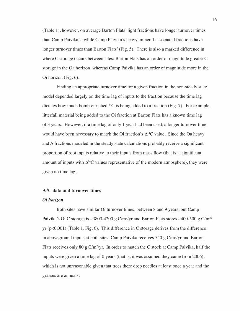
(‰)
Figure 1. Relationship between turnover time and ∆14C signature of soil organic matter (SOM; after Gaudinski et al., 2000). The peak in atmospheric 14C, or the bomb curve (solid line) in the 1960s allows determination of how fast a soil fraction is incorporating new material and hence its turnover time, because detectable amounts of 14C are incor-porated into SOM fixed after 1963. As the atmosphere became enriched with respect to 14C, SOM reservoirs began to incorporate detectable amounts of 14C: dotted curves show how the yearly 14C content of SOM would change each year given a turnover time (TT) of 10 versus 50 years, assuming that the fractions are homogenous, cycling at steady state, and have no time lag between fixation of C and incorporation into a fraction.
116º 51’00’’W) are located 42 km apart (Fig. 2). The two sites were chosen for
uniformity of tree species and soils and have a similar climate regime (Miller et al.,
1977). Camp Paivika is at 1600 m elevation and Barton Flats at 1946 m, which
influences their vegetation: both are characterized as mixed conifer forests, but Camp
Paivika is dominated by ponderosa pine, and Barton Flats has mixed ponderosa and
Jeffrey pine (Fenn and Dunn, 1989; Miller et al., 1989). Climate in the San Bernardino
Mountains is Mediterranean, characterized by warm, dry summers with winter snows as
the major source of moisture (Miller et al., 1977). Barton Flats and Camp Paivika have a
similar amount of yearly precipitation: averaged over 1980-1997, the two sites received
89.7 cm/yr and 98 cm/yr respectively (data for Barton Flats comes from nearby Camp
Osceola; see Fig. 2; Grulke and Balduman, 1999). Grulke and Balduman (1999) report
cooler temperatures and hence a shorter growing season at Barton Flats than at Camp
Paivika over 1993-1995. However, there is a large interannual variation in growing
season length at the sites, and the authors use few data points to measure this difference
and do not provide specific temperature data. In addition, it is likely that moisture affects
soil respiration and decomposition to an equal or greater degree than temperature (cf.
Trumbore, 1996; Trumbore and Harden, 1997; Hooper and Johnson, 1999; Davidson,
2000).
The soils at both sites are generally similar: they are formed on coarse-grained
weathered granitic parent material or colluvium derived from granites, and are well
drained with a low water holding capacity (Miller et al., 1977). Camp Paivika has
predominantly Shaver series soils (coarse loamy, mixed, superactive, mesic Humic
Dystroxerepts), and Barton Flats has Crouch and Cahto variant soils (coarse-loamy or
loamy-skeletal, mixed, superactive or active, mesic Humic Dystroxerepts; Arkley, 1981;
6
Hol
com
be C
r.
Mill
Cr.
San
ta A
na R
.
CP
BF
Silv
erw
ood
Lake
Lake
Gre
goryLa
keA
rrow
head
Big
Bea
r Lak
e
Bal
dwin
Lake
(dry
)
x S
an G
orgo
nio
Mtn
.
S
an G
orgo
nio
W
ilder
ness
0 1
2 3
4 5
Kilo
met
ers
Lake
Nat
iona
l For
est B
ound
ary
Figu
re 2
. Lo
catio
ns o
f the
sam
plin
g si
tes i
n th
e Sa
n B
erna
rdin
o M
ount
ains
(map
afte
r Fen
n an
d D
unn,
198
9).
Cam
p Pa
ivik
a (C
P) is
clo
ser t
o th
e po
lluta
nt so
urce
in L
os A
ngel
es th
an B
arto
n Fl
ats (
BF)
. So
me
site
dat
a fo
r Bar
ton
Flat
s is
extra
pola
ted
from
Cam
p O
sceo
la (C
O),
~3 k
m a
way
.
Key
Map
Los
Ang
eles
San
Ber
nard
ino
Mou
ntai
ns A
rea
CO
N
7
Soil Survey Staff, 1998).
Atmospheric pollutant deposition to the sites is primarily caused by fossil fuel
combustion in the Los Angeles Basin, which creates hydrocarbons and nitric oxide
(NO), and these products in turn generate tropospheric ozone (O3) (Miller et al., 1977;
Solomon et al., 1992; Fenn and Kiefer, 1999). Deposition decreases throughout the
mountains from west to east, along the direction of prevailing surface winds, due to rising
elevation and distance from the source of pollution (Fig. 3; Miller et al., 1977; Miller et
al., 1989; Takemoto et al., 2001). Nitrogen deposition levels show an especially dramatic
change because N species have a high depositional velocity, particularly nitric acid
(HNO3). Camp Paivika, in the western mountains, receives 35-45 kg N/ha/yr, whereas
Barton Flats, in the east, has N deposition of 5-9 kg/ha/yr (Bytnerowicz and Fenn, 1996;
Takemoto et al., 2001). N is deposited mostly as dry particulate nitrate (NO3-) and
HNO3, which adsorb onto foliage and later are mobilized in throughfall, though some
wet deposition of NO3- also occurs (Bytnerowicz and Fenn, 1996; Fenn and Kiefer, 1999;
Fenn et al., 2003; Grulke et al., 2005). Both sites also have higher than background
levels of ozone: Camp Paivika has 24-hour average O3 concentrations of ~0.09 ppm,
while Barton Flats has O3 concentrations of ~0.06 ppm (clean, background sites have O3
levels of ~0.015-0.04 ppm; Fenn and Dunn, 1989; Takemoto et al., 2001).
In order to study the effects of N on soil C cycling, it is necessary to discriminate
between the influences of N and O3. Many studies have focused on these pollutants’
impacts on the aboveground mixed conifer forest ecosystem and particularly ponderosa
pines because of their sensitivity to oxidant air pollution (Miller et al., 1983; Grulke
and Balduman, 1999). Elevated ozone levels have been demonstrated to cause foliar
injury and abscission as trees absorb ozone directly through stomates as well as lowering
root biomass, and greater N availability increases branchlet and bole growth, and also
contributes to lower root biomass (Miller et al., 1977; Miller et al., 1982; Gower et al.,
1996; Grulke et al., 1998; Grulke and Balduman, 1998; Miller and McBride, 1999;
8
San
Ber
nard
ino
Mou
ntai
ns
E
W
NS
CP
BF
Pollu
ted
air fl
ow
Figu
re 3
. To
pogr
aphy
and
dis
tanc
e fr
om L
os A
ngel
es c
reat
e th
e po
llutio
n gr
adie
nt o
bser
ved
in th
e Sa
n B
erna
rdin
o M
oun-
tain
s (fig
ure
afte
r Mill
er e
t al.,
197
7).
Atm
osph
eric
dep
ositi
on o
f N is
hig
her a
t Cam
p Pa
ivik
a (C
P), i
n th
e w
este
rn m
on-
tain
s, th
an fu
rther
to th
e ea
st a
t Bar
ton
Flat
s (B
F); C
amp
Paiv
ika
also
exp
rerie
nces
hig
her o
zone
pol
lutio
n.
9
Takemoto et al., 2001; Fenn et al., 2003).
The different effects of ozone on ponderosa pines at each site have been well-
documented. At Camp Paivika, ozone-injured ponderosa pines drop their needles
approximately once a year, but at Camp Osceola, in the area of Barton Flats, the trees
drop their needles once every 3 years; at background ozone levels ponderosa pines may
retain up to 6 years of needles (Grulke and Balduman, 1999; Takemoto et al., 2001).
Also, ponderosa pine root biomass at Camp Paivika is up to 6-14 times less than at Camp
Osceola (Grulke et al., 1998). Consequently, the influence of high ozone on soils at the
sites is probably indirect and limited to increasing litterfall inputs and lowering root
biomass. Little data is available concerning the direct impact of ozone on soils, so in
the absence of contradictory data this study assumes that all other differences in soil C
cycling observed between the sites are responses to N.
Field and laboratory work
The National Forest Service defined study plots at Camp Paivika and Barton Flats
in the 1970s, selecting for relative homogeneity of vegetation type and cover (Miller et
al., 1977, Fenn and Dunn, 1989). For this study, three ponderosa pines were chosen from
a plot at each site, and soil samples were collected 0.5 m from the northeast side of each
tree and homogenized. A 15 cm square portion of litter (Oi horizon) was cut out and a 5
cm diameter core was taken through the Oa horizon to approximately 10 cm depth in the
A horizon (Fig. 4).
Soil C storage (g C/m2) for each replicate soil horizon was calculated as bulk
density multiplied by g C/g soil (determined by CO2 purification on a vacuum line), and
the C storage within each separated soil fraction was extrapolated using a mass balance
scheme. C storage for each fraction is reported as the mean of the three replicates
analyzed, except that at Barton Flats the presence of a rock in the A horizon beneath one
tree prevented sampling, so only two replicates were used.
10
15 cm square of Oi horizon cut out
Sieved
5 cm diameter core takenthrough Oa and A horizons
Centrifuged with Na polytungstate solu-tion (2.0 g/cm3)
Ground Oi fraction
Oa coarse fraction
Oa fine material
> 1mm
Oa light fraction
A light fraction
Oa heavy fraction
A heavy fraction
}}
floatingmaterial
pellet
< 1mm
Figure 4. Schematic of the process of collecting soil samples and separating them into fractions; thick boxes indicate fractions that were analyzed for ∆14C. The resulting fractions have distinct physical and chemical characteristics that reflect their general stage of decomposition and turnover time. The Oi (litter) fraction contains undegraded pine needles, bark, and wood. The Oa coarse fraction is a mixture of Oi and Oa light material; the Oa and A light fractions are composed of labile organic matter that has been visibly decomposed. The Oa and A heavy fractions have humified or mineral-associated organic matter (Schulten and Leinweber, 1999; Gaudinski et al., 2000; Trumbore, 2000). Note that depths of soil horizons vary between sites.
Oi(litter)
Oa
A
Oa samples
A samples
11
The replicate samples from each horizon were homogenized for ∆14C analysis.
The Oi samples were ground, and soil samples from the Oa and A horizons were further
separated by size and density into fractions with different general turnover times, after
Gaudinski et al. (2000). The Oa samples were sieved to 1 mm, and the material smaller
than 1 mm was separated by density into light and heavy fractions by centrifuging with
a Na polytungstate solution (d = 2.0) (Fig. 4). ∆14C signatures for these fractions were
analyzed on an accelerator mass spectrometer (AMS) at the University of California,
Irvine. Sample targets were prepared using the zinc reduction technique with a Fe
catalyst (Vogel, 1992; Gaudinski et al., 2000). The AMS instrument used in this study
has a 2‰ precision, allowing age determination to within 1 year for samples made from
C fixed since the bomb curve peak in 1963.
Modeling
Determination of soil fraction turnover times from 14C values
A non-steady state accumulation model was used to calculate the turnover time
of the younger, lighter soil fractions (from the Oi and Oa horizons), which are more
dynamic and cycle on a faster timescale. For the A horizon and heavier Oa fraction, a
steady state model was used, given that these fractions cycle on longer timescales so
that their turnover time, age and residence time are approximately equal (Gaudinski et
al., 2000). Radiocarbon values were reported in the model as ∆14C, the amount of 14C in
‰ relative to the amount in an oxalic acid standard, OX1, in 1950, corrected for mass-
dependent fractionation to a δ13C value of -25‰ (Stuiver and Polach 1977):