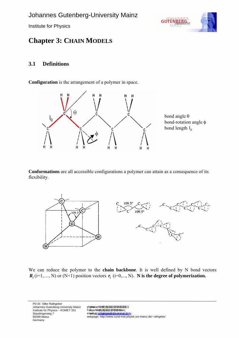
Chap3 Chain Models - userpages at the mean-square average (norm): 2 22 11 1 1 1 E 2 E NN N N N EE j...

Johannes Gutenberg-University Mainz Institute for Physics

PD Dr. Silke Rathgeber Johannes Gutenberg-University Mainz Institute for Physics – KOMET 331 Staudingerweg 7 55099 Mainz Germany

phone: +49 (0) 6131/ 392-3323 Fax: +49 (0) 6131/ 392-5441 email: [email protected]

phone: +49 (0) 6131/ 392-3323 Fax: +49 (0) 6131/ 392-5441 email: [email protected] webpage: http://www.cond-mat.physik.uni-mainz.de/~rathgebs/

Chapter 3: CHAIN MODELS 3.1 Definitions Configuration is the arrangement of a polymer in space.

bond angle θ bond-rotation angle φ bond length 0l

Conformations are all accessible configurations a polymer can attain as a consequence of its flexibility.

We can reduce the polymer to the chain backbone. It is well defined by N bond vectors

iR (i=1,…, N) or (N+1) position vectors ir (i=0,..., N). N is the degree of polymerization.



polar coordinates (θi,φi,|Ri|)

Degree of freedom (θ1, φ1, φ2) and the start vector r0 are undefined

⇒ global degree of freedom of rotation and translation ⇒ all others internal degree of freedom

Restrictions in the degree of freedom:

1. fixed bond length: covalent bond energy >> thermal energy 2. fixed bond angle: determined by electronic configuration of atoms building

the backbone 3. bond-rotation angle: relatively unrestricted

Comparison of single-bond in ethane and double-bond in ethene:

single-bond

double-bond



3.2 Characteristic quantities

End-to-End distance: 0

N

E N jj i

R r r R=

= − = ∑

Thermal movements: polymers adopt with time a large number of conformations, thus, thermal averages are considered. For an isotrope system: 0E ER R= = look at the mean-square average (norm):

2 2 2

1 1 1 1 12E E

N N N N N

E E j k j j kj k j j k j

R R R R R R R R R= = = = = +

= = = = +∑∑ ∑ ∑ ∑

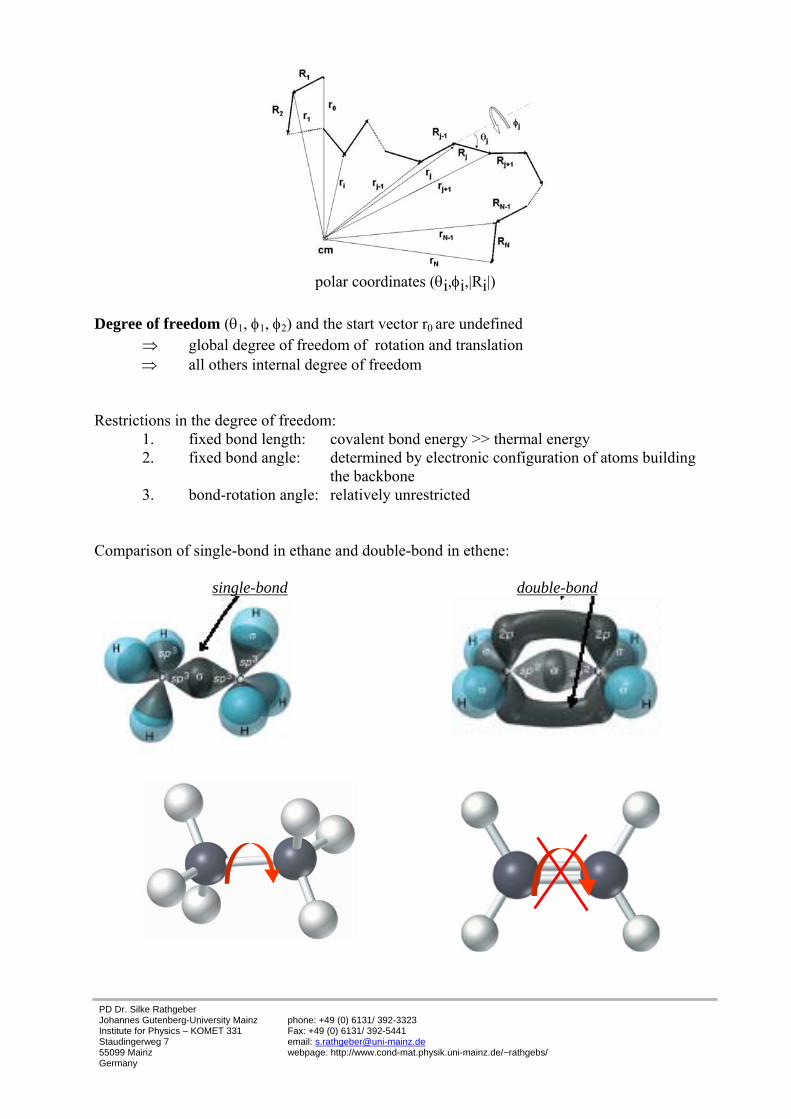
General definition of the radius of gyration gR : The radius of gyration of a mass about a given axis is a distance

gR from the axis at which an equivalent mass is thought of as a point mass. The moment of inertia of this point mass and original mass about the axis are the same. 2 2 2 2

, , ,g g x g y g zR R R R= + +

Radius of gyration gR is defined as the (average) of second moment (relative to the center of mass (rcm)) of the mass distribution:

( )2

2 02

0

N

j j cmj

g g N

jj

m r rR R

m

=

=

−= =

∑

∑

with 0

0

N

j jj

cm N

jj

m rr

m

=

=

=∑

∑

In case all masses are identical mj = m: ( )22

0

1 -1

N

g j cmj

R r rN =

=+ ∑ with

0

11

N

cm jj

r rN =

=+ ∑

With the help of the Lagrange Theorem: 2 2

21 1

1( 1)

N N

g iji j i

R rN = = +

=+ ∑ ∑ with ( )22

ij i jr r r= −

x

y z

Ri Ri+1

Rj

rj

ri

Ri-1

Rj+1 cm

rij



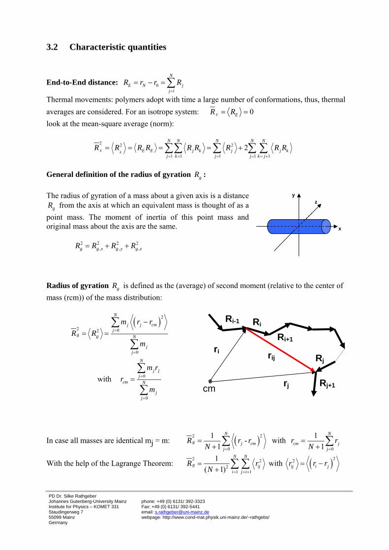
Characterization of the stiffness of a polymer: How is the orientientation of the end-to-end vector relative to the first bond vector? Projection HN of RE on the unit vector e1 (pointing in the direction of R1) HN is the sum of the projections of all bond vectors Rj on the direction of the first bond vector R1.

11 1

11 11 1 1

N NjE

N E jj j

R RR R RH e R RR R R= =

= = = =∑ ∑

The persistence length lP is defined as the thermal average in the limit of infinate long chain:

1

1 1

lim lim jP NN N j

R Rl H

R

∞

→∞ →∞=

≡ = ∑

3.3 Chain models For the calculation of the correlations between bond vectors j kR R and position vectors 2

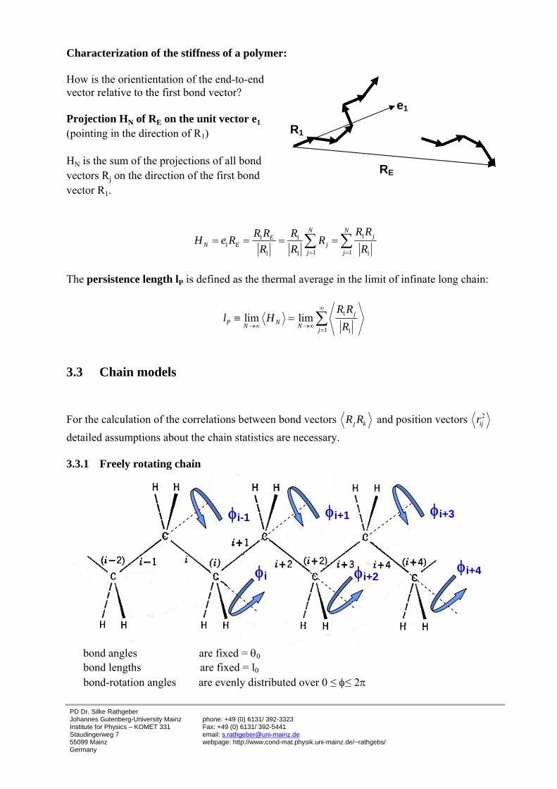
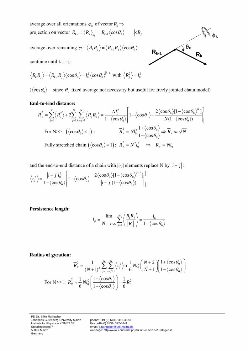
ijr detailed assumptions about the chain statistics are necessary. 3.3.1 Freely rotating chain

bond angles are fixed = θ0

bond lengths are fixed = l0

bond-rotation angles are evenly distributed over 0 ≤ φ≤ 2π

φi-1 φi+1 φi+3

φi φi+2 φi+4

RE

e1

R1



average over all orientations kϕ of vector kR ⇒

projection on vector 1kR − : -1 0cosk

k k jR R Rϕ

θ= ×

average over remaining iϕ : -1 0cosk j k jR R R R θ= continue until k-1=j:

-2-1 0 0 0cos cos k j

k j k jR R R R lθ θ= = with 2 20jR l=

( 0cosθ since 0θ fixed average not necessary but useful for freely jointed chain model) End-to-End distance:

22 0 02 00

1 1 1 0 0

2 cos [1 cos ]2 1 cos

1 cos (1 cos )E

NN N N

j j kj j k j

NlR R R RN

θ θθ

θ θ= = = +

⎡ ⎤−= + = + −⎢ ⎥

− −⎢ ⎥⎣ ⎦∑ ∑ ∑

For N>>1 ( )0cos 1θ < : 2 02

00

1 cos1 cosE ER Nl R N

θθ

+= ⇒ ∝

−

Fully stretched chain ( )0cos 1θ = : 2 2 2

0 0E ER N l R Nl= ⇒ = and the end-to-end distance of a chain with |i-j| elements replace N by i j− :

20 0 02

00 0

2 cos [1 cos ]1 cos

1 cos (1 cos )

i j

ij

i j lr

i jθ θ

θθ θ

−⎡ ⎤− −⎢ ⎥= + −

− − −⎢ ⎥⎣ ⎦

Persistence length:

1 0

1 1 0

lim1 cos

jP

j

R R llN R θ

∞

=

= =→ ∞ −∑

Radius of gyration:

2 02 2

021 1 0

1 cos1 1 2( 1) 6 1 1 cos

N N

g ijj i j

NR r NlN N

θθ= = +

⎛ ⎞++⎛ ⎞= ≈ ⎜ ⎟⎜ ⎟⎜ ⎟+ + −⎝ ⎠⎝ ⎠∑ ∑

For N>>1: 2 02 2

00

1 cos1 16 1 cos 6

g ER Nl Rθθ

⎛ ⎞+≈ =⎜ ⎟⎜ ⎟−⎝ ⎠

φk

Rk Rk-1 θ0



3.3.2 Freely jointed chain

bond angles are evenly distributed over 0 ≤ θ ≤ 2π bond lengths are fixed 0l=

bond-rotation angles are evenly distributed over 0 ≤ φ ≤ 2π ⇒ Special case of a freely rotating chain with cos 0θ =

End-to-End distance:

22 0 0 20

0 00 0

2 cos [1 cos ]1 cos

1 cos (1 cos )E

NNlR Nl

Nθ θ

θθ θ

⎡ ⎤−= + − =⎢ ⎥

− −⎢ ⎥⎣ ⎦

and for the end-to-end distance of a chain with |i-j| elementsreplace N by i j−

2 20ijr i j l= −

Persistence length:

00

01 cosPll l

θ= =

−

Radius of gyration:

2 2 2

0 02

1 1 ( 1)( 1)( 1) 6

N

gi j

N NR i j l lN N<

− += − =

+ ∑

For N>>1: 2 22

01 16 6

g ER Nl R≈ =

The end-to-end distance

2 20ER Nl= is in analogy to a 3-dimensional random walk!

θi-1 θi+1 θi+3

θi θi+2 θi+4 θi-2



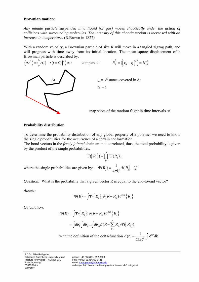
Brownian motion: Any minute particle suspended in a liquid (or gas) moves chaotically under the action of collisions with surrounding molecules. The intensity of this chaotic motion is increased with an increase in temperature. (R.Brown in 1827) With a random velocity, a Brownian particle of size R will move in a tangled zigzag path, and will progress with time away from its initial location. The mean-square displacement of a Brownian particle is described by:

[ ]22 ( ) ( 0)r r t r t tΔ = − = ∝ compare to [ ]2 2 20 0E NR r r Nl= − =

0 distance covered in t l

N t

≡ Δ

≡

snap shots of the random flight in time intervals Δt

Probability distribution To determine the probability distribution of any global property of a polymer we need to know the single probabilities for the occurrence of a certain conformation. The bond vectors in the freely jointed chain are not correlated, thus, the total probability is given by the product of the single probabilities.

{ }1

( ) ( )N

j jj

R R=

Ψ = Ψ∏ ,

where the single probabilities are given by: 020

1( ) ( )4j jR R l

lδ

πΨ = −

Question: What is the probability that a given vector R is equal to the end-to-end vector? Ansatz:

{ } { }3( ) ( ) ( ) Nj E jR R R R d RδΦ = Ψ −∫

Calculation:

{ } { }

{ }

3

1 21

( ) ( ) ( )

... ( ) ( )

Nj E j

N

N j jj

R R R R d R

dR dR dR R R R

δ

δ=

Φ = Ψ −

= − Ψ

∫

∑∫ ∫ ∫

with the definition of the delta-function 3

1( )(2 )

ikrr e dkδπ

= ∫

Δt



{ }

0

0

1 231

131

3

sin( )

1( ) ... exp[ ( )] ( )(2 )

1 exp( ) ... exp( ) ( )(2 )

1 exp( ) exp( ) ( ) (2 )

N

N j jj

N

N j jj

N

klkl

R dk dR dR dR ik R R R

dk ikR dR dR ikR R

dk ikR dR ikR R

π

π

π

=

=

=

Φ = − Ψ

= − Ψ

⎡ ⎤= − Ψ⎣ ⎦

∑∫ ∫ ∫ ∫

∏∫ ∫ ∫

∫ ∫14444244443

up to here: same for the gaussian chain with polar coordinates ( )i i rθ φ

0

03

0

small apart for small kl

2 20 0 0

0

sin( )1( ) exp( )(2 )

approximation for large N:

sin( ) ( ) ( )replace 1 exp6 6

N

N N

klR dk ikRkl

kl kl N klkl

π⎡ ⎤

Φ = ⎢ ⎥⎣ ⎦

⎡ ⎤ ⎛ ⎞ ⎛ ⎞≈ − ≈ −⎜ ⎟ ⎜ ⎟⎢ ⎥

⎝ ⎠ ⎝ ⎠⎣ ⎦

∫14243

20

3

2 2 2 2

322

2 20 0

vanishs also for large N!

( )1( ) exp( ) exp(2 ) 6

with and k

3 3( ) exp22 2

x x y y z z x y z

N klR dk ikR

kR k R k R k R k k k

RRNl Nl

π

π

⎛ ⎞Φ = −⎜ ⎟

⎝ ⎠= + + = + +

⎛ ⎞ ⎛ ⎞Φ = −⎜ ⎟ ⎜ ⎟

⎝ ⎠ ⎝ ⎠

∫

Result:

3/ 2 2

2 20 0

3 3( ) exp2 2 2

RRNl Nlπ

⎛ ⎞ ⎛ ⎞Φ = −⎜ ⎟ ⎜ ⎟

⎝ ⎠ ⎝ ⎠

Gaussian distribution Effective bond length In case only local correlations are effective, so that

{ } 1 21

( ) ( , , ,..., ) withc

c

N j

j j j j j j cj

R R R R R j N−

+ + +=

Ψ = Ψ <<∏

the real chain can always be described by a freely jointed chain with larger effective bond length,

so that the relations 2 2ER Nl= and 2 21

6g ER R= for large N still hold.



Characteristic ratio

2 2

02 20 0

lim E

N

R lC l C lNl l∞ ∞→∞

= = ⇒ =

e.g. freely rotating chain 0

0

1 cos1 cos

Cθθ∞

+=

−

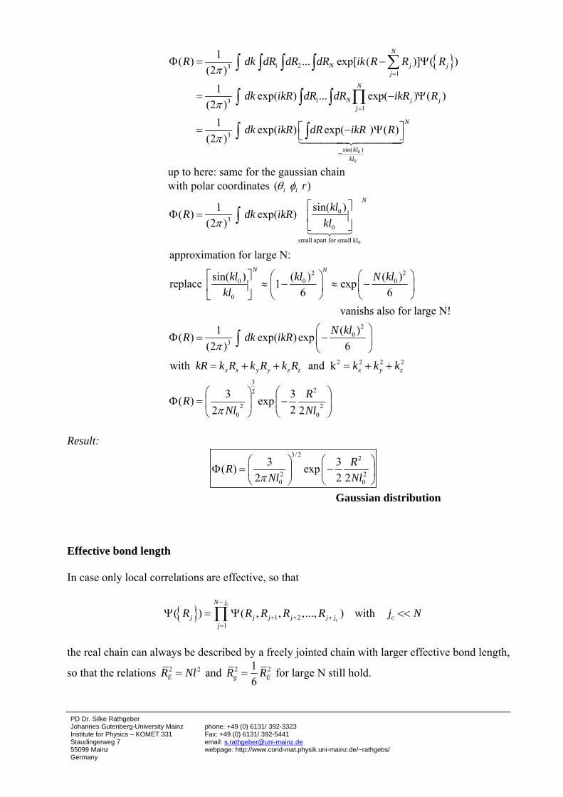
Kuhn segment is defined by a transformation of the real chain onto a freely jointed chain under preservation of the end-to-end distance 2

ER and the maximal possible end-to-end distance of the fully stretched chain ,maxER

2 2

,max and E k k E k kR N l R N l= = ⇒ the number and the length of the (effective) segments are rescaled.

22

,max2

,max

and EEk k

E E

RRl NR R

= =

Segments of length lk are the smallest units being statistically uncorrelated. The Kuhn segment is like the persistence length a measure of the chain stiffness. e.g. freely rotating chain

0 70.53θ = ° (tetrahedron angle)

( )

02 20

0

0,max 0 0 0

20

0 0,max 0

2,max 0

2

1 cos1 cos

1 coscos 2

2

2(1 cos ) 2.451 cos

1 cos0.33

2

E

E

Ek

E

Ek

E

R Nl

R Nl Nl

lRl lR

RN N N

R

θθ

θθ

θθ

θ

+=

−

+= =

⇒ = = + ≈ ×−

−= = ≈ ×

θ0

θ0/2

lk, Nk

l0, N

l0



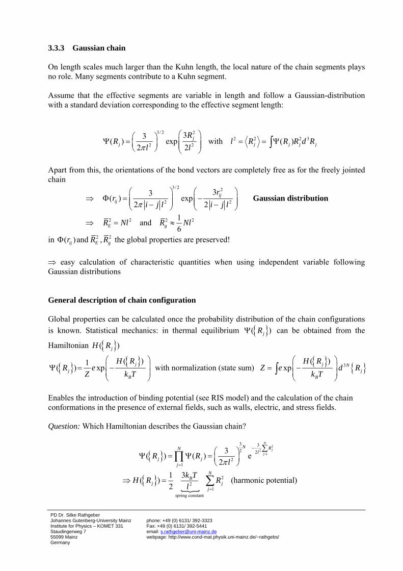
3.3.3 Gaussian chain On length scales much larger than the Kuhn length, the local nature of the chain segments plays no role. Many segments contribute to a Kuhn segment. Assume that the effective segments are variable in length and follow a Gaussian-distribution with a standard deviation corresponding to the effective segment length:

3/ 2 2

2 2 2 32 2

33( ) exp with ( )2 2

jj j j j j

RR l R R R d R

l lπ⎛ ⎞⎛ ⎞Ψ = = = Ψ⎜ ⎟⎜ ⎟ ⎜ ⎟⎝ ⎠ ⎝ ⎠

∫

Apart from this, the orientations of the bond vectors are completely free as for the freely jointed chain

3/ 2 2

2 2

33( ) exp2 2

ijij

rr

i j l i j lπ⎛ ⎞⎛ ⎞

⇒ Φ = −⎜ ⎟⎜ ⎟⎜ ⎟ ⎜ ⎟− −⎝ ⎠ ⎝ ⎠ Gaussian distribution

2 2 2 21and6E gR Nl R Nl⇒ = ≈

in 2 2( ) and ,ij E gr R RΦ the global properties are preserved! ⇒ easy calculation of characteristic quantities when using independent variable following Gaussian distributions General description of chain configuration Global properties can be calculated once the probability distribution of the chain configurations is known. Statistical mechanics: in thermal equilibrium { }( )jRΨ can be obtained from the

Hamiltonian { }( )jH R

{ } { } { } { }3( ) ( )1( ) xp with normalization (state sum) xpj j N

j jB B

H R H RR e Z e d R

Z k T k T

⎛ ⎞ ⎛ ⎞⎜ ⎟ ⎜ ⎟Ψ = − = −⎜ ⎟ ⎜ ⎟⎝ ⎠ ⎝ ⎠

∫ Enables the introduction of binding potential (see RIS model) and the calculation of the chain conformations in the presence of external fields, such as walls, electric, and stress fields. Question: Which Hamiltonian describes the Gaussian chain?

{ }2

21

3 32 2

21

3( ) ( ) e2

N

jj

N RNl

j jj

R Rlπ

=

−

=

∑⎛ ⎞Ψ = Ψ = ⎜ ⎟⎝ ⎠

∏

{ }{

22

1spring constant

31( ) (harmonic potential)2

NB

j jj

k TH R Rl =

⇒ = ∑



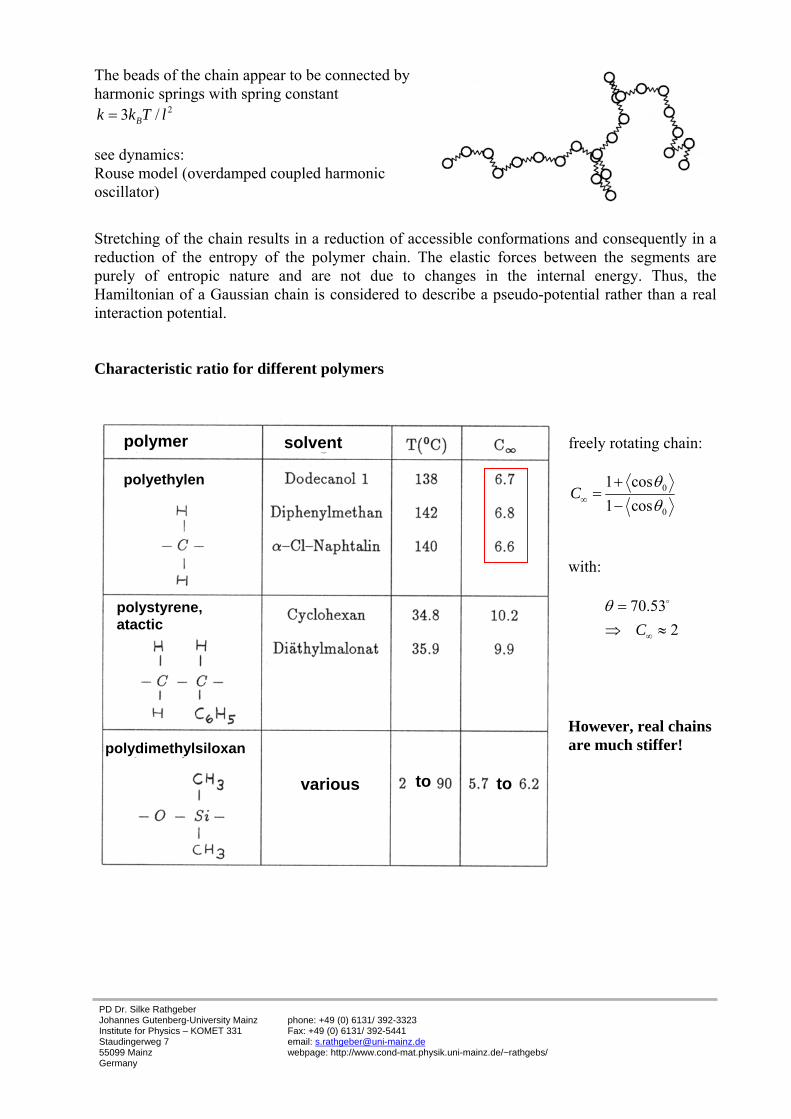
The beads of the chain appear to be connected by harmonic springs with spring constant

23 /Bk k T l= see dynamics: Rouse model (overdamped coupled harmonic oscillator)

Stretching of the chain results in a reduction of accessible conformations and consequently in a reduction of the entropy of the polymer chain. The elastic forces between the segments are purely of entropic nature and are not due to changes in the internal energy. Thus, the Hamiltonian of a Gaussian chain is considered to describe a pseudo-potential rather than a real interaction potential. Characteristic ratio for different polymers

freely rotating chain:

0

0

1 cos1 cos

Cθθ∞

+=

−

with:

70.532C

θ

∞

=⇒ ≈

o

However, real chains are much stiffer!

polymer solvent

various to to

polyethylen

polystyrene, atactic

polydimethylsiloxan



RIS Bond rotational potentials The picture of unrestricted freedom of bond-rotation angles is oversimplified. Finite extension of atoms and side groups lead to "long-ranged" (excluded volume interactions, prohibition of chain intersections) as well as "short-ranged interactions". Due to sterical hindrance not all bond rotation angles have the same probability. Some bond- rotation angles are compared to other energetically favorable. Bond rotational potentials { } 1 1 1( ) ( ,..., , , ,..., )i i i i NH H H − += Φ = Φ Φ Φ Φ Φ

{ } { } { } { }( ) ( )1( ) xp with normalization xpi i Ni i

B B

H He Z e d

Z k T k T⎛ ⎞ ⎛ ⎞Φ Φ

Ψ Φ = − = − Φ⎜ ⎟ ⎜ ⎟⎝ ⎠ ⎝ ⎠

∫

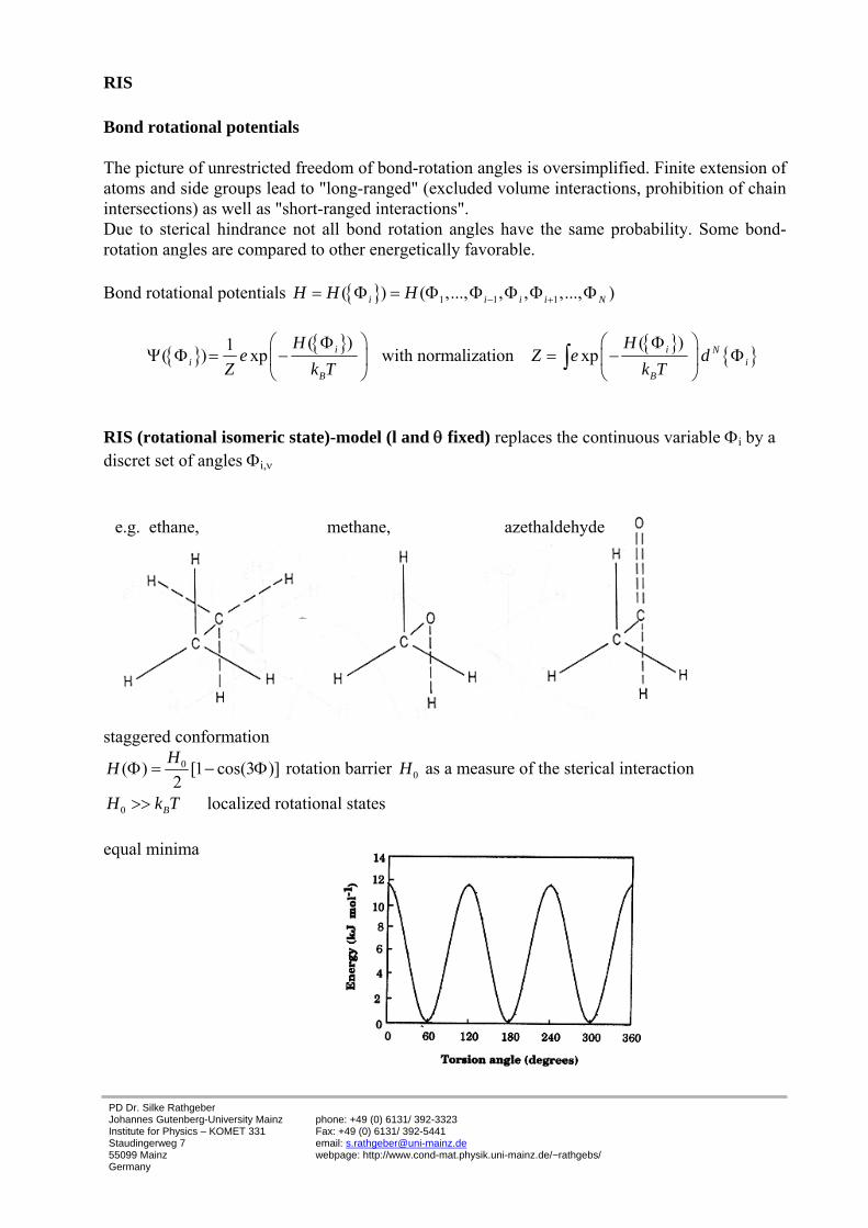
RIS (rotational isomeric state)-model (l and θ fixed) replaces the continuous variable Φi by a discret set of angles Φi,ν

staggered conformation

0( ) [1 cos(3 )]2

HH Φ = − Φ rotation barrier 0H as a measure of the sterical interaction

0 BH k T>> localized rotational states equal minima

e.g. ethane, methane, azethaldehyde



Barrier height thermal energy at 300K ≈ 0.6 kcal/mole (1 Joule = 2.390 ×10−4 kcal)

e.g. n-butane

minima are not equal 180 : 0o

t ttrans HΦ = = 60 : 0o

g ggauche H+ + +Φ = >

300 : 0og g ggauche H H− − − +Φ = = >

with the probability 1( ) exp mit Z expB B

H HZ k T k T

ν νν

ν

⎛ ⎞ ⎛ ⎞Ψ Φ = − = −⎜ ⎟ ⎜ ⎟

⎝ ⎠ ⎝ ⎠∑

ethane

methane

azethaldehyde propylene

dimethylether

butane

methanethiol

trans gauche

methylphosphine



Independent bond rotation potentials

{ }1

( ) ( )N

i i ii

H H=

Φ = Φ∑2 for freely rotating chain

1 cos 1 cos1 cos 1 cos

Cφ θφ θ∞

≈

+ +⇒ = ×

− −14243

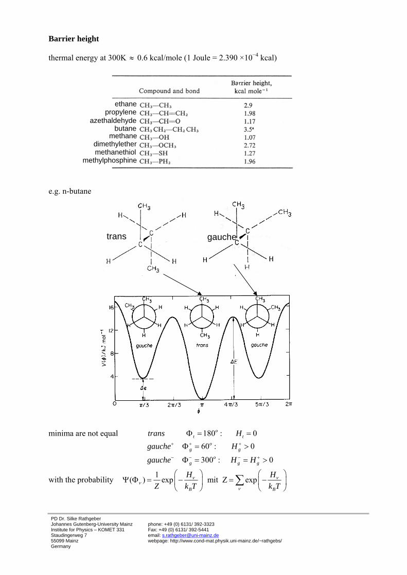
e.g. polyethylene @ 140 CT = o : 0.5 kcal/mole; 120 ; 70.53g gH θ± ±= Φ ≈ ± =o o

0; 0t tH = Φ ≈ o

1cos ; exp 0.543

1cos exp cos =1- - =1- with Z= exp =1+ =1+22 2

B

B B

Hk T

H HZ k T k T

ν

ν νν

ν ν

θ σ

σ σ σ σ σ σ

⎛ ⎞= = − =⎜ ⎟

⎝ ⎠

⎛ ⎞ ⎛ ⎞Φ = − Φ − +⎜ ⎟ ⎜ ⎟

⎝ ⎠ ⎝ ⎠∑ ∑

1cos 0.22 3.141 2

Cσσ ∞

−⇒ Φ = ≈ ⇒ ≈

+

still much smaller than experimental value: exp 6.7C∞ ≈ => real chains are much stiffer! Bond rotation potentials are not independent! rotation around single bond:

rotation around two bonds:

n-butane

trans

gauche

n-pentane

CH3 CH3

energetically unfavourable



Interdependent rotation potentials of adjascent bonds { }( ) ( )12

,N

i i ii

H H −=

Φ = Φ Φ∑

Ab-initio calculations: microscopic, quantum mechanic problem. Semi-empirical methods: "molecular force field" calculations based on Newton's mechanics and electrostatics. Atoms are replaced by beads and bonds by springs. Goal: find 3-dim structure with minimal energy. e.g. polyethylene:

3.3.4 Worm-like chain (Kratky-Porod model) Examples

contour length L = maximum end-to-end distance of a polymer

Pl L>>Pl L≈

Pl L<<



bond lengths are fixed = l0

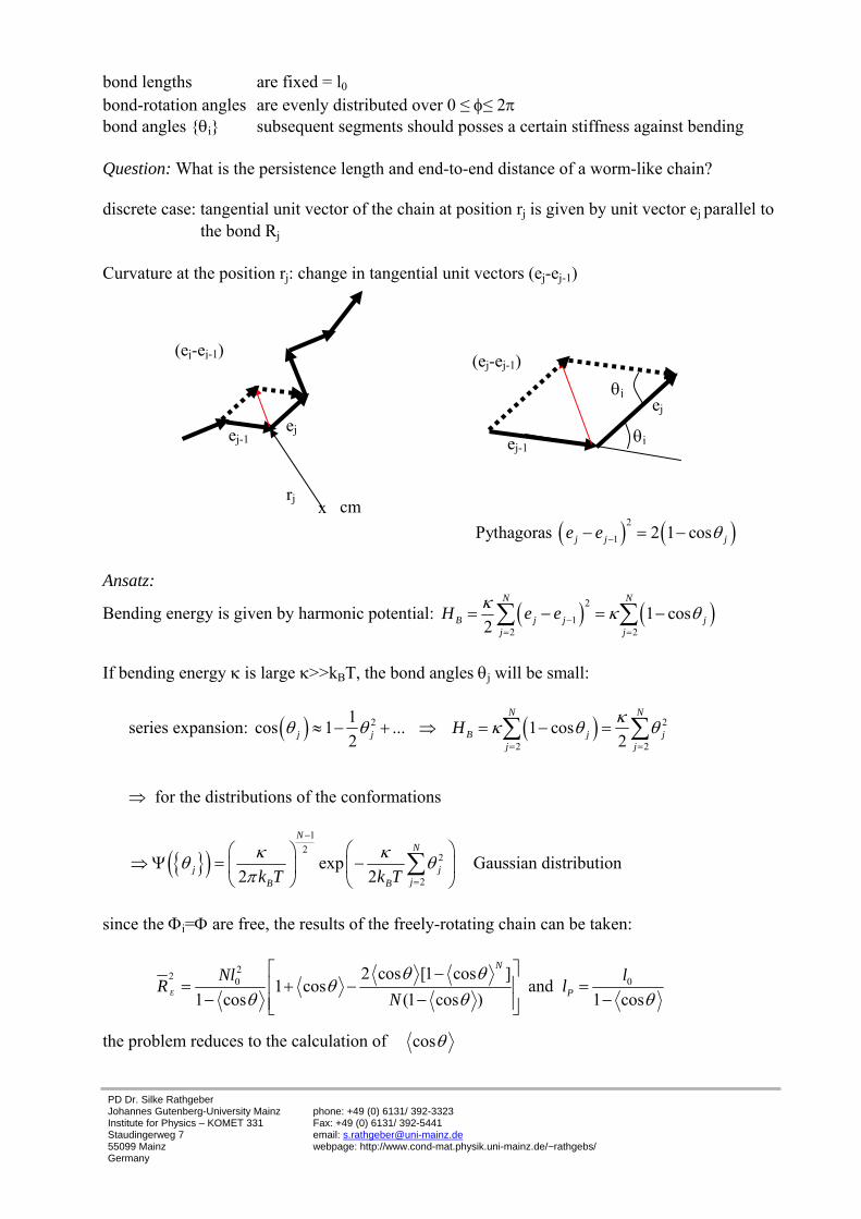
bond-rotation angles are evenly distributed over 0 ≤ φ≤ 2π bond angles {θi} subsequent segments should posses a certain stiffness against bending Question: What is the persistence length and end-to-end distance of a worm-like chain? discrete case: tangential unit vector of the chain at position rj is given by unit vector ej parallel to

the bond Rj Curvature at the position rj: change in tangential unit vectors (ej-ej-1)

( ) ( )2

1Pythagoras 2 1 cosj j je e θ−− = − Ansatz:

Bending energy is given by harmonic potential: ( ) ( )2

12 2

1 cos2

N N

B j j jj j

H e eκ κ θ−= =

= − = −∑ ∑

If bending energy κ is large κ>>kBT, the bond angles θj will be small:

series expansion: ( ) ( )2 2

2 2

1cos 1 ... 1 cos2 2

N N

j j B j jj j

H κθ θ κ θ θ= =

≈ − + ⇒ = − =∑ ∑

⇒ for the distributions of the conformations

{ }( )1

22

2exp

2 2

NN

j jjB Bk T k T

κ κθ θπ

−

=

⎛ ⎞⎛ ⎞⇒ Ψ = −⎜ ⎟⎜ ⎟

⎝ ⎠ ⎝ ⎠∑ Gaussian distribution

since the Φi=Φ are free, the results of the freely-rotating chain can be taken:

22 0 02 cos [1 cos ]

1 cos and 1 cos (1 cos ) 1 cosE

N

PNl lR l

Nθ θ

θθ θ θ

⎡ ⎤−= + − =⎢ ⎥

− − −⎢ ⎥⎣ ⎦

the problem reduces to the calculation of cosθ

θj

θj

ej-1

ej

(ej-ej-1)

ej ej-1

(ej-ej-1)

rj x cm



{ }( ) { }1cos cos exp2

N Bi i i

k Tdθ θ θ θκ

− ⎛ ⎞= Ψ = −⎜ ⎟⎝ ⎠∫

00

2 for 1 exp

2

P BB B

ll l k Tk T k T

κ κ

κ

= ≈ >>⎛ ⎞− −⎜ ⎟⎝ ⎠

22 02exp [1 exp ]

2 21 exp21 exp (1 exp )

2 2

E

NB B

B

B B

k T k TNl k TR

k T k TN

κ κκ

κ κ

⎡ ⎤⎛ ⎞ ⎛ ⎞− − −⎜ ⎟ ⎜ ⎟⎢ ⎥⎛ ⎞ ⎝ ⎠ ⎝ ⎠⎢ ⎥= + − −⎜ ⎟⎛ ⎞ ⎛ ⎞⎝ ⎠⎢ ⎥− − − −⎜ ⎟ ⎜ ⎟⎢ ⎥⎝ ⎠ ⎝ ⎠⎣ ⎦

2ER expressed as a function of lP, l0 and 0L Nl=

( )2 00 02 2 ( ) 1 1E

N

P P PP

lR L l l l l ll

⎡ ⎤⎛ ⎞⎢ ⎥= − − − − −⎜ ⎟⎢ ⎥⎝ ⎠⎣ ⎦

for large N replace 0 01 expN

P P

l Nll l

⎛ ⎞ ⎛ ⎞− ≈ −⎜ ⎟ ⎜ ⎟

⎝ ⎠ ⎝ ⎠

( )2

0 02 2 ( ) 1 expE P P PP

LR L l l l l ll

⎡ ⎤⎛ ⎞⇒ = − − − − −⎢ ⎥⎜ ⎟

⎝ ⎠⎣ ⎦

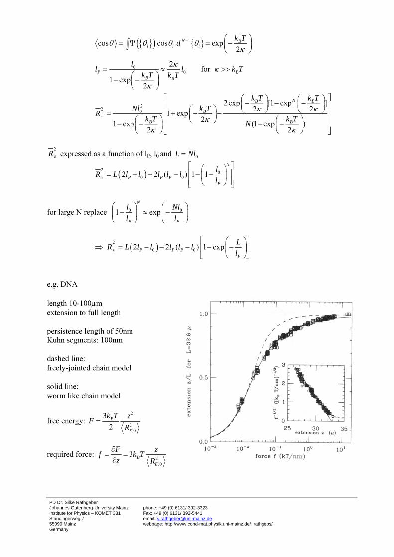
e.g. DNA length 10-100μm extension to full length persistence length of 50nm Kuhn segments: 100nm dashed line: freely-jointed chain model solid line: worm like chain model

free energy: 2

2,0

32B

E

k T zFR

=

required force: 2

,0

3 BE

F zf k Tz R

∂= =

∂



3.4 Polymer solutions Up to now we neglected any "long-ranged" interactions involving chain segments well separated along the chain. Backfolding of the chain due to the high chain flexibility has the consequence that distant chain segments can become very close to each other. However, chain segments have finite extension and interpenetration of volume occupied by other segments is forbidden This effect is called excluded volume interaction with the consequence that the extension of the coil will be larger than that of an "ideal chain" without excluded volume interactions. Excluded volume interactions lead to swelling! In the melt the interaction between segments in one chain is equal to the interaction with neighboring chains. The segment concentration is high and a segment of one chain is in the average surrounded by many segments belonging to other chains

⇒ excluded volume interaction is screened!

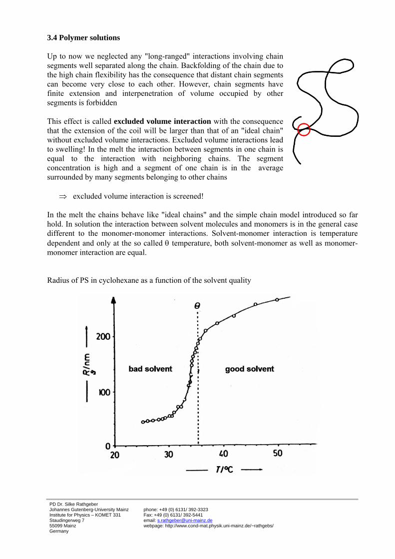
In the melt the chains behave like "ideal chains" and the simple chain model introduced so far hold. In solution the interaction between solvent molecules and monomers is in the general case different to the monomer-monomer interactions. Solvent-monomer interaction is temperature dependent and only at the so called θ temperature, both solvent-monomer as well as monomer-monomer interaction are equal. Radius of PS in cyclohexane as a function of the solvent quality



Gaussian chain with excluded volume interaction Also excluded volume interaction is short-ranged (of local nature), it effects distant segments on the chain. The concrete nature might be complicated but unimportant on larger scales.

,0 0

1( ) in total ( )2ij excl B i j excl B i j

j iH k T r r H k T r rυ δ υ δ

= =

= − ⇒ = −∑∑

Here υ represents the excluded volume and δ the delta function. For a Gaussian chain with excluded volume interactions we obtain for the probability distribution:

{ }( ) { }( ) { }( ) ( ) ( )2

12

interaction between interaction between neighbouring segments distant segments

3exp exp2 2

G j excl jj j j j i

j i jB

H r H rr r r r r

k T lυ δ−

⎛ ⎞⎜ ⎟⎡ ⎤+ ⎜ ⎟⎢ ⎥Ψ ∝ − ∝ − − − −⎜ ⎟⎢ ⎥ ⎜ ⎟⎣ ⎦⎜ ⎟⎝ ⎠

∑ ∑∑144424443144424443

Rigorous solution of the problem not possible! Flory theory Question: What is the end-to-end distance 2

ER of a chain with excluded volume interaction? We start with a chain with radius R and N segments for a particle with arbitrary dimension d. Excluded volume interaction is proportional to the number of pair contacts 2c∝ where c is the concentration.

We obtain for the internal chain concentration: int d

NcR

=

Energy for one pair contact 2( ) dexcl Bf k T T c lυ≈ (υ excluded volume has dimension of a d-

dimensional volume) In mean field theory the specific correlation between monomers (local heterogenities) are neglected ⇒ assumption: 22 2

intc c c→ ∝ Total free energy by integration over total volume dR :

22int( ) ( )

dd ddexcl B B

N lF k T T R c l k T T Rυ υ≈ =

Entropy contributes as elastic term relative to ideal chain:



( )2 2

2 2el B BE

R RF k T k TR Nl

≈ =

Total free energy: ( )

22

2

( ) del B

dB

F k TRT N lk T R Nl

υ≈ +

Minimum for: 2 2 3 3/( 2)d d dR l N R lN N lν+ + +∝ ⇔ ∝ ∝ => Flory exponent 3/( 2)dν = + ν= 3/5 for d=3

3/4 d=2 1 d=1 Mean field approach (MFT) The main idea of MFT is to replace all interactions to any one body with an average or effective interaction. This reduces any multi-body problem into an effective one-body problem. A many-body system with interactions is generally very difficult to solve exactly, except for extremely simple cases (Gaussian field theory, 1D Ising model.) The great difficulty (e.g. when computing the partition function of the system) is the treatment of combinatorics generated by the interaction terms in the Hamiltonian when summing over all states. The goal of mean field theory (MFT, also known as self-consistent field theory) is to resolve these combinatorial problems. The main idea of MFT is to replace all interactions to any one body with an average or effective interaction. This reduces any multi-body problem into an effective one-body problem. The ease of solving MFT problems means that some insight into the behavior of the system can be obtained at a relatively low cost. In field theory, the Hamiltonian may be expanded in terms of the magnitude of fluctuations around the mean of the field. In this context, MFT can be viewed as the "zeroth-order" expansion of the Hamiltonian in fluctuations. Physically, this means a MFT system has no fluctuations, but this coincides with the idea that one is replacing all interactions with a "mean field". Quite often, in the formalism of fluctuations, MFT provides a convenient launch-point to studying first or second order fluctuations. In general, dimensionality plays a strong role in determining whether a mean-field approach will work for any particular problem. In MFT, many interactions are replaced by one effective interaction. Then it naturally follows that if the field or particle exhibits many interactions in the original system, MFT will be more accurate for such a system. This is true in cases of high dimensionality, or when the Hamiltonian includes long-range forces. The Ginzburg criterion is the formal expression of how fluctuations render MFT a poor approximation, depending upon the number of spatial dimensions in the system of interest. While MFT arose primarily in the field of Statistical Mechanics, it has more recently been applied elsewhere, for example for doing Inference in Graphical Models theory in artificial intelligence.



3.6 Self-similarity and fractal dimension of polymers

Looking at ensemble averages the relation between n and 2R stays the same for any

subsection of the chain with n segments as long as N>>n>>1. The relation between mass and volume defines the fractal dimension fD fDmass volume R∝ ∝

( )2fD

n R∝

solid body 3-dim body 3fD = 2-dim 2fD = 1-dim 1fD = Polymers: ideal chain 2 2 2fR Nl D= ⇒ = with excluded volume interaction 3-dim 3/5 5 3fR N l D∝ ⇒ =

2-dim 3/ 4 4 3fR N l D∝ ⇒ = 1-dim 1fR Nl D∝ ⇒ =



3.7 Summary characteristic quantities: Rg, RE, lP describe dimension & stiffness in an ensemble of polymers. All orientations have same probabilty in isotropic system ⇒ <Rg>, <RE>=0

⇒ look at the norms (mean square values) <Rg2>, <RE2> ⇒ geometrical considerations lead to <Rg2>, <RE2> and lP in terms of <RiRj> and <(ri-rj)2> ⇒ for the calculation of <RiRj> and <(ri-rj)2> assumptions about the chain statistics are

necessary / probability to find a certain l,φ, θ Determination of the probability distribution of any global property requires the knowledge of the single probabilities for the occurance of a certain conformation. ⇒ chain models

1. freely rotating chain l, θ = fixed & φ totaly free 2. freely jointed chain l = fixed & θ, φ = totaly free

⇒ <RE2>=Nl2 and <Rg2>=Nl2 and its analogy to random walk (chaotic motion) of Brownian particles.

total probability { }1

( ) ( )N

j jj

R R=

Ψ = Ψ∏

only local correlations { } 1 21

( ) ( , , ,..., )c

c

N j

j j j j j j cj

R R R R R mit j N−

+ + +=

Ψ = Ψ <<∏

⇒.real chain can be transformed onto freely jointed chain with different segment length (and) segment number under preservation of global properties. ⇒ this led us to definition of characteristic ratio & Kuhn length (measure of chain stiffness). one effective segment is made up by several real bonds ⇒

3. Gaussian chain θ, φ = totaly free effective segments are variable in length and follow a Gauss-distribution with a standard deviation corresponding to the effective segment length

3/ 2 2

2 2 2 32 2

33( ) exp with ( )2 2

jj j j j j

RR l R R R d R

l lπ⎛ ⎞⎛ ⎞Ψ = = = Ψ⎜ ⎟⎜ ⎟ ⎜ ⎟⎝ ⎠ ⎝ ⎠

∫

{ }32 2

2 211

3 3( ) ( ) exp2 2

NN N

j j jjj

R R Rl lπ ==

⎛ ⎞⎛ ⎞Ψ = Ψ = −⎜ ⎟⎜ ⎟⎝ ⎠ ⎝ ⎠

∑∏



global properties are preserved! statistical mechanics: { }( )jRΨ can be obtained from the Hamiltonian { }( )jH R

{ } { } { } { }3( ) ( )1( ) xp normalization xpj j N

j jB B

H R H RR e Z e d R

Z k T k T

⎛ ⎞ ⎛ ⎞⎜ ⎟ ⎜ ⎟Ψ = − = −⎜ ⎟ ⎜ ⎟⎝ ⎠ ⎝ ⎠

∫

which Hamiltonian describes the Gaussian chain?

⇒ harmonic potential { }{

22

1spring constant

31( )2

NB

j jj

k TH R Rl =

= ∑

chain appears to be made up by beads connected by harmonic springs ⇒ Rouse model (overdamped coupled harmonic oscillator)

4. RIS (Rotational Isomeric State model) l, θ = fixed replaces the continuous variable Φi by a discret set of angles Φi,ν where adjacent bonds are interdependent.

5. worm-like chain model l = fixed & φ = totally free

restrictions to θ: subsequent segments posses a certain stiffness against bending. so far only local interactions involving close-by bonds excluded volume interactions

• interpenetration of volume occupied by other segments is forbidden. • short-ranged but can involve distant chain segments on one chain. • rigorous calculation of global properties is not possible.

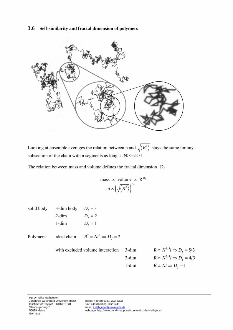
⇒ Mean-Field Theory of Flory for the free energy one obtains for the extension of a polymer chain under excluded volume interactions R N lν∝ with the Flory-Huggins exponent ν = 3/5 for d=3 3/4 d=2 1 d=1 compare to ideal chain 1/ 2R N l∝ Looking at ensemble averages polymers are self-similar structures i.e. fractal objects as long as subsections of the chains are considered which comprise much more than only one and much less than N segments.



Literature 1. U.W. Gedde, “ Polymer Physics”, Chapman & Hall, London, 1995.

2. G. Strobl, “ The Physics of Polymers”, Springer-Verlag, Berlin, 1996.

3. H.G. Elias, “ Makromoleküle Band 1: Chemische Struktur und Synthesen”, Wiley-VCH,

Weinheim, 1999.

4. S. Hoffmann, “Conformations of Polymer Chains”, Lecture Manuscripts of the 33th IFF

Winter School on “Soft Matter – Complex Materials on Mesoscopic Scales”, 2002.

5. H. Frielinghaus, “ Flexible Polymers”, Lecture Manuscripts of the 35th IFF Winter School

on “ Physics meets Biology – From Soft Matter to Cell Biology”, 2004.

6. K. Sturm, “Konformationen”, Lecture Manuscripts of the 22th IFF Winter School on

“Physik der Polymere”, 1991.

Date post:	12-May-2018
Category:	Documents
Upload:	lamkiet
View:	216 times
Download:	3 times

Chap3 Chain Models - userpages at the mean-square average (norm): 2 22 11 1 1 1 E 2 E NN N N N EE j...

Documents