29
1 Chapter 10 Determining how costs behave
| Date post: | 31-Dec-2015 |
| Category: |
Documents |
| Upload: | cairo-walker |
| View: | 45 times |
| Download: | 6 times |
1
Chapter 10
Determining how costs behave
2
Introduction
How do managers know what price to charge, whether to make or buy, or other questions related to costs.
They need to have an understanding of how costs change in relation to various factors.
This chapter will focus on how to determine cost behavior.
3
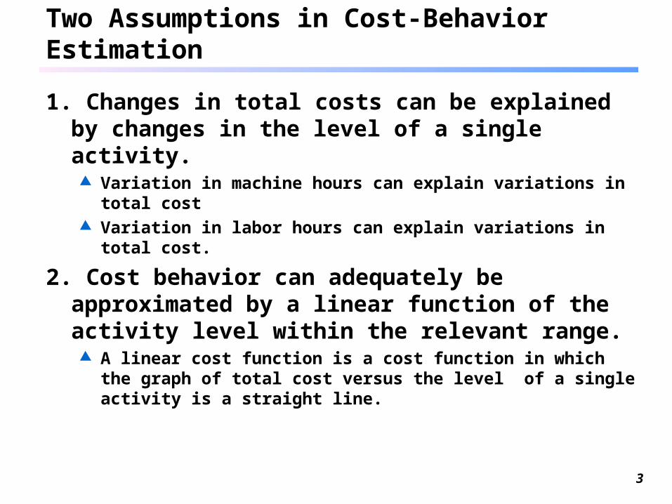
Two Assumptions in Cost-Behavior Estimation
1. Changes in total costs can be explained by changes in the level of a single activity. Variation in machine hours can explain variations in total cost Variation in labor hours can explain variations in total cost.
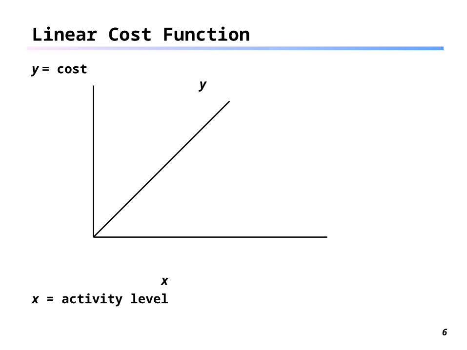
2. Cost behavior can adequately be approximated by a linear function of the activity level within the relevant range. A linear cost function is a cost function in which the graph of total
cost versus the level of a single activity is a straight line.
4
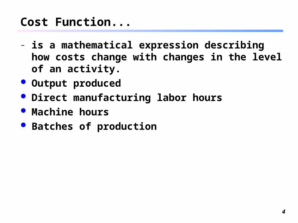
Cost Function...
– is a mathematical expression describing how costs change with changes in the level of an activity.
Output produced Direct manufacturing labor hours Machine hours Batches of production

5
Cost Function
La Bella Hotel offers Happy Airline three alternative cost structures to accommodate its crew overnight:
$60 per night per room usage Total room usage is the only factor whose change causes a
change in total costs. The cost is variable.
$8,000 per month The total cost will be $8,000 per month regardless of room usage. The cost is fixed, not variable.
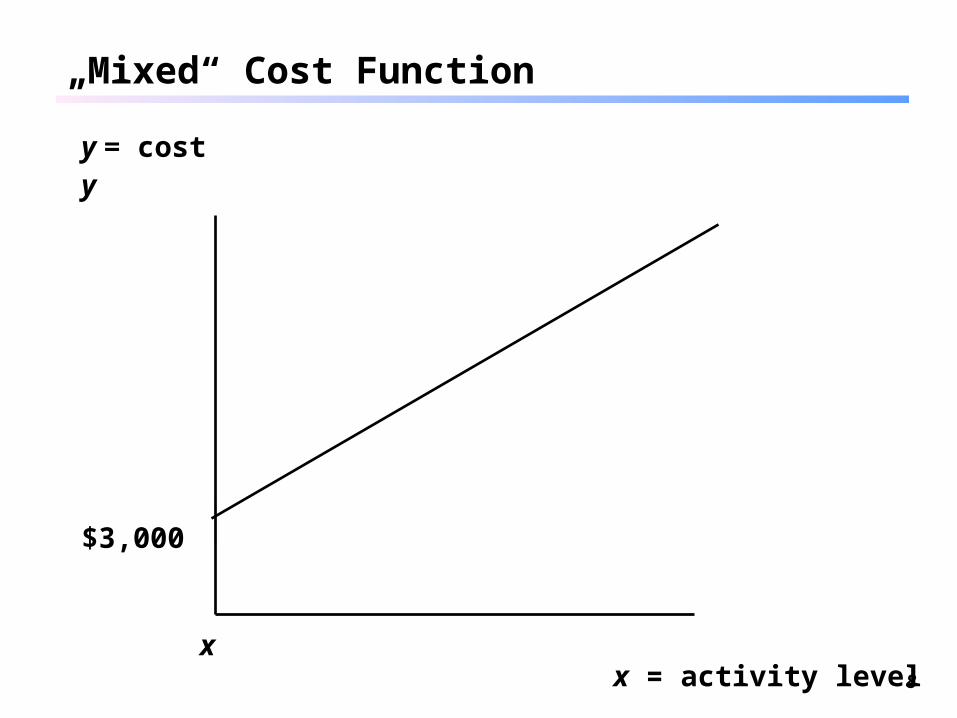
$3,000 per month plus $24 per room This is an example of a mixed cost.
What are the cost functions?
6
Linear Cost Function
y = cost y
x
x = activity level

7
Constant Cost Function
y = cost y
$8,000 x x = activity level
8
„Mixed“ Cost Function
y = cost y
$3,000
x
x = activity level

9
Cost Classification and Estimation
– Choice of cost object A cost item may be variable with respect to one cost object
and fixed with respect to another. Example: If the number of taxis owned by a taxi company is
the cost object, annual taxi registration, and license costs would be a variable cost.
If miles driven during a year on a particular taxi is the cost object, registration, and license costs for that taxi is a fixed cost.
– Time span Whether a cost is variable or fixed with respect to a
particular activity depends on the time span. More costs are variable with longer time spans.
– Relevant range

10
Relevant Range
Variable and fixed cost behavior patterns are valid for linear cost functions only within the given relevant range. Costs may behave nonlinear outside the range.
pseudo-fixedcost
11
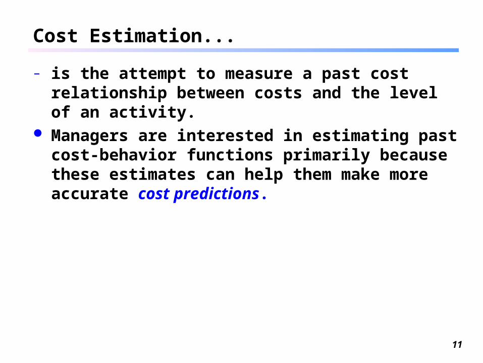
Cost Estimation...
– is the attempt to measure a past cost relationship between costs and the level of an activity.
Managers are interested in estimating past cost-behavior functions primarily because these estimates can help them make more accurate cost predictions.

12
The Cause-and-Effect Criterion In Choosing Cost Drivers
– Physical relationship (materials costs)– Contractual agreements (phone charges based on
minutes)– Implicitly established by logic (ordering costs driven
by number of parts)
13
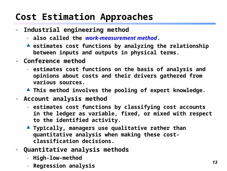
Cost Estimation Approaches– Industrial engineering method
– also called the work-measurement method. estimates cost functions by analyzing the relationship between
inputs and outputs in physical terms.
– Conference method– estimates cost functions on the basis of analysis and opinions
about costs and their drivers gathered from various sources. This method involves the pooling of expert knowledge.
– Account analysis method– estimates cost functions by classifying cost accounts in the ledger
as variable, fixed, or mixed with respect to the identified activity. Typically, managers use qualitative rather than quantitative
analysis when making these cost-classification decisions.
– Quantitative analysis methods– High-low-method– Regression analysis

14
Account Analysis
Managers use judgment and experience to decompose different cost categories in different accounts
Example: Quatisha & Co. sells software programs. Total sales = $390,000 The company sold 1,000 programs. Cost of goods sold = $130,000 Manager’s salary = $60,000 Secretary’s salary = $29,000 Commissions = 12% of sales the total fixed cost = $60,000 + $29,000 = $89,000
Classify these items according to fixed, proportional and mixed, and explain how to decompose mixed costs into fixed and variable components

15
Quantitative Analysis Methods
Quantitative analysis uses a formal mathematical method to fit linear cost functions to past data observations.
Steps in Estimating a Cost Function1 Choose the dependent variable.2 Identify the independent variable cost driver(s).3 Collect data on the dependent variable and the cost
driver(s).4 Plot the data.5 Estimate the cost function.6 Evaluate the estimated cost function.

16
1 Choose the dependent variable. Choice of the dependent variable (the cost to be predicted) will
depend on the purpose for estimating a cost function.
2 Identify the independent variable cost driver(s). The independent variable (level of activity or cost driver) is the
factor used to predict the dependent variable (costs). Requirements
A It should have an economically plausible relationship with the dependent variable.
B It should be accurately measurable. 3. Collect data on the dependent variable and the cost
driver(s). Cost analysts obtain data from company documents, from
interviews with managers, and through special studies.– Time-series data– Cross-sectional data

17
4 Plot the data. The general relationship between the cost driver and the
dependent variable can readily be observed in a plot of the data.
The plot highlights extreme observations that analysts should check.
Cost of Cost of activityactivity
Level of activityLevel of activity
Estimated cost functionEstimated cost function
Fixed cost Fixed cost
18
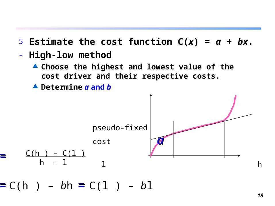
5 Estimate the cost function C(x) = a + bx.– High-low method
Choose the highest and lowest value of the cost driver and their respective costs.
Determine a and b
pseudo-fixed
cost aa
l h bb ==
aa == C(h ) – bh == C(l ) – bl
C(h ) – C(l ) h – l
19
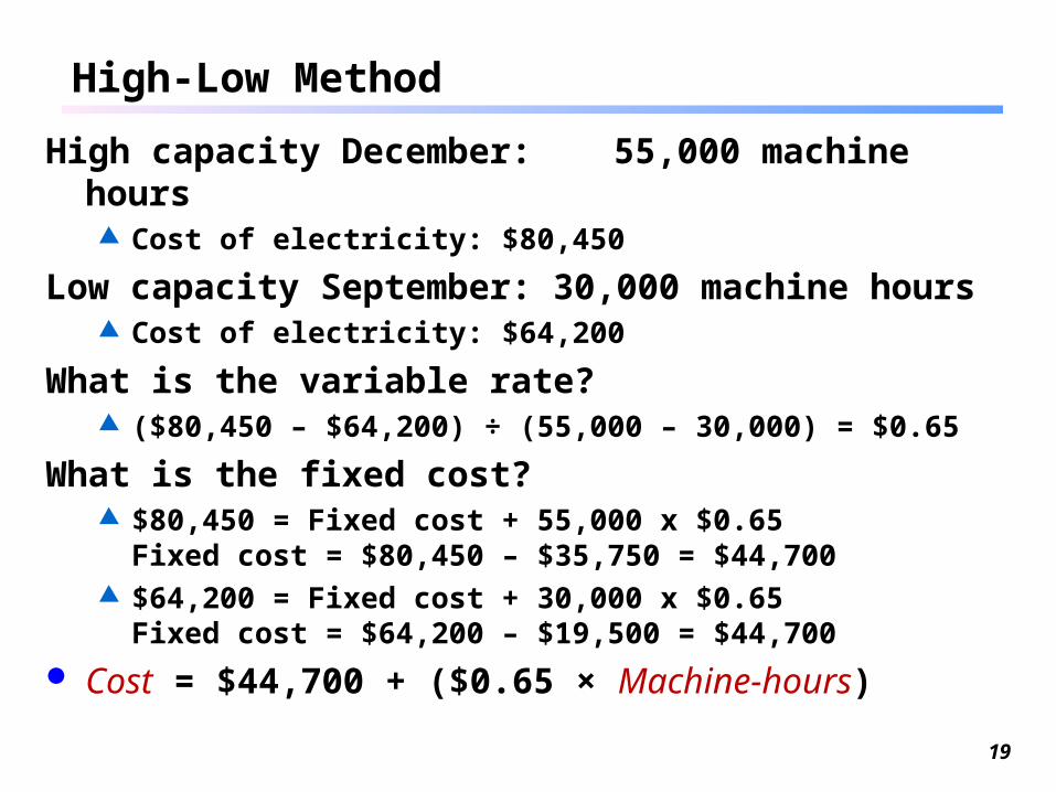
High-Low Method
High capacity December: 55,000 machine hours Cost of electricity: $80,450
Low capacity September: 30,000 machine hours Cost of electricity: $64,200
What is the variable rate? ($80,450 – $64,200) ÷ (55,000 – 30,000) = $0.65
What is the fixed cost? $80,450 = Fixed cost + 55,000 x $0.65
Fixed cost = $80,450 – $35,750 = $44,700 $64,200 = Fixed cost + 30,000 x $0.65
Fixed cost = $64,200 – $19,500 = $44,700
Cost = $44,700 + ($0.65 × Machine-hours)

20
Regression Analysis...
– is used to measure the average amount of change in a dependent variable, such as electricity, that is associated with unit increases in the amounts of one or more independent variables, such as machine hours.
Regression analysis uses all available data to estimate the cost function. Simple regression analysis estimates the relationship
between the dependent variable and one independent variable.
Multiple regression analysis estimates the relationship between the dependent variable and multiple independent variables.
21
Regression Analysis
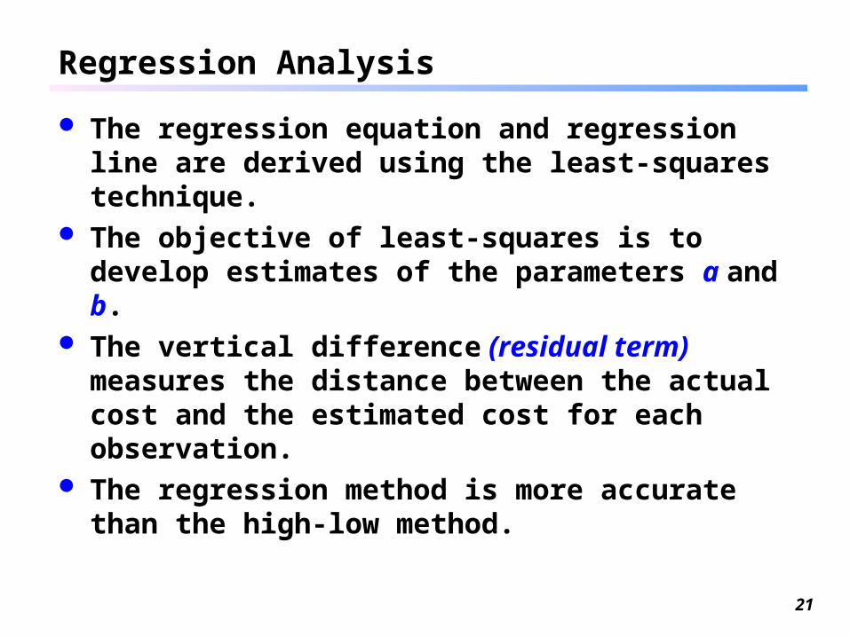
The regression equation and regression line are derived using the least-squares technique.
The objective of least-squares is to develop estimates of the parameters a and b.
The vertical difference (residual term) measures the distance between the actual cost and the estimated cost for each observation.
The regression method is more accurate than the high-low method.
22
6. Evaluate the estimated cost function.
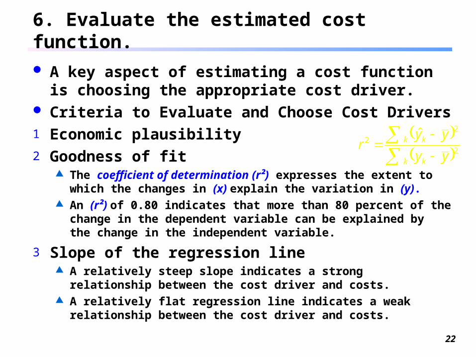
A key aspect of estimating a cost function is choosing the appropriate cost driver.
Criteria to Evaluate and Choose Cost Drivers1 Economic plausibility2 Goodness of fit
The coefficient of determination (r²) expresses the extent to which the changes in (x) explain the variation in (y).
An (r²) of 0.80 indicates that more than 80 percent of the change in the dependent variable can be explained by the change in the independent variable.
3 Slope of the regression line A relatively steep slope indicates a strong relationship between
the cost driver and costs. A relatively flat regression line indicates a weak relationship
between the cost driver and costs.
2
22 ˆ
yy
yyr
kk
kk

23
Nonlinearity and Cost Functions A nonlinear cost function is a cost function in which the graph of
total costs versus the level of a single activity is not a straight line within the relevant range.
– Economies of scale– Economies of scale in advertising may enable an advertising agency
to double the number of advertisements for less than double the cost.
– Quantity discounts– Quantity discounts on direct materials purchases produce a lower
cost per unit purchased with larger orders.– Learning Curves / Experience Curve
– a function that shows how labor-hours per unit decline as units of output increase.
a function that shows how the costs per unit in various value chain areas decline as units produced and sold increase.
Step cost functions cost is constant over various ranges of the level of activity, but the
cost increases by discrete amounts as the level of activity changes from one range to the next.

24
Learning Models
Cumulative Average Time Learning Model: Cumulative average time per unit is reduced by a
constant percentage each time the cumulative quantity of units produced is doubled.
Cumulative average time per unit =
Y/X= aXb
Incremental unit-time Learning Model: The time needed to produce the last unit is
reduced by a constant percentage each time the cumulative quantity of units produced is doubled.
Total time for cumulative output (Y)Cumulative output (X)
dYdX
= X

25
a = 100, learning rate = 80%, X = 1,2,3,4
Cumulative Average-Time Learning Model
Incremental Unit-Time Learning Model
Number of units Cumulative average labor hours per unit
Cumulative total labor hours
Individual time for Xth unit
1 100 100 100 2 80 160 60 3 70.21 210.63 50.63 4 64 256 45.37
Number of units Individual time for Xth unit
Cumulative total labor hours
Cumulative average labor hours per unit
1 100 100 100 2 80 180 90 3 70.21 250.21 83.40 4 64 314.21 78.55

26
Data Collection and Adjustment Issues
The ideal database for cost estimation has two characteristics:
1 It contains numerous reliably measured observations of the cost driver(s) and the cost that is the dependent variable.
2 It considers many values for the cost driver that span a wide range.
Pitfalls: Time periods do not match. Fixed costs are allocated as if they were variable. Data are either not available or not reliable. Inflation may play a role. Extreme values of observations occur from errors in recording
costs. Analysts should adjust or eliminate unusual observations before
estimating a cost relationship. There is no homogeneous relationship. The relationship between the cost driver and the cost is not
stationary

27
Multivariate Regression: Tests
F-Test: Can the null hypothesis be rejected that all the estimated coefficients are zero?
t-Test: Is a single cost driver „significant“? means: is the estimated b-value for the cost driver greater
than its standard error (the expected random effects on the estimate, according to the assumed normal error distribution) ?
Durbin-Watson Test: independence of residuals, autocorrelation
Linearity: look at the plot Goldfeldt-Quandt Test: Heteroscedasticity would
lead to erroneous estimated standard errors Multicollinearity: cost drivers in a multivariate
regression are correlated: standard errors are over estimated; t-Test disturbed.
28
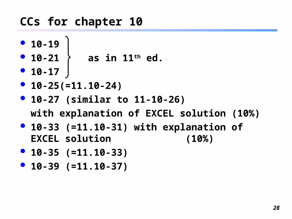
CCs for chapter 10
10-19 10-21 as in 11th ed. 10-17 10-25(=11.10-24) 10-27 (similar to 11-10-26)
with explanation of EXCEL solution (10%)
10-33 (=11.10-31) with explanation of EXCEL solution
(10%) 10-35 (=11.10-33) 10-39 (=11.10-37)

29
Data for 10-35
First PT109: $ Direct materials 100,000 Direct manuf. labor 300,000 Tooling cost 50,000 variable MOH ($20 per dmlhr) other MOH (25% of Direct manuf. labor) seven further units to be built, 85% learning curve
(b = 0.2345)


