Chapter 10 Finite-State Markov Chains - Winthrop...

Chapter 10

Finite-State Markov Chains

Introductory Example: Googling Markov Chains

Google means many things: it is an Internet search engine, the company that produces the searchengine, and a verb meaning to search on the Internet for a piece of information. Although it mayseem hard to believe, there was a time before people could “google” to find the capital of Botswana,or a recipe for deviled eggs, or other vitally important matters. Users of the Internet depend ontrustworthy search engines – the amount of available information is so vast that the searcher relieson the search engine not only to find those webpages that contain the terms of the search, but alsoto return first those webpages most likely to be relevant to the search. Early search engines had nogood way of determining which pages were more likely to be relevant. Searchers had to check thereturned pages one by one, which was a tedious and frustrating process. This situation improvedmarkedly in 1998, when search engines began to use the information contained in the hyperlinkedstructure of the World Wide Web to help to rank pages. Foremost among this new generationof search engines was Google, a project of two computer science graduate students at StanfordUniversity: Sergey Brin and Lawrence Page.

Brin and Page reasoned that a webpage was important if it had hyperlinks to it from other importantpages. They used the idea of random surfer: a web surfer moving from webpage to webpagemerely by choosing at random which hyperlink to follow. The motion of the surfer among thewebpages can be modeled using Markov chains, which were introduced in Section 4.9. The pagesthat this random surfer visits more often ought to be more important, and thus more relevant if theircontent matches the terms of a search. Although Brin and Page did not not know it at the time,they were attempting to find the steady-state vector for a particular Markov chain whose transitionmatrix modeled the hyperlinked structure of the web. After some important modifications to thisimpressively large matrix (detailed in Section 10.2), a steady-state vector can be found, and itsentries can be interpreted as the amount of time a random surfer will spend at each webpage. Thecalculation of this steady-state vector is the basis for Google’s PageRank algorithm.

So the next time you google the capital of Botswana, know that you are using the results of thischapter to find just the right webpage.

1

Even though the number of webpages is huge, it is still finite. When the link structure of the WorldWide Web is modeled by a Markov chain, each webpage is a state of the Markov chain. Thischapter continues the study of Markov chains begun in Section 4.9, focusing on those Markovchains with a finite number of states. Section 10.1 introduces useful terminology and developssome examples of Markov chains: signal transmission models, diffusion models from physics, andrandom walks on various sets. Random walks on directed graphs will have particular application tothe PageRank algorithm. Section 10.2 defines the steady-state vector for a Markov chain. Althoughall Markov chains have a steady-state vector, not all Markov chains converge to a steady-statevector. When the Markov chain converges to a steady-state vector, that vector can be interpretedas telling the amount of time the chain will spend in each state. This interpretation is necessary forthe PageRank algorithm, so the conditions under which a Markov chain converges to a steady-statevector will be developed. The model for the link structure of the World Wide Web will then bemodified to meet these conditions, forming what is called the Google matrix. Sections 10.3 and10.4 discuss Markov chains that do not converge to a steady-state vector. These Markov chainscan be used to model situations in which the chain eventually becomes confined to one state or aset of states. Section 10.5 introduces the fundamental matrix. This matrix can be used to calculatethe expected number of steps it takes the chain to move from one state to another, as well as theprobability that the chain ends up confined to a particular state. In Section 10.6, the fundamentalmatrix is applied to a model for run production in baseball: the number of batters in a half inningand the state in which the half inning ends will be of vital importance in calculating the expectednumber of runs scored.

10.1 Introduction and Examples 3

10.1 Introduction and Examples

Recall from Section 4.9 that aMarkov chain is a mathematical model for movement betweenstates. A process starts in one of these states and moves from state to state. The moves betweenstates are calledstepsor transitions. The terms “chain” and “process” are used interchangeably,so the chain can be said to move between states and to be “at a state” or “in a state” after a certainnumber of steps.

The state of the chain at any given step is not known; what is known is the probability that thechain moves from statej to statei in one step. This probability is called atransition probabilityfor the Markov chain. The transition probabilities are placed in a matrix called thetransitionmatrix P for the chain by entering the probability of a transition from statej to statei at the(i, j)-entry ofP . So if there werem states named1, 2, . . .m, the transition matrix would be them×m matrix

P =

From:1 j m To:

... 1

↓pij · · · → i

m

The probabilities that the chain is in each of the possible states aftern steps are listed in astatevector xn. If there arem possible states the state vector would be

xn =

a1...aj...

am

←− Probability that the chain is at statej aftern steps

State vectors areprobability vectors since their entries must sum to1. The state vectorx0 is calledthe initial probability vector .

Notice that thejth column ofP is a probability vector – its entries list the probabilities of amove from statej to the states of the Markov chain. The transition matrix is thus astochasticmatrix since all of its columns are probability vectors.

The state vectors for the chain are related by the equation

xn+1 = Pxn (1)

for n = 1, 2, . . .. Notice that Equation (1) may be used to show that

xn = P nx0 (2)

Thus any state vectorxn may be computed from the initial probability vectorx0 and an appropriatepower of the transition matrixP .

4 CHAPTER 10 Finite-State Markov Chains

This chapter concerns itself with Markov chains with a finite number of states; that is, thosechains for which the transition matrixP is of finite size. To use a finite-state Markov chain tomodel a process, the process must have the following properties, which are implied by Equations(1) and (2).

1. Since the values in the vectorxn+1 depend only on the transition matrixP and onxn, thestate of the chain before timen must have no effect on its state at timen + 1 and beyond.

2. Since the transition matrixP does not change with time, the probability of a transition fromone state to another must not depend upon how many steps the chain has taken.

Even with these restrictions, Markov chains may be used to model an amazing variety of processes.Here is a sampling.

Signal Transmission

Consider the problem of transmitting a signal along a telephone line or by radio waves. Eachpiece of data must pass through a multi-stage process to be transmitted, and at each stage thereis a probability that a transmission error will cause the data to be corrupted. Assume that theprobability of an error in transmission is not effected by transmission errors in the past and doesnot depend on time, and that the number of possible pieces of data is finite. The transmissionprocess may then be modeled by a Markov chain. The object of interest is the probability that apiece of data goes through the entire multi-stage process without error. Here is an example of sucha model.

EXAMPLE 1 Suppose that each bit of data is either a 0 or a 1, and at each stage there is aprobabilityp that the bit will pass through the stage unchanged. Thus the probability is1− p thatthe bit will be transposed. The transmission process is modeled by a Markov chain, with states0and1 and transition matrix

P =

From:0 1 To:p 1− p 0

1− p p 1

It is often easier to visualize the action of a Markov chain by representing its transition probabilitiesgraphically as in Figure 1. The points are the states of the chain, and the arrows represent thetransitions.

Suppose thatp = .99. Find the probability that the signal 0 will still be a 0 after a 2-stagetransmission process.

Solution Since the signal begins as 0, the probability that the chain begins at 0 is 100%, or 1; thatis, the initial probability vector is

x0 =

[10

]


1 - p

1 - p

p p0 1

Figure 1: Transition diagram for signal transmission.

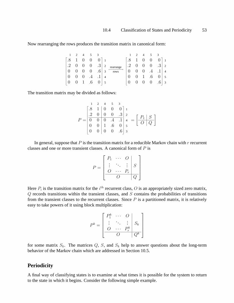
To find the probability of a two-step transition, compute

x2 = P 2x0 =

[.99 .01.01 .99

]2 [10

]=

[.9802 .0198.0198 .9802

] [10

]=

[.9802.0198

]The probability that the signal 0 will still be a 0 after the 2-stage process is thus.9802. Noticethat this is not the same as the probability that the 0 is transmitted without error; that probabilitywould be(.99)2 = .9801. Our analysis includes the very small probability that the 0 is erroneouslychanged to 1 in the first step, then back to 0 in the second step of transmission. �

Diffusion

Consider two compartments filled with different gases which are separated only by a membranewhich allows molecules of each gas to pass from one container to the other. The two gases willthen diffuse into each other over time, so that each container will contain some mixture of thegases. The major question of interest is what mixture of gases is in each container at a time afterthe containers are joined. A famous mathematical model for this process was described originallyby the physicists Paul and Tatyana Ehrenfest. Since their preferred term for “container” was urn,the model is called theEhrenfest urn model for diffusion.

Label the two urnsA andB, and placek molecules of gas in each urn. At each time step, selectone of the2k molecules at random and move it from its urn to the other urn, and keep track of thenumber of molecules in urnA. This process can be modeled by a finite-state Markov chain: thenumber of molecules in urnA aftern + 1 time steps depends only on the number in urnA afterntime steps, the transition probabilities do not change with time, and the number of states is finite.

EXAMPLE 2 For this example, letk = 3. Then the two urns contain a total of6 molecules, andthe possible states for the Markov chain are0, 1, 2, 3, 4, 5, and6. Notice first that if there are0molecules in urnA at timen, then there must be1 molecule in urnA at timen+1, and if there are6 molecules in urnA at timen, then there must be5 molecules in urnA at timen + 1. In terms of


the transition matrixP , this means that the columns inP corresponding to states0 and6 are

p0 =

0100000

andp6 =

0000010

If there arei molecules in urnA at timen, with 0 < i < 6, then there must be eitheri − 1 ori + 1 molecules in urnA at timen + 1. In order for a transition fromi to i− 1 molecules to occur,one of thei molecules in urnA must be selected to move; this event happens with probabilityi/6.Likewise a transition fromi to i + 1 molecules occurs when one of the6 − i molecules in urnBis selected, and this occurs with probability(6− i)/6. Allowing i to range from1 to 5 creates thecolumns ofP corresponding to these states, and the transition matrix for the Ehrenfest urn modelwith k = 3 is thus

P =

0 1 2 3 4 5 6

0 1/6 0 0 0 0 0 0

1 0 1/3 0 0 0 0 1

0 5/6 0 1/2 0 0 0 2

0 0 2/3 0 2/3 0 0 3

0 0 0 1/2 0 5/6 0 4

0 0 0 0 1/3 0 1 5

0 0 0 0 0 1/6 0 6

Figure 2 shows a transition diagram of this Markov chain. Another model for diffusion will beconsidered in the Exercises for this section. �

1

5

6

2

3

1

2

1

3

1

6

1

6

1

3

1

2

2

3

5

6

1

0 1 2 3 4 5 6

Figure 2: Transition diagram of the Ehrenfest urn model.

Random Walks on{1, . . . , n}Molecular motion has long been an important issue in physics. Einstein and others investigatedBrownian motion, which is a mathematical model for the motion of a molecule exposed to colli-sions with other molecules. The analysis of Brownian motion turns out to be quite complicated,


but a discrete version of Brownian motion called arandom walk provides an introduction to thisimportant model. Think of the states{1, 2, . . . , n} as lying on a line. Place a molecule at a pointthat is not on the end of the line. At each step the molecule moves left one unit with probabilityp and right one unit with probability1 − p. See Figure 3. The molecule thus “walks randomly”along the line. Ifp = 1/2, the walk is calledsimple, or unbiased. If p 6= 1/2, the walk is said tobebiased.

1 - p 1 - p 1 - p 1 - p

p p p p

... k-2 k-1 k k+1 k+2 ...

Figure 3: A graphical representation of a random walk.

The molecule must move either to the left or right at the states2, . . . , n − 1, but it cannot dothis at the endpoints1 andn. The molecule’s possible movements at the endpoints1 andn must bespecified. One possibility is to have the molecule stay at an endpoint forever once it reaches eitherend of the line. This is called arandom walk with absorbing boundaries, and the endpoints1andn are calledabsorbing states. Another possibility is to have the molecule bounce back oneunit when an endpoint is reached. This is called arandom walk with reflecting boundaries.

EXAMPLE 3 A random walk on{1, 2, 3, 4, 5} with absorbing boundaries has a transition matrixof

P =

1 2 3 4 5

1 p 0 0 0 1

0 0 p 0 0 2

0 1− p 0 p 0 3

0 0 1− p 0 0 4

0 0 0 1− p 1 5

since the molecule at state1 has probability1 of staying at state1, and a molecule at state5 hasprobability1 of staying at state5. A random walk on{1, 2, 3, 4, 5} with reflecting boundaries hasa transition matrix of

P =

1 2 3 4 5

0 p 0 0 0 1

1 0 p 0 0 2

0 1− p 0 p 0 3

0 0 1− p 0 1 4

0 0 0 1− p 0 5

since the molecule at state1 has probability1 of moving to state2, and a molecule at state5 hasprobability1 of moving to state4. �

In addition to their use in physics, random walks also occur in problems related to gamblingand its more socially acceptable variants: the stock market and the insurance industry.


EXAMPLE 4 Consider a very simple casino game. A gambler (who still has some money leftwith which to gamble) flips a fair coin and calls heads or tails. If the gambler is correct, he wins adollar; if he is wrong, he loses a dollar. Suppose that the gambler will quit the game when eitherhe has wonn dollars or has lost all of his money.

Suppose thatn = 7 and the gambler starts with $4. Notice that the gambler’s winnings moveeither up or down $1 at each move, and once the gambler’s winnings reach0 or 7, they do notchange any more since the gambler has quit the game. Thus the gambler’s winnings may bemodeled by a random walk with absorbing boundaries and states{0, 1, 2, 3, 4, 5, 6, 7}. Since amove up or down is equally likely in this case,p = 1/2 and the walk is simple.

Random Walk on Graphs

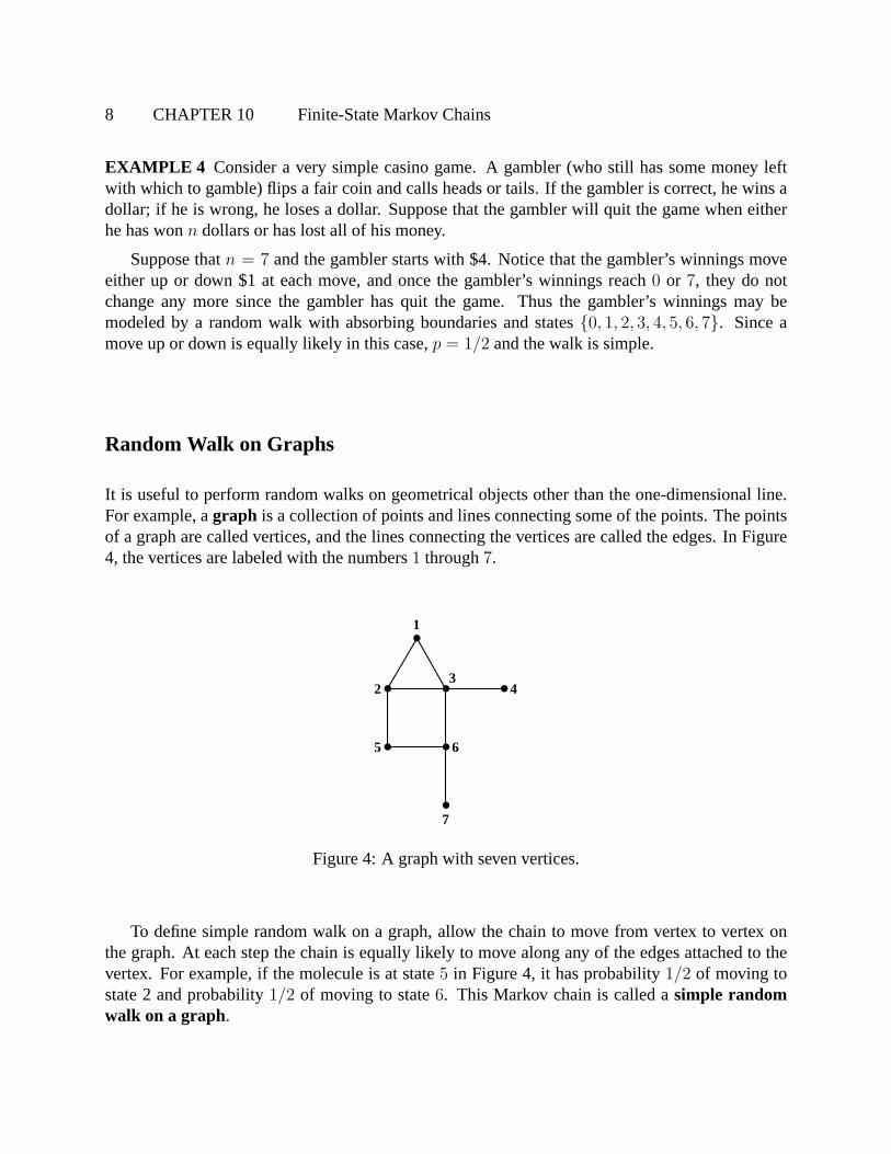
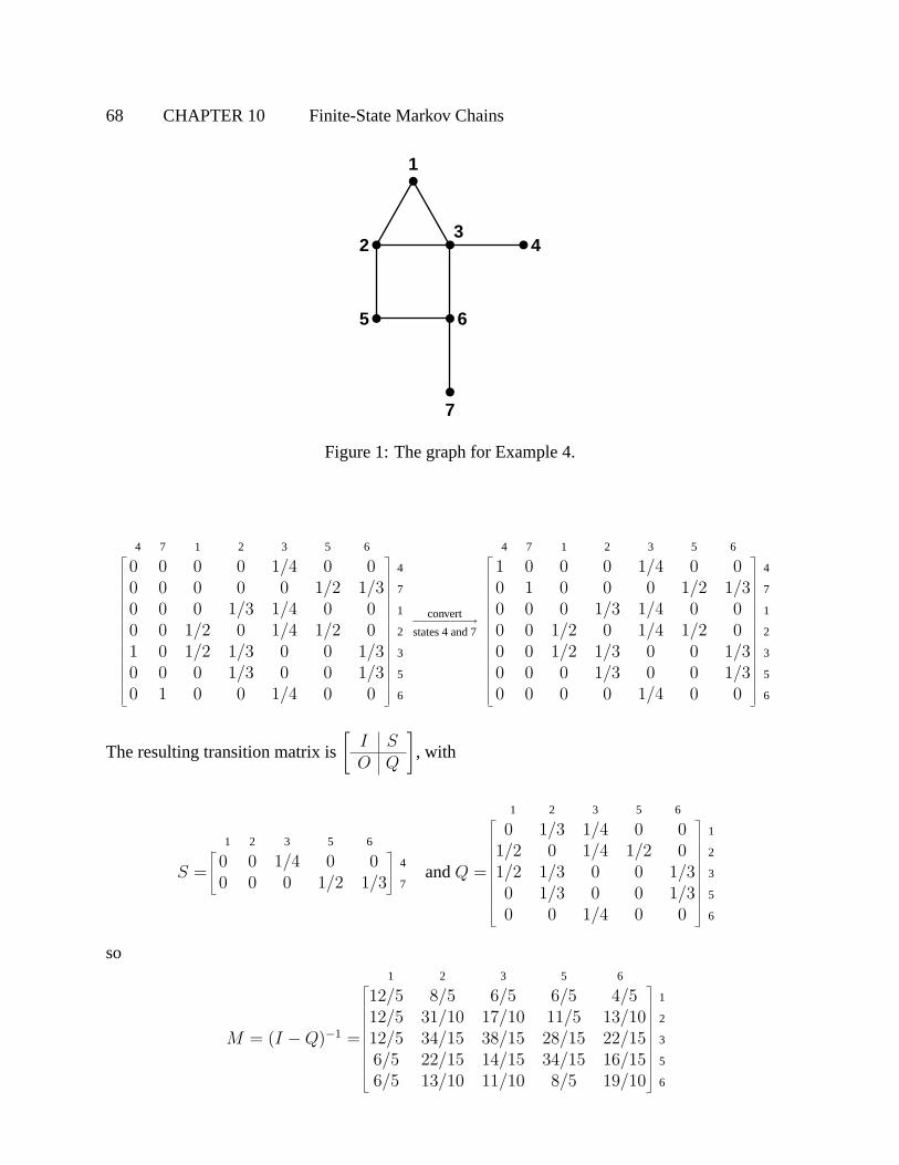
It is useful to perform random walks on geometrical objects other than the one-dimensional line.For example, agraph is a collection of points and lines connecting some of the points. The pointsof a graph are called vertices, and the lines connecting the vertices are called the edges. In Figure4, the vertices are labeled with the numbers1 through7.

1

2

3

4

5 6

7

Figure 4: A graph with seven vertices.

To define simple random walk on a graph, allow the chain to move from vertex to vertex onthe graph. At each step the chain is equally likely to move along any of the edges attached to thevertex. For example, if the molecule is at state5 in Figure 4, it has probability1/2 of moving tostate 2 and probability1/2 of moving to state6. This Markov chain is called asimple randomwalk on a graph.


EXAMPLE 5 Simple random walk on the graph in Figure 4 has transition matrix

P =

1 2 3 4 5 6 7

0 1/3 1/4 0 0 0 0 1

1/2 0 1/4 0 1/2 0 0 2

1/2 1/3 0 1 0 1/3 0 3

0 0 1/4 0 0 0 0 4

0 1/3 1/4 0 0 1/3 0 5

0 0 0 0 1/2 0 1 6

0 0 0 0 0 1/3 0 7

Find the probability that the chain in Figure 4 moves from state6 to state2 in exactly3 steps.

Solution Compute

x3 = P 3x0 = P 3

0000010

=

.0833

.0417

.40280

.27780

.1944

so the probability of moving from state6 to state2 in exactly3 steps is.0417. �

Sometimes interpreting a random process as a random walk on a graph can be useful.

EXAMPLE 6 Suppose a mouse runs through the five-room maze on the left side of Figure 5. Themouse moves to a different room at each time step. When the mouse is in a particular room, it isequally likely to choose any of the doors out of the room. Note that a Markov chain can model themotion of the mouse. Find the probability that a mouse starting in room3 returns to that room inexactly5 steps.

1 2

3 4

5

1 2

3 4

5

Figure 5: The five-room maze with overlaid graph.


Solution A graph is overlaid on the maze on the right side of Figure 5. Notice that the motion ofthe mouse is identical to simple random walk on the graph, so the transition matrix is

P =

1 2 3 4 5

0 1/3 1/4 0 0 1

1/2 0 1/4 1/3 0 2

1/2 1/3 0 1/3 1/2 3

0 1/3 1/4 0 1/2 4

0 0 1/4 1/3 0 5

and find that

x5 = P 5x0 = P 5

00100

=

.1507.2143.2701.2143.1507

Thus the probability of a return to room3 in exactly5 steps is.2701. �

Another interesting object on which to walk randomly is adirected graph. A directed graphis a graph in which the vertices are not joined by lines but by arrows. See Figure 6.

1

2

3

4

5 6

7

Figure 6: A directed graph with seven vertices.

To perform a simple random walk on a directed graph, allow the chain to move from vertex tovertex on the graph but only in the directions allowed by the arrows. At each step the walker isequally likely to move away from its current state along any of the arrows pointing away from thevertex. For example, if the molecule is at state6 in Figure 6, it has probability1/3 of moving tostate3, state5, and state7.

The PageRank algorithm which Google uses to rank the importance of pages on the WorldWide Web (see the Chapter Introduction) begins with a simple random walk on a directed graph.The Web is modeled as a directed graph where the vertices are the pages and an arrow is drawnfrom pagej to pagei if there is a hyperlink from pagej to pagei. A person surfs randomly inthe following way: when the surfer gets to a page, he or she chooses a link from the page so thatit is equally probable to choose any of the possible “outlinks.” The surfer then follows the link to


arrive at another page. The person surfing in that way is performing a simple random walk on thedirected graph that is the World Wide Web.

EXAMPLE 7 Consider a set of seven pages hyperlinked by the directed graph in Figure 6. If therandom surfer starts at page5, find the probability that the surfer is at page3 after four clicks.

Solution The transition matrix for the simple random walk on the directed graph is

P =

1 2 3 4 5 6 7

0 1/2 0 0 0 0 0 1

0 0 1/3 0 1/2 0 0 2

1 0 0 0 0 1/3 0 3

0 0 1/3 1 0 0 0 4

0 1/2 0 0 0 1/3 0 5

0 0 1/3 0 1/2 0 0 6

0 0 0 0 0 1/3 1 7

Notice that there are no arrows coming from either state4 or state7. If the surfer clicks on a link toeither of these pages, there is no link to click on next.1 For that reason, the transition probabilitiesp44 andp77 are set equal to1 – the chain must stay at state4 or state7 forever once it enters eitherof these states. Computingx4 gives

x4 = P 4x0 =

.1319

.0833

.0880

.1389

.2199

.0833

.2546

so the probability of being at3 after exactly4 clicks is .0880. �

States4 and7 are absorbing states for the Markov chain in the previous example. In technicalterms they are calleddangling nodesand are quite common on the Web – data pages in particularusually have no links leading from them. Dangling nodes will appear in the next section, wherethe PageRank algorithm will be explained.

As was noted in Section 4.9, the most interesting questions about Markov chains concern theirlong-term behavior; that is, the behavior ofxn asn increases. This study will occupy a largeportion of this chapter. The foremost issues in our study will be whether the sequence of vectors{xn} is converging to some limiting vector asn increases, and how to interpret this limiting vectorif it exists. Convergence to a limiting vector will be addressed in the next section.

1Using the “Back” key is not allowed – the state of the chain before timen must have no effect on its state at timen + 1 and beyond.


Practice Problems

1. Fill in the missing entries in the stochastic matrix

P =

.1 ∗ .2∗ .3 .3.6 .2 ∗

2. In the signal transmission model in Example 1, suppose thatp = .03. Find the probability

that the signal “1” will be a “0” after a 3-stage transmission process.


10.1 ExercisesIn Exercises 1 and 2, determine whetherP is astochastic matrix. IfP is not a stochastic matrix,explain why not.

1. a.P =

[.3 .4.7 .6

]b. P =

[.3 .7.4 .6

]

2. a.P =

[1 .50 .5

]b. P =

[.2 1.1.8 −.1

]In Exercises 3 and 4, computex3 in two ways:by computingx1 andx2, and by computingP 3.

3. P =

[.6 .5.4 .5

];x0 =

[10

]

4. P =

[.3 .8.7 .2

];x0 =

[.5.5

]In Exercises 5 and 6, the transition matrixP fora Markov chain with states0 and1 is given. As-sume that in each case the chain starts in state0 at timen = 0. Find the probability that thechain is in state1 at timen.

5. P =

[1/3 3/42/3 1/4

], n = 3

6. P =

[.4 .2.6 .8

], n = 5

In Exercises 7 and 8, the transition matrixP fora Markov chain with states0, 1 and2 is given.Assume that in each case the chain starts in state0 at timen = 0. Find the probability that thechain is in state1 at timen.

7. P =

1/3 1/4 1/21/3 1/2 1/41/3 1/4 1/4

, n = 2

8. P =

.1 .2 .4.6 .3 .4.3 .5 .2

, n = 3

9. Consider a pair of Ehrenfest urns. If thereare currently 3 molecules in one urn and5 in the other, what is the probability thatthe exact same situation will apply after

a. 4 selections?

b. 5 selections?

10. Consider a pair of Ehrenfest urns. If thereare currently no molecules in one urn and7 in the other, what is the probability thatthe exact same situation will apply after

a. 4 selections?

b. 5 selections?

11. Consider unbiased random walk on the set{1, 2, 3, 4, 5, 6}. What is the probability ofmoving from2 to3 in exactly 3 steps if thewalk has

a. reflecting boundaries?

b. absorbing boundaries?

12. Consider biased random walk on the set{1, 2, 3, 4, 5, 6} with p = 2/3. What isthe probability of moving from2 to 3 inexactly 3 steps if the walk has

a. reflecting boundaries?

b. absorbing boundaries?

In Exercises 13 and 14, find the transition matrixfor the simple random walk on the given graph.

13.1 2

34

5


14.1 2

34

In Exercises 15 and 16, find the transition ma-trix for the simple random walk on the given di-rected graph.

15.1 2

3 4

16.1

2

3

4

5

In Exercises 17 and 18, suppose a mouse wan-ders through the given maze. The mouse mustmove into a different room at each time step, andis equally likely to leave the room through anyof the available doorways.

17. The mouse is placed in room 2 of the mazebelow.

a. Construct a transition matrix and aninitial probability vector for themouse’s travels.

b. What are the probabilities that themouse is in each of the rooms after3 moves?

1 2

3

4 5




1 2 3

4 5

In Exercises 19 and 20, suppose a mouse wan-ders through the given maze some of whosedoors are “one-way”: they are just large enoughfor the mouse to squeeze through in only onedirection. The mouse still must move into a dif-ferent room at each time step if possible. Whenfaced with accessible openings into two or morerooms, the mouse chooses them with equal prob-ability.





1 2 3

4 5 6




1 2

3

4 5

In Exercises 21 and 22, mark each statementTrue or False. Justify each answer.

21. a. The columns of a transition matrixfor a Markov chain must sum to 1.

b. The transition matrixP may changeover time.

c. The(i, j)-entry in a transition matrixP gives the probability of a movefrom statej to statei.

22. a. The rows of a transition matrix for aMarkov chain must sum to 1.

b. If {xn} is a Markov chain, thenxn+1

must depend only on the transitionmatrix andxn.

c. The(i, j)-entry inP 3 gives the prob-ability of a move from statei to statej in exactly three time steps.

23. The weather in Charlotte, North Carolinacan be classified as either sunny, cloudy,or rainy on a given day. Climate data from20032 reveal the following facts:

• If a day is sunny, then the next dayis sunny with probability .65, cloudywith probability .1, and rainy withprobability .25.

• If a day is cloudy, then the next dayis sunny with probability .25, cloudywith probability .25, and rainy withprobability .5.

• If a day is rainy, then the next dayis sunny with probability .25, cloudywith probability .15, and rainy withprobability .60.

Suppose it is cloudy on Monday. Use aMarkov chain to find the probabilities ofthe different kinds of possible weather onFriday.

24. Suppose that whether it rains in Charlottetomorrow depends on the weather condi-tions for today and yesterday. Climate datain 20031 show that

• If it rained yesterday and today, thenit will rain tomorrow with probabil-ity .58.

2http://www.wunderground.com/history/airport/KCLT/2003/1/1/MonthlyHistory.html


• If it rained yesterday but not today,then it will rain tomorrow with prob-ability .29.

• If it rained today but not yesterday,then it will rain tomorrow with prob-ability .47.

• If it did not rain yesterday and today,then it will rain tomorrow with prob-ability .31.

Even though the weather depends on thelast two days in this case, we can create aMarkov chain model using the states

1 it rained yesterday and today2 it rained yesterday but not today3 it rained today but not yesterday4 it did not rain yesterday and today

So, for example, the probability of a tran-sition from state 1 to state 1 is.58, and thetransition from state 1 to state 3 is0.

a. Complete the creation of the transi-tion matrix for this Markov chain.

b. If it rains on Tuesday and is clear onWednesday, what is the probabilityof no rain on the next weekend?

25. Consider a set of four webpages hyper-linked by the directed graph in Exercise15. If a random surfer starts at page 1,what is the probability that the surfer is ateach of the pages after 3 clicks?

26. Consider a set of five webpages hyper-linked by the directed graph in Exercise16. If a random surfer starts at page 2,what is the probability that the surfer is ateach of the pages after 4 clicks?

27. Consider a model for signal transmissionwhere data is sent as two-bit bytes. Thenthere are four possible bytes 00, 01, 10,and 11 which are the states of the Markov

chain. At each stage there is a probabilityp that each bit will pass through the stageunchanged.

a. Construct the transition matrix forthe model.

b. Suppose thatp = .99. Find the prob-ability that the signal “01” will stillbe “01” after a three-stage transmis-sion.

28. Consider a model for signal transmissionwhere data is sent as three-bit bytes. Con-struct the transition matrix for the model.

29. Another version of the Ehrenfest modelfor diffusion starts withk molecules of gasin each urn. One of the2k molecules ispicked at random just as in the Ehrenfestmodel in the text. The chosen molecule isthen moved to the other urn with a fixedprobabilityp and is placed back in its urnwith probability1−p. (Note that the Ehren-fest model in the text is this model withp = 1.)

a. Letk = 3. Find the transition matrixfor this model.

b. Let k = 3 and p = 1/2. If thereare currently no balls in UrnA, whatis the probability that there will be3balls in UrnA after5 selections?

30. Another model for diffusion is called theBernoulli-LaPlacemodel. Two urns (UrnA and UrnB) contain a total of2k mole-cules. In this case,k of the molecules areof one type (called Type I molecules) andk are of another type (Type II molecules).In addition,k molecules must be in eachurn all times. At each time step, a pairof molecules is selected, one from UrnAand one from UrnB, and these moleculeschange urns. Let the Markov chain model


the number of Type I molecules in UrnA (which is also the number of Type IImolecules in UrnB).

a. Suppose that there arej Type I mole-cules in UrnA with 0 < j < k. Ex-plain why the probability of a tran-sition to j − 1 Type I molecules inUrn A is (j/k)2, and why the proba-bility of a transition toj + 1 Type Imolecules in UrnA is ((k − j)/k)2.

b. Let k = 5. Use the result in parta. to set up the transition matrix forthe Markov chain which models thenumber of Type I molecules in UrnA.

c. Letk = 5 and begin with all Type Imolecules in UrnA. What is the dis-tribution of Type I molecules after 3time steps?

31. To win a game in tennis, one player mustscore four points and must also score atleast two points more than his or her oppo-nent. Thus if the two players have scoredan equal number of points (which is called“deuce” in tennis jargon), one player mustthen score two points in a row to win thegame. Suppose that players A and B areplaying a game of tennis which is at deuce.If A wins the next point, it is called “ad-vantage A” while if B wins the point it is“advantage B.” If the game is at advantageA and player A wins the next point, thenplayer A wins the game. If player B winsthe point at advantage A the game is backat deuce.

a. Suppose that the probability that Awins any point isp. Model the prog-ress of a tennis game starting at deuceusing a Markov chain with the fivestates

1 deuce2 advantage A3 advantage B4 A wins the game5 B wins the game

Find the transition matrix for thisMarkov chain.

b. Letp = .6. Find the probability thatthe game is at “advantage B” afterthree points starting at deuce.

32. Volleyball uses two different scoring sys-tems in which a team must win by at leasttwo points. In both systems, arally beginswith a serve by one of the teams and endswhen the ball goes out of play, touches thefloor, or a player commits a fault. Theteam that wins the rally gets to serve forthe next rally. Games are played to 15, 25or 30 points.

a. In rally point scoringthe team thatwins a rally is awarded a point nomatter which team served for therally. Assume that team A has prob-ability p of winning a rally for whichit serves, and that team B has proba-bility q of winning a rally for whichit serves. Model the progress of avolleyball game using a Markov chainwith the six states1 tied – A serving2 tied – B serving3 A ahead by 1 point – A serving4 B ahead by 1 point – B serving5 A wins the game6 B wins the game


b. Suppose that team A and team B aretied 15-15 in a 15-point game andthat team A is serving. Letp = q =.6. Find the probability that the gameis not finished after three rallies.


c. Inside out scoringthe team that winsa rally is awarded a point only whenit served for the rally. Assume thatteam A has probabilityp of winninga rally for which it serves, and thatteam B has probabilityq of winninga rally for which it serves. Model theprogress of a volleyball game usinga Markov chain with the eight states1 tied – A serving2 tied – B serving3 A ahead by 1 point – A serving4 A ahead by 1 point – B serving5 B ahead by 1 point – A serving6 B ahead by 1 point – B serving7 A wins the game8 B wins the game


d. Suppose that team A and team B aretied 15-15 in a 15-point game andthat team A is serving. Letp = q =.6. Find the probability that the gameis not finished after three rallies.

33. Suppose thatP is a stochastic matrix allof whose entries are greater than or equalto p. Show that all of the entries inP n aregreater than or equal top for n = 1, 2, . . ..


Solutions to Practice Problems

1. Since a stochastic matrix must have columns that sum to1,

P =

.1 .5 .2.3 .3 .3.6 .2 .5

2. The transition matrix for the model is

P =

[.97 .03.03 .97

]Since the signal begins as “1”, the initial probability vector is

x0 =

[01

]To find the probability of a three-step transition, compute

x2 = P 3x0 =

[.9153 .0847.0847 .9153

] [01

]=

[.0847.9153

]The probability of a change to “0” is thus.0847.


10.2 The Steady-State Vector and Google’s PageRank

As was seen in Section 4.9, the most interesting aspect of a Markov chain is its long-range behavior:the behavior ofxn asn increases without bound. In many cases, the sequence of vectors{xn} isconverging to a vector which is called thesteady-state vectorfor the Markov chain. This sectionwill review how to compute the steady-state vector of a Markov chain, explain how to interpretthis vector if it exists, and will offer an expanded version of Theorem 18 in Section 4.9, whichdescribes the circumstances under which{xn} converges to a steady-state vector. This Theoremwill be applied to the Markov chain model used for the World Wide Web in the previous sectionand will show how the PageRank method for ordering the importance of webpages is derived.

Steady-State Vectors

In many cases, the Markov chainxn and the matrixP n change very little for large values ofn.

EXAMPLE 1 To begin, recall Example 3 from Section 4.9. That example concerned a Markov

chain with transition matrixP =

.5 .2 .3.3 .8 .3.2 0 .4

and initial probability vectorx0 =

100

. The

vectorsxn were seen to be converging to the vectorq =

.3.6.1

. This result may be written as

limn→∞

xn = q. Increasing powers of the transition matrixP may also be computed, giving:

P 2 =

.3700 .2600 .3300.4500 .7000 .4500.1800 .0400 .2200

P 3 =

.3290 .2820 .3210.5250 .6500 .5250.1460 .0680 .1540

P 4 =

.3133 .2914 .3117.5625 .6250 .5625.1242 .0836 .1258

P 5 =

.3064 .2958 .3061.5813 .6125 .5813.1123 .0917 .1127

P 10 =

.3002 .2999 .3002.5994 .6004 .5994.1004 .0997 .1004

P 15 =

.3000 .3000 .3000.6000 .6000 .6000.1000 .1000 .1000

so the sequence of matrices{P n} also seems to be converging to a matrix asn increases, and thismatrix has the unusual property that all of its columns equalq. The example also showed thatPq = q. This equation forms the definition for the steady-state vector, and is a straightforwardway to calculate it.

DEFINITION If P is a stochastic matrix, then asteady-state vector(or equilibrium vector orinvariant probability vector ) for P is a probability vectorq such that

Pq = q

10.2 The Steady-State Vector and Google’s PageRank 21

Exercises 36 and 37 will show that every stochastic matrixP has a steady-state vectorq. Noticethat1 must be an eigenvalue of any stochastic matrix, and the steady-state vector is a probabilityvector which is also an eigenvector ofP associated with the eigenvalue1.

Although the definition of the steady-state vector makes the calculation ofq straightforward, ithas a major drawback: there are Markov chains which have a steady-state vectorq but for whichlim

n→∞xn 6= q: the definition is not sufficient forxn to converge. Examples 3-5 below will show

different ways in whichxn can fail to converge – later in this section the conditions under whichlim

n→∞xn = q will be restated. For now, consider whatq means whenlim

n→∞xn = q, as it does in the

example above. Whenlimn→∞

xn = q there are two ways to interpret this vector.

• Sincexn is approximately equal toq for largen,the entries inq approximate the probabilitythat the chain is in each state aftern time steps. Thus in the above example, no matter thevalue of the initial probability vector, after many steps the probability that the chain is instate 1 is approximatelyq1 = .3. Likewise the probability that the chain is in state 2 in thedistant future is approximatelyq2 = .6, and the probability that the chain is in state 3 in thedistant future is approximatelyq3 = .1. So the entries inq give long-run probabilities .

• WhenN is large,q approximatesxn for almost all values ofn ≤ N . Thus the entries inqapproximate the proportion of time steps that the chain spends in each state. In the aboveexample, the chain will end up spending.3 of the time steps in state 1,.6 of the time steps instate 2, and.1 of the time steps in state 2. So the entries inq give the proportion of the timesteps spent in each state, which are called theoccupation timesfor each state.

EXAMPLE 2 For an application of computingq, consider the rat-in-the-maze example (Example6, Section 10.1). In this example, the position of a rat in a five-room maze is modeled by a Markovchain with states{1, 2, 3, 4, 5} and transition matrix

P =

1 2 3 4 5

0 1/3 1/4 0 0 1

1/2 0 1/4 1/3 0 2

1/2 1/3 0 1/3 1/2 3

0 1/3 1/4 0 1/2 4

0 0 1/4 1/3 0 5

The steady-state vector may be computed by solving the systemPq = q, which is equivalent tothe homogeneous system(P − I)q = 0. Row reduction gives

−1 1/3 1/4 0 0 01/2 −1 1/4 1/3 0 01/2 1/3 −1 1/3 1/2 00 1/3 1/4 −1 1/2 00 0 1/4 1/3 −1 0

∼

1 0 0 0 −1 00 1 0 0 −3/2 00 0 1 0 −2 00 0 0 1 −3/2 00 0 0 0 0 0


so a general solution is

q5

1

3/22

3/21

Letting q5 be the reciprocal of the sum of the entries in the vector gives the steady-state vector

q =1

7

1

3/22

3/21

=

1/73/142/73/141/7

≈

.142857

.214286

.285714

.214286

.142857

There are again two interpretations forq: long-run probabilities and occupation times. After manymoves, the probability that the rat will be in room 1 at a given time is approximately 1/7 no matterhow where the rat began its journey. Put another way, the rat is expected to be in room 1 for 1/7(or about 14.3%) of the time.

Again notice that taking high powers of the transition matrixP gives matrices whose columnsare converging toq; for example,

P 10 =

.144169 .141561 .142613 .144153 .142034.212342 .216649 .214286 .211922 .216230.285226 .285714 .286203 .285714 .285226.216230 .211922 .214286 .216649 .212342.142034 .144153 .142613 .141561 .144169

The columns ofP 10 are very nearly equal to each other, and each column is also nearly equal toq.

�

Interpreting the Steady-State Vector

As noted above, every stochastic matrix will have a steady-state vector, but in some cases steady-state vectors cannot be interpreted as vectors of long-run probabilities or of occupation times. Thefollowing examples show some difficulties.

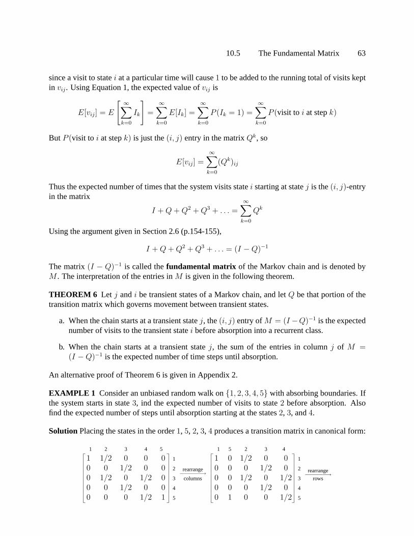
EXAMPLE 3 Consider an unbiased random walk on{1, 2, 3, 4, 5} with absorbing boundaries.The transition matrix is

P =

1 2 3 4 5

1 1/2 0 0 0 1

0 0 1/2 0 0 2

0 1/2 0 1/2 0 3

0 0 1/2 0 0 4

0 0 0 1/2 1 5


Notice that only two long-term possibilities exist for this chain – it must end up in state0 or state4.Thus the probability that the chain is in states1, 2 or 3 becomes smaller and smaller asn increases,asP n illustrates:

P 20 =

1 .74951 .49951 .24951 00 .00049 0 .00049 00 0 .00098 0 00 .00049 0 .00049 00 .24951 .49951 .74951 1

, P 30 =

1 .749985 .499985 .249985 00 .000015 0 .000015 00 0 .000030 0 00 .000015 0 .000015 00 .249985 .499985 .749985 1

It seems thatP n converges to the matrix

1 .75 .5 .25 00 0 0 0 00 0 0 0 00 0 0 0 00 .25 .5 .75 1

asn increases. But the columns of this matrix are not equal; the probability of ending up eitherat 1 or at5 depends on where the chain begins. Although the chain has steady-state vectors, theycannot be interpreted as in Example 1. Exercise 23 confirms that if0 ≤ q ≤ 1 the vector

q000

1− q

is a steady-state vector forP . This matrix then has an infinite number of possible steady-statevectors, which shows in another way thatxn cannot be expected to have convergent behaviorwhich does not depend onx0. �

EXAMPLE 4 Consider an unbiased random walk on{1, 2, 3, 4, 5} with reflecting boundaries.The transition matrix is

P =

1 2 3 4 5

0 1/2 0 0 0 1

1 0 1/2 0 0 2

0 1/2 0 1/2 0 3

0 0 1/2 0 1 4

0 0 0 1/2 0 5

If the chainxn starts at state1, notice that it can return to1 only whenn is even, while the chaincan be at state2 only whenn is odd. In fact, the chain must be at an even-numbered site whenn isodd and at an odd-numbered site whenn is even. If the chain were to start at state2, however, thissituation would be reversed: the chain must be at an odd-numbered site whenn is odd and at an


even-numbered site whenn is even. Therefore,P n cannot converge to a unique matrix sinceP n

looks very different depending on whethern is even or odd, as shown:

P 20 =

.2505 0 .2500 0 .2495

0 .5005 0 .4995 0.5000 0 .5000 0 .5000

0 .4995 0 .5005 0.2495 0 .2500 0 .2505

, P 21 =

0 .2502 0 .2498 0

.5005 0 .5000 0 .49950 .5000 0 .5000 0

.4995 0 .5000 0 .50050 .2498 0 .2502 0

Even thoughP n does not converge to a unique matrix,P does have a steady-state vector. In fact,

1/81/41/41/41/8

is a steady-state vector forP (see Exercise 32). This vectorcan be interpreted as giving long-runprobabilities and occupation times in a sense that will be made precise in Section 10.4. �

EXAMPLE 5 Consider a Markov chain on{1, 2, 3, 4, 5} with transition matrix

P =

1 2 3 4 5

1/4 1/3 1/2 0 0 1

1/4 1/3 1/4 0 0 2

1/2 1/3 1/4 0 0 3

0 0 0 1/3 3/4 4

0 0 0 2/3 1/4 5

If this Markov chain begins in states1, 2, or 3, then it must always be at one of those states.Likewise if the chain starts at states4 or 5, then it must always be at one of those states. The chainsplits into two separate chains, each with its own steady-state vector. In this caseP n converges toa matrix whose columns are not equal. The vectors

4/113/114/11

00

and

000

9/178/17

both satisfy the definition of steady-state vector (Exercise 33). The first vector gives the limitingprobabilities if the chain starts at states1, 2, or 3, and the second does the same for the states4 and5. �


Regular Matrices

Examples 1 and 2 show that in some cases a Markov chainxn with transition matrixP has asteady-state vectorq for which

limn→∞

P n =[

q q · · · q]

In these cases,q can be interpreted as a vector of long-run probabilities or occupation times for thechain. These probabilities or occupation times do not depend on the initial probability vector; thatis, for any probability vectorx0,

limn→∞

P nx0 = limn→∞

xn = q

Notice also thatq is the only probability vector which is also an eigenvector ofP associated withthe eigenvalue1.

Examples 3, 4, and 5 do not have such a steady-state vectorq. In Examples 3 and 5 the steady-state vector is not unique; in all three examples the matrixP n does not converge to a matrix withequal columns asn increases. The goal is then to find some property of the transition matrixP thatleads to these different behaviors, and to show that this property causes the differences in behavior.

A little calculation shows that in Examples 3, 4, and 5, every matrix of the formP k has somezero entries. In Examples 1 and 2, however, some power ofP has all positive entries. As wasmentioned in Section 4.9, this is exactly the property that is needed.

DEFINITION A stochastic matrixP is regular if some powerP k contains only strictly positiveentries.

Since the matrixP k contains the probabilities of ak-step move from one state to another, aMarkov chain with a regular transition matrix has the property that, for somek, it is possible tomove from any state to any other in exactlyk steps. The following theorem expands upon thecontent of Theorem 18 in Section 4.9. One idea must be defined before the theorem is presented.The limit of a sequence ofm × n matrices is them × n matrix (if one exists) whose(i, j) entryis the limit of the(i, j) entries in the sequence of matrices. With that understanding, here is thetheorem.

THEOREM 1 If P is a regularm×m transition matrix withm ≥ 2, then the following statementsare all true.

(a) There is a stochastic matrixΠ such thatlimn→∞

P n = Π.

(b) Each column ofΠ is the same probability vectorq.

(c) For any initial probability vectorx0, limn→∞

P nx0 = q.

(d) The vectorq is the unique probability vector which is an eigenvector ofP associated withthe eigenvalue1.

(e) All eigenvaluesλ of P other than1 have|λ| < 1.


A proof of Theorem 1 is given in Appendix 1. Theorem 1 is a special case of the Perron-Frobenius Theorem, which is used in applications of linear algebra to economics, graph theory,and systems analysis. Theorem 1 shows that a Markov chain with a regular transition matrix hasthe properties found in Examples 1 and 2. For example, since the transition matrixP in Example 1is regular, Theorem 1 justifies the conclusion thatP n converges to a stochastic matrix all of whose

columns equalq =

.3.6.1

, as numerical evidence seemed to indicate.

PageRank and the Google Matrix

In Section 1, the notion of a simple random walk on a graph was defined. The World Wide Webcan be modeled as a directed graph, with the vertices representing the webpages and the arrowsrepresenting the links between webpages. LetP be the huge transition matrix for this Markovchain. If the matrixP were regular, then Theorem 1 would show that there is a steady-state vectorq for the chain, and that the entries inq can be interpreted as occupation times for each state.In terms of the model, the entries inq would tell what fraction of the random surfer’s time wasspent at each webpage. The founders of Google, Sergey Brin and Lawrence Page, reasoned that“important” pages had links coming from other “important” pages. Thus the random surfer wouldspend more time at more important pages and less time at less important pages. But the amountof time spent at each page is just the occupation time for each state in the Markov chain. Thisobservation is the basis for PageRank, which is the model that Google uses to rank the importanceof all webpages it catalogs:

The importance of a webpage may be measured by the rela-tive size of the corresponding entry in the steady-state vectorq for an appropriately chosen Markov chain.

Unfortunately, simple random walk on the directed graph model for the Web is not the appro-priate Markov chain, because the matrixP is not regular. Thus Theorem 1 will not apply. Forexample, consider the seven-page Web modeled in Section 10.1 using the directed graph in Figure1. The transition matrix is

P =

1 2 3 4 5 6 7

0 1/2 0 0 0 0 0 1

0 0 1/3 0 1/2 0 0 2

1 0 0 0 0 1/3 0 3

0 0 1/3 1 0 0 0 4

0 1/2 0 0 0 1/3 0 5

0 0 1/3 0 1/2 0 0 6

0 0 0 0 0 1/3 1 7

Pages4 and7 are dangling nodes, and so are absorbing states for the chain. Just as in Example 3,the presence of absorbing states implies that the state vectorsxn do not approach a unique limit asn→∞. To handle dangling nodes, an adjustment is made toP :


1

2

3

4

5 6

7

Figure 1: A seven-page Web.

ADJUSTMENT 1: If the surfer reaches a dangling node, the surfer will pick any page in the Webwith equal probability and will move to that page. In terms of the transition matrixP , if statej isan absorbing state, replace columnj of P with the vector

1/n1/n

...1/n

wheren is the number of rows (and columns inP ).In the seven-page example, the transition matrix is now

P∗ =

1 2 3 4 5 6 7

0 1/2 0 1/7 0 0 1/7 1

0 0 1/3 1/7 1/2 0 1/7 2

1 0 0 1/7 0 1/3 1/7 3

0 0 1/3 1/7 0 0 1/7 4

0 1/2 0 1/7 0 1/3 1/7 5

0 0 1/3 1/7 1/2 0 1/7 6

0 0 0 1/7 0 1/3 1/7 7

Yet even this adjustment is not sufficient to ensure that the transition matrix is regular: whiledangling nodes are no longer possible, it is still possible to have “cycles” of pages. If pagej linkedonly to pagei and pagei linked only to pagej, a random surfer entering either page would becondemned to spend eternity linking from pagei to pagej and back again. Thus the columns ofP k∗ corresponding to these pages would always have zeros in them, and the transition matrixP∗

would not be regular. Another adjustment is needed.

ADJUSTMENT 2: Let p be a number between0 and1. Assume the surfer is now at pagej.With probabilityp the surfer will pick from among all possible links from the pagej with equalprobability and will move to that page. With probability1− p the surfer will pickanypage in the


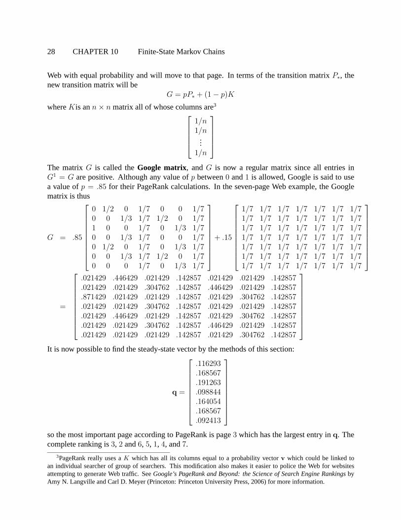
Web with equal probability and will move to that page. In terms of the transition matrixP∗, thenew transition matrix will be

G = pP∗ + (1− p)K

whereK is ann× n matrix all of whose columns are31/n1/n

...1/n

The matrixG is called theGoogle matrix, andG is now a regular matrix since all entries inG1 = G are positive. Although any value ofp between0 and1 is allowed, Google is said to usea value ofp = .85 for their PageRank calculations. In the seven-page Web example, the Googlematrix is thus

G = .85

0 1/2 0 1/7 0 0 1/70 0 1/3 1/7 1/2 0 1/71 0 0 1/7 0 1/3 1/70 0 1/3 1/7 0 0 1/70 1/2 0 1/7 0 1/3 1/70 0 1/3 1/7 1/2 0 1/70 0 0 1/7 0 1/3 1/7

+ .15

1/7 1/7 1/7 1/7 1/7 1/7 1/71/7 1/7 1/7 1/7 1/7 1/7 1/71/7 1/7 1/7 1/7 1/7 1/7 1/71/7 1/7 1/7 1/7 1/7 1/7 1/71/7 1/7 1/7 1/7 1/7 1/7 1/71/7 1/7 1/7 1/7 1/7 1/7 1/71/7 1/7 1/7 1/7 1/7 1/7 1/7

=

.021429 .446429 .021429 .142857 .021429 .021429 .142857

.021429 .021429 .304762 .142857 .446429 .021429 .142857

.871429 .021429 .021429 .142857 .021429 .304762 .142857

.021429 .021429 .304762 .142857 .021429 .021429 .142857

.021429 .446429 .021429 .142857 .021429 .304762 .142857

.021429 .021429 .304762 .142857 .446429 .021429 .142857

.021429 .021429 .021429 .142857 .021429 .304762 .142857

It is now possible to find the steady-state vector by the methods of this section:

q =

.116293

.168567

.191263

.098844

.164054

.168567

.092413

so the most important page according to PageRank is page3 which has the largest entry inq. Thecomplete ranking is3, 2 and6, 5, 1, 4, and7.

3PageRank really uses aK which has all its columns equal to a probability vectorv which could be linked toan individual searcher of group of searchers. This modification also makes it easier to police the Web for websitesattempting to generate Web traffic. SeeGoogle’s PageRank and Beyond: the Science of Search Engine RankingsbyAmy N. Langville and Carl D. Meyer (Princeton: Princeton University Press, 2006) for more information.


NUMERICAL NOTEThe computation ofq is not a trivial task, since the Google matrix has over 8 billion rows andcolumns. Google uses a version of the power method introduced in Section 5.8 to computeq.While the power method was used in that section to estimate the eigenvalues of a matrix, it canalso be used to provide estimates for eigenvectors. Sinceq is an eigenvector ofG correspondingto the eigenvalue1, the power method applies. It turns out that only between 50 and 100 iterationsof the method are needed to get the vectorq to the accuracy that Google needs for its rankings. Itstill takes days for Google to compute a newq, which it does every month.

Practice Problem

1. Consider the Markov chain on{1, 2, 3} with transition matrix

P =

1/2 0 1/21/2 1/2 0

0 1/2 1/2

a. Show thatP is a regular matrix.

b. Find the steady-state vector for this Markov chain.

c. What fraction of the time does this chain spend in state 2? Explain your answer.


10.2 ExercisesIn Exercises 1 and 2, consider a Markov chainon {1, 2} with the given transition matrixP . Ineach exercise, use two methods to find the prob-ability that, in the long run, the chain is in state1. First, raiseP to a high power. Then directlycompute the steady-state vector.

1. P =

[.2 .4.8 .6

]

2. P =

[.95 .05.05 .95

]In Exercises 3 and 4, consider a Markov chainon {1, 2, 3} with the given transition matrixP .In each exercise, use two methods to find theprobability that, in the long run, the chain is instate 1. First, raiseP to a high power. Thendirectly compute the steady-state vector.

3. P =

1/3 1/4 01/3 1/2 11/3 1/4 0

4. P =

.1 .2 .3.2 .3 .4.7 .5 .3

In Exercises 5 and 6, find the matrix to whichP n converges asn increases.

5. P =

[1/4 2/33/4 1/3

]

6. P =

1/4 3/5 01/4 0 1/31/2 2/5 2/3

In Exercises 7 and 8, determine whether the givenmatrix is regular. Explain your answer.

7. P =

1/3 0 1/21/3 1/2 1/21/3 1/2 0

8. P =

1/2 0 1/3 00 2/5 0 3/71/2 0 2/3 00 3/5 0 4/7

9. Consider a pair of Ehrenfest urns with a

total of8 molecules divided between them.

a. Find the transition matrix for the Mar-kov chain which models the numberof molecules in UrnA, and show thatthis matrix is not regular.

b. Assuming that the steady-state vec-tor may be interpreted as occupationtimes for this Markov chain, in whatstate will this chain spend the moststeps?

10. Consider a pair of Ehrenfest urns with atotal of7 molecules divided between them.

a. Find the transition matrix for the Mar-kov chain which models the numberof molecules in UrnA, and show thatthis matrix is not regular.


11. Consider unbiased random walk with re-flecting boundaries on{1, 2, 3, 4, 5, 6}.

a. Find the transition matrix for the Mar-kov chain and show that this matrixis not regular.



12. Consider biased random walk with reflect-ing boundaries on{1, 2, 3, 4, 5, 6}with p =2/3.

a. Find the transition matrix for the Mar-kov chain and show that this matrixis not regular.


In Exercises 13 and 14, consider a simple ran-dom walk on the graph given. In the long run,what fraction of the time is the walk at the vari-ous states?

13.1 2

34

5

14.1 2

34

In Exercises 15 and 16, consider a simple ran-dom walk on the directed graph given. In thelong run, what fraction of the time is the walk atthe various states?

15.1 2

3 4

16.1

2

3

4

5

17. Consider the mouse in the following mazefrom Section 1, Exercise 17.

1 2

3

4 5

The mouse must move into a differentroom at each time step, and is equallylikely to leave the room through any of theavailable doorways. If you go away fromthe maze for a while, what is the probabil-ity that the mouse is in room 3 when youreturn?


1 2 3

4 5


What fraction of time does it spend inroom 3?

19. Consider the mouse in the following mazethat includes “one-way” doors from Sec-tion 1, Exercise 19.

1 2 3

4 5 6

Show that

q =

000001

is a steady-state vector for the associatedMarkov chain, and interpret this result interms of the mouse’s travels through themaze.

20. Consider the mouse in the following mazethat includes “one-way” doors.

1 2

3

4 5

What fraction of time does it spend in eachof the rooms in the maze?


21. a. Every stochastic matrix has a steady-state vector.

b. If its transition matrix is regular, thenthe steady-state vector gives informa-tion on long-run probabilities of theMarkov chain.

c. If λ = 1 is an eigenvalue of a matrixP , thenP is regular.

22. a. Every stochastic matrix is regular.

b. If P is a regular stochastic matrix,then P n approaches a matrix withequal columns asn increases.

c. If limn→∞

xn = q, then the entries in

q may be interpreted as occupationtimes.

23. Suppose that the weather in Charlotte ismodeled using the Markov chain in Sec-tion 1, Exercise 17. Over the course of ayear, about how many days in Charlotteare sunny, cloudy, and rainy according tothe model?

24. Suppose that the weather in Charlotte ismodeled using the Markov chain in Sec-tion 1, Exercise 18. Over the course of ayear, about how many days in Charlotteare rainy according to the model?

In Exercises 25 and 26, consider a set of web-pages hyperlinked by the given directed graph.Find the Google matrix for each graph and com-pute the PageRank of each page in the set.

25.1 2

3 4

5


26.

1

2

3

4

5 6

27. A genetic trait is often governed by a pairof genes, one inherited from each parent.The genes may be of two types, often la-belled A and a. An individual then mayhave three different pairs: AA, Aa (whichis the same as aA), or aa. In many casesthe AA and Aa individuals cannot be oth-erwise distinguished – in these cases geneA is dominantand gene a isrecessive.Likewise an AA individual is calleddom-inant and an aa individual is calledreces-sive. An Aa individual is called ahybrid.

a. Show that if a dominant individualis mated with a hybrid, the proba-bility of an offspring being dominantis 1/2 and the probability of an off-spring being a hybrid is1/2.

b. Show that if a recessive individual ismated with a hybrid, the probabilityof an offspring being recessive is1/2and the probability of an offspringbeing a hybrid is1/2.

c. Show that if a hybrid individual ismated with a hybrid, the probabil-ity of an offspring being dominant is1/4, the probability of an offspringbeing recessive is1/4, and the prob-ability of an offspring being a hybridis 1/2.

28. Consider beginning with an individual ofknown type and mating it with a hybrid,then mating an offspring of this mating

with a hybrid, and so on. At each stepan offspring is mated with a hybrid. Thetype of the offspring can be modelled by aMarkov chain with states AA, Aa, and aa.

a. Find the transition matrix for this Mar-kov chain.

b. If the mating process of the previousExercise is continued for a extendedperiod of time, what percent of theoffspring are of each type?

29. Consider the variation of the Ehrenfest urnmodel of diffusion studied in Section 1,Exercise 29, where one of the2k moleculesis chosen at random and is then moved be-tween the urns with a fixed probabilityp.

a. Let k = 3 and suppose thatp =1/2. Show that the transition ma-trix for the Markov chain that mod-els the number of molecules in UrnA is regular.

b. Letk = 3 and suppose thatp = 1/2.In what state will this chain spendthe most steps, and what fraction ofthe steps will the chain spend at thisstate?

c. Does the answer to part b. change ifa different value ofp with 0 < p < 1is used?

30. Consider the Bernoulli-Laplace of diffu-sion studied in Section 1, Exercise 30.

a. Letk = 5 and show that the transi-tion matrix for the Markov chain thatmodels the number of Type I moleculesin Urn A is regular.

b. Let k = 5. In what state will thischain spend the most steps, and whatfraction of the steps will the chainspend at this state?


31. Let0 ≤ q ≤ 1. Show that

q000

1− q

is

a steady-state vector for the Markov chainin Example 3.

32. Consider the Markov chain in Example 4.

a. Show that

1/81/41/41/41/8

is a steady-state

vector for this Markov chain.

b. Compute the average of the entriesin P 20 andP 21 given in Example 4.What do you find?

33. Show that

4/113/114/11

00

and

000

9/178/17

are

steady-state vectors for the Markov chainin Example 5. If the chain is equally likelyto begin in each of the states, what is theprobability of being in state 1 after manysteps?

34. Let0 ≤ p, q ≤ 1, and define

P =

[p 1− q

1− p q

]a. Show that1 andp + q− 1 are eigen-

values ofP .

b. By Theorem 1, for what values ofpandq will P fail to be regular?

c. Find a steady-state vector forP .

35. Let0 ≤ p, q ≤ 1, and define

P=

p q 1− p− qq 1− p− q p

1− p− q p q

a. For what values ofp and q is P aregular stochastic matrix?

b. Given thatP is regular, find a steady-state vector forP .

36. LetA be anm ×m non-negative matrix,x be inRm, andy = Ax. Show that

|y1|+ . . . + |ym| ≤ |x1|+ . . . + |xm|

with equality holding if and only if all ofthe nonzero entries inx have the same sign.

37. Show that every stochastic matrix has asteady-state vector using the followingsteps.

a. LetP be a stochastic matrix. By Ex-ercise 30 in Section 4.9,λ = 1 is aneigenvalue forP . Letv be an eigen-vector ofP associated withλ = 1.Use Exercise 36 to conclude that thenonzero entries inv must have thesame sign.

b. Show how to produce a steady-statevector forP from v.

38. Consider simple random walk on a finiteconnected graph. (A graph is connected ifit is possible to move from any vertex ofthe graph to any other along the edges ofthe graph).

a. Explain why this Markov chain musthave a regular transition matrix.

b. Use the results of Exercises 13 and14 to hypothesize a formula for thesteady-state vector for such a Markovchain.

39. By Theorem 1 (e) all eigenvaluesλ of aregular matrix other than1 have the prop-erty that|λ| < 1; that is, the eigenvalue1 is a strictly dominant eigenvalue. Sup-pose thatP is ann×n regular matrix with


eigenvaluesλ1 = 1, . . . , λn ordered sothat |λ1| > |λ2| ≥ |λ3| ≥ . . . ≥ |λn|.Suppose thatx0 is a linear combination ofeigenvectors ofP .

a. Use Equation (2) in Section 5.8 toderive an expression forxk = P kx0.

b. Use the result of part (a) to derivean expression forxk − q, and ex-plain how the value of|λ2| effectsthe speed with which{xk} convergesto q.


Solutions to Practice Problem

1. a. Since

P 2 =

1/4 1/4 1/21/2 1/4 1/41/4 1/2 1/4

P is regular by the definition withk = 2.

b. Solve the equationPq = q, which may be re-written as(P − I)q = 0. Since

P − I =

−1/2 0 1/21/2 −1/2 00 1/2 −1/2

Row reducing the augmented matrix gives −1/2 0 1/2 0

1/2 −1/2 0 00 1/2 −1/2 0

∼ 1 0 −1 0

0 1 −1 00 0 0 0

so the general solution isq3

111

. Sinceq must be a probability vector, setq3 =

1/(1 + 1 + 1) = 1/3 and compute that

q =1

3

111

=

1/31/31/3

c. The chain will spend1/3 of its time in state 2 since the entry inq corresponding to

state 2 is1/3, and we can interpret the entries as occupation times.

10.3 Communication Classes 37

10.3 Communication Classes

Section 10.2 showed that if the transition matrix for a Markov chain is regular, thenxn convergesto a unique steady-state vector for any choice of initial probability vector. That is,lim

n→∞xn = q,

whereq is the unique steady-state vector for the Markov chain. Examples 3, 4, and 5 of Section10.2 illustrated that, even though every Markov chain has a steady-state vector, not every Markovchain has the property thatlim

n→∞xn = q. The goal of the next two sections is to study these

examples further, and to show that Examples 3, 4, and 5 of Section 10.2 describe all the ways inwhich Markov chains fail to converge to a steady-state vector. The first step is to study which statesof the Markov chain can be reached from other states of the chain.

Communicating States

Suppose that statej and statei are two states of a Markov chain. If the statej can be reachedfrom the statei in a finite number of steps and the statei can be reached from the statej in a finitenumber of steps, then the statesj andi are said tocommunicate. If P is the transition matrix forthe chain, then the entries inP k give the probabilities of going from one state to another ink steps:

P k =

From:1 j m To:

... 1

↓pij · · · → i

m

and powers ofP can be used to make the following definition.

DEFINITION Let i andj be two states of a Markov chain with transition matrixP . Then stateicommunicateswith statej if there exist nonnegative integersm andn such that the(j, i) entry ofPm and the(i, j) entry ofP n are both strictly positive. That is, statei communicates with statejif it is possible to go from statei to statej in m steps and from statej to statei in n steps.

This definition implies three properties that will allow the states of a Markov chain to be placedinto groups calledcommunication classes. First, the definition allows the integersm andn to bezero, in which case the(i, i) entry ofP 0 = I is 1, which is positive. This insures that every statecommunicates with itself. Because both(i, j) and(j, i) are included in the definition, it followsthat if statei communicates with statej then statej communicates with statei. Finally, you willshow in Exercise 36 that if statei communicates with statej and statej communicates with statek,then statei communicates with statek. These three properties are called respectively thereflexive,symmetric, andtransitive properties:

(a) (Reflexive Property) Each state communicates with itself.

(b) (Symmetric Property) If statei communicates with statej, then statej communicates withstatei.


(c) (Transitive Property) If statei communicates with statej, and statej communicates withstatek, then statei communicates with statek.

A relation with these three properties is called anequivalence relation. The communication rela-tion is an equivalence relation on the state space for the Markov chain. Using the properties listedabove simplifies determining which states communicate.

EXAMPLE 1 Consider an unbiased random walk with absorbing boundaries on{1, 2, 3, 4, 5}.Find which states communicate.

Solution The transition matrixP is given below along with the transition diagram for this Markovchain:

P =

1 2 3 4 5

1 1/2 0 0 0 1

0 0 1/2 0 0 2

0 1/2 0 1/2 0 3

0 0 1/2 0 0 4

0 0 0 1/2 1 5

1

2

1

2

1

2

1

2

1

2

1

2

1 2 3 4 51 1

Figure 1: Unbiased random walk with absorbing boundaries.

First note by the reflexive property each state communicates with itself. It is clear from the diagramthat states2, 3 and4 communicate with each other. The same conclusion may be reached using thedefinition by finding that the(2, 3), (3, 2), (3, 4), and(4, 3) entries inP are positive, thus states2and3 communicate, as do states3 and4. States2 and4 must also communicate by the transitiveproperty. Now consider state1 and state5. If the chain starts in state1, it cannot move to any stateother than itself. Thus it is not possible to go from state1 to any other state in any number of steps,and state1 does not communicate with any other state. Likewise state5 does not communicatewith any other state. In summary,

State1 communicates with state1.State2 communicates with state2, state3, and state4.State3 communicates with state2, state3, and state4.State4 communicates with state2, state3, and state4.State5 communicates with state5.


Notice that even though the states1 and5 do not communicate with states2, 3 and4, it is possibleto go from these states either state1 or state5 in a finite number of steps: this is clear from thediagram, or by confirming that the appropriate entries inP , P 2, or P 3 are positive. �

In Example 1 the state space{1, 2, 3, 4, 5} can now be divided into the classes{1}, {2, 3, 4},and{5}. The states in each of these classes communicate only with the other members of theirclass. This division of the state space occurs because the communication relation is an equivalencerelation. The communication relationpartitions the state space intocommunication classes. Eachstate in a Markov chain communicates only with the members of its communication class. For theMarkov chain in Example 1, the communication classes are{1}, {2, 3, 4}, and{5}.

EXAMPLE 2 Consider an unbiased random walk with reflecting boundaries on{1, 2, 3, 4, 5}.Find the communication classes for this Markov chain.

Solution The transition matrixP for this chain, as well asP 2, P 3, andP 4, are shown below.

P =

1 2 3 4 5

0 1/2 0 0 0 1

1 0 1/2 0 0 2

0 1/2 0 1/2 0 3

0 0 1/2 0 1 4

0 0 0 1/2 0 5

, P 2 =

1 2 3 4 5

1/2 0 1/4 0 0 1

0 3/4 0 1/4 0 2

1/2 0 1/2 0 1/2 3

0 1/4 0 3/4 0 4

0 0 1/4 0 1/2 5

P 3 =

1 2 3 4 5

0 3/8 0 1/8 0 1

3/4 0 1/2 0 1/4 2

0 1/2 0 1/2 0 3

1/4 0 1/2 0 3/4 4

0 1/8 0 3/8 0 5

, P 4 =

1 2 3 4 5

3/8 0 1/4 0 1/8 1

0 5/8 0 3/8 0 2

1/2 0 1/2 0 1/2 3

0 3/8 0 5/8 0 4

1/8 0 1/4 0 3/8 5

The transition diagram for this Markov chain is given in Figure 2.

1

1

2

1

2

1

2

1

2

1

2

1

2

1

1 2 3 4 5

Figure 2: Unbiased random walk with reflecting boundaries.

Notice that the(i, j) entry in at least one of these matrices is positive for any choice ofi andj.Thus every state is reachable from any other state in4 steps or fewer, and every state communicateswith every state. There is only one communication class:{1, 2, 3, 4, 5}. �


EXAMPLE 3 Consider the Markov chain given in Example 5 of Section 10.2. Find the commu-nication classes for this Markov chain.

Solution The transition matrix for this Markov chain is

P =

1 2 3 4 5

1/4 1/3 1/2 0 0 1

1/4 1/3 1/4 0 0 2

1/2 1/3 1/4 0 0 3

0 0 0 1/3 3/4 4

0 0 0 2/3 1/4 5

and a transition diagram is

1

4

1

3

2

3

1

2

1

3

1

4

3

4

1

2

1

2

3 4 5

1

4

1

3 1

4

1

3

1

4

Figure 3: Transition diagram for Example 3.

It is impossible to move from any of the states1, 2, or3 to either of the states4 or 5, so these statesmust be in separate communication classes. In addition, state1, state2, and state3 communicate;state4 and state5 also communicate. Thus the communication classes for this Markov chain are{1, 2, 3} and{4, 5}. �

The Markov chains in Examples 1 and 3 have more than one communication class, whilethe Markov chain in Example 2 has only one communication class. This distinction leads to thefollowing definitions.

DEFINITION A Markov chain with only one communication class isirreducible . A Markovchain with more than one communication class isreducible.


Thus the Markov chains in Examples 1 and 3 are reducible, while the Markov chain in Example2 is irreducible. Irreducible Markov chains and regular transition matrices are connected by thefollowing theorem.

THEOREM 2 If a Markov chain has a regular transition matrix, then it is irreducible.

Proof Suppose thatP is a regular transition matrix for a Markov chain. Then by definition, thereis ak such thatP k is a positive matrix. That is, for any statesi andj, the(i, j) and(j, i) elementsin P k are strictly positive. Thus there is a positive probability of moving fromi to j and fromjto i in exactlyk steps, and soi andj communicate with each other. Sincei andj are any statesand must be in the same communication class, there can be only one communication class for thechain, so the Markov chain must be irreducible. �

Example 2 shows that the converse of Theorem 2 is not true, because the Markov chain in thisexample is irreducible, but its transition matrix is not regular.

EXAMPLE 4 Consider the Markov chain whose transition diagram is given in Figure 4. Deter-mine whether this Markov chain is reducible or irreducible.

.2 .4

1

.3 .1

1

.6

.8 .6

1

2

3

4

5


Solution The diagram shows that states1 and2 communicate, as do states4 and5. Notice thatstates1 and2 cannot communicate with states3, 4, or 5 since the probability of moving fromstate2 to state3 is 0. Likewise states4 and5 cannot communicate with states1, 2, or 3 sincethe probability of moving from state4 to state3 is 0. Finally, state3 cannot communicate withany state other than itself since it is impossible to return to state3 from any other state. Thus thecommunication classes for this Markov chain are{1, 2}, {3}, and{4, 5}. Since there is more thanone communication class, this Markov chain is reducible. �


Mean Return Times

Let q be the steady-state vector for an irreducible Markov chain. It can be shown using advancedmethods in probability theory that the entries inq may be interpreted as occupation times; that is,qi is the fraction of time steps that the chain will spend at statei. For example, consider a Markov

chain on{1, 2, 3} with steady-state vectorq =

.2.5.3

. In the long run the chain will spend about

half of its steps in state2. If the chain is currently at state2, it should take about2 = 1/.5 stepsto return to state2. Likewise since the chain spends about1/5 of its time in state1, it should visitstate1 once every5 steps.

Given a Markov chain and statesi andj, a quantity of considerable interest is the number ofstepsnij that it will take for the system to first visit statei given that it is started in statej. Thevalue ofnij cannot be known – it could be any positive integer depending on how the Markovchain evolves. Such a quantity is known as arandom variable. Sincenij is unknowable, theexpected valueof nij is studied instead. The expected value of a random variable functions as atype of average value of the random variable. The following definition will be used in subsequentsections.

DEFINITION Theexpected value of a random variableX which takes on the valuesx1, x2, . . .is

E[X] = x1P (X = x1) + x2P (X = x2) + · · · =∞∑

k=1

xkP (X = xk) (1)

whereP (X = xk) denotes the probability that the random variableX equals the valuexk.

Now let tii = E[nii] be the expected value ofnii, which is the expected number of steps it willtake for the system to return to statei given that it starts in statei. Unfortunately, Equation 1 willnot be helpful at this point. Instead proceeding intuitively, the system should spend1 step at statei for eachtii steps on average. It seems reasonable to say that the system will, over the long run,spend about1/tii of the time at statei. But that quantity isqi, so the expected time steps neededto return, ormean return time to a statei, is the reciprocal ofqi. This informal argument may bemade rigorous using methods from probability theory; see Appendix 2 for a complete proof.

THEOREM 3 Consider an irreducible Markov chain with a finite state space, letnij be the num-ber of steps until the chain first visits statei given that the chain starts in statej, and lettii = E[nii].Then

tii =1

qi

(2)

whereqi is the entry in the steady-state vectorq corresponding to statei.

The above example matches Equation 2:t11 = 1/.2 = 5, t22 = 1/.5 = 2, andt33 = 1/.3 = 10/3.Recall that the mean return time is a expected value, so the fact thatt33 is not an integer ought notbe troubling. Section 10.5 will include a discussion oftij = E[nij] wherei 6= j.


Practice Problem

1. Consider the Markov chain on{1, 2, 3, 4} with transition matrix

P =

1/4 1/3 1/2 00 1/3 0 1/3

3/4 0 1/2 1/30 1/3 0 1/3

Determine the communication classes for this chain.


10.3 ExercisesIn Exercises 1-6, consider a Markov chain withstate space with{1, 2, . . . , n} and the given tran-sition matrix. Find the communication classesfor each Markov chain, and state whether theMarkov chain is reducible or irreducible.

1.

1/4 0 1/31/2 1 01/4 0 1/3

2.

1/4 1/2 1/31/2 1/2 01/4 0 1/3

3.

1 1/2 1/20 1/2 00 0 1/2

4.

0 0 0 1 1

1/3 0 0 0 02/3 0 0 0 00 1/4 2/3 0 00 3/4 1/3 0 0

5.

0 0 .4 0 .8 00 0 0 .7 0 .5.3 0 0 0 .2 00 .1 0 0 0 .5.7 0 .6 0 0 00 .9 0 .3 0 0

6.

0 1/3 0 2/3 1/2 0 01/2 0 1/2 0 0 1/3 00 2/3 0 1/3 0 0 2/5

1/2 0 1/2 0 0 0 00 0 0 0 0 0 3/50 0 0 0 1/2 0 00 0 0 0 0 2/3 0


1 2 3

4 5 6

Find the communication classes for theMarkov chain that models the mouse’s trav-els through this maze. Is this Markov chainreducible or irreducible?


1 2

3

4 5

Find the communication classes for theMarkov chain that models the mouse’s trav-els through this maze. Is this Markov chainreducible or irreducible?

In Exercises 9 and 10, consider the set of web-pages hyperlinked by the given directed graph.Find the communication classes for the Markovchain that models a random surfer’s prog-ress through this set of webpages.


9.1 2

3 4

5

10.1

2

3

4

5 6

11. Consider unbiased random walk withreflecting boundaries on{1, 2, 3, 4, 5, 6}.Find the communication classes for thisMarkov chain and determine whether it isreducible or irreducible.

12. Consider unbiased random walk withabsorbing boundaries on{1, 2, 3, 4, 5, 6}.Find the communication classes for thisMarkov chain and determine whether it isreducible or irreducible.

In Exercises 13 and 14, consider a simple ran-dom walk on the graph given. Show that theMarkov chain is irreducible and calculate themean return times for each state.

13.1 2

34

5

14.1 2

34

In Exercises 15 and 16, consider a simple ran-dom walk on the directed graph given. Showthat the Markov chain is irreducible and calcu-late the mean return times for each state.

15.1 2

3 4

16.1

2

3

4

5


1 2

3

4 5


If the mouse starts in room 3, how long onaverage will it take the mouse to return toroom 3?


1 2 3

4 5

If the mouse starts in room 2, how long onaverage will it take the mouse to return toroom 2?

In Exercises 19 and 20, consider the mouse inthe following maze from Section 2, Exercise 20.

1 2

3

4 5

19. If the mouse starts in room 1, how long onaverage will it take the mouse to return toroom 1?

20. If the mouse starts in room 4, how long onaverage will it take the mouse to return toroom 4?


21. a. If it is possible to go from stateito statej in n steps, wheren ≥ 0,then statesi andj communicate witheach other.

b. If a Markov chain is reducible, thenit cannot have a regular transition ma-trix.

c. The entries in the steady-state vectorare the mean return times for eachstate.

22. a. An irreducible Markov chain musthave a regular transition matrix.

b. If the (i, j) and (j, i) entries inP k

are positive for somek, then the statesi andj communicate with each other.

c. If statei communicates with statejand statej communicates with statek, then statei communicates with statek.

23. Suppose that the weather in Charlotte ismodeled using the Markov chain in Sec-tion 1, Exercise 23. About how many dayselapse in Charlotte between rainy days?

24. Suppose that the weather in Charlotte ismodeled using the Markov chain in Sec-tion 1, Exercise 24. About how many dayselapse in Charlotte between consecutiverainy days?

25. The following set of web pages hyperlinkedby the directed graph was studied in Sec-tion 2, Exercise 25.

1 2

3 4

5

Consider randomly surfing on this set ofweb pages using the Google matrix as thetransition matrix.

a. Show that this Markov chain is irre-ducible.


b. Suppose the surfer starts at page 1.How many mouse clicks on averagemust the surfer make to get back topage 1?

26. The following set of web pages hyperlinkedby the directed graph that was studied inSection 2, Exercise 26.

1

2

3

4

5 6

Repeat Exercise 25 for this set of web pages.

27. Consider the pair of Ehrenfest urns stud-ied in Section 2, Exercise 9. Suppose thatthere are now 4 molecules in UrnA. Howmany steps on average will be needed un-til there are again 4 molecules in UrnA?

28. Consider the pair of Ehrenfest urns stud-ied in Section 2, Exercise 10. Supposethat UrnA is now empty. How many stepson average will be needed until UrnA isagain empty?

29. A variation of the Ehrenfest model of dif-fusion studied in Section 2, Exercise 29.Consider this model withk = 3 andp =1/2 and suppose that there are now 3 mole-cules in UrnA. How many draws on av-erage will be needed until there are again3 molecules in UrnA?

30. Consider the Bernoulli-Laplace model ofdiffusion studied in Section 2, Exercise 30.Let k = 5. Suppose that all of the Type Imolecules are now in UrnA. How manydraws on average will be needed until allof the Type I molecules are again in UrnA?

31. A Markov chain model for scoring a ten-nis game was studied in Section 1, Ex-ercise 31. What are the communicationclasses for this Markov chain?

32. A Markov chain model for the rally pointmethod for scoring a volleyball game wasstudied in Section 1, Exercise 32. Whatare the communication classes for this Mar-kov chain?

In Exercises 33 and 34, consider the Markovchain on{1, 2, 3, 4, 5} with transition matrix

P =

0 0 0 1/2 1

1/3 0 0 0 02/3 0 0 0 00 2/5 1/5 1/2 00 3/5 4/5 0 0

33. Show that this Markov chain is irreducible.

34. Suppose the chain starts in state1. Whatis the expected number of steps until it isin state1 again?

35. How does the presence of dangling nodesin a set of hyperlinked webpages affect thecommunication classes of the associatedMarkov chain?

36. Show that the communication relation istransitive.Hint : Show that the(i, k)-entryof P n+m must be greater than or equal tothe product of the(i, j)-entry of Pm andthe(j, k)-entry ofP n.


Solution to Practice Problem

1. First note that states1 and3 communicate with each other, as do states2 and4. However,there is no way to proceed from either1 or 3 to either2 or 4, so the communication classesare{1, 3} and{2, 4}.

10.4 Classification of States and Periodicity 49

10.4 Classification of States and Periodicity

The communication classes of a Markov chain have important properties which help determinewhether the state vectors converge to a unique steady-state vector. These properties are studied inthis section, and it will be shown that Examples 3, 4 and 5 in Section 10.2 are examples of all theways that the state vectors of a Markov chain can fail to converge to a unique steady-state vector.

Recurrent and Transient States

One way to describe the communication classes is to determine whether it is possible for theMarkov chain to leave the class once it has entered it.

DEFINITION Let C be a communication class of states for a Markov chain, and letj be a state inC. If there is a statei not inC andk > 0 such that the(i, j) entry inP k is positive, then the classC is called atransient class, and each state inC is a transient state. If a communication class isnot transient, it is called arecurrent classand each state in the class is arecurrent state.

Suppose thatC is a transient class. Notice that once the system moves fromC to a anothercommunication classD, the system can never return toC. This is true becauseD cannot containa statei from which it is possible to move to a state inC. If D did contain such a statei, then thetransitive property of the communication relation would imply that every state inC communicateswith every state inD. This is impossible.

EXAMPLE 1 Consider the Markov chain on{1, 2, 3, 4, 5} studied in Example 4 of Section 10.3.Its transition diagram is given in Figure 1. Determine whether each of the communication classesis transient or recurrent.

.2 .4

1

.3 .1

1

.6

.8 .6

1

2

3

4

5


Solution The communication classes were found to be{1, 2}, {3}, and{4, 5}. First consider theclass{3}. There is a positive probability of a transition from state3 to state2, so applying the


definition withk = 1 shows that{3} is a transient class. Now consider{1, 2}. The probability ofa one-step transition from either state1 or 2 to any of states3, 4, or 5 is zero, and this is also truefor any number of steps. If the system starts in state1 or 2, it will always stay in state1 or 2. Theclass{1, 2} is thus a recurrent class. A similar argument shows that{4, 5} is also a recurrent class.

�

EXAMPLE 2 Consider the random walk with reflecting boundaries studied in Example 2 in Sec-tion 10.3. Determine whether each of the communication classes is transient or recurrent.

Solution This Markov chain is irreducible: the single communication class for this chain is{1, 2,3, 4, 5}. By the definition, this class cannot be transient. Thus the communication class must berecurrent. �

The result of the preceding example may be generalized to any irreducible Markov chain.

REMARK All states of an irreducible Markov chain are recurrent.

Suppose that a reducible Markov chain has two transient classesC1 andC2 and no recurrentclasses. SinceC1 is transient, there must be a state inC2 which can be reached from a state inC1.SinceC2 is transient, there must be a state inC1 which can be reached fromC2. Thus all statesin C1 andC2 communicate, which is impossible. Thus the Markov chain must have at least onerecurrent class. This argument can be generalized to refer to any reducible Markov chain with anynumber of transient classes, which along the previous remark proves the following.

REMARK Every Markov chain must have at least one recurrent class.

EXAMPLE 3 Consider the Markov chain studied in Example 3 of Section 10.3. Determinewhether each of the communication classes is transient or recurrent.


P =

1 2 3 4 5

1/4 1/3 1/2 0 0 1

1/4 1/3 1/4 0 0 2

1/2 1/3 1/4 0 0 3

0 0 0 1/3 3/4 4

0 0 0 2/3 1/4 5

and the two communication classes are{1, 2, 3} and{4, 5}. The matrixP may be written as the

partitioned matrixP =

[P1 OO P2

], where

P1 =

1 2 3

1/4 1/3 1/2 1

1/4 1/3 1/4 2

1/2 1/3 1/4 3

andP2 =

4 5

1/3 3/4 4

2/3 1/4 5


andO is an appropriately sized zero matrix. Using block multiplication,

P k =

[P k

1 OO P k

2

]for all k > 0. Thus if statej is in one class and statei is in the other, the(i, j) and(j, i) entries ofP k are zero for allk > 0. Thus both classes of this Markov chain must be recurrent. �

EXAMPLE 4 Consider altering the previous example slightly to get a Markov chain with transi-tion matrix

P =

1 2 3 4 5

1/4 1/3 1/2 0 0 1

1/4 1/3 1/4 0 0 2

1/2 1/3 1/4 0 1/4 3

0 0 0 1/3 1/2 4

0 0 0 2/3 1/4 5

and transition diagram given in Figure 2. Determine whether each of the communication classes istransient or recurrent.

1

4

1

3

2

3

1

2

1

3

1

4

1

2

1

2

1

4

1

2

3 4 5

1

4

1

3 1

4

1

3

1

4


Solution The communication classes are still{1, 2, 3} and{4, 5}. Now the(5, 3) entry is not zero,so{4, 5} is a transient class. By the above remark the chain must have at least one recurrent class,so{1, 2, 3}must be that recurrent class. This result may also be proven using partitioned matrices.


Let P =

[P1 SO Q

], whereP1 is as in the previous example,

Q =

4 5

1/3 1/2 4

2/3 1/4 5andS =

4 5

0 0 1

0 0 2

0 1/4 3

The submatrixP1 is a transition matrix in its own right: it describes transitions within the recurrentclass{1, 2, 3}. The matrixS records the probabilities of transitions from the transient class{4, 5}into the recurrent class{1, 2, 3}. The matrixQ records the probabilities of transitions within thetransient class{4, 5}. Block multiplication (see Section 2.4) now gives

P k =

[P k

1 Sk

O Qk

]for some non-zero matrixSk. Since the lower left block isO for all matricesP k, it is impossibleto leave the class{1, 2, 3} after entering it, and{1, 2, 3} is a recurrent class. �

In Examples 3 and 4, the states were ordered so that the members of each class were groupedtogether. In Example 4, the recurrent classes were listed first followed by the transient classes.This ordering was convenient, as it allowed for the use of partitioned matrices to determine therecurrent and transient classes. It is also possible to use block multiplication to compute powersof the transition matrixP if the states are reordered in the manner done in Examples 3 and 4:the states in each communication class are consecutive, and if there are any transient classes, therecurrent classes are listed first, followed by the transient classes. A transition matrix with its statesthus reordered is be said to be incanonical form. To see how this reordering works, consider thefollowing example.

EXAMPLE 5 The Markov chain in Example 1 has transition matrix

P =

1 2 3 4 5

.8 1 0 0 0 1

.2 0 .3 0 0 2

0 0 .6 0 0 3

0 0 .1 0 .4 4

0 0 0 1 .6 5

and its communication classes are{1, 2}, {3}, and{4, 5}. To place the matrix in canonical form,reorder the classes{1, 2}, {4, 5}, and{3}; that is, rearrange the states in the order1, 2, 4, 5, 3. Toperform this rearrangement, first rearrange the columns, which produces the matrix

1 2 3 4 5

.8 1 0 0 0 1

.2 0 .3 0 0 2

0 0 .6 0 0 3

0 0 .1 0 .4 4

0 0 0 1 .6 5

rearrange−−−−−−→

columns

1 2 4 5 3

.8 1 0 0 0 1

.2 0 0 0 .3 2

0 0 0 0 .6 3

0 0 0 .4 .1 4

0 0 1 .6 0 5


Now rearranging the rows produces the transition matrix in canonical form:

1 2 4 5 3

.8 1 0 0 0 1

.2 0 0 0 .3 2

0 0 0 0 .6 3

0 0 0 .4 .1 4

0 0 1 .6 0 5


rows

1 2 4 5 3

.8 1 0 0 0 1

.2 0 0 0 .3 2

0 0 0 .4 .1 4

0 0 1 .6 0 5

0 0 0 0 .6 3

The transition matrix may be divided as follows:

P =

1 2 4 5 3

.8 1 0 0 0 1

.2 0 0 0 .3 2

0 0 0 .4 .1 4

0 0 1 .6 0 5

0 0 0 0 .6 3

=

[P1 SO Q

]

In general, suppose thatP is the transition matrix for a reducible Markov chain withr recurrentclasses and one or more transient classes. A canonical form ofP is

P =

P1 · · · O...

...... S

O · · · Pr

O Q

HerePi is the transition matrix for theith recurrent class,O is an appropriately sized zero matrix,Q records transitions within the transient classes, andS contains the probabilities of transitionsfrom the transient classes to the recurrent classes. SinceP is a partitioned matrix, it is relativelyeasy to take powers of it using block multiplication:

P k =

P k

1 · · · O...

...... Sk

O · · · P kr

O Qk

for some matrixSk. The matricesQ, S, andSk help to answer questions about the long-termbehavior of the Markov chain which are addressed in Section 10.5.

Periodicity

A final way of classifying states is to examine at what times it is possible for the system to returnto the state in which it begins. Consider the following simple example.


EXAMPLE 6 A Markov chain on{1, 2, 3} has transition matrix

P =

1 2 3

0 0 1 1

1 0 0 2

0 1 0 3

The transition diagram is quite straightforward:

1

11

1 2

3


The system must return to its starting point in three steps and every time the number of steps is amultiple of three.

EXAMPLE 7 A Markov chain on{1, 2, 3, 4} has transition matrix

P =

1 2 3 4

0 0 1 0 1

1 0 0 0 2

0 1/2 0 1 3

0 1/2 0 0 4

and transition diagram

1

1

2

1

2

1

1

1 2

3 4


If the system starts in states1, 2, or 3, the system may return to its starting point in three stepsor in four steps, and may return every time the number of steps is3a + 4b for some non-negative


integersa andb. It can be shown that every positive integer greater than5 may be written in thatform, so if the system starts in states1, 2, or3, it may also return to its starting point at any numberof steps greater than5. If the system starts in state4, the system may return to its starting point infour steps or in seven steps, and a similar argument shows that the system may also return to itsstarting point at any number of steps greater than17.

EXAMPLE 8 The unbiased random walk on{1, 2, 3, 4, 5} with reflecting boundaries has transi-tion diagram

1

1

2

1

2

1

2

1

2

1

2

1

2

1

1 2 3 4 5

Figure 5: Unbiased random walk with reflecting boundaries.

From this diagram, one can see that it will always take an even number of steps for the system toreturn to the state in which it started.

In Examples 6 and 8, the time steps at which the system may return to its initial site may be aremultiples of a numberd: d = 3 for Example 6, whiled = 2 for Example 8. This numberd is calledtheperiodof the state, and is defined as follows.

DEFINITION Theperiod d of a statei of a Markov chain is the greatest common divisor of alltime stepsn such that the probability that the Markov chain started ati visits i at time stepn isstrictly positive.

Using a careful analysis of the set of states visited by the Markov chain, it may be shown thatthe period of each state in a given communication class is the same, so the period is a propertyof communication classes. See Appendix 2 for a proof of this fact, which leads to the followingdefinition.

DEFINITION The period of a communication classC is the period of each state inC. If aMarkov chain is irreducible, then the period of the chain is the period of its single communicationclass. If the period of every communication class (and thus every state) isd = 1, then the Markovchain isaperiodic.

The reason that the greatest common divisor appears in the definition is to allow a period tobe assigned to all states of all Markov chains. In Example 7, the system may return to its starting


state after any sufficiently large number of steps, so the period of each state isd = 1. That is, theMarkov chain in Example 7 is aperiodic. Notice that this chain does not exhibit periodic behavior,so the term aperiodic is quite apt. Using the definition confirms that the period of the Markov chainin Example 6 isd = 3, while the period of the Markov chain in Example 8 isd = 2. The nexttheorem describes the transition matrix of an irreducible and aperiodic Markov chain.

THEOREM 4 Let P be the transition matrix for an irreducible, aperiodic Markov chain. ThenPis a regular matrix.

Proof Let P be ann × n transition matrix for an irreducible, aperiodic Markov chain. To showthatP is regular, find a powerP k of P must be found for which every entry is strictly positive. Let1 ≤ i, j ≤ n. Since the Markov chain is irreducible, there must be a numbera which depends oni andj such that the(i, j)-element inP a is strictly positive. Since the Markov chain is aperiodic,there is a numberb which depends oni such that the(i, i)-element inPm is strictly positive forall m ≥ b. Now note that sinceP a+m = P aPm, the(i, j)-element inP a+m must be greater thanthe product of the(i, j)-element inP a and the(i, i)-element inPm. Thus the(i, j)-element inP a+m must be strictly positive for allm ≥ b. Now letk be the maximum over all pairs(i, j) of thequantitya + b. This maximum exists because the state space is finite, and the(i, j)-element ofP k

must be strictly positive for all pairs(i, j). Thus every entry ofP k is strictly positive, andP is aregular matrix. �

So, if P is the transition matrix for an irreducible, aperiodic Markov chain, thenP must beregular and Theorem 1 must apply toP . Thus there is a steady-state vectorq for which

limn→∞

P nx0 = q

for any choice of initial probability vectorx0. What can be said about the steady-state vectorq ifan irreducible Markov chain has periodd > 1? The following result is proven in more advancedtexts in probability theory.

THEOREM 5 Let P be the transition matrix for an irreducible Markov chain with periodd > 1,and letq be the steady-state vector for the Markov chain. Then for any initial probability vectorx0,

limn→∞

1

d

(P n+1 + · · ·+ P n+d

)x0 = q

Theorem 5 says that in the case of an irreducible Markov chain with periodd > 1, the vectorq is the limit of the average of the probability vectorsP n+1x0, P n+2x0, . . . , P n+dx0. When aMarkov chain is irreducible with periodd > 1, the vectorq may still be interpreted as a vector ofoccupation times.


EXAMPLE 9 The period of the irreducible Markov chain in Example 8 isd = 2, so the Markovchain has periodd > 1. Let n be an even integer. Taking high powers of the transition matrixPshows that

P n −→

1 2 3 4 5

1/4 0 1/4 0 1/4 1

0 1/2 0 1/2 0 2

1/2 0 1/2 0 1/2 3

0 1/2 0 1/2 0 4

1/4 0 1/4 0 1/4 5

andP n+1 −→

1 2 3 4 5

0 1/4 0 1/4 0 1

1/2 0 1/2 0 1/2 2

0 1/2 0 1/2 0 3

1/2 0 1/2 0 1/2 4

0 1/4 0 1/4 0 5

So for any initial probability vectorx0,

limn→∞

1

2

(P n + P n+1

)x0 =

1/8 1/8 1/8 1/8 1/81/4 1/4 1/4 1/4 1/41/4 1/4 1/4 1/4 1/41/4 1/4 1/4 1/4 1/41/8 1/8 1/8 1/8 1/8

x0 =

1/81/41/41/41/8

But this vector was the steady-state vector for this Markov chain calculated in Exercise 32 ofSection 10.2. Theorem 5 is thus confirmed in this case.

The steady-state vector for areducibleMarkov chain will be discussed in detail in the nextsection.

Practice Problem

1. Consider the Markov chain on{1, 2, 3, 4} with transition matrix

P =

1/4 1/3 1/2 00 1/3 0 1/3

3/4 0 1/2 1/30 1/3 0 1/3

Identify the communication classes of the chain as either recurrent or transient, and reorderthe states to produce a matrix in canonical form.


10.4 ExercisesIn Exercises 1-6, consider a Markov chain withstate space with{1, 2, . . . , n} and the given tran-sition matrix. Identify the communication classesfor each Markov chain as recurrent or transient,and find the period of each communication class.

1.

1/4 0 1/31/2 1 01/4 0 1/3

2.

1/4 1/2 1/31/2 1/2 01/4 0 1/3

3.

1 1/2 1/20 1/2 00 0 1/2

4.

0 0 0 1 1

1/3 0 0 0 02/3 0 0 0 00 1/4 2/3 0 00 3/4 1/3 0 0

5.

0 0 .4 0 .8 00 0 0 .7 0 .5.3 0 0 0 .2 00 .1 0 0 0 .5.7 0 .6 0 0 00 .9 0 .3 0 0

6.

0 1/3 0 2/3 1/2 0 01/2 0 1/2 0 0 1/3 00 2/3 0 1/3 0 0 2/5

1/2 0 1/2 0 0 0 00 0 0 0 0 0 3/50 0 0 0 1/2 0 00 0 0 0 0 2/3 0

In Exercises 7-10, consider a simple random walkon the given directed graph. Identify the com-munication classes as of this Markov chain asrecurrent or transient, and find the period of eachcommunication class.

7.1 2

34

8.1

2

3

4

5

9.1 2

3 4

5

10.1

2

3

4

5 6

11. Reorder the states in the Markov chain inExercise 1 to produce a transition matrixin canonical form.







17. Find the transition matrix for the Markovchain in Exercise 9 and reorder the statesto produce a transition matrix in canonicalform.

18. Find the transition matrix for the Markovchain in Exercise 10 and reorder the statesto produce a transition matrix in canonicalform.


1 2 3

4 5 6

a. Identify the communication classesof this Markov chain as recurrent ortransient.

b. Find the period of each communica-tion class.

c. Find the transition matrix for the Mar-kov chain and reorder the states toproduce a transition matrix in canon-ical form.


1 2

3

4 5

a. Identify the communication classesof this Markov chain as recurrent ortransient.

b. Find the period of each communica-tion class.

c. Find the transition matrix for the Mar-kov chain and reorder the states toproduce a transition matrix in canon-ical form.

In Exercises 21-22, mark each statement True orFalse. Justify each answer.

21. a. If two statesi andj are both recur-rent, then they must belong to thesame communication class.

b. All of the states in an irreducible Mar-kov chain are recurrent.

c. Every Markov chain must have at leastone transient class.

22. a. If statei is recurrent and statei com-municates with statej, then statej isalso recurrent.

b. If two states of a Markov chain havedifferent periods, then the Markovchain is reducible.

c. Every Markov chain must have ex-actly one recurrent class.

23. Confirm Theorem 5 for the Markov chainin Exercise 7 by taking powers of the tran-sition matrix (see Example 9).


24. Confirm Theorem 5 for the Markov chainin Exercise 8 by taking high powers of thetransition matrix (see Example 9).

25. Consider the Markov chain on{1, 2, 3}withtransition matrix

P =

0 1/2 01 0 10 1/2 0

a. Explain why this Markov chain is ir-

reducible and has period2.

b. Find a steady-state vectorq for thisMarkov chain.

c. Find an invertible matrixA and adiagonal matrixD such thatP =ADA−1. (See Section 5.3.)

d. Use the result from part (c) to showthatP n may be written as 1/4 1/4 1/4

1/2 1/2 1/21/4 1/4 1/4

+(−1)n

1/4 −1/4 1/4−1/2 1/2 −1/2

1/4 −1/4 1/4

e. Use the result from d. to confirm

Theorem 5 forP .

26. Follow the plan of Exercise 25 to confirmTheorem 5 for the Markov chain with tran-sition matrix

P =

0 p 01 0 10 1− p 0

where0 < p < 1.

27. Confirm Theorem 5 for the Markov chainin Example 6.

28. Matrix multiplication can be used to findthe canonical form of a transition matrix.

Consider the matrixP in Example 5 andthe matrix

E =

1 0 0 0 00 1 0 0 00 0 0 1 00 0 0 0 10 0 1 0 0

Notice that the rows ofE are the rows ofthe identity matrix in the order 1,2,4,5,3.

a. ComputeEP and explain what hashappened to the matrixP .

b. ComputePET and explain what hashappened to the matrixP .

c. ComputeEPET and explain whathas happened to the matrixP .

29. LetA be ann × n matrix and letE be an×n matrix resulting from permuting therows ofIn, then× n identity matrix. ThematrixE is called apermutation matrix .

a. Show thatEA is the matrixA withits rows permuted in exactly the sameorder that the rows ofIn were per-muted to formE. Hint: Any per-mutation of rows can be written as asequence of swaps of pairs of rows.

b. Apply the result of part a. toAT toshow thatAET is the matrixA withits columns permuted in exactly thesame order that the rows ofIn werepermuted to formE.

c. Explain whyEAET is the matrixAwith its rows and columns permutedin exactly the same order that the rowsof In were permuted to formE.

d. In the process of finding the canoni-cal form of a transition matrix, doesit matter whether the rows of the ma-trix or the columns of the matrix arepermuted first? Why or why not?


Solution to Practice Problem

1. First note that states1 and3 communicate with each other, as do states2 and4. However,there is no way to proceed from either1 or 3 to either2 or 4, so the communication classesare{1, 3} and{2, 4}. Since the chain stays in the class{1, 3} after it enters this class, theclass{1, 3} is recurrent. Likewise, there is a positive probability of leaving the class{2, 4} atany time, so the class{2, 4} is transient. One ordering of the states that produces a canonicalform is 1,3,2,4: the corresponding transition matrix is

Prearrange−−−−−−→

columns

1 3 2 4

1/4 1/2 1/3 0 1

0 0 1/3 1/3 2

3/4 1/2 0 1/3 3

0 0 1/3 1/3 4


rows

1 3 2 4

1/4 1/2 1/3 0 1

3/4 1/2 0 1/3 3

0 0 1/3 1/3 2

0 0 1/3 1/3 4


10.5 The Fundamental Matrix

The return time for a state in an irreducible Markov chain was defined in Section 10.3 to be theexpected number of steps needed for the system to return its starting state. This section studiesthe expected number of steps needed for a system to pass from one state to another state, which iscalled a transit time. Another quantity of interest is the probability that the system visits one statebefore it visits another. It is perhaps surprising that discussing these issues for irreducible Markovchains begins by working with reducible Markov chains, particularly those with transient states.

The Fundamental Matrix and Transient States

The first goal is to compute the expected number of visits the system makes to a statei given thatthe system starts in statej, wherej is a transient state. Suppose that a Markov chain has at leastone transient state. Its transition matrix may be written in canonical form as

P =

[R SO Q

]Since at least one state is transient,S has at least one non-zero entry. In order forP to be astochastic matrix at least one of the columns ofQ must sum to less than one. The matrixQ iscalled asubstochastic matrix. It can be shown that

limk→∞

Qk = O

for any substochastic matrixQ. This fact implies that if the system is started in a transient class, itmust eventually make a transition to a recurrent class and never visit any state outside that recurrentclass again. The system is thus eventuallyabsorbedby some recurrent class.

Now let j andi be transient states, and suppose that the Markov chain starts at statej. Let vij

be the number of visits the system makes to statei before the absorption into a recurrent class. Thegoal is to calculateE[vij], which is the expected value ofvij. To do so a special kind of randomvariable called anindicator random variable is useful. Anindicator random variable I is arandom variable which is1 if an event happens and is0 if the event does not happen. Symbolically,

I =

{0 if the event does not happen1 if the event happens

The expected value of an indicator random variable may be easily calculated:

E[I] = 0 · P (I = 0) + 1 · P (I = 1) = P (I = 1) = P (event happens) (1)

Returning to the discussion of the number of visits to statei starting at statej, letIk be the indicatorrandom variable for the event “the system visits statei at stepk.” Then

vij = I0 + I1 + I2 + . . . =∞∑

k=0

Ik

10.5 The Fundamental Matrix 63

since a visit to statei at a particular time will cause1 to be added to the running total of visits keptin vij. Using Equation 1, the expected value ofvij is

E[vij] = E

[∞∑

k=0

Ik

]=

∞∑k=0

E[Ik] =∞∑

k=0

P (Ik = 1) =∞∑

k=0

P (visit to i at stepk)

But P (visit to i at stepk) is just the(i, j) entry in the matrixQk, so

E[vij] =∞∑

k=0

(Qk)ij

Thus the expected number of times that the system visits statei starting at statej is the(i, j)-entryin the matrix

I + Q + Q2 + Q3 + . . . =∞∑

k=0

Qk

Using the argument given in Section 2.6 (p.154-155),

I + Q + Q2 + Q3 + . . . = (I −Q)−1

The matrix(I − Q)−1 is called thefundamental matrix of the Markov chain and is denoted byM . The interpretation of the entries inM is given in the following theorem.

THEOREM 6 Let j andi be transient states of a Markov chain, and letQ be that portion of thetransition matrix which governs movement between transient states.

a. When the chain starts at a transient statej, the(i, j) entry ofM = (I−Q)−1 is the expectednumber of visits to the transient statei before absorption into a recurrent class.

b. When the chain starts at a transient statej, the sum of the entries in columnj of M =(I −Q)−1 is the expected number of time steps until absorption.

An alternative proof of Theorem 6 is given in Appendix 2.

EXAMPLE 1 Consider an unbiased random walk on{1, 2, 3, 4, 5} with absorbing boundaries. Ifthe system starts in state3, ind the expected number of visits to state2 before absorption. Alsofind the expected number of steps until absorption starting at the states2, 3, and4.

Solution Placing the states in the order1, 5, 2, 3, 4 produces a transition matrix in canonical form:

1 2 3 4 5

1 1/2 0 0 0 1

0 0 1/2 0 0 2

0 1/2 0 1/2 0 3

0 0 1/2 0 0 4

0 0 0 1/2 1 5


columns

1 5 2 3 4

1 0 1/2 0 0 1

0 0 0 1/2 0 2

0 0 1/2 0 1/2 3

0 0 0 1/2 0 4

0 1 0 0 1/2 5


rows


1 5 2 3 4

1 0 1/2 0 0 1

0 1 0 0 1/2 5

0 0 0 1/2 0 2

0 0 1/2 0 1/2 3

0 0 0 1/2 0 4

The matrixQ and the fundamental matrixM = (I −Q)−1 are

Q =

2 3 4

0 1/2 0 2

1/2 0 1/2 3

0 1/2 0 4

andM =

2 3 4

3/2 1 1/2 2

1 2 1 3

1/2 1 3/2 4

Starting at state3, the expected number of visits to state2 until absorption is the entry ofMwhose row corresponds to state2 and whose column corresponds to state3. This value is1, so thechain will visit state2 once on the average before being absorbed. The sum of the columns ofMcorresponding to states2 and4 is three, so the expected number of steps until absorption is three ifstarting at either state2 or state4. Likewise the expected number of steps until absorption startingat state3 is four. �

Transit Times

Consider the problem of calculating the expected number of stepstji needed to travel from statejto statei in an irreducible Markov chain. If the statesi andj are the same state, the valuetjj is theexpected return time to statej found in Section 10.4. The valuetji will be called thetransit time(or mean first passage time) from statej to statei. Surprisingly, the insight into transient statesprovided by Theorem 6 is exactly what is needed to calculatetji.

Finding the transit time of a Markov chain from statej to statei begins by changing the transi-tion matrixP for the chain. First reorder the states so that statei comes first. The new matrix hasthe form [

pii SX Q

]for some matricesS, X, andQ. Next change the first column of the matrix from

[pii

X

]to

[1O

],

whereO is a zero vector of appropriate size. In terms of probabilities, it is now impossible to leavestatei after entering it. Statei is now an absorbing state for the Markov chain, and the transitionmatrix now has the form [

1 SO Q

]The expected number of stepstji that it takes to reach statei after starting at statej may becalculated using Theorem 6(b): it will be the sum of the column ofM corresponding to statej.


EXAMPLE 2 Consider an unbiased random walk on{1, 2, 3, 4, 5} with reflecting boundaries.Find the expected number of stepstj4 required to get to state4 starting at any statej 6= 4 of thechain.


P =

0 1/2 0 0 01 0 1/2 0 00 1/2 0 1/2 00 0 1/2 0 10 0 0 1/2 0

First reorder the states to list state4 first, then convert state4 to an absorbing state.

1 2 3 4 5

0 1/2 0 0 0 1

1 0 1/2 0 0 2

0 1/2 0 1/2 0 3

0 0 1/2 0 1 4

0 0 0 1/2 0 5


columns

4 1 2 3 5

0 0 1/2 0 0 1

0 1 0 1/2 0 2

1/2 0 1/2 0 0 3

0 0 0 1/2 1 4

1/2 0 0 0 0 5


rows

4 1 2 3 5

0 0 0 1/2 1 4

0 0 1/2 0 0 1

0 1 0 1/2 0 2

1/2 0 1/2 0 0 3

1/2 0 0 0 0 5

convert−−−−−−→state 4

4 1 2 3 5

1 0 0 1/2 1 4

0 0 1/2 0 0 1

0 1 0 1/2 0 2

0 0 1/2 0 0 3

0 0 0 0 0 5


Q =

1 2 3 5

0 1/2 0 0 1

1 0 1/2 0 2

0 1/2 0 0 3

0 0 0 0 5

andM =

1 2 3 5

3 2 1 0 1

4 4 2 0 2

2 2 2 0 3

0 0 0 1 5

Summing the columns ofM givest14 = 9, t24 = 8, t34 = 5, andt54 = 1. �

Absorption Probabilities

Suppose that a Markov chain has more than one recurrent class and at least one transient statej.If the chain starts at statej, then the chain will eventually be absorbed into one of the recurrentclasses; the probability that the chain is absorbed into a particular recurrent class is called theabsorption probability for that recurrent class. The fundamental matrix is used in calculating theabsorption probabilities.


To calculate the absorption probabilities, begin by changing the transition matrix for the Markovchain. First write all recurrent classes as single statesi with pii = 1; that is, each recurrent classcoalesces into an absorbing state. (Exercises 37 and 38 explore the information that the absorptionprobabilities give for recurrent classes with more than one state.) A canonical form for this alteredtransition matrix is

P =

[I SO Q

]where the identity matrix describes the lack of movement between the absorbing states.

Let j be a transient state andi be an absorbing state for the changed Markov chain; to find theprobability that the chain starting atj is eventually absorbed byi, consider the(i, j) entry in thematrix P k. This entry is the probability that a system which starts at statej is at statei after ksteps. Sincei is an absorbing state, in order for the system to be at statei, the system must havebeen absorbed by statei at some step at or before thekth step. Thus the probability that the systemhas been absorbed by statei at or before thekth step is just the(i, j)-entry in the matrixP k, andthe probability that the chain starting atj is eventually absorbed byi is the(i, j) entry in lim

k→∞P k.

ComputingP k using rules for multiplying partitioned matrices (see Section 2.4) gives

P 2 =

[I S + SQO Q2

], P 3 =

[I S + SQ + SQ2

O Q3

],

and it may be proved by induction (Exercise 28) that

P k =

[I Sk

O Qk

], whereSk = S + SQ + SQ2 + . . . + SQk−1 = S

(I + Q + Q2 + . . . + Qk−1

)Sincej is a transient state andi is an absorbing state, only the entries inSk need be considered.The probability that the chain starting atj is eventually absorbed byi may thus be found byinvestigating the matrix

A = limk→∞

Sk = limk→∞

S(I + Q + Q2 + . . . + Qk−1) = limk→∞

S(I + Q + Q2 + . . .) = SM

whereM is the fundamental matrix for the Markov chain with coalesced recurrent classes. The(j, i) entry in A is the probability that the chain starting atj is eventually absorbed byi. Thefollowing Theorem summarizes these ideas; an alternative proof is given in Appendix 2.

THEOREM 7 Suppose that the recurrent classes of a Markov chain are all absorbing states. Letj be a transient state andi be an absorbing state of this chain. Then the probability that theMarkov chain starting at statej is eventually absorbed by statei is the(i, j)-element of the matrixA = SM , whereM is the fundamental matrix of the Markov chain andS is that portion of thetransition matrix that governs movement from transient states to absorbing states.

EXAMPLE 3 Consider the unbiased random walk on{1, 2, 3, 4, 5} with absorbing boundariesstudied in Example 1. Find the probability that the chain is absorbed into state1 given that thechain starts at state4.


Solution: Placing the states in the order{1, 5, 2, 3, 4}, gives the canonical form of the transitionmatrix:

1 5 2 3 4

1 0 1/2 0 0 1

0 1 0 0 1/2 5

0 0 0 1/2 0 2

0 0 1/2 0 1/2 3

0 0 0 1/2 0 4


Q =

2 3 4

0 1/2 0 2

1/2 0 1/2 3

0 1/2 0 4

andM =

2 3 4

3/2 1 1/2 2

1 2 1 3

1/2 1 3/2 4

so

A = SM =

[1/2 0 00 0 1/2

] 3/2 1 1/21 2 1

1/2 1 3/2

=

2 3 4

3/4 1/2 1/4 1

1/4 1/2 3/4 5

The columns ofA correspond to the transient states2, 3, and4 in that order, while the rowscorrespond to the absorbing states1 and5. The probability the chain started at state4 is absorbedat state1 is 1/4.

Absorption probabilities may be used to compute the probability that a system modeled by anirreducible Markov chain visits one state before another.

EXAMPLE 4 Consider a simple random walk on the graph in Figure 1. What is the probabilitythat a walker starting at state1 visits state4 before visiting state7?

Solution Changing state4 and state7 to absorbing states and then computing the absorption prob-abilities starting at state1 will answer this question. Begin by reordering the states as4, 7, 1, 2, 3,5, 6 and rewrite states4 and7 as absorbing states:

1 2 3 4 5 6 7

0 1/3 1/4 0 0 0 0 1

1/2 0 1/4 0 1/2 0 0 2

1/2 1/3 0 1 0 1/3 0 3

0 0 1/4 0 0 0 0 4

0 1/3 0 0 0 1/3 0 5

0 0 1/4 0 0 0 1 6

0 0 0 0 1/2 1/3 0 7

rearrange−−−−−→columns

4 7 1 2 3 5 6

0 0 0 1/3 1/4 0 0 1

0 0 1/2 0 1/4 1/2 0 2

1 0 1/2 1/3 0 0 1/3 3

0 0 0 0 1/4 0 0 4

0 0 0 1/3 0 0 1/3 5

0 1 0 0 1/4 0 0 6

0 0 0 0 0 1/2 1/3 7

rearrange−−−−−→

rows


1

2

3

4

5 6

7

Figure 1: The graph for Example 4.

4 7 1 2 3 5 6

0 0 0 0 1/4 0 0 4

0 0 0 0 0 1/2 1/3 7

0 0 0 1/3 1/4 0 0 1

0 0 1/2 0 1/4 1/2 0 2

1 0 1/2 1/3 0 0 1/3 3

0 0 0 1/3 0 0 1/3 5

0 1 0 0 1/4 0 0 6

convert−−−−−−−→states 4 and 7

4 7 1 2 3 5 6

1 0 0 0 1/4 0 0 4

0 1 0 0 0 1/2 1/3 7

0 0 0 1/3 1/4 0 0 1

0 0 1/2 0 1/4 1/2 0 2

0 0 1/2 1/3 0 0 1/3 3

0 0 0 1/3 0 0 1/3 5

0 0 0 0 1/4 0 0 6

The resulting transition matrix is

[I SO Q

], with

S =

1 2 3 5 6

0 0 1/4 0 0 4

0 0 0 1/2 1/3 7andQ =

1 2 3 5 6

0 1/3 1/4 0 0 1

1/2 0 1/4 1/2 0 2

1/2 1/3 0 0 1/3 3

0 1/3 0 0 1/3 5

0 0 1/4 0 0 6

so

M = (I −Q)−1 =

1 2 3 5 6

12/5 8/5 6/5 6/5 4/5 1

12/5 31/10 17/10 11/5 13/10 2

12/5 34/15 38/15 28/15 22/15 3

6/5 22/15 14/15 34/15 16/15 5

6/5 13/10 11/10 8/5 19/10 6


and

A = SM =

1 2 3 5 6

3/5 17/30 19/30 7/15 11/30 4

2/5 13/30 11/30 8/15 19/30 7

Since the first column ofA corresponds to state1 and the rows correspond to4 and7 respectively,the probability of visiting4 before visiting7 is 3/5. �

A mathematical model that uses Theorems 6 and 7 appears in Section 10.6.

Practice Problems

1. Consider a Markov chain on{1, 2, 3, 4} with transition matrix

P =

1 1/2 0 00 1/6 1/2 00 1/3 1/6 00 0 1/3 1

a. If the Markov chain starts at state2, find the expected number of steps before the chain

is absorbed.

b. If the Markov chain starts at state2, find the probability that the chain is absorbed atstate1.

2. Consider a Markov chain on{1, 2, 3, 4} with transition matrix

P =

2/3 1/2 0 01/3 1/6 1/2 00 1/3 1/6 1/20 0 1/3 1/2

a. If the Markov chain starts at state2, find the expected number of steps required to reach

state4.

b. If the Markov chain starts at state2, find the probability that state1 is reached beforestate4.


10.5 ExercisesIn Exercises 1-3, find the fundamental matrix ofthe Markov chain with the given transition ma-trix. Assume that the state space in each caseis {1, 2, . . . , n}. If reordering of states in neces-sary, list the order in which the states have beenreordered.

1.

1 0 1/6 00 1 0 1/30 0 1/3 2/30 0 1/2 0

2.

1 0 0 1/4 1/50 1 0 1/8 1/100 0 1 1/8 1/50 0 0 1/4 3/100 0 0 1/4 1/5

3.

1/5 0 1/10 0 1/51/5 1 1/5 0 1/51/5 0 1/5 0 1/41/5 0 1/4 1 1/101/5 0 1/4 0 1/4

In Exercises 4-6, find the matrixA = limn→∞ Sn

for the Markov chain with the given transitionmatrix. Assume that the state space in each caseis {1, 2, . . . , n}. If reordering of states in neces-sary, list the order in which the states have beenreordered.

4.

1 0 1/6 00 1 0 1/30 0 1/3 2/30 0 1/2 0

5.

1 0 0 1/4 1/50 1 0 1/8 1/100 0 1 1/8 1/50 0 0 1/4 3/100 0 0 1/4 1/5

6.

1/5 0 1/10 0 1/51/5 1 1/5 0 1/51/5 0 1/5 0 1/41/5 0 1/4 1 1/101/5 0 1/4 0 1/4

7. Suppose that the Markov chain in Exer-

cise 1 starts at state3. How many visitswill the chain make to state4 on the aver-age before absorption?

8. Suppose that the Markov chain in Exer-cise 2 starts at state4. How many stepswill the chain take on the average beforeabsorption?

9. Suppose that the Markov chain in Exer-cise 3 starts at state1. How many stepswill the chain take on the average beforeabsorption?

10. Suppose that the Markov chain in Exer-cise 4 starts at state3. What is the prob-ability that the chain is absorbed at state1?

11. Suppose that the Markov chain in Exer-cise 5 starts at state4. Find the probabil-ities that the chain is absorbed at states1,2, and3.

12. Suppose that the Markov chain in Exer-cise 6 starts at state5. Find the probabil-ities that the chain is absorbed at states2and4.

13. Consider simple random walk on the fol-lowing graph.


1 2

34

5

a. Suppose that the walker begins instate5. What is the expected numberof visits to state2 before the walkervisits state1?

b. Suppose again that the walker beginsin state5. What is the expected num-ber of steps until the walker reachesstate1?

c. Now suppose that the walker startsin state1. What is the probabilitythat the walker reaches state5 beforereaching state2?

14. Consider simple random walk on the fol-lowing graph.

1 2

34

a. Suppose that the walker begins instate3. What is the expected numberof visits to state2 before the walkervisits state1?

b. Suppose again that the walker beginsin state3. What is the expected num-ber of steps until the walker reachesstate1?

c. Now suppose that the walker startsin state1. What is the probability

that the walker reaches state3 beforereaching state2?

15. Consider simple random walk on the fol-lowing directed graph. Suppose that thewalker starts at state 1.

1 2

3 4

a. How many visits does the walker ex-pect to make to state 2 before visit-ing state 3?

b. How many steps does the walker ex-pect to take before visiting state 3?

16. Consider simple random walk on the fol-lowing directed graph. Suppose that thewalker starts at state 4.

1

2

3

4

5

a. How many visits does the walker ex-pect to make to state 3 before visit-ing state 2?

b. How many steps does the walker ex-pect to take before visiting state 2?



1 2

3

4 5

If the mouse starts in room 2, what is theprobability that the mouse visits room 3before visiting room 4?


1 2 3

4 5

If the mouse starts in room 1, what is theprobability that the mouse visits room 3before visiting room 4?


1 2 3

4 5 6

If the mouse starts in room 1, how manysteps on the average will it take the mouseto get to room 6?


1 2

3

4 5

If the mouse starts in room 1, how manysteps on the average will it take the mouseto get to room 5?

In Exercises 21-22, mark each statement True orFalse. Justify each answer.

21. a. The(i, j)-element in the fundamen-tal matrixM is the expected numberof visits to the transient statej priorto absorption, starting at the transientstatei.

b. The(j, i)-element in the fundamen-tal matrix gives the expected numberof visits to statei starting at statejprior to absorption.

c. The probability that the Markovchain starting at statei is eventuallyabsorbed by statej is the(j, i)-ele-ment of the matrixA = SM , whereM is the fundamental matrix of theMarkov chain andS is that portionof the transition matrix that governsmovement from transient states to ab-sorbingstates.

22. a. The sum of the columnj of the fun-damental matrixM is the expectednumber of time steps until absorp-tion.

b. Transit times may be computed di-rectly from the entries in the transi-tion matrix.


c. If A is am×m substochastic matrix,then the entries inAn approach0 asn increases.

23. Suppose that the weather in Charlotte ismodeled using the Markov chain in Sec-tion 1, Exercise 23. If it is sunny today,what is the probability that the weather iscloudy before it is rainy?

24. Suppose that the weather in Charlotte ismodeled using the Markov chain in Sec-tion 1, Exercise 24. If it rained yesterdayand today, how many days on the averagewill it take before there are two consecu-tive days with no rain?

25. Consider a set of webpages hyperlinkedby the given directed graph that was stud-ied in Section 2, Exercise 25.

1 2

3 4

5

If a random surfer starts on page 1, howmany mouse clicks on the average will thesurfer make before becoming stuck at adangling node?

26. Consider a set of webpages hyperlinkedby the given directed graph that was stud-ied in Section 2, Exercise 26.

1

2

3

4

5 6

If a random surfer starts on page 3, whatis the probability that the surfer will even-

tually become stuck on page 1, which is adangling node?

Exercises 27-30 concern the Markov chain modelfor scoring a tennis match described in Section1, Exercise 31. Suppose that Player A and playerB are playing a tennis match, that the probabil-ity that player A wins any point isp = .6, andthat the game is currently at “deuce.”

27. How many more points will the tennis gamebe expected to last?

28. Find the probability that player A wins thegame.

29. Repeat Exercise 27 if the game is

a. currently at “advantage A”.

b. currently at “advantage B”.

30. Repeat Exercise 28 if the game is

a. currently at “advantage A”.

b. currently at “advantage B”.

Exercises 31-36 concern the two Markov chainmodels for scoring volleyball games describedin Section 1, Exercise 32. Suppose that teamsA and player B are playing a 15-point volley-ball game which is tied 15-15 with team A serv-ing. Suppose that the probabilityp that team Awins any rally for which it serves isp = .7, andthe probabilityq that team B wins any rally forwhich it serves isq = .6.

31. Suppose that rally point scoring is beingused. How many more rallies will the vol-leyball game be expected to last?

32. Suppose that rally point scoring is beingused. Find the probability that team Awins the game.

33. Suppose that side out scoring is being used.How many more rallies will the volleyballgame be expected to last?


34. Suppose that side out scoring is being used.Find the probability that team A wins thegame.

35. Rally point scoring was introduced tomake volleyball matches take less time.Considering the results of Exercises 31 and33, does using rally point scoring reallylead to fewer rallies being played?

36. Sincep = .7 and q = .6, it seems thatteam A is the dominant team. Does it re-ally matter which scoring system is cho-sen? Should the manager of each teamhave a preference?

37. Consider a Markov chain on{1, 2, 3, 4, 5}with transition matrix

P =

1/4 1/2 1/3 0 1/43/4 1/2 0 1/3 1/40 0 0 1/3 00 0 1/3 0 00 0 1/3 1/3 1/2

Find lim

n→∞P n by the following steps.

a. What are the recurrent and transientclasses for this chain?

b. Find the limiting matrix for each re-current class.

c. Determine the long range probabil-ities for the Markov chain startingfrom each transient state.

d. Use the results of (b) and (c) to findlim

n→∞P n.

e. Confirm your answer in (d) by tak-ing P to a high power.

38. Consider a Markov chain on{1, 2, 3, 4, 5, 6}

with transition matrix

P =

1/3 1/2 0 0 1/2 02/3 1/2 0 0 0 00 0 1/4 2/3 0 1/20 0 3/4 1/3 0 00 0 0 0 1/4 1/40 0 0 0 1/4 1/4

Find lim

n→∞P n by the following steps.

a. What are the recurrent and transientclasses for this chain?

b. Find the limiting matrix for each re-current class.

c. Find the absorption probabilities fromeach transient state into each recur-rent class.

d. Use the results of (b) and (c) to findlim

n→∞P n.

e. Confirm your answer in (d) by tak-ing P to a high power.

39. Show that ifP =

[I SO Q

], thenP n =[

I Sn

O Qn

], whereSn = S+SQ+SQ2+

. . .+SQn−1 = S (I + Q + Q2 + . . . + Qn−1).


Solutions to Practice Problems

1. a. Since1 and4 are absorbing states, reordering the states as{1, 4, 2, 3} produces thecanonical form

P =

1 4 2 3

1 0 1/2 0 1

0 1 0 1/3 4

0 0 1/6 1/2 2

0 0 1/3 1/6 3

So

Q =

2 3

1/6 1/2 2

1/3 1/6 3andM =

2 3

30/19 18/19 2

12/19 30/19 3

The expected number of steps needed starting at state2 before the chain is absorbed isthe sum of the entries in the column ofM corrsponding to state2, which is

30

19+

12

19=

42

19

b. Using the canonical form of the transition matrix, we see that

S =

2 3

1/2 0 1

0 1/3 4andA = SM =

2 3

15/19 9/19 1

4/19 10/19 4

The probability that the chain is absorbed at state1 given that the Markov chain startsat state2 is the entry inA whose row corresponds to state1 and whose column corre-sponds to state2; this entry is15/19.

2. a. Reorder the states as{4, 1, 2, 3} and make state4 into an absorbing state and to producethe canonical form

P =

4 1 2 3

1 0 0 1/3 4

0 2/3 1/2 0 1

0 1/3 1/6 1/2 2

0 0 1/3 1/6 3

So

Q =

1 2 3

2/3 1/2 0 1

1/3 1/6 1/2 2

0 1/3 1/6 3

andM =

1 2 3

14.25 11.25 6.75 1

7.50 7.50 4.50 2

3.00 3.00 3.00 3

The expected number of steps required to reach4, starting at state2, is the sum of theentries in the column ofM corrsponding to state2, which is

11.25 + 7.50 + 3.00 = 21.75


b. Make states1 and4 into absorbing states and reorder the states as{1, 4, 2, 3} to producethe canonical form

P =

1 4 2 3

1 0 1/2 0 1

0 1 0 1/3 4

0 0 1/6 1/2 2

0 0 1/3 1/6 3

So

Q =

2 3

1/6 1/2 2

1/3 1/6 3, M =

2 3

30/19 18/19 2

12/19 30/19 3

S =

2 3

1/2 0 1

0 1/3 4andA = SM =

2 3

15/19 9/19 1

4/19 10/19 4

Thus the probability that, starting at state2, state1 is reached before state4 is the entryin A whose row corresponds to state1 and whose column corresponds to state2; thisentry is15/19.

10.6 Markov Chains and Baseball Statistics 77

10.6 Markov Chains and Baseball Statistics

Markov chains are used to model a wide variety of systems. The examples and exercises in thischapter have shown how Markov chains may be used to model situations in topic one, topic two,and topic three. The final example to be explored is a model for how runners proceed around thebases in baseball. This model leads to useful measures of expected run production both for a teamand for individual players.

Baseball Modeled by a Markov Chain

Many baseball fans carefully study the statistics of their favorite teams. The teams themselves usebaseball statistics for individual players to determine strategy during games, and to make hiringdecisions.4 This section shows how a Markov chain is used to predict the number of earned runs ateam will score and to compare the offensive abilities of different players. Some exercises suggesthow to use Markov chains to investigate matters of baseball strategy, such as deciding whether toattempt a sacrifice or a steal.

The Markov chain in this section provides a way to analyze how runs are scored during half ofone inning of a baseball game. The states of the chain are the various configurations of runners onbase and the number of outs. See Table 10.1.

The first state in the left column of Table 10.1 (“no bases occupied, 0 outs”) is the initial stateof the chain, when the baseball half-inning begins (that is, when one team becomes the team “atbat”). The four states in the right column describe the various ways the half-inning can end (whenthe third out occurs and the teams trade places). Physically, the half-inning is completed whenthe third out occurs. Mathematically, the Markov chain continues in one of the four “final” states.(The model only applies to a game in which each half-inning is completed.) So, each of these fourstates is an absorbing state of the chain. The other 24 states are transient states, because wheneveran out is made, the states with fewer outs can never occur again.

The Markov chain moves from state to state because of the actions of the batters. The transitionprobabilities of the chain are the probabilities of possible outcomes of a batter’s action. For aMarkov chain, the transition probabilities must remain the same from batter to batter, so the modeldoes not allow for variations between batters. This assumption means that each batter for a teamhits as an “average batter” for the team.5

The model also assumes that only the batter determines how the runners move around thebases. This means that stolen bases, wild pitches, and passed balls are not considered. Also, errorsby the players in the field are not allowed, so the model only calculates earned runs – runs thatare scored without the benefit of fielding errors. Finally, the model considers only seven possibleoutcomes at the plate: a single (arriving safely at first base and stopping there), a double (arrivingsafely at second base), a triple (arriving safely at third base), a home run, a walk (advancing to first

4The use of statistical analysis in baseball is calledsabermetrics as a tribute to SABR,the Society for American Baseball Research. An overview of sabermetrics can be found athttp://en.wikipedia.org/wiki/Sabermetrics

5This unrealistic assumption can be overcome by using a more complicated model which uses different transitionmatrices for each batter. Nevertheless, the model presented here can lead to useful information about the team. Laterin the section, the model will be used to evaluate individual players.


Bases Occupied Outs StateNone 0 0:0First 0 1:0Second 0 2:0Third 0 3:0First and Second 0 12:0First and Third 0 13:0Second and Third 0 23:0First, Second, and Third 0 123:0None 1 0:1First 1 1:1Second 1 2:1Third 1 3:1First and Second 1 12:1First and Third 1 13:1Second and Third 1 23:1First, Second, and Third 1 123:1None 2 0:2First 2 1:2Second 2 2:2Third 2 3:2First and Second 2 12:2First and Third 2 13:2Second and Third 2 23:2First, Second, and Third 2 123:2

Left on Base Outs State0 3 0:31 3 1:32 3 2:33 3 3:3

Table 10.1: The28 States of a Baseball Markov Chain

base without hitting the ball), a hit batsman (a pitched ball hits the batter, and the batter advancesto first base), and an “out.” Thus, the model allows no double or triple plays, no sacrifices, andno sacrifice flies. However, Markov chain models can be constructed that include some of theseexcluded events.6

Constructing the Transition Matrix

The28× 28 transition matrix for the Markov chain has the canonical form

P =

[I4 SO Q

](1)

whereI4 is the4 × 4 identity matrix (because the only recurrent states are the four absorbingstates, one of which is entered when the third out occurs),S is a4× 24 matrix, andQ is a24× 24

6Other models use “play-by-play” data. The numbers of transitions between states are counted and scaled toproduce a transition matrix. For these models it does not matterhowthe runners advance, merely that they do.


substochastic matrix. The columns ofS andQ correspond to the transient states, in the ordershown in Table 10.1. The entries inS describe the transitions from the24 transient states (with0, 1, or 2 outs) to the absorbing states (with3 outs). Note that the only way to enter an absorbingstate is to come from a state with2 outs. LetpO denote the probability that the batter makes an out.ThenS may be written in block form, with three4× 8 blocks, as

S =[

O O X], where X =

0:2 1:2 2:2 3:2 12:2 13:2 23:2 123:2

pO 0 0 0 0 0 0 0 0:3

0 pO pO pO 0 0 0 0 1:3

0 0 0 0 pO pO pO 0 2:3

0 0 0 0 0 0 0 pO 3:3

(2)

The matrixX describes the transitions from the transient states with2 outs to the absorbing stateswith 3 outs. (For example, columns2, 3, and4 of X list the probabilities that the batter makesthe third out when one runner is on one of the three bases. The substochastic matrixQ has thefollowing block form, with8× 8 blocks,

Q =

0 1 2

A O O 0

B A O 1

O B A 2

(3)

The labels on the rows and columns ofQ represent the number of outs. The four zero blocks inQreflect the facts that the number of outs cannot go from1 to 0, from 2 to 0 or 1, or from0 directlyto 2 in one step. The matrixA describes how the various base configurations change when thenumber of outs does not change.

The entries inA andB depend on how the batter’s action at the plate affects any runners thatmay already be on base. The Markov chain model presented here makes the assumptions shownin Table 10.2. The exercises consider some alternate assumptions.

The entries in the8 × 8 matricesA andB are constructed from the probabilities of the sixbatting events in Table 10.2. Denote these probabilities bypW , p1, p2, p3, pH , andpO, respectively.The notationpO was introduced earlier during the construction of the matrixS.

The 8 × 8 matrix B involves the change of state when the number of outs increases. In thiscase, the configuration of runners on the bases does not change (see Table 10.2). So

B = pOI

where I is the8× 8 identity matrix.7

The matrixA concerns the situations in which the batter does not make an out and eithersucceeds in reaching one of the bases or hits a home run. The construction ofA is discussed inExample 1 below and in the exercises. The labels on the rows and columns ofA correspond to thestates in Table 10.2. Herek is the fixed number of outs: either0, 1 or 2.

7A batter can make an out in three ways – by striking out, by hitting a fly ball that is caught, or by hitting a groundball that is thrown to first base before the batter arrives. When the second or third case occurs, a runner on a basesometimes can advance one base, but may also make an out and be removed from the bases. Table 10.2 excludes thesepossibilities. However, see Exercise xx.


Batting Event OutcomeWalk or Hit Batsman The batter advances to first base.

A runner on first base advances to second base.A runner on second base advances to third base only if firstbase was also occupied.A runner on third base scores only if first base and secondbase were also occupied.

Single The batter advances to first base.A runner on first base advances to second base.A runner on third base scores.A runner on second advances to third base half of the timeand scores half of the time.

Double The batter advances to second base.A runner on first base advances to third base.A runner on second base scores.A runner on third base scores.

Triple The batter advances to third base.A runner on first base scores.A runner on second base scores.A runner on third base scores.

Home Run The batter scores.A runner on first base scores.A runner on second base scores.A runner on third base scores.

Out No runners advance.The number of outs increases by one.

Table 10.2: Assumptions about Advancing Runners

A =

0:k 1:k 2:k 3:k 12:k 13:k 23:k 123:k

pH pH pH pH pH pH pH pH 0:k

pW + p1 0 .5p1 p1 0 0 .5p1 0 1:k

p2 0 p2 p2 0 0 p2 0 2:k

p3 p3 p3 p3 p3 p3 p3 p3 3:k

0 pW + p1 pW 0 .5p1 p1 0 .5p1 12:k

0 0 .5p1 pW 0 0 .5p1 0 13:k

0 p2 0 0 p2 p2 0 p2 23:k

0 0 0 0 pW + .5p1 pW pW pW + .5p1 123:k

The analysis in Example 1 below requires two facts from probability theory. If an event canoccur in two mutually exclusive ways, with probabilitiesp1 andp2, then the probability of the event


is p1 + p2. The probability that two independent events both occur is the product of the separateprobabilities for each event.

EXAMPLE 1

a. Justify the transition probabilities for the initial state “no bases occupied.”

b. Justify the transition probabilities for the initial state “second base occupied.”

Solution a. For the first column ofA, either the batter advances to one of the bases or hits ahome run. So the probability that the bases remain unoccupied ispH . The batter advances tofirst base when the batter either walks (or is hit by a pitch), or hits a single. Since the desiredoutcome can be reached in two different ways, the probability of success is the sum of the twoprobabilities, namely,pW + p1. The probabilities of the batter advancing to second base or thirdbase are, respectively,p2 andp3. All other outcomes are impossible, because there can be at mostone runner on base after one batter when the starting state has no runners on base.

b. This concerns the third column ofA. The initial state is 2:k (a runner on second base, k outs).For entry(1, 3) of A, the probability of a transition “to state 0:k” is required. Suppose that onlysecond base is occupied and the batter does not make an out. Only a home run will empty thebases, so the(1, 3)-entry ispH .

Entry (2, 3): (“to state 1:k”) To leave a player only on first base, the batter must get to firstbase and the player on second base must reach home plate successfully.8 From Table 10.2, theprobability of reaching home plate successfully from second base is.5. Now, assume that thesetwo events are independent, because only the actions of the batter (and Table 10.2) influence theoutcome. In this case, the probability of both events happening at the same time is the product ofthese two probabilities, so the(2, 3)-entry is.5p1.

Entry(3, 3): (“to state 2:k”) To leave only one player on second base, the batter must reach sec-ond base (a “double”) and the runner on second base must score. The second condition, however,is automatically satisfied because of the assumption in Table 10.2. So the probability of success inthis case isp2. This is the(3, 3)-entry.

Entry (4, 3): (“to state 3:k”) An argument similar to that for the(3, 3)-entry gives that the(4, 3)-entry isp3.

Entry (5, 3): (“to state 12:k”) To leave players on first base and second base, the batter mustget to first base and the player on second base must remain there. However, from Table 10.2, if thebatter hits a single, the runner on second base will at least get to third base. So, the only way forthe desired outcome to occur is for the batter to get a walk or be hit by a pitch. The(5, 3)-entry isthuspW .

Entry (6, 3): (“to state 13:k”) This concerns the batter getting to first base and the runneron second base advancing to third base. That can happen only if the batter hits a single, withprobabilityp1, and the runner on second base stops at third base, which happens with probability.5 (by Table 10.2). Since both events are required, the(6, 3)-entry is the product.5p1.

8The only other way to make the player on second “disappear” would be for the player to be tagged “out”, but themodel does not permit outs for runners on the bases.


Entry (7, 3): (“to state 23:k”) To leave players on second base and third base, the batter musthit a double and the runner on second base must advance only to base 3. Table 10.2 rules this out– when the batter hits a double, the runner on second base scores. Thus the(7, 3)-entry is zero.

Entry (8, 3): The starting state has just one runner on base. The next state cannot have threerunners on base, so the(8, 3)-entry is zero. �

EXAMPLE 2 Batting statistics are often displayed as in Table 10.3. Use the data from Table 10.3to obtain the transition probabilities for the 2002 Atlanta Braves.

Walks Hit Batsmen Singles Doubles Triples Home Runs Outs

558 54 959 280 25 164 4067

Table 10.3: Atlanta Braves Batting Statistics – 2002 Season

Solution The sum of the entries in Table 10.3 is6107. This is the total number of Atlanta Bravesplayers who came to bat during the 2002 baseball season. From the first two columns, there are612 walks or hit batsmen. So,pW = 612/6107 = .1002. Of the 6107 times a player came to bat, aplayer hit a single 959 times, sop1 = 959/6107 = .1570. Similar calculations providep2 = .0458,p3 = .0041, pH = .0269, andpO = .660. These values are placed in the matrices shown above toproduce the transition matrix for the Markov chain.9 �

Applying the Model

Now that the data for the stochastic matrix is available, Theorems 5 and 6 from Section 10.5can provide information about how many earned runs to expect from the Atlanta Braves during atypical game. The goal is to calculate how many earned runs the Braves will score on average ineach half-inning. First, observe that since three batters must make an out to finish one half-inning,the number of runs scored in that half-inning is given by

[#of runs] = [#of batters]− [#of runners left on base]− 3 (4)

If R is the number of runs scored in the half-inning,B is the number of batters, andL is the numberleft on base, Equation (4) becomes

R = B − L− 3 (5)

The quantity of interest isE[R], the expected number of earned runs scored. Properties of expectedvalue give that

E[R] = E[B]− E[L]− 3 (6)

Each batter moves the Markov chain ahead one step. So, the expected number of batters in a half-inningE[B] is the expected number of steps to absorption (at the third out) when the chain begins

9The28× 28 transition matrix is available atwww.laylinalgebra.com


at the initial state “0 bases occupied, 0 outs”. This initial state corresponds to the fifth column ofthe transition matrix

P =

[I4 SO Q

]In baseball terms, Theorem 5 shows that:

The expected number of players that bat in one half-inning isthe sum of the entries in column1 of the fundamental matrixM = (I −Q)−1.

ThusE[B] may be computed. The other quantity needed in (6) above isE[L], the expectednumber of batters left on base in a typical half-inning. This is given by the following sum:

E[L] = 0 · P (L = 0) + 1 · P (L = 1) + 2 · P (L = 2) + 3 · P (L = 3) (7)

Theorem 6 can provide this information because the recurrent classes for the chain are just the fourabsorbing states (at the end of the half-inning). The probabilities needed in (7) are the probabilitiesof absorption into the four final states of the half-inning given that the initial state of the system is“0 bases occupied, 0 outs”. So the desired probabilities are in column1 of the matrixSM , whereM is the fundamental matrix of the chain andS =

[O O X

]as in (2). The probabilities can

be used to calculateE[L] using (7), and thus to findE[R].

EXAMPLE 3 When the Atlanta Braves data from Example 2 is used to construct the transitionmatrix (not shown here), it turns out that the sum of the first column of the fundamental matrixMis 4.5048, and the first column of the matrixSM is

.3520

.3309

.2365

.0805

Compute the number of earned runs the Braves can expect to score per inning based on theirperformance in 2002. How many earned runs does the model predict for the entire season, if theBraves play1443 2/3 innings, as they did in 2002?

Solution The first column ofSM shows that, for example, the probability that the Braves left norunners on base is.3520. The expected number of runners left on base is

E[L] = 0(.3520) + 1(.3309) + 2(.2365) + 3(.0805) = 1.0454

The expected number of batters isE[B] = 4.5048, the sum of the first column ofM . Fromequation (6), the expected number of earned runsE[R] is

E[R] = E[B]− E[L]− 3 = 4.5048− 1.0454− 3 = .4594


The Markov chain model predicts that the Braves should average.4594 earned runs per inning. In1443 2/3 innings, the total number of earned runs expected is

.4594× 1443.67 = 663.22

The actual number of earned runs for the Braves in 2002 was636, so the model’s error is27.22runs, or about4.3%. �

Mathematical models are used by some major league teams to compare the offensive profilesof single players. To analyze a player using the Markov chain model, use the player’s battingstatistics instead of a team’s statistics. Compute the expected number of earned runs that a team ofsuch players would score in an inning. This number is generally multiplied by 9 to give what hasbeen termed an “offensive earned run average.”

EXAMPLE 4 Table 10.4 shows the career batting statistics for Jose Oquendo, who played for theNew York Mets and St. Louis Cardinals in the 1980’s and 1990’s. Compute his offensive earnedrun average.


448 5 679 104 24 14 2381

Table 10.4: Jose Oquendo Batting Statistics

Solution Construct the transition matrix from this data as described in Example 2, and then com-puteM andSM . The sum of the first column ofM is 4.6052, so a team entirely composed of JoseOquendos would come to bat an average of4.6052 times per inning. That is,E[B] = 4.6052. Thefirst column ofSM is

.2844

.3161

.2725

.1270

so the expected number of runners left on base is

E[L] = 0(.2844) + 1(.3161) + 2(.2725) + 3(.1270) = 1.2421

From equation (6), the expected number of earned runs is

E[R] = E[B]− E[L]− 3 = 4.6052− 1.2421− 3 = .3631

The offensive earned run average for Jose Oquendo is.3631 × 9 = 3.2679. This compares to anoffensive earned run average of about10 for teams composed of the greatest hitters in baseballhistory. See the Exercises. �

Practice Problems

1. LetA be the matrix just before Example 1. Explain why entry(3, 6) is zero.

2. Explain why entry(6, 3) of A is .5p1.


10.6 ExercisesIn Exercises 1-6, justify the transition probabili-ties for the given initial states. See Example 1.

1. first base occupied

2. third base occupied

3. first and second bases occupied

4. first and third bases occupied

5. second and third bases occupied

6. first, second, and third bases occupied

7. Major League batting statistics for the2006 season are shown in Table 10.5. Com-pute the transition probabilities for this dataas was done in Example 2, and find thematrixA for this data.

8. Find the complete transition matrix for themodel using the Major League data in Ta-ble 10.5.

9. It can be shown that the sum of the firstcolumn ofM for the 2006 Major Leaguedata is4.53933, and that the first columnof SM for the 2006 Major League data is

.34973

.33414

.23820

.07793

Find the expected number of earned runsper inning in a Major League game in 2006.

10. The number of innings batted in the MajorLeagues in the 2006 season was 43,257,and the number of earned runs scored was21,722. What is the total number of earnedruns scored for the season predicted by themodel, and how does it compare with theactual number of earned runs scored?

11. Batting statistics for three of the greatestbatters in Major League history are shownin Table 10.6. Compute the transition prob-abilities for this data for each player.

12. The sums of the first columns ofM forthe player data in Table 10.6 and the firstcolumns ofSM for the player data in Ta-ble 10.6 is given in Table 10.7. Find andcompare the offensive earned run averagesof these players. Which batter does themodel say was the best of these three?

13. Consider the second columns of the matri-cesM andSM , which correspond to the“Runner on first, none out” state.

a. What information does the sum ofthe second column ofM give?

b. What value can you calculate usingthe second column ofSM?

c. What would the calculation of ex-pected runs scored using the datafrom the second columns mean?

Exercises 14-18 show how the model for runproduction in the text can be used to determinebaseball strategy. Suppose that you are manag-ing a baseball team and have access to the ma-tricesM andSM for your team.

14. The sum of the column ofM correspond-ing to the “Runner on first, none out” stateis 4.53933, and the column ofSM cor-responding to the “Runner on first, noneout” state is

.06107

.35881

.41638

.16374


Your team now has a runner on first andno outs. How many earned runs do youexpect your team to score this inning?

15. The sum of the column ofM correspond-ing to the “Runner on second, none out”state is4.53933, and the column ofSMcorresponding to the “Runner on second,none out” state is

.06107

.47084

.34791

.12018

How many earned runs do you expect yourteam to score if there is a runner on secondand no outs?

16. The sum of the column ofM correspond-ing to the “Bases empty, one out” stateis 3.02622, and the column ofSM cor-responding to the “Bases empty, one out”state is

.48513

.31279

.16060

.04148

How many earned runs do you expect yourteam to score if the bases are empty andone out?

17. Suppose that a runner for your team is onfirst base with no outs. You have to de-cide whether to tell the baserunner to at-tempt to steal second base. If the steal issuccessful, there will be a runner on sec-ond base and no outs. If the runner iscaught stealing, the bases will be emptyand there will be one out. Suppose fur-ther that the baserunner has a probabilityof p = .8 of stealing successfully. Doesattempting a steal in this circumstance in-crease or decrease the number of earnedruns your team will score this innning?

18. In the previous Exercise, letp be the prob-ability that the baserunner steals secondsuccessfully. For which values ofp wouldyou as manager call for an attempted steal?



15847 1817 29600 9135 952 5386 122268

Table 10.5: Major League Batting Statistics – 2006 Season

Name Walks Hit Batsmen Singles Doubles Triples Home Runs Outs

Barry Bonds10 2426 103 1443 587 77 734 6666Babe Ruth 2062 43 1517 506 136 714 5526Ted Williams 2021 39 1537 525 71 521 5052

Table 10.6: Batting Statistics for Leading Batters

Sum of First Column ofM First Column ofSM

Barry Bonds 5.41674

.283348.294212.258310.164131

Babe Ruth 5.70250

.268150.295908.268120.167822

Ted Williams 5.79929

.233655.276714.290207.199425

Table 10.7: Model Information for Batting Statistics

10Barry Bonds’ statistics are complete through the 2006 season.


Appendix 1: Proof of Theorem 1

Here is a restatement of Theorem 1, which will be proven in this appendix:

THEOREM 1 If P is a regularm×m transition matrix withm ≥ 2, then the following statementsare all true.

(a) There is a stochastic matrixΠ such thatlimn→∞

P n = Π.

(b) Each column ofΠ is the same probability vectorq.

(c) For any initial probability vectorx0, limn→∞

P nx0 = q.

(d) The vectorq is the unique probability vector which is an eigenvector ofP associated withthe eigenvalue1.

(e) All eigenvaluesλ of P other than1 have|λ| < 1.

The proof of Theorem 1 requires creating an order relation for vectors, and begins with theconsideration of matrices whose entries are strictly positive or non-negative.

DEFINITION If x andy are inRm, then

a. x > y if xi > yi for i = 1, 2, . . . ,m.

b. x < y if xi < yi for i = 1, 2, . . . ,m.

c. x ≥ y if xi ≥ yi for i = 1, 2, . . . ,m.

d. x ≤ y if xi ≤ yi for i = 1, 2, . . . ,m.

DEFINITION An m× n matrixA is positive if all its entries are positive. Anm× n matrixA isnon-negativeif it has no negative entries.

Notice that all stochastic matrices are non-negative. Exercise 27 in Section 10.2 shows thatmultiplication of vectors by a positive matrix preserves order.

If A is a positive matrix andx > y, then Ax > Ay. (1)

If A is a positive matrix andx ≥ y, then Ax ≥ Ay. (2)

In addition, multiplication by non-negative matrices “almost” preserves order in the followingsense.

If A is a non-negative matrix andx ≥ y, then Ax ≥ Ay. (3)

The first step toward proving Theorem 1 is a lemma which shows how the transpose of astochastic matrix acts on a vector.

A.1 Proof of Theorem 1 89

LEMMA 1 Let P be anm×m stochastic matrix, and letε be the smallest entry inP . Leta be inRm; let Ma be the largest entry ina and letma be the smallest entry ina. Likewise letb = P Ta,Mb be the largest entry inb andmb be the smallest entry inb. Thenma ≤ mb ≤Mb ≤Ma and

Mb −mb ≤ (1− 2ε)(Ma −ma)

Proof Create a new vectorc from a by replacing every entry ofa by Ma except for one occurrenceof ma. Suppose that this singlema entry lies in theith row of c. Thenc ≥ a. If the columns ofP T are labeledq1, q2, . . . ,qm, we have

P Tc =m∑

k=1

ckqk

=m∑

k=1

Maqk −Maqi + maqi

SinceP is a stochastic matrix, each row ofP T sums to 1. If we letu be the vector inRm consisting

of all 1’s, thenm∑

k=1

Maqk = Ma

m∑k=1

qk = Mau, and

m∑k=1

Maqk −Maqi + maqi = Mau− (Ma −ma)qi

Since each entry inP (and thusP T ) is greater than or equal toε, qi ≥ εu, and

Mau− (Ma −ma)qi ≤Mau− ε(Ma −ma)u = (Ma − ε(Ma −ma))u

SoP Tc ≤ (Ma − ε(Ma −ma))u

But sincea ≥ c andP T is positive, Equation 2 gives

b = P Ta ≤ P Tc ≤ (Ma − ε(Ma −ma))u

Thus each entry inb is less than or equal toMa − ε(Ma −ma). In particular,

Mb ≤Ma − ε(Ma −ma) (4)

SoMb ≤ Ma. If we now examine the vector−a, we find that the largest entry in−a is−ma, thesmallest is−Ma, and similar results hold for−b = P T (−a). Applying Equation 4 to this situationgives

−mb ≤ −ma − ε(−ma + Ma) (5)

somb ≥ ma. Adding Equations 4 and 5 together gives

Mb −mb ≤ Ma −ma − 2ε(Ma −ma)

= (1− 2ε)(Ma −ma)


�

Proof of Theorem 1First assume that the transition matrixP is apositive stochastic matrix. Asabove, letε > 0 be the smallest entry inP . Consider the vectorej where1 ≤ j ≤ m. Let Mn

andmn be the largest and smallest entries in the vector(P T )nej. Since(P T )nej = P T (P T )n−1ej,Theorem 2 gives

Mn −mn ≤ (1− 2ε)(Mn−1 −mn−1) (6)

Hence by induction it may be shown that

Mn −mn ≤ (1− 2ε)n(M0 −m0) = (1− 2ε)n

Sincem ≥ 2, 0 < ε ≤ 1/2. Thus0 ≤ 1− 2ε < 1, and limn→∞

Mn −mn = 0. Therefore the entries

in the vector(P T )nej approach the same value, sayqj, asn increases. Notice that since the entriesin P T are between0 and1, the entries in(P T )nej must also be between0 and1, and soqj mustalso lie between0 and1. Now (P T )nej is thejth column of(P T )n, which is thejth row of P n.ThereforeP n approaches a matrix all of whose rows are constant vectors, which is another way ofsaying the columns ofP n approach the same vectorq:

limn→∞

P n = Π =[

q q · · · q]

=

q1 q1 · · · q1

q2 q2 · · · q2...

......

...qm qm · · · qm

So Theorem 1(a) is true ifP is a positive matrix. Suppose nowP is regular but not positive; sinceP is regular, there is a powerP k of P that is positive. We need to show thatlim

n→∞Mn −mn = 0;

the remainder of the proof follows exactly as above. No matter the value ofn, there is always amultiple of k, sayrk, with rk < n ≤ r(k + 1). By the proof abovelim

r→∞Mrk − mrk = 0. But

Equation 6 applies equally well to non-negative matrices, so0 ≤ Mn − mn ≤ Mrk − mrk, andlim

n→∞Mn −mn = 0, proving part (a) of Theorem 1.

To prove part (b), it suffices to show thatq is a probability vector. To see this note that since(P T )n has row sums equal to1 for anyn, (P T )nu = u. Since lim

n→∞(P T )n = ΠT , it must be the

case thatΠTu = u. Thus the rows ofΠT , and so also the columns ofΠ, must sum to1 andq is aprobability vector.

The proof of part (c) follows from the definition of matrix multiplication and the fact thatP n

approachesΠ by part (a). Letx0 be any probability vector. Then

limn→∞

P nx0 = limn→∞

P n(x1e1 + . . . + xmem)

= x1( limn→∞

P ne1) + . . . + xm( limn→∞

P nem)

= x1(Πe1) + . . . + xm(Πem) = x1q + . . . + xmq

= (x1 + . . . + xm)q = q

A.1 Proof of Theorem 1 91

sincex0 is a probability vector.

To show part (d), we calculatePΠ. First note thatlimn→∞

P n+1 = Π. But sinceP n+1 = PP n,

and limn→∞

P n = Π, limn→∞

P n+1 = PΠ. ThusPΠ = Π, and any column of this matrix equation

givesPq = q. Thusq is a probability vector that is also an eigenvector forP associated with theeigenvalueλ = 1. To show that this vector is unique, letv be any eigenvector forP associatedwith the eigenvalueλ = 1, which is also a probability vector. ThenPv = v, andP nv = v for anyn. But by part (c), lim

n→∞P nv = q, which can only happen ifv = q. Thusq is unique. Note that

this part of the proof has also shown that the eigenspace associated with the eigenvalueλ = 1 hasdimension1 (Exercise 29).

To prove part (e), letλ 6= 1 be an eigenvalue ofP , and letw be an associated eigenvector.

Assume thatm∑

k=1

wk 6= 0. Without loss of generality, we may additionally assume thatm∑

k=1

wk = 1

(as Exercise 30 proves). ThenPw = λw, soP nw = λnw for anyn. By part (c), limn→∞

P nw = q.

Thuslim

n→∞λnw = q (7)

Notice that Equation 6 can be true only ifλ = 1. If |λ| ≥ 1 andλ 6= 1, the left side of Equation6 diverges; if|λ| < 1, the left side of Equation 7 must converge to0 6= q. This contradicts our

assumption, so it must be the case thatm∑

k=1

wk = 0. By part (a), limn→∞

P nw = Πw. Since

Πw =[

q q · · · q]w

= w1q + w2q + · · ·+ wmq

= (w1 + w2 + · · ·+ wm)q = 0q = 0

then limn→∞

P nw = 0. SinceP nw = λnw andw 6= 0, limn→∞

λn = 0, and|λ| < 1. �


Appendix 2: Probability

The purpose of this appendix is to provide some information from probability theory that can beused to develop a formal definition of a Markov chain and to prove some results from Chapter 10.

Probability

DEFINITION For each eventE of the sample spaceS, theprobability of E (denotedP (E)) is anumber that has the following three properties:

a) 0 ≤ P (E) ≤ 1

b) P (S) = 1

c) For any sequence of mutually exclusive eventsE1, E2, . . .

P

(∞⋃

n=1

En

)=

∞∑n=1

P (En)

Properties of Probability

1. P (∅) = 0

2. P (Ec) = 1− P (E)

3. P (E ∪ F ) = P (E) + P (F )− P (E ∩ F )

4. If E andF are mutually exclusive events,P (E ∪ F ) = P (E) + P (F )

DEFINITION Theconditional probability of E givenF (denotedP (E|F ) is the probability thatE occurs given thatF has occurred is

P (E|F ) =P (E ∩ F )

P (F )

Law of Total Probability Let F1, F2, . . . be a sequence of mutually exclusive events for which

∞⋃n=1

Fn = S.

Then for any eventE in the sample spaceS,

P (E) =∞∑

n=1

P (E|Fn)P (Fn)

A.2 Probability 93

Random Variables and Expectation

DEFINITION A random variable is a real-valued function defined on the sample spaceS. A dis-crete random variable is a random variable that takes on at most a countable number of possiblevalues.

Only discrete random variables will be considered in this text; random variables that take on anuncountably infinite set of values are considered in advanced courses in probability theory. InSection 10.3 the expected value of a discrete random variable was defined. The expected value of adiscrete random variable may also be defined using a function called theprobability mass function.

DEFINITION Theprobability mass function p of a discrete random variableX is the real-valuedfunction defined byp(a) = P (X = a).

DEFINITION Theexpected valueof a discrete random variableX is

E[X] =∑

x

xp(x)

where the sum is taken over allx with p(x) > 0.

Notice that if the random variable takes on the valuesx1, x2, . . . with positive probability, then theexpected value of the random variable is∑

x

xp(x) = x1P (X = x1) + x2P (X = x2) + . . .

which matches the definition of expected value given in Section 10.3. Using the definition aboveit is straightforward to show that expected value has the following properties.

Properties of Expected ValueFor any real constantk and any discrete random variablesX andY ,

1. E[kX] = kE[X]

2. E[X + k] = E[X] + k

3. E[X + Y ] = E[X] + E[Y ]

4. If f is a real-valued function, thenf(X) is a discrete random variable, andE[f(X)] =∑x f(x)p(x), where the sum is taken over allx with p(x) > 0.

Just as probabilities can be affected by whether an event occurs, so can expected values.

DEFINITION Let X be a discrete random variable and letF be an event in the sample spaceS.Then theconditional expected valueof X givenF is

E[X|F ] =∑

x

xP (X = x|F )


where the sum is taken over allx with p(x) > 0.

There is a law of total probability for expected value that will be used to prove a result from Chapter10. Its statement and its proof follow.

Law of Total Probability for Expected Value Let F1, F2, . . . be a sequence of mutually exclusiveevents for which

∞⋃n=1

Fn = S.

Then for any discrete random variableX,

E[X] =∞∑

n=1

E[X|Fn]P (Fn)

Proof Let F1, F2, . . . be a sequence of mutually exclusive events for which⋃∞

n=1 Fn = S, and letX be a discrete random variable. Then using the definition of expected value and the law of totalprobability,

E[X] =∑

x

xp(x)

=∑

x

xP (X = x)

=∑

x

x∞∑

n=1

P (X = x|Fn)P (Fn)

=∞∑

n=1

P (Fn)∑

x

xP (X = x|Fn)

=∞∑

n=1

E[X|Fn]P (Fn)

Markov chains

In Section 4.9, a Markov chain was defined as sequence of vectors. In order to understand Markovchains from a probabilistic standpoint, it is better to define a Markov chain as a sequence of ran-dom variables. To begin, consider any collection of random variables. This is called a stochasticprocess.

DEFINITION A stochastic process{Xn : n ∈ T} is a collection of random variables.

NOTES:

1. The setT is called theindex setfor the stochastic process. The only setT that need be con-sidered for this appendix isT = {0, 1, 2, 3, . . .}, so the stochastic process can be described asthe sequence of random variables{X0, X1, X2, . . .}. WhenT = {0, 1, 2, 3, . . .}, the indexis often identified with time and the stochastic process is called a discrete-time stochasticprocess. The random variableXk is understood to be the stochastic process at timek.

A.2 Probability 95

2. It is assumed that the random variables in a stochastic process have a common range. Thisrange is called thestate spacefor the stochastic process. The state spaces in Chapter 10 areall finite, so the random variablesXk are all discrete random variables. IfXk = i, we willsay thati is thestateof the process at timek, or that the process is in statei at time (or step)k.

3. Notice that a stochastic process can be used to model movement between the states in thestate space. For some elementω in the sample spaceS, the sequence{X0(ω), X1(ω), . . .}will be a sequence of states in the state space – a sequence that will potentially be differentfor each element inS. Usually the dependence on the sample space is ignored and thestochastic process is treated as a sequence of states, and the process is said to move (ortransition) between those states as time proceeds.

4. Since a stochastic process is a sequence of random variables, the actual state that the processoccupies at any given time cannot be known. The goal therefore is to find the probability thatthe process is in a particular state at a particular time. This amounts to finding the probabilitymass function of each random variableXk in the sequence that is the stochastic process.

5. When a discrete-time stochastic process and the state space is finite, the probability massfunction of each random variableXk can be expressed as a probability vectorxk. Theseprobability vectors were used to define a Markov chain in Section 4.9.

In order for a discrete-time stochastic process{X0, X1, X2, . . .} to be a Markov chain, the state ofthe process at timen + 1 can depend only on the state of the process at timen. This is in contrastwith a more general stochastic process, whose state at timen could depend on the entire history ofthe process. In terms of conditional probability, this property is

P (Xn+1 = i|X0 = j0, X1 = j1, . . . , Xn = j) = P (Xn+1 = i|Xn = j)

The probability on the right side of this equation is called the transition probability from statej tostatei. In general, this transition probability can change depending on the timen. This is not thecase for Markov chains considered in this chapter: the transition probabilities do not change withtime, so the transition probability from statej to statei is

P (Xn+1 = i|Xn = j) = pij

A Markov chain with constant transition probabilities is called atime-homogeneousMarkovchain. Its definition is thus

DEFINITION A time-homogeneousMarkov chain is a discrete-time stochastic process whosetransition probabilities satisfy

P (Xn+1 = i|X0 = j0, X1 = j1, . . . , Xn = j} = P{Xn+1 = i|Xn = j} = pij

for all timesn and for all statesi andj.

Using this definition it is clear that, if the number of states is finite, then a transition matrix can beconstructed that has the properties assumed in Section 10.1.


Proofs of Theorems

Mean Return Times

Theorem 3 in Section 10.3 connected the steady-state vector for a Markov chain with the meanreturn time to a state of the chain. Here is a statement of this Theorem and a proof that relies onthe law of total probability for expected value.

THEOREM 3 Let Xn, n = 1, 2, . . . be an irreducible Markov chain with finite state spaceS. Letnij be the number of steps until the chain first visits statei given that the chain starts in statej, andlet tii = E[nii]. Then

tii =1

qi

whereqi is the entry in the steady-state vectorq corresponding to statei.

Proof To find an expression fortjj, first produce an equation involvingtij by considering the firststep of the chainX1. There are two possibilities: eitherX1 = i or X1 = k 6= i. If X1 = i, then ittook exactly one step to visit statei and

E[nij|X1 = i] = 1

If X1 = k 6= i then the chain will take one step to reach statek and then the expected number ofsteps the chain will make to first visit statei will be E[nik] = tik. Thus

E[nij|X1 = k 6= i] = 1 + tik

By the law of total probability for expected value

tij = E[nij]

=∑k∈S

E[nij|X1 = k]P (X1 = k)

= E[nij|X1 = i]P (X1 = i) +∑k 6=i

E[nij|X1 = k]P (X1 = k)

= 1 · pij +∑k 6=i

(1 + tik)pkj

= pij +∑k 6=i

pkj +∑k 6=i

tikpkj

= 1 +∑k 6=i

tikpkj

= 1 +∑k∈S

tikpkj − tiipij

Let T be the matrix whose(i, j)-element istij and letD be the diagonal matrix whose diagonalentries aretii. Then the final equality above may be written as

Tij = 1 + (TP )ij − (DP )ij (1)

A.2 Probability 97

If U is an appropriately sized matrix of ones, (1) can be written in matrix form as

T = U + TP −DP = U + (T −D)P (2)

Multiplying each side of (2) by the steady-state vectorq and recalling thatPq = q gives

Tq = Uq + (T −D)Pq = Uq + (T −D)q = Uq + Tq−Dq

soUq = Dq (3)

Consider the entries in each of the vectors in (3). SinceU is a matrix of all ones,

Uq =

1 1 · · · 11 1 · · · 1...

.... ..

...1 1 · · · 1

q1

q2...qn

=

∑n

k=1 qk∑nk=1 qk...∑n

k=1 qk

=

11...1

sinceq is a probability vector. Likewise

Dq =

t11 0 · · · 00 t22 · · · 0...

......

...0 0 · · · tnn

q1

q2...qn

=

t11q1

t22q2...

tnnqn

Equating corresponding entries inUq andDq givestiiqi = 1, or

tii =1

qi

�

Periodicity as a Class Property

In Section 10.4 it was stated that if two states belong to the same communication class then theirperiods must be equal. A proof of this result follows.

THEOREM Let i andj be two states of a Markov chain that are in the same communicationclass. Then the periods ofi andj are equal.

Proof Suppose thati andj are in the same communication class for the Markov chainX, thatstatei has perioddi and that statej has perioddj. To simplify the exposition of the proof, thenotation(ar)ij will be used to refer to the(i, j) entry in the matrixAr. Sincei andj are in thesame communication class, there exist positive integersm andn such that the(pm)ji > 0 and(pn)ij > 0. Let k be a positive integer such that(pk)jj > 0. In fact, (plk)jj > 0 for all integersl > 1. Now (pn+lk+m)ii > (pn)ij(p

lk)jj(pm)ji > 0 for all integersl > 1, since a loop from state

i to statei in n + lk + m steps may be created in many ways, but one way is to proceed from


statei to statej in n steps, then to loop from statej to statej l times using a loop ofk stepseach time, and then to return to statei in m steps. Sincedi is the period of statei, di must dividen + lk + m for all integersl > 1. Sodi dividesn + k + m andn + 2k + m, and so divides(n + 2k + m)− (n + k + m) = k. Thusdi is a common divisor of the set of all time stepsk suchthat (pk)jj > 0. Sincedj is thegreatestcommon divisor of the set of all time stepsk such that(pk)jj > 0, di ≤ dj. A similar argument shows thatdi ≥ dj, sodi = dj. �

The Fundamental Matrix

In Section 10.5, the number of visitsvij to a transient statei that a Markov chain makes startingat the transient statej was studied. Specifically, the expected valueE[vij] was computed, and thefundamental matrix was defined as the matrix whose(i, j)-element ismij = E[vij]. The followingtheorem restates Theorem 6 from Section 10.5 in an equivalent form and provides a proof thatrelies on the law of total probability for expected value.

THEOREM 6 Let j and i be transient states of a Markov chain, letQ be that portion of thetransition matrix which governs movement between transient states. Letvij be the number ofvisits that the chain will make to statei given that the chain starts in statej, and letmij = E[vij].Then the matrixM whose(i, j)-element ismij satisfies the equation

M = (I −Q)−1

Proof We produce an equation involvingmij by conditioning on the first step of the chainX1. Weconsider two cases:i 6= j andi = j. First assume thati 6= j and suppose thatX1 = k. Then wesee that

E[vij|X1 = k] = E[vik] (4)

if i 6= j. Now assume thati = j. Then the previous analysis is valid, but we must add one visit toi since the chain was at statei at time0. Thus

E[vii|X1 = k] = 1 + E[vik] (5)

We may combine equations (4) and (5) by introducing the following symbol, called theKroneckerdelta:

δij =

{1 if i = j0 if i 6= j

Notice thatδij is the(i, j)-element in the identity matrixI. We can write equations (4) and (5) as

E[vij|X1 = k] = δij + E[vik]

Thus by the law of total probability for expected value

mij = E[vij]

=∑k∈S

E[vij|X1 = k]P (X1 = k)

A.2 Probability 99

=∑k∈S

(δij + E[vik])P (X1 = k)

= δij

∑k∈S

P (X1 = k) +∑k∈S

E[vik]P (X1 = k)

= δij +∑k∈S

E[vik]P (X1 = k)

Now note that ifk is a recurrent state, thenE[vik] = 0. We thus only need to sum over transientstates of the chain:

mij = δij +∑

ktransient

E[vik]P (X1 = k)

= δij +∑

ktransient

mikqkj

sincej andk are transient states andQ is defined in the statement of the Theorem. We may writethe final equality above as

mij = Iij + (MQ)ij

or in matrix form asM = I + MQ (6)

We may rewrite (6) asM −MQ = M(I −Q) = I

so(I −Q) is invertible by the Invertible Matrix Theorem, andM = (I −Q)−1. �

Absorption Probabilities

In Section 10.5, the probability that the chain was absorbed into a particular absorbing state wasstudied. The Markov chain was assumed to have only transient and absorbing states,j is a transientstate andi is an absorbing state of the chain. The probabilityaij that the chain is absorbed at stateigiven that the chain starts at statej was calculated, and it was shown that the matrixA whose(i, j)-element isaij satisfiesA = SM , whereM is the fundamental matrix andS is that portion of thetransition matrix that governs movement from transient states to absorbing states. The followingtheorem restates this result, which was Theorem 7 in Section 10.5. An alternative proof of thisresult is given that relies on the law of total probability.

THEOREM 7 Consider a Markov chain with finite state space whose states are either absorbingor transient. Suppose thatj be a transient state and thati is an absorbing state of the chain, and letaij be the probability that chain is absorbed at statei given that the chain starts in statej. Let A bethe matrix whose(i, j)-element isaij. ThenA = SM , whereS andM are defined above.

Proof We again consider on the first step of the chainX1. LetX1 = k. There are three possibilities:k could be a transient state,k could bei, or k could be an absorbing state unequal toi. If k istransient, then

P{absorption ati|X1 = k} = aik


If k = i, thenP{absorption ati|X1 = k} = 1

while if k is absorbing state other thani,

P{absorption ati|X1 = k} = 0

By the law of total probability,

aij = P{absorption ati}=

∑k

P{absorption ati|X1 = k}P{X1 = k}

= 1 · P{X1 = i}+∑

k transient

P{absorption ati|X1 = k}P{X1 = k}

= pij +∑

k transient

aikpkj

Sincej is transient andi is absorbing,pij = sij. Since in the final sumj andk are both transient,pkj = qkj. Thus the final equality may be written as

aij = sij +∑

k transient

aikqkj

= sij + (AQ)ij

or in matrix form asA = S + AQ

This equation may be solved forA find thatA = SM . �

Date post:	16-May-2020
Category:	Documents
Upload:	others
View:	45 times
Download:	6 times

Chapter 10 Finite-State Markov Chains - Winthrop...

Documents