Chapter 13: Dummy and Interaction Variables Chapter 13 Outline • Preliminary Mathematics: Averages and Regressions Including Only a Constant • An Example: Discrimination in Academia o Average Salaries o Dummy Variables o Models Type 1 Models: No explanatory variables; only a constant. Type 2 Models: A constant and a single dummy explanatory variable denoting sex. Type 3 Models: A constant, a dummy explanatory variable denoting sex, and other explanatory variable(s). o Beware of Implicit Assumptions o Interaction Variables o Conclusions Beware of Averages Power of Multiple Regression Analysis Flexibility of Multiple Regression Analysis • An Example: Internet and Television Use o Similarities and Differences o Interaction Variable: Economic and Political Interaction Chapter 13 Prep Questions 1. Recall our first regression example, Professor Lord’s quiz: Student Minutes Studied (x) Quiz Score (y) 1 5 66 2 15 87 3 25 90 Consider the most simple of all possible models, one that does not include even a single explanatory variable: Model: y t = β Const + e t b Const denotes the estimate of β Const : The Estimates: Esty t = b Const Residuals: Res t = y t − Esty t The sum of squared residuals equals: 2 2 2 2 2 2 1 2 3 1 2 3 ( ) ( ) ( ) Const Const Const SSR Res Res Res y b y b y b = + + = − + − + −
Transcript
Chapter 13: Dummy and Interaction Variables Chapter 13 Outline
• Preliminary Mathematics: Averages and Regressions Including Only a Constant
• An Example: Discrimination in Academia o Average Salaries o Dummy Variables o Models
Type 1 Models: No explanatory variables; only a constant. Type 2 Models: A constant and a single dummy
explanatory variable denoting sex. Type 3 Models: A constant, a dummy explanatory variable
denoting sex, and other explanatory variable(s). o Beware of Implicit Assumptions o Interaction Variables o Conclusions
Beware of Averages Power of Multiple Regression Analysis Flexibility of Multiple Regression Analysis
• An Example: Internet and Television Use o Similarities and Differences o Interaction Variable: Economic and Political Interaction
Chapter 13 Prep Questions 1. Recall our first regression example, Professor Lord’s quiz:
Student
Minutes Studied
(x)
Quiz Score (y)
1 5 66 2 15 87 3 25 90
Consider the most simple of all possible models, one that does not include even a single explanatory variable:
Model: yt = βConst + et
bConst denotes the estimate of βConst: The Estimates: Estyt = bConst Residuals: Rest = yt − Estyt
The sum of squared residuals equals: 2 2 2 2 2 21 2 3 1 2 3( ) ( ) ( )Const Const ConstSSR Res Res Res y b y b y b= + + = − + − + −
2
Using calculus derive the equation for bConst that minimizes the sum of squared residuals by expressing bConst in terms of y1, y2, and y3.
2. Consider the following faculty salary data:1 Faculty Salary Data: Artificially generated cross section salary data and characteristics for 200 faculty members.
Salaryt Salary of faculty member t (dollars) Experiencet Teaching experience for faculty member t (years) Articlest Number of articles published by faculty member t SexM1t 1 if faculty member t is male; 0 if female
You can access these data by clicking on the following link:
[Link to MIT-FacultySalaries.wf1 goes here.]
a. What is the average salary for all 200 faculty members? b. What is the average salary for the men? c. What is the average salary for the women?
Getting Started in EViews___________________________________________ For all faculty members:
• In the Workfile window: double click Salary. • In the Workfile window: click View, then click Descriptive Statistics,
then click Histogram and Stats. For men only:
• In the Workfile window: click Sample. • To include only men, enter SexM1 = 1 in the If condition window. • Click OK.
For women only: • In the Workfile window: click Sample. • To include only women, enter SexM1 = 0 in the If condition window. • Click OK.
NB: Do not forget to “turn off” the sample. • In the Workfile window: click Sample. • Clear the If condition window. • Click OK.
__________________________________________________________________ d. Consider the following model:
Salary = βConst + et What is the value of the estimated constant?
Getting Started in EViews___________________________________________
To estimate the model, you must “trick” EViews into running the appropriate regression:
• In the Workfile window: highlight Salary and then while depressing <Ctrl> highlight one other variable, say SexM1.
• In the Workfile window: double click a highlighted variable. • Click Open Equation. • In the Equation Specification window delete SexM1 so that the line
specifying the equation looks like this: salary c
• Click OK. __________________________________________________________________
e. Now consider a second model: Salaryt = βConst + βSexM1SexM1t + et
Run the appropriate regression to estimate the values of the constant and coefficient. What is the estimated salary for men? What is the estimated salary for women?
f. Compare your answers to d and e with your answers to a, b, and c. What conclusions can you draw concerning averages and the regression estimates?
3. Consider the following model explaining Internet use in various countries: Int Int Int
t Const Year t CapHum t
Int Int Int IntCapPhy t GDP t Auth t t
LogUsersInternet Year CapitalHuman
CapitalPhysical Gdp Auth e
β β β
β β β
= + + +
+ + +
where LogUsersInternett Logarithm of Internet users per 1,000 people for observation t Yeart Year for observation t CapitalHumant Literacy rate for observation t (percent of population 15 and
over) CapitalPhysicalt Telephone mainlines per 10,000 people for observation t GdpPCt Per capita real GDP in nation t (1,000’s of “international”
dollars) Autht The Freedom House measures of political authoritarianism
for observation t normalized to a 0 to 10 scale. 0 represents the most democratic rating and 10 the most authoritarian. During the 1995-2002 period, Canada and the U.S. had a 0 rating; Iraq and the Democratic Republic of Korea (North Korea) rated 10.
a. Note that the dependent variable is the logarithm of Internet users. Interpret the coefficient of Year, Int
Yearβ .
4
b. Develop a theory that explains how each explanatory variable affects Internet use. What do your theories suggest about the sign of each coefficient?
4. Consider a similar model explaining television use in various countries: TV TV TV
t Const Year t CapHum t
TV TV TV TVCapPhy t GDP t Auth t t
LogUsersTV Year CapitalHuman
CapitalPhysical Gdp Auth e
β β β
β β β
= + + +
+ + +
where LogUsersTVt Logarithm of television users per 1,000 people for
observation t a. Develop a theory that explains how each explanatory variable affects
television use. b. Based on your theories which coefficients should be qualitatively
similar (have the same sign) as those in the Internet use model and which may be qualitatively different?
5
Preliminary Mathematics: Averages and Regressions Including Only a Constant Before investigating the possibility of discrimination in academia, we shall consider a technical issue that will prove useful. While a regression that includes only a constant (that is, a regression with no explanatory variables) is not interesting in itself, it teaches us an important lesson. When a regression includes only a constant, the ordinary least squares (OLS) estimate of the constant equals the average of the dependent variable’s values. A little calculus allows us to prove this:
Now, compute the sum of the squared residuals: 2 2 2 2 2 21 2 3 1 1 2 2 3 3
2 2 21 2 3
( ) ( ) ( )
( ) ( ) ( )Const Const Const
SSR Res Res Res y Esty y Esty y Esty
y b y b y b
= + + = − + − + −
= − + − + − To minimize the sum of squared residuals, differentiate with respect to
bConst and set the derivative equal to 0:
1 2 32( ) 2( ) 2( ) 0Const Const ConstConst
dSSRy b y b y b
db= − − − − − − =
Divide by −2
1 2 3 0Const Const Consty b y b y b− + − + − =
Rearranging terms.
1 2 3 3 Consty y y b+ + =
Dividing by 3.
1 2 3
3 Const
y y yb
+ + =
1 2 3 equals the mean of , .3
y y yy y
+ +
Consty b=
We have just shown that when a regression includes only a constant the ordinary least squares (OLS) estimate of the constant equals the average value of the dependent variable, y.
6
An Example: Discrimination in Academia Now, we consider faculty salary data. It is important to keep in mind that these data were artificially generated; the data are not “real.” Artificially generated, rather than real, data are used as a consequence of privacy concerns.
Faculty Salary Data: Artificially generated cross section salary data and characteristics for 200 faculty members.
[Link to MIT-FacultySalaries.wf1 goes here.]
Salaryt Salary of faculty member t (dollars) Experiencet Teaching experience for faculty member t (years) Articlest Number of articles published by faculty member t SexM1t 1 if faculty member t is male; 0 if female
Project: Assess the possibility of discrimination in academia. We begin by examining the average salaries of men and women. Average Salaries First, let us report the average salaries:
Both males and females $82,802 Males only 91,841 Females only 63,148 Difference 28,693
On average, males earn nearly $30,000 more than females. This certainly raises the possibility that gender discrimination exists, does it not? Dummy Variables A dummy variable separates the observations into two disjoint groups; a dummy variable equals 1 for one group and 0 for the other group. The variable SexM1 is a dummy variable; SexM1 denotes whether a faculty member is a male of female; SexM1 equals 1 if the faculty member is a male and 0 if female. We shall now show that dummy variables prove very useful in exploring the possibility of discrimination by considering three types of models:
• Type 1 Models: No explanatory variables; only a constant. • Type 2 Models: A constant and a single dummy explanatory variable
denoting sex. • Type 3 Models: A constant, a dummy explanatory variable denoting sex,
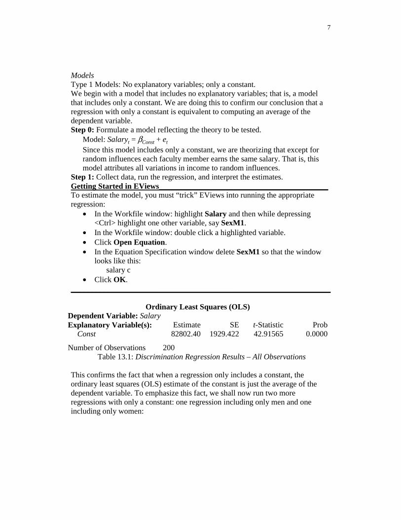
Models Type 1 Models: No explanatory variables; only a constant. We begin with a model that includes no explanatory variables; that is, a model that includes only a constant. We are doing this to confirm our conclusion that a regression with only a constant is equivalent to computing an average of the dependent variable. Step 0: Formulate a model reflecting the theory to be tested.
Model: Salaryt = βConst + et Since this model includes only a constant, we are theorizing that except for random influences each faculty member earns the same salary. That is, this model attributes all variations in income to random influences.
Step 1: Collect data, run the regression, and interpret the estimates. Getting Started in EViews___________________________________________ To estimate the model, you must “trick” EViews into running the appropriate regression:
• In the Workfile window: highlight Salary and then while depressing <Ctrl> highlight one other variable, say SexM1.
• In the Workfile window: double click a highlighted variable. • Click Open Equation. • In the Equation Specification window delete SexM1 so that the window
looks like this: salary c
• Click OK. __________________________________________________________________
Ordinary Least Squares (OLS) Dependent Variable: Salary Explanatory Variable(s): Estimate SE t-Statistic Prob Const 82802.40 1929.422 42.91565 0.0000 Number of Observations 200
Table 13.1: Discrimination Regression Results – All Observations
This confirms the fact that when a regression only includes a constant, the ordinary least squares (OLS) estimate of the constant is just the average of the dependent variable. To emphasize this fact, we shall now run two more regressions with only a constant: one regression including only men and one including only women:
Ordinary Least Squares (OLS) Dependent Variable: Salary Explanatory Variable(s): Estimate SE t-Statistic Prob Const 91840.58 2259.201 40.65180 0.0000 Number of Observations 137 Sample SexM1 = 1
Table 13.2: Discrimination Regression Results – Males Only
Ordinary Least Squares (OLS) Dependent Variable: Salary Explanatory Variable(s): Estimate SE t-Statistic Prob Const 63147.94 2118.879 29.80252 0.0000 Number of Observations 63 Sample SexM1 = 0
Table 13.3: Discrimination Regression Results – Females Only
Compare the regression results to the salary averages: Both males and females $82,802 Males only 91,841 Females only 63,148
Tables 13.1, 13.2, and 13.3 illustrate the important lesson that Type 1 models teach us. In a regression that includes only a constant, the ordinary least squares (OLS) estimate of the constant is the average of the dependent variable. Next, let us consider a slightly more complicated model.
9
Type 2 Models: A constant and a single dummy explanatory variable denoting sex. Step 0: Formulate a model reflecting the theory to be tested.
Salaryt = βConst + βSexM1SexM1t + et where SexM1 equals 1 for males and 0 for females
Discrimination Theory: Women are discriminated against in the job market; hence, men earn higher salaries than women. Since SexM1 equals 1 for males and 0 for females, βSexM1 should be positive indicating that men will earn more
than women: βSexM1 > 0. Step 1: Collect data, run the regression, and interpret the estimates.
Using the ordinary least squares (OLS) estimation procedure to estimate the parameters:
Ordinary Least Squares (OLS)
Dependent Variable: Salary Explanatory Variable(s): Estimate SE t-Statistic Prob SexM1 28692.65 3630.670 7.902852 0.0000 Const 63147.94 3004.914 21.01489 0.0000 Number of Observations 200 Estimated Equation: EstSalary = 63,148 + 28,693SexM1 Interpretation of Estimates: bSexM1= 28,693: Men earn $28,693 more than women. Critical Result: The SexM1 coefficient estimate equals 28,693. This evidence,
the positive sign of the coefficient estimate, suggests that men earn more than women thereby supporting the discrimination theory.
Table 13.4: Discrimination Regression Results – Male Sex Dummy
For emphasis, let us apply the estimated equation to men and then to women by plugging in their values for SexM1:
Estimated Equation: EstSalary = 63,148 + 28,693SexM1 We can now compute the estimated salary for men and women:
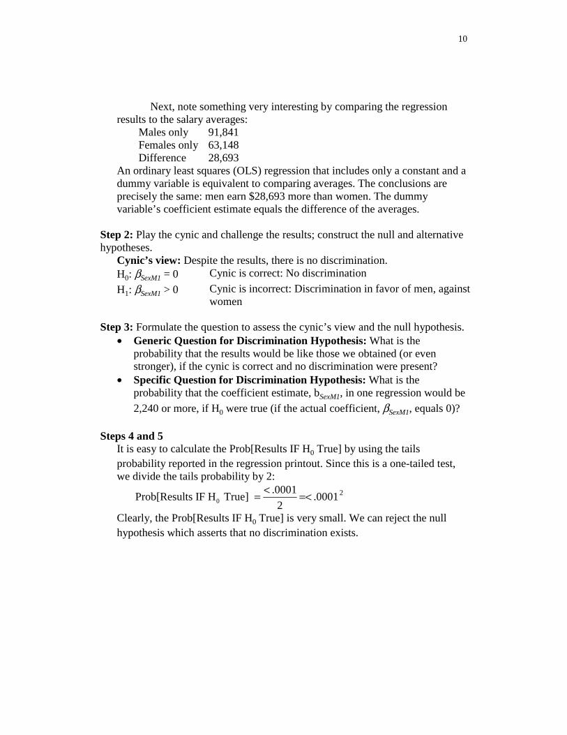
Next, note something very interesting by comparing the regression results to the salary averages:
Males only 91,841 Females only 63,148 Difference 28,693
An ordinary least squares (OLS) regression that includes only a constant and a dummy variable is equivalent to comparing averages. The conclusions are precisely the same: men earn $28,693 more than women. The dummy variable’s coefficient estimate equals the difference of the averages.
Step 2: Play the cynic and challenge the results; construct the null and alternative hypotheses.
Cynic’s view: Despite the results, there is no discrimination. H0: βSexM1 = 0 Cynic is correct: No discrimination
H1: βSexM1 > 0 Cynic is incorrect: Discrimination in favor of men, against women
Step 3: Formulate the question to assess the cynic’s view and the null hypothesis.
• Generic Question for Discrimination Hypothesis: What is the probability that the results would be like those we obtained (or even stronger), if the cynic is correct and no discrimination were present?
• Specific Question for Discrimination Hypothesis: What is the probability that the coefficient estimate, bSexM1, in one regression would be
2,240 or more, if H0 were true (if the actual coefficient, βSexM1, equals 0)? Steps 4 and 5
It is easy to calculate the Prob[Results IF H0 True] by using the tails probability reported in the regression printout. Since this is a one-tailed test, we divide the tails probability by 2:
0
.0001Prob[Results IF H True] .0001
2
<= =< 2
Clearly, the Prob[Results IF H0 True] is very small. We can reject the null hypothesis which asserts that no discrimination exists.
11
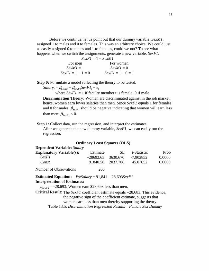
Before we continue, let us point out that our dummy variable, SexM1, assigned 1 to males and 0 to females. This was an arbitrary choice. We could just as easily assigned 0 to males and 1 to females, could we not? To see what happens when we switch the assignments, generate a new variable, SexF1:
Step 0: Formulate a model reflecting the theory to be tested.
Salaryt = βConst + βSexF1SexF1t + et where SexF1t = 1 if faculty member t is female; 0 if male
Discrimination Theory: Women are discriminated against in the job market; hence, women earn lower salaries than men. Since SexF1 equals 1 for females and 0 for males, βSexF1 should be negative indicating that women will earn less
than men: βSexF1 < 0. Step 1: Collect data, run the regression, and interpret the estimates.
After we generate the new dummy variable, SexF1, we can easily run the regression:
Ordinary Least Squares (OLS)
Dependent Variable: Salary Explanatory Variable(s): Estimate SE t-Statistic Prob SexF1 −28692.65 3630.670 -7.902852 0.0000 Const 91840.58 2037.708 45.07052 0.0000 Number of Observations 200 Estimated Equation: EstSalary = 91,841 − 28,693SexF1 Interpretation of Estimates: bSexF1= −28,693: Women earn $28,693 less than men. Critical Result: The SexF1 coefficient estimate equals −28,683. This evidence,
the negative sign of the coefficient estimate, suggests that women earn less than men thereby supporting the theory.
Table 13.5: Discrimination Regression Results – Female Sex Dummy
12
Let us apply this estimated equation to men and then to women by plugging in their values for SexF1:
For men For women SexF1 = 0 SexF1 = 1
EstSalaryMen = 91,841 − 0 = 91,841 EstSalaryWomen = 91,841 − 28,693 = 63,148 The results are precisely the same as before. This is reassuring. The decision to assign 1 to one group and 0 to the other group is completely arbitrary. It would be very discomforting if this arbitrary decision affected our conclusions. The fact that the arbitrary decision does not affect the results is crucial.
Step 2: Play the cynic and challenge the results; construct the null and alternative hypotheses.
Cynic’s view: Despite the results, there is no discrimination. H0: βSexF1 = 0 Cynic is correct: No discrimination
H1: βSexF1 < 0 Cynic is incorrect: Discrimination in favor of men, against women
The null hypothesis, like the cynic, challenges the evidence. The alternative hypothesis is consistent with the evidence.
Steps 3, 4, and 5
It is easy to calculate the Prob[Results IF H0 True] by using the tails probability reported in the regression printout. Since this is a one-tailed test, we divide the tails probability by 2:
0
.0001Prob[Results IF H True] .0001
2
<= =<
Since the probability is so small, we reject the null hypothesis that no discrimination exists.
Bottom Line
• Our choice of the base group for the dummy variable (that is, the group that is assigned a value of 0 for the dummy variable) does not influence the results.
• Type 2 models, models that include only a constant and a dummy variable, are equivalent to comparing averages.
13
Question: Do Type 2 models provide convincing evidence of gender discrimination?
• On the one hand, yes: o The dummy variable coefficients suggest that women earn less
than men. o The dummy variable coefficients are very significant – the
probability of obtaining results like we obtained if no discrimination exists is less than .0001.
• On the other hand, what implicit assumption is this discrimination model making? The model implicitly assumes that the only relevant factor in determining faculty salaries is gender. Is this reasonable? Well, very few individuals contend that gender is the only factor. Many individuals believe that gender is one factor, perhaps an important factor, affecting salaries, but they believe that other factors such as education, experience, etc. also play a role.
Type 3 Models: A constant, a dummy explanatory variable denoting sex, and other explanatory variable(s). While these models allow the possibility of gender discrimination, they also permit us to explore the possibility that other factors affect salaries too. To explore such models, let us include both a dummy variable and the number of years of experience as explanatory variables. Step 0: Formulate a model reflecting the theory to be tested.
Salaryt = βConst + βSexF1SexF1t + βExperExperiencet + et Theories:
• Discrimination: As before, we theorize that women are discriminated against: βSexF1 < 0.
• Experience: It is generally believed that in most occupations, employees with more experience earn more than employees with less experience. Consequently, we theorize that the experience coefficient should be positive: βExper > 0.
14
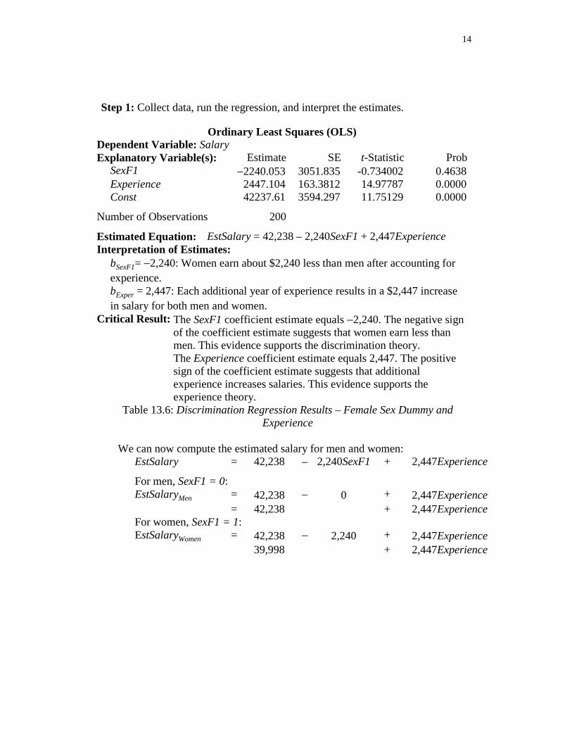
Step 1: Collect data, run the regression, and interpret the estimates.
Ordinary Least Squares (OLS) Dependent Variable: Salary Explanatory Variable(s): Estimate SE t-Statistic Prob SexF1 −2240.053 3051.835 -0.734002 0.4638 Experience 2447.104 163.3812 14.97787 0.0000 Const 42237.61 3594.297 11.75129 0.0000 Number of Observations 200 Estimated Equation: EstSalary = 42,238 – 2,240SexF1 + 2,447Experience Interpretation of Estimates: bSexF1= −2,240: Women earn about $2,240 less than men after accounting for
experience. bExper = 2,447: Each additional year of experience results in a $2,447 increase
in salary for both men and women. Critical Result: The SexF1 coefficient estimate equals −2,240. The negative sign
of the coefficient estimate suggests that women earn less than men. This evidence supports the discrimination theory.
The Experience coefficient estimate equals 2,447. The positive sign of the coefficient estimate suggests that additional experience increases salaries. This evidence supports the experience theory.
Table 13.6: Discrimination Regression Results – Female Sex Dummy and Experience
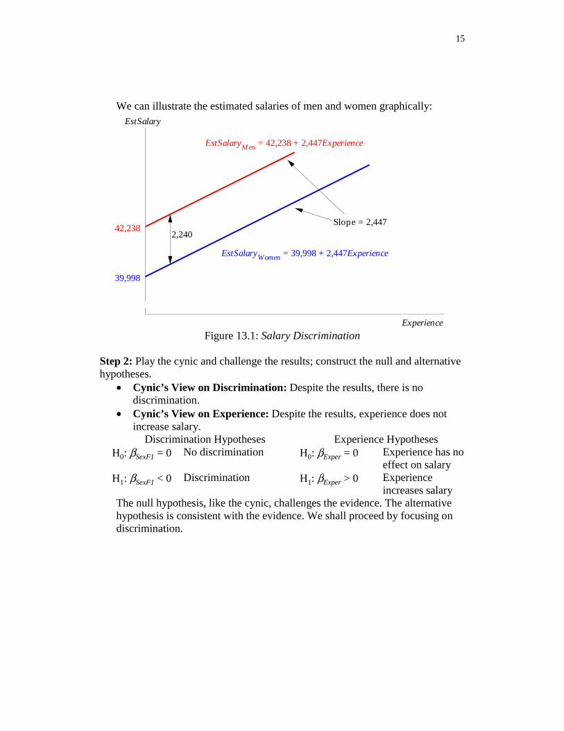
We can now compute the estimated salary for men and women:
increases salary The null hypothesis, like the cynic, challenges the evidence. The alternative hypothesis is consistent with the evidence. We shall proceed by focusing on discrimination.
16
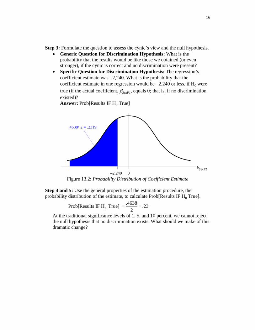
Step 3: Formulate the question to assess the cynic’s view and the null hypothesis. • Generic Question for Discrimination Hypothesis: What is the
probability that the results would be like those we obtained (or even stronger), if the cynic is correct and no discrimination were present?
• Specific Question for Discrimination Hypothesis: The regression’s coefficient estimate was −2,240. What is the probability that the coefficient estimate in one regression would be −2,240 or less, if H0 were
true (if the actual coefficient, βSexF1, equals 0; that is, if no discrimination existed)? Answer: Prob[Results IF H0 True]
0
.4638/2 = .2319
−2,240bSexF1
Figure 13.2: Probability Distribution of Coefficient Estimate
Step 4 and 5: Use the general properties of the estimation procedure, the probability distribution of the estimate, to calculate Prob[Results IF H0 True].
0
.4638Prob[Results IF H True] .23
2= =
At the traditional significance levels of 1, 5, and 10 percent, we cannot reject the null hypothesis that no discrimination exists. What should we make of this dramatic change?
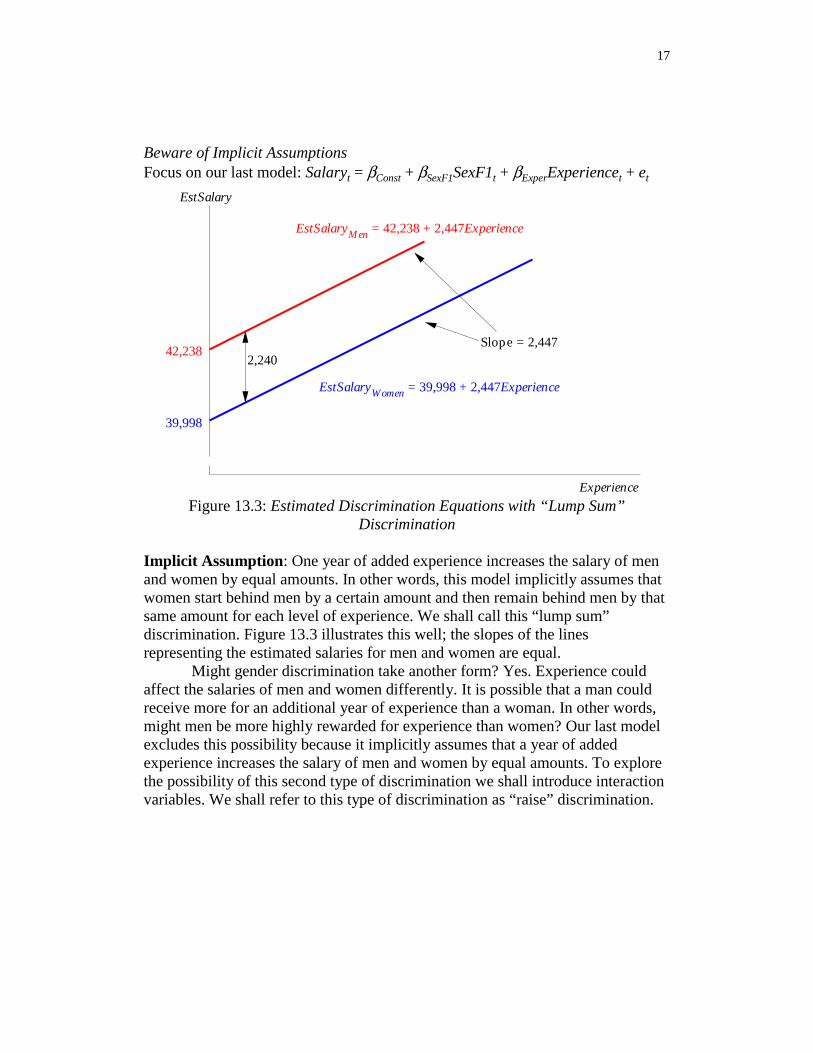
17
Beware of Implicit Assumptions Focus on our last model: Salaryt = βConst + βSexF1SexF1t + βExperExperiencet + et
39,998
42,238
EstSalaryMen = 42,238 + 2,447Experience
EstSalary
Experience
Slope = 2,447
EstSalaryWomen = 39,998 + 2,447Experience
2,240
Figure 13.3: Estimated Discrimination Equations with “Lump Sum”
Discrimination
Implicit Assumption: One year of added experience increases the salary of men and women by equal amounts. In other words, this model implicitly assumes that women start behind men by a certain amount and then remain behind men by that same amount for each level of experience. We shall call this “lump sum” discrimination. Figure 13.3 illustrates this well; the slopes of the lines representing the estimated salaries for men and women are equal.
Might gender discrimination take another form? Yes. Experience could affect the salaries of men and women differently. It is possible that a man could receive more for an additional year of experience than a woman. In other words, might men be more highly rewarded for experience than women? Our last model excludes this possibility because it implicitly assumes that a year of added experience increases the salary of men and women by equal amounts. To explore the possibility of this second type of discrimination we shall introduce interaction variables. We shall refer to this type of discrimination as “raise” discrimination.
18
Interaction Variables An interaction variable allows us to explore the possibility that one explanatory variable influences the effect that a second explanatory variable has on the dependent variable. We generate an interaction variable by multiplying the two variables together. We shall focus on the interaction of Experience and SexF1 by generating the variable Exper_SexF1:
Exper_SexF1 = Experience×SexF1 We shall now add the interaction variable, Exper_SexF1, to our last model. Step 0: Formulate a model reflecting the theory to be tested.
• “Lump Sum” Discrimination: As before, we theorize that women are discriminated against: βSexF1 < 0.
• Experience: As before, we theorize that the experience coefficient should be positive: βExper > 0.
• “Raise” Discrimination: One year of additional experience should increase the salary of women by less than their male counterparts. Hence, we theorize that the coefficient of the interaction variable is negative: βExper_SexF1 < 0. (If it is not clear why you should expect this coefficient to be negative, be patient. It should become clear shortly.)
Step 1: Collect data, run the regression, and interpret the estimates.
Figure 13.4: Estimated Discrimination Equations with “Lump Sum” and “Raise”
Discrimination
20
We can use this regression to assess the possibility of two different types of discrimination. One of the estimates is a little surprising:
• “Lump Sum” Discrimination: As before, the coefficient of the sex dummy variable, SexF1, assesses the possibility of “lump sum” discrimination. The coefficient estimate is positive. This is unexpected. It suggests that when faculty members are hired from graduate school with no experience, women receive about $10,970 more than men. The positive coefficient estimate suggests that reverse discrimination exists at the entry level.
• “Raise” Discrimination: The coefficient of the interaction variable, Exper_SexF1, assesses the possibility of this more subtle type of discrimination, “raise” discrimination. The coefficient estimate is negative. It suggests that a woman is receives $1,135 less than a man for an additional year of experience. The negative coefficient estimate suggests that women receive smaller annual raises than their male counterparts.
These regression results paint a more complex picture of possible discrimination than is often contemplated. Again, recall that as a consequence of privacy concerns these data were artificially generated. Consequently, do not conclude that the conclusions we have suggested here necessarily reflect the “real world.” This example was used because it illustrates how multiple regression analysis can exploit dummy variables and interaction variables to investigate important issues, such as the presence of discrimination. Conclusions
• Beware of Averages: We should not consider differences in averages, by themselves, as evidence of discrimination. When we just consider average salaries, we are implicitly adopting a model of salary determination that few, if anyone, consider realistic. We implicitly assume that the only factor that determines an individual’s salary is his/her sex. While many would argue that gender is one factor, very few would argue that gender is the only factor.
• Power of Multiple Regression Analysis: Since is it naïve to consider just averages what quantitative tools should we use to assess the presence of discrimination? Multiple regression analysis is an appropriate tool. It allows us to consider the roles played by several factors in the determination of salary and separates out the individual influence of each. Multiple regression analysis allows us to consider not only the role of gender, but also the role that the other factors may play. Multiple regression analysis sorts out the impact that each individual explanatory variable has on the dependent variable.
21
• Flexibility of Multiple Regression Analysis: Not only does multiple regression analysis allow us to consider the roles played by various factors in salary determination, but also it allows us to consider various types of potential discrimination. The above example illustrates how we can assess the possible presence “lump sum” discrimination and/or “raise” discrimination.
An Example: Internet and Television Use Next, we consider Internet and television use:
Project: Assess the determinants of Internet and television use internationally. Internet and TV Data: Panel data of Internet, TV, economic, and political statistics for 208 countries from 1995 to 2002.
[Link to MIT-InternetTVFlat-1995-2002.wf1 goes here.]
LogUsersInternett Logarithm of Internet users per 1,000 people for
observation t LogUsersTVt Logarithm of television users per 1,000 people for
observation t Yeart Year for observation t CapitalHumant Literacy rate for observation t (percent of literate
population 15 and over) CapitalPhysicalt Telephone mainlines per 10,000 people for observation t GdpPCt Per capita real GDP in nation t (1,000’s of “international”
dollars) Autht The Freedom House measures of political authoritarianism
for observation t normalized to a 0 to 10 scale. 0 represents the most democratic rating and 10 the most authoritarian. During the 1995-2002 period, Canada and the U.S. had a 0 rating; Iraq and the Democratic Republic of Korea (North Korea) rated 10.
Step 0: Formulate a model reflecting the theory to be tested. Internet Model: Int Int Int
t Const Year t CapHum t
Int Int Int IntCapPhy t GDP t Auth t t
LogUsersInternet Year CapitalHuman
CapitalPhysical GdpPC Auth e
β β β
β β β
= + + +
+ + +
Television Model: TV TV TVt Const Year t CapHum t
TV TV TV TVCapPhy t GDP t Auth t t
LogUsersTV Year CapitalHuman
CapitalPhysical GdpPC Auth e
β β β
β β β
= + + +
+ + +
The dependent variable in both the Internet and television models is the logarithm of users. This is done so that the coefficients can be interpreted as percentages.
Similarities and Differences The theory behind the effect of human capital, physical capital, and per capita GDP on both Internet and television use is straightforward: Additional human capital, physical capital, and per capita GDP should stimulate both Internet and television use.
We postulate that the impact of time and political factors should be
different for the two media, however: • As an emerging technology, we theorize that there should be substantial
growth of Internet use over time – even after accounting for all the other factors that may affect Internet use. Television, on the other hand, is a mature technology. After accounting for all the other factors, time should play little or no role in explaining television use.
• We postulate that the political factors should affect Internet and television use differently. Since authoritarian nations control the content of television, we would expect authoritarian nations to promote television; television provides the authoritarian nation the means to get the government’s message out. On the other hand, since it is difficult to control Internet content, we would expect authoritarian nations to suppress Internet use.
23
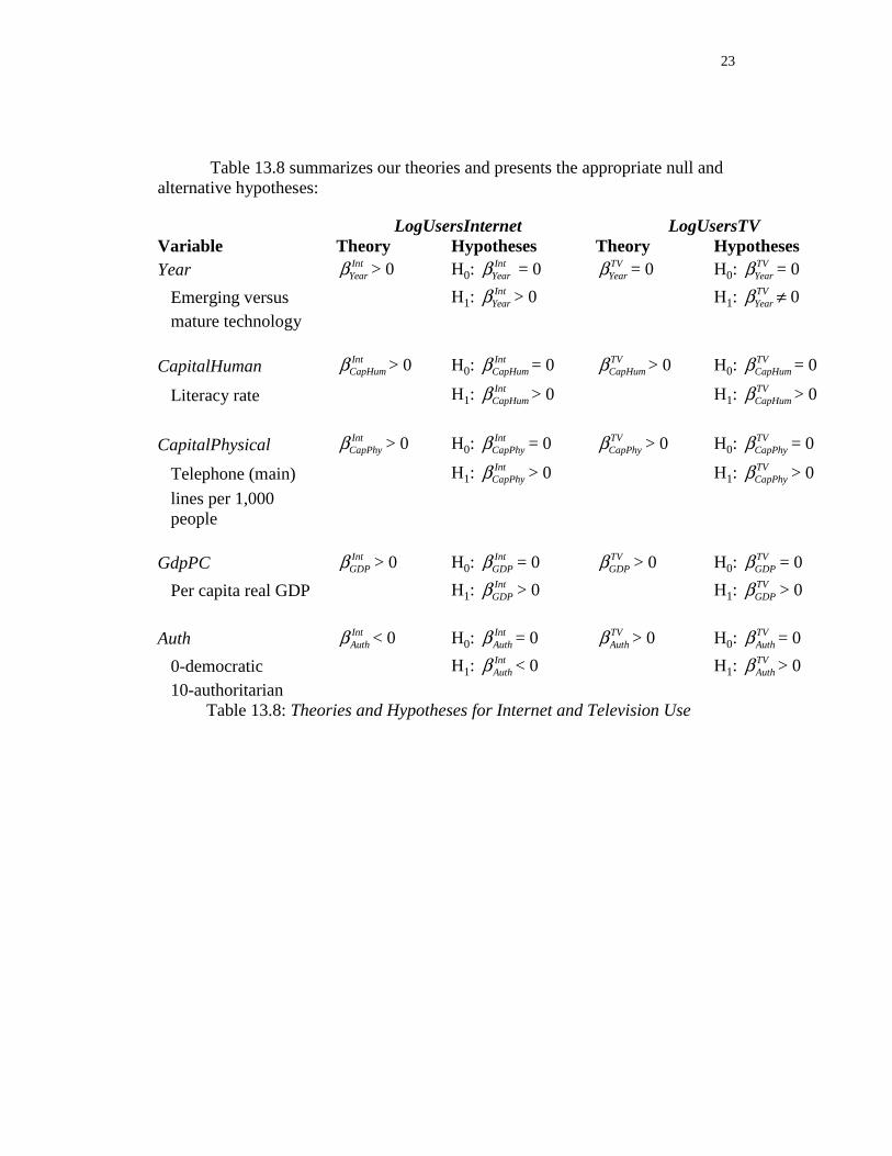
Table 13.8 summarizes our theories and presents the appropriate null and alternative hypotheses:
LogUsersInternet LogUsersTV Variable Theory Hypotheses Theory Hypotheses Year Int
Yearβ > 0 H0: Int
Yearβ = 0 TVYearβ = 0 H0:
TVYearβ = 0
Emerging versus H1: Int
Yearβ > 0 H1: TVYearβ ≠ 0
mature technology
CapitalHuman IntCapHumβ > 0 H0:
IntCapHumβ = 0 TV
CapHumβ > 0 H0: TVCapHumβ = 0
Literacy rate H1: IntCapHumβ > 0 H1:
TVCapHumβ > 0
CapitalPhysical IntCapPhyβ > 0 H0:
IntCapPhyβ = 0 TV
CapPhyβ > 0 H0: TVCapPhyβ = 0
Telephone (main) H1: Int
CapPhyβ > 0 H1: TVCapPhyβ > 0
lines per 1,000 people
GdpPC Int
GDPβ > 0 H0: IntGDPβ = 0 TV
GDPβ > 0 H0: TVGDPβ = 0
Per capita real GDP H1: IntGDPβ > 0 H1:
TVGDPβ > 0
Auth Int
Authβ < 0 H0: IntAuthβ = 0 TV
Authβ > 0 H0: TVAuthβ = 0
0-democratic H1: IntAuthβ < 0 H1:
TVAuthβ > 0
10-authoritarian Table 13.8: Theories and Hypotheses for Internet and Television Use
24
As Table 13.8 reports, all the hypothesis tests are one-tailed tests with the exception of the Year coefficient in the television use model.
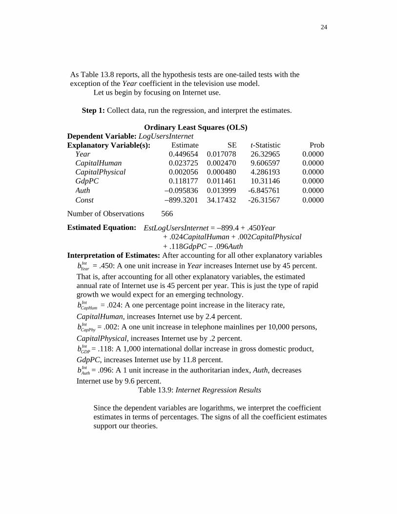
Let us begin by focusing on Internet use. Step 1: Collect data, run the regression, and interpret the estimates.
Interpretation of Estimates: After accounting for all other explanatory variables Int
Yearb = .450: A one unit increase in Year increases Internet use by 45 percent.
That is, after accounting for all other explanatory variables, the estimated annual rate of Internet use is 45 percent per year. This is just the type of rapid growth we would expect for an emerging technology.
IntCapHumb = .024: A one percentage point increase in the literacy rate,
CapitalHuman, increases Internet use by 2.4 percent. Int
CapPhyb = .002: A one unit increase in telephone mainlines per 10,000 persons,
CapitalPhysical, increases Internet use by .2 percent. Int
GDPb = .118: A 1,000 international dollar increase in gross domestic product,
GdpPC, increases Internet use by 11.8 percent. Int
Authb = .096: A 1 unit increase in the authoritarian index, Auth, decreases
Internet use by 9.6 percent. Table 13.9: Internet Regression Results
Since the dependent variables are logarithms, we interpret the coefficient estimates in terms of percentages. The signs of all the coefficient estimates support our theories.
Interpretation of Estimates: After accounting for all other explanatory variables TV
Yearb = .023: A one unit increase in Year increases television use by 2.3
percent. The tails probability indicates that after accounting for all other explanatory variables, we cannot reject the null hypothesis that there is no growth in television use at the traditional significance levels. This is what we would expect for a mature technology.
TVCapHumb = .036: A one percentage point increase in the literacy rate,
CapitalHuman, increases television use by 3.6 percent. TV
CapPhyb = .002: A one unit increase in telephone mainlines per 10,000 persons,
CapitalPhysical, increases television use by .2 percent. TV
GDPb = .058: A 1,000 international dollar increase in gross domestic product,
GdpPC, increases television use by 5.9 percent. TV
Authb = .063: A 1 unit increase in the authoritarian index, Auth, increases
television use by 6.3 percent. Table 13.10: Television Regression Results
26
Steps 2, 3, 4, and 5: Table 13.11 summarizes the remaining steps:
LogUsersInternet LogUsersTV Year .450* .023 (<.0001) (.1487) CapitalHuman .024* .036* (<.0001) (<.0001) CapitalPhysical .002* .002* (<.0001) (.0001) GdpPC .118* .059* (<.0001) (<.0001) Auth −.096* .064* (<.0001) (<.0001) Prob[Results IF H0 True] in parentheses. * indicates significance at the 1 percent level.
Table 13.11: Coefficient Estimates and Prob[Results IF H0 True]
Note that all the results support the theories and all the coefficients except for the Year coefficient in the television regression are significant at the 1 percent level. It is noteworthy that the regression results suggest that the impact of Year and Auth differ for the two media just as we postulated. Our results suggest that after accounting for all other explanatory variables:
• Internet use grows by an estimated 45 percent whereas the growth rate of television use does not differ significantly from 0.
• Increases in the authoritarian index results to a significant decrease Internet use, but a significant increase television use.
27
Interaction Variable: Economic and Political Interaction Next, let us investigate the following question:
Question: Does per capita GDP have a greater impact on Internet use in authoritarian nations than non-authoritarian ones?
Some argue that the answer to this question is yes; that is, that per capita GDP has a greater impact on Internet use in authoritarian nations. Their rationale is based on the following logic:
In authoritarian nations, citizens have few sources of uncensored information. There are few, if any, uncensored newspapers, news magazines, etc. available. The only source of uncensored information is the Internet. Consequently, the effect of per capita GDP on Internet use will be large.
In non-authoritarian nations, citizens have many sources of uncensored information. Higher per capita GDP will no doubt stimulate Internet use, but it will also stimulate the purchase of uncensored newspapers, news magazines, etc. Consequently, the effect on Internet use will be modest.
An authoritarian index-GDP interaction variable can be used to explore this issue. To do so, generate the interaction variable Auth_GdpPC, the product of the authoritarian index and per capita GDP:
Auth_GdpPC = Auth×GdpPC Step 0: Formulate a model reflecting the theory to be tested.
Add this interaction variable to the Internet model:
_ _
Int Int Intt Const Year t CapHum t
Int Int Int Int IntCapPhy t GDP t Auth t Auth GDP t t
LogUsersInternet Year CapitalHuman
CapitalPhysical GdpPC Auth Auth GdpPC e
β β β
β β β β
= + + +
+ + + +
If the theory regarding the interaction of authoritarianism and per capita GDP is correct, the coefficient of the interaction variable, Auth_GdpPC, should positive: _ 0Int
Auth GDPβ > . (If you are not certain why, it should
become clear shortly.) The null and alternative hypotheses are: H0: _ 0Int
Auth GDPβ =
H1: _ 0IntAuth GDPβ >
28
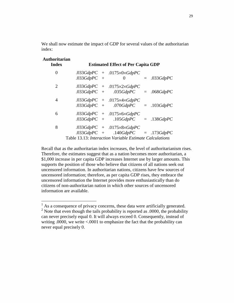
Step 1: Collect data, run the regression, and interpret the estimates.
Recall that as the authoritarian index increases, the level of authoritarianism rises. Therefore, the estimates suggest that as a nation becomes more authoritarian, a $1,000 increase in per capita GDP increases Internet use by larger amounts. This supports the position of those who believe that citizens of all nations seek out uncensored information. In authoritarian nations, citizens have few sources of uncensored information; therefore, as per capita GDP rises, they embrace the uncensored information the Internet provides more enthusiastically than do citizens of non-authoritarian nation in which other sources of uncensored information are available.
1 As a consequence of privacy concerns, these data were artificially generated. 2 Note that even though the tails probability is reported as .0000, the probability can never precisely equal 0. It will always exceed 0. Consequently, instead of writing .0000, we write <.0001 to emphasize the fact that the probability can never equal precisely 0.