Chapter 16 Natural resources and economic growth - kuweb.econ.ku.dk/okocg/VV/VV-2014/Lectures and...

Chapter 16

Natural resources and

economic growth

In this course, up to now, the relationship between economic growth and the

earth’s finite natural resources has been touched upon in connection with: the

discussion of returns to scale (Chapter 2), the transition from a pre-industrial

to an industrial economy (in Chapter 7), and the environmental problem of

global warming (Chapter 8). In a more systematic way the present chapter

reviews how natural resources, including the environment, relate to economic

growth.

The contents are:

• Classification of means of production.

• The notion of sustainable development.

• Renewable natural resources.

• Non-renewable natural resources.

• Natural resources and the issue of limits to economic growth.

The first two sections aim at establishing a common terminology for the

discussion.

16.1 Classification of means of production

We distinguish between different categories of production factors, also called

means of production. First the two broad categories:

273

274

CHAPTER 16. NATURAL RESOURCES AND ECONOMIC

GROWTH

1. Producible means of production, also called man-made inputs.

2. Non-producible means of production.

The first category includes:

1.1 Physical inputs like processed raw materials, intermediate goods, ma-

chines, and buildings.

1.2 Human inputs of a produced character like technical knowledge (avail-

able in books, USB sticks etc.) and human capital.

The second category includes:

2.1 Human inputs of a non-produced character, sometimes called “raw la-

bor”.1

2.2 Natural resources. By definition in limited supply on this earth.

Natural resources can be sub-divided into:

2.2.1 Renewable resources, that is, natural resources the stock of which can

be replenished by a natural self-regeneration process. Hence, if the

resource is not over-exploited, it can be sustained in a more or less

constant amount. Examples: ground water, fertile soil, fish in the sea,

clean air, national parks.

2.2.2 Non-renewable resources, that is, natural resources which have no nat-

ural regeneration process (at least not within a relevant time scale).

The stock of a non-renewable resource is thus depletable. Examples:

fossil fuels, many non-energy minerals, virgin wilderness, endangered

species, ozone layer.

The climate change problem due to greenhouse gasses can be seen as be-

longing to somewhere between category 2.2.1 or 2.2.2 in that the atmosphere

has a natural self-regeneration ability, but the speed of regeneration is very

low.

Given the scarcity of natural resources and the pollution problems caused

by economic activity, key issues are:

a. Is sustainable development possible?

b. Is sustainable economic growth (in a per capita welfare sense) possible?

But what does “sustainable” and “sustainability” really mean”?

1Outside a slave society, biological reproduction is usually not considered as part of the

economic sphere of society even though formation and maintainance of raw labor requires

child rearing, health, food etc. and is thus conditioned by economic circumstances.

c° Groth, Lecture notes in Economic Growth, (mimeo) 2014.

16.2. The notion of sustainable development 275

16.2 The notion of sustainable development

The basic idea in the notion of sustainable development is to emphasize

intergenerational responsibility. The Brundtland Commission (1987) defined

sustainable development as “development that meets the needs of present

generations without compromising the ability of future generations to meet

theirs”.

In more standard economic terms we may define sustainable economic

development as a time path along which per capita welfare remains non-

decreasing across generations forever. An aspect of this is that current eco-

nomic activities should not impose significant economic risks on future gen-

erations. The “forever” in the definition can not, of course, be taken literally,

but as equivalent to “for a very long time horizon”. We know that the sun

will eventually (in some billion years) burn out and consequently life on earth

will become extinct.

Note also that our definition emphasizes welfare, which should be under-

stood in a broad sense, that is, as more or less synonymous with “quality of

life”, “living conditions”, or “well-being” (the term used in Smulders, 1995).

What may matter is thus not only the per capita amount of marketable con-

sumption goods, but also things like health, life expectancy, enjoyment of

services from the ecological system, and capability to lead a worthwhile live.

To make this more specific, consider the period utility function of a typical

individual. Suppose two variables enter as arguments, namely consumption,

of a marketable produced good and some measure, of the quality of

services from the eco-system. Suppose further that the period utility function

is of CES form:2

( ) =£ + (1− )

¤1 0 1 1 (16.1)

The parameter is called the substitution parameter. The elasticity of substi-

tution between the two goods is = 1(1−) 0 a constant. When → 1

(from below), the two goods become perfect substitutes (in that → ∞).The smaller is the less substitutable are the two goods. When 0 we

have 1 and as → −∞ the indifference curves become near to right

angled.3 According to many environmental economists, there are good rea-

2CES stands for Constant Elasticity of Substitution.3By L’Hôpital’s rule for “0/0” it follows that, for fixed and

lim→0 6=0

£ + (1− )

¤1= 1−

So the Cobb-Douglas utility function, which has elasticity of substitution between the

goods equal to 1, is an intermediate case, corresponding to = 0. More details in the


276


GROWTH

sons to believe that 1, since water, basic foodstuff, clean air, absence of

catastrophic climate change, etc. are difficult to replace by produced goods

and services. In this case there is a limit to the extent at which a rising ,

along with a rising per capita income, can compensate for falling

At the same time the techniques by which the ordinary consumption

good is currently produced may be “dirty” and thereby cause a falling . An

obvious policy response is the introduction of pollution taxes that increase the

incentive for firms to replace these techniques with cleaner ones. For certain

forms of pollution (e.g., sulfur dioxide, SO2 in the air) there is evidence of an

inverted U-curve relationship between the degree of pollution and the level

of economic development measured by GDP per capita − the environmentalKuznets curve.

So an important element in sustainable economic development is that the

economic activity of current generations does not spoil the environmental

conditions for future generations. Living up to this requirement necessitates

economic and environmental strategies consistent with the planet’s endow-

ments. This means recognizing the role of environmental constraints for eco-

nomic development. A complicating factor is that specific abatement policies

vis-a-vis particular environmental problems may face resistance from interest

groups.

As defined, a criterion for sustainable economic development to be present

is that per capita welfare remains non-decreasing across generations. A sub-

category of this is sustainable economic growth which is present if per capita

welfare is growing across generations. Here we speak of growth in a welfare

sense, not in a physical sense. Permanent exponential per capita output

growth in a physical sense is of course not possible with limited natural re-

sources (matter or energy). The issue about sustainable growth is whether,

by combining the natural resources with man-made inputs (knowledge, hu-

man capital, and physical capital), an output stream of increasing quality,

and therefore increasing economic value, can be maintained. In modern times

capabilities of many digital electronic devices provide conspicuous examples

of exponential growth in quality (or efficiency). Think of processing speed,

memory capacity, and efficiency of electronic sensors. What is known as

Moore’s Law is the rule of thumb that there is a doubling of the efficiency of

microprocessors within every 18 months. The evolution of the internet has

provided faster and widened dissemination of information and fine arts.

Of course there are intrinsic difficulties associated with measuring sus-

tainability in terms of well-being. There now exists a large theoretical and

applied literature dealing with these issues. A variety of extensions and

appendix.


16.3. Renewable resources 277

modifications of the standard national income accounting GDP has been de-

veloped under the heading Green NNP (green net national product). An

essential feature in the measurement of Green NNP is that from the conven-

tional GDP (which essentially just measures the level of economic activity) is

subtracted the depreciation of not only the physical capital but also the en-

vironmental assets. The latter depreciate due to pollution, overburdening of

renewable natural resources, and depletion of reserves of non-renewable nat-

ural resources.4 In some approaches the focus is on whether a comprehensive

measure of wealth is maintained over time. Along with reproducible assets

and natural assets (including the damage to the atmosphere from greenhouse

gasses), Arrow et al. (2012) take in health, human capital, and “knowledge

capital” in their measure of “wealth”. They apply this measure in a study

of the United States, China, Brazil, India, and Venezuela over the period

1995-2000 and find that all five countries satisfy the sustainability criterion

of non-decreasing wealth in this broad sense. Indeed their wealth measure is

found to be growing in all five countries.5 Note that it is sustainability that

is claimed, not optimality.

In the next two sections we will go more into detail with the challenge

to sustainability and growth coming from renewable and non-renewable re-

sources, respectively. We shall primarily deal with the issues from the point of

view of technical feasibility of non-decreasing, and possibly rising, per-capita

consumption. Concerning the big questions about appropriate institutions

the reader is referred to the specialized literature.

We begin with renewable resources.

16.3 Renewable resources

A useful analytical tool is the following simple model of the stock dynamics

associated with a renewable resource.

Let ≥ 0 denote the stock of the renewable resource at time Then wemay write

≡

= − = ()− (16.2)

4The depreciation of these environmental and natural assets is evaluated in terms of

the social planner’s shadow prices. See, e.g., Heal (1998), Weitzman (2001, 2003), and

Stiglitz et al. (2010).5Of course, many measurement uncertainties and disputable issues of weighting are

involved; brief discussions, and questioning, of the study are contained in Solow (2012),

Hamilton (2012), and Smulders (2012). Regarding Denmark 1990-2009, a study by Lind

and Schou (2013), along lines somewhat similar to those of Arrow et al. (2012), also

suggests sustainability to hold.


278


GROWTH

where is the self-regeneration of the resource per time unit and ≥ 0 isthe extraction (and use) of the resource per time unit at time . If for instance

the stock refers to the number of fish in the sea, the flow represents the

number of fish caught per time unit. And if, in a pollution context, the stock

refers to “cleanness” of the air in cities, measures, say, the emission of

sulfur dioxide, SO2, per time unit. The self-regenerated amount per time

unit depends on the available stock through the function () known as a

self-regeneration function.6

Until further notice, we stick to the first interpretation, that of indi-

cating the size of a fish population. The self-regeneration function will often

have a bell-shape as illustrated in the upper panel of Figure 16.1. Essentially,

the self-regeneration ability is due to the flow of solar energy continuously

entering the the eco-system of the earth. This flow of solar energy is constant

and beyond human control.

There is a lower threshold, (0) ≥ 0 below which even with = 0 thereare too few female fish to generate offspring, and the population necessar-

ily shrinks and eventually reaches zero. We may call (0) the minimum

sustainable stock.

At the other intersection with the horizontal axis, (0) represents the

maximum sustainable stock. The eco-system cannot support further growth

in the fish population. The reason may be food scarcity or spreading of

diseases because of high population density.7 The value indicated on

the vertical axis, in the upper panel equals = max (). This value is thus

the maximum sustainable yield per time unit. It is sustainable, presupposing

the size of the fish population is initially at least of size = argmax ()

which is that value of where () = The size, of the fish

population is consistent with maintaining the harvest per time unit

forever in a steady state.

The lower panel in Figure 16.1 illustrates the dynamics in the ( ) plane,

given a fixed level of = ∈ (0 ]. The arrows indicate the direction

of movement. In the long run, if = for all the stock will settle down

at the size () The stippled curve in the upper panel indicates ()−

which is the same as in the lower panel which presumes = . The

stippled curve in the lower panel indicates the dynamics in case = .

In this case the steady-state stock, ( ) = , is unstable. In this

6Even if represents the stock of a non-renewable resource, the equation (16.2) will

still be valid if we impose that there is no self-regeneration, i.e., () ≡ 0.7Popular mathematical specifications of (·) include the logistic function () =

(1−) where 0 0 and the quasi-logistic function() = (1−)(−1) where also 0 In both cases (0) = but (0) equals 0 in the first case and in

the second.



G

( )G S

O (0)S MSYS (0)S S

MSY

S

MSYS

( )G S R

( )G S R

O

R

S ( )S R

( )G S MSY

Figure 16.1: The self-generation function (upper panel) and stock dynamics for

= ∈ (0 ] (lower panel).


280


GROWTH

state a small negative shock to the stock will not lead to a gradual return

but to a self-reinforcing reduction of the stock as long as the extraction

= is maintained.

is an ecological maximum and not necessarily in any sense an eco-

nomic optimum. Indeed, since the search and extraction costs may be a

decreasing function of the fish density, hence of the stock, it may be worth-

while to increase the stock beyond , thus settling for a smaller harvest

per time unit. Moreover, a microeconomic calculation will maximize the

sum of discounted expected profits per time unit, taking into account the

expected evolution of the market price of fish, the cost function, and the

dynamic relationship (16.2).

In addition to its importance for regeneration, the stock, may have

amenity value and thus enter the instantaneous utility function. Then again

some conservation of the stock over and above will be motivated.

A dynamic model with a renewable resource Consider a simple model

consisting of (16.2) together with

= ( ) ≥ 0 = − − ≥ 0 0 0 given,

= 0 ≥ 0 (16.3)

where is aggregate output and , and are inputs of capital, labor,

and a renewable resource, respectively, per time unit at time Let the aggre-

gate production function, be neoclassical8 with constant returns to scale

w.r.t. the rival inputs and The assumption ≥ 0 representsexogenous technical progress. Further, is aggregate consumption (≡

where is per capita consumption) and denotes a constant rate of capital

depreciation. There is no distinction between employment and population,

. The population growth rate, is assumed constant.

Is sustainable economic development in this setting technically feasible?

The answer will be yes if non-decreasing per capita consumption can be

sustained forever. As the issue is about technical feasibility, we disregard

problems of “tragedy of the commons”. Or rather, we assume this problem

is avoided by appropriate institutions.

Suppose the use of the renewable resource is kept constant at a sustainable

level ∈ (0 ). To begin with, suppose = 0 so that = for all

≥ 0 Assume that at = the system is “productive” in the sense that

lim→0

( 0) lim→∞

( 0) (A1)

8That is, marginal productivities of the production factors are positive, but diminishing;

and the upper contour sets are strictly convex.



Y

( , , , 0)F K L R

O

C

K K K

K

Figure 16.2: Sustainable consumption in the case of = 0 and no technical progress

( and fixed).

This condition is satisfied in Figure 16.2 where the value has the property

( 0) = Given the circumstances, this value is the least upper

bound for a sustainable capital stock in the sense that

if ≥ we have 0 for any 0 while

if 0 we have = 0 for = ( 0)− 0

For such a illustrated in Figure 16.2, a constant = ( 0) is main-

tained forever which implies non-decreasing per-capita income, ≡ ,

forever. So, in spite of the limited availability of the natural resource, a non-

decreasing level of consumption is technically feasible even without technical

progress. A forever growing level of consumption will, of course, require

sufficient technical progress capable of substituting for the natural resource.

Now consider the case 0 Along a balanced growth path (if it exists)

we have

1 = (

) (16.4)

where and must be constant, cf. Chapter 4. Maintaining

(= ()()) constant along this path when 0 requires that is constant and thereby that grows at the rate But then will be

declining over time. To compensate for this in (16.4), sufficient technical


282


GROWTH

progress is necessary. This of course holds, a fortiori, for sustained growth in

per-capita consumption to occur.

As technical progress in the far future is by its very nature uncertain and

unpredictable, there can be no guarantee for sustained per capita growth.

Pollution As hinted at above, the concern that certain production meth-

ods involve pollution is commonly incorporated into economic analysis by

subsuming environmental quality into the general notion of renewable re-

sources. In that context in (16.2) and Figure 16.1 will represent the “level

of environmental quality” and will be the amount of dirty emissions per

time unit. Since the level of the environmental quality is likely to be an

argument in both the utility function and the production function, again

some limitation of the “extraction” (the pollution flow) is motivated. Pol-

lution taxes may help to encourage abatement activities and make technical

innovations towards cleaner production methods more profitable.

16.4 Non-renewable resources

Whereas extraction and use of renewable resources can be sustained at a

more or less constant level (if not too high), the situation is different with

non-renewable resources. They have no natural regeneration process (at least

not within a relevant time scale) and so continued extraction per time unit

of these resources will inevitably have to decline and approach zero in the

long run.

To get an idea of the implications, we will consider the Dasgupta-Heal-

Solow-Stiglitz model (DHSS model) from the 1970s.9

16.4.1 The DHSS model

The production side of the model is described by:

= ( ) ≥ 0 (16.5)

= − − ≥ 0 0 0 given, (16.6)

= − ≡ − 0 0 given, (16.7)

= 0 ≥ 0 (16.8)

The new element is the replacement of (16.2) with (16.7), where is the

stock of the non-renewable resource (e.g., oil reserves), and is the depletion

9See, e.g., Stiglitz, 1974.


16.4. Non-renewable resources 283

rate. Since we must have ≥ 0 for all there is a finite upper bound oncumulative resource extraction:Z ∞

0

≤ 0 (16.9)

Since the resource is non-renewable, no re-generation function appears in

(16.7). Uncertainty is ignored and the extraction activity involve no costs.10

As before, there is no distinction between employment and population, .

The model was formulated as a response to the pessimistic Malthusian

views of the Club of Rome (Meadows et al., 1972). Stiglitz (and fellow econo-

mists) asked the question: what are the technological conditions needed to

avoid falling per capita consumption in the long run in spite of the inevitable

decline in resource use? The answer is that there are three ways in which

this decline in resource use may be counterbalanced:

1. input substitution;

2. resource-saving technical progress;

3. increasing returns to scale.

Let us consider each of them in turn (although in practice the three

mechanisms tend to be intertwined).

Input substitution

By input substitution is meant the gradual replacement of the input of the

exhaustible natural resource by man-made input, capital. Substitution of fos-

sil fuel energy by solar, wind, tidal and wave energy resources is an example.

Similarly, more abundant lower-grade non-renewable resources can substitute

for scarce higher-grade non-renewable resources - and this will happen when

the scarcity price of these has become sufficiently high. A rise in the price

of a mineral makes a synthetic substitute cost-efficient or lead to increased

recycling of the mineral. Finally, the composition of final output can change

toward goods with less material content. Overall, capital accumulation can

be seen as the key background factor for such substitution processes (though

also the arrival of new technical knowledge may be involved - we come back

to this).

10This simplified description of resource extraction is the reason that it is common

to classify the model as a one-sector model, notwithstanding there are two productive

activities in the economy, manufacturing and resource extraction.


284


GROWTH

Whether capital accumulation can do the job depends crucially on the

degree of substitutability between and To see this, let the produc-

tion function be a three-factor CES production function. Suppressing the

explicit dating of the variables when not needed for clarity, we have.

=¡1

+ 2 + 3

¢1

1 2 3 0 1+2+3 = 1 1 6= 0(16.10)

The important parameter is the substitution parameter. Let denote the

cost to the firm per unit of the resource flow and let be the cost per unit

of capital (generally, = + where is the real rate of interest). Then

is the relative factor price, which may be expected to increase as the

resource becomes more scarce. The elasticity of substitution between and

is [()()] ( )() evaluated along an isoquant curve,

i.e., the percentage rise in the - ratio that a cost-minimizing firm will

choose in response to a one-percent rise in the relative factor price,

Since we consider a CES production function, this elasticity is a constant

= 1(1 − ) 0 Indeed, the three-factor CES production function has

the property that the elasticity of substitution between any pair of the three

production factors is the same.

First, suppose 1 i.e., 0 1 Then, for fixed and →¡1

+ 2¢1

0 when → 0 In this case of high substitutability the

resource is seen to be inessential in the sense that it is not necessary for a

positive output. That is, from a production perspective, conservation of the

resource is not vital.

Suppose instead 1 i.e., 0 Although increasing when decreases,

output per unit of the resource flow is then bounded from above. Conse-

quently, the finiteness of the resource inevitably implies doomsday sooner or

later if input substitution is the only salvage mechanism. To see this, keeping

and fixed, we get

= (−)1 =

∙1(

) + 2(

) + 3

¸1→ 3

1 for → 0

(16.11)

since 0 Even if and are increasing, lim→0 = lim→0()=

13 · 0 = 0 Thus, when substitutability is low, the resource is essential

in the sense that output is nil in the absence of the resource.

What about the intermediate case = 1? Although (16.10) is not de-

fined for = 0 using L’Hôpital’s rule (as for the two-factor function, cf.

Appendix), it can be shown that¡1

+ 2 + 3

¢1 → 123

for → 0 In the limit a three-factor Cobb-Douglas function thus appears.

This function has = 1 corresponding to = 0 in the formula = 1(1−)



The interesting aspect of the Cobb-Douglas case is that it is the only

case where the resource is essential while at the same time output per unit

of the resource is unbounded from above (since = 123−1 → ∞for → 0).11 Under these circumstances it was considered an open question

whether non-decreasing per capita consumption could be sustained. There-

fore the Cobb-Douglas case was studied intensively. For example, Solow

(1974) showed that if = = 0, then a necessary and sufficient condition

that a constant positive level of consumption can be sustained is that 1 3

This condition in itself seems fairly realistic, since, empirically, 1 is many

times the size of 3 (Nordhaus and Tobin, 1972, Neumayer 2000). Solow

added the observation that under competitive conditions, the highest sus-

tainable level of consumption is obtained when investment in capital exactly

equals the resource rent, · This result was generalized in Hartwick(1977) and became known as Hartwick’s rule. If there is population growth

( 0) however, not even the Cobb-Douglas case allows sustainable per

capita consumption unless there is sufficient technical progress, as equation

(16.15) below will tell us.

Neumayer (2000) reports that the empirical evidence on the elasticity of

substitution between capital and energy is inconclusive. Ecological econo-

mists tend to claim the poor substitution case to be much more realistic

than the optimistic Cobb-Douglas case, not to speak of the case 1 This

invites considering the role of technical progress.

Technical progress

Solow (1974) and Stiglitz (1974) analyzed the theoretical possibility that

resource-saving technological change can overcome the declining use of non-

renewable resources that must be expected in the future. In this context

the focus is not only on whether a non-decreasing consumption level can

be maintained, but also on the possibility of sustained per capita growth in

consumption.

New production techniques may raise the efficiency of resource use. For

example, Dasgupta (1993) reports that during the period 1900 to the 1960s,

the quantity of coal required to generate a kilowatt-hour of electricity fell

from nearly seven pounds to less than one pound.12 Further, technological

developments make extraction of lower quality ores cost-effective and make

more durable forms of energy economical. On this background we incorpo-

rate resource-saving technical progress at the rate 3 along with labor-saving

11To avoid misunderstanding: by “Cobb-Douglas case” we refer to any function where

enters in a “Cobb-Douglas fashion”, i.e., any function like = ()1−33 12For a historical account of energy technology, see Smil (1994).


286


GROWTH

technical progress at the rate 2 So the CES production function reads

=¡1

+ 2(2) + 3(3)

¢1

(16.12)

where 2 = 2 and 3 = 3 assuming 2 and 3 to be exogenous positive

constants. If the (proportionate) rate of decline of is kept smaller than

3 then the “effective” resource input is no longer decreasing over time. As

a consequence, even if 1 (the poor substitution case), the finiteness of

nature need not be an insurmountable obstacle to non-decreasing per capita

consumption.

Actually, a technology with 1 needs a considerable amount of resource-

saving technical progress to obtain compliance with the empirical fact that

the income share of natural resources has not been rising (Jones, 2002). When

1 market forces tend to increase the income share of the factor that is

becoming relatively more scarce. Empirically, and have increased

systematically. However, with a sufficiently increasing 3, the income share

need not increase in spite of 1 Similarly, for the model to comply

with Kaldor’s “stylized facts” (more or less constant growth rates of and

and stationarity of the output-capital ratio, the income share of labor,

and the rate of return on capital), we need labor-saving technical change (2growing over time).13 The motivation for not introducing a rising 1 and

replacing in (16.12) by 1 is that this would be at odds with Kaldor’s

“stylized facts”, in particular the absence of a trend in the rate of return to

capital.

With 3 2 + we end up with conditions allowing a balanced growth

path (BGP for short), defined as a path along which the quantities

and change at constant proportionate rates (some or all of which may be

negative). It is well-known that compliance with Kaldor’s “stylized facts”

is close to equivalent to existence of a balanced growth path. It can be

shown that along the BGP, (2) is constant and so = 2 (hence also

= 2)14 Of course, one thing is that such a combination of assumptions

allows for constant growth in per capita consumption - which is more or less

what we have seen since the industrial revolution. Another thing is: will the

needed assumptions be satisfied for a long time in the future? Since we have

considered exogenous technical change, there is so far no hint from theory.

But, even taking endogenous technical change into account, there will be

many uncertainties about what technological changes will come through in

the future and how fast.

13Although the two forms of technical change are by many authors called “resource-

augmenting” and “labor-augmenting”, respectively, we prefer the more intuitive names,

“resource-saving” and “labor-saving”.14For any positive variable , denotes the growth rate, .



Balanced growth in the Cobb-Douglas case Let us end this discussion

by some remarks about the Cobb-Douglas case. By making capital-saving,

labor-saving, and resource-saving technical progress indistinguishable, the

Cobb-Douglas case again constitutes a convenient intermediate case. Tech-

nical progress can simply be represented by

= 123 1 2 3 0 1 + 2 + 3 = 1 (16.13)

where total factor productivity, , is growing over time. This, together with

(16.6) - (16.8), is now the model under examination.

Let us assume grows at some constant rate 0 Log-differentiating

w.r.t. time in (16.13) yields the growth-accounting relation

= + 1 + 2+ 3 (16.14)

By a simple extension of the method in Chapter 4, it is easily shown that

along a BGP, = = ≡ + and, if nothing of the resource is left

unutilized forever, = ≡ = − = constant 015 With the

depletion rate, denoted (16.14) thus implies

= =1

1− 1( − 3− 3) (16.15)

since 1 + 2 − 1 = −3Absent the need for input of limited natural resources, we would have

3 = 0 and so = (1−1) But with 3 0 the non-renewable resource

is essential and implies a drag on per capita growth equal to 3(+)(1−1).We get 0 if and only if 3(+ ) (where, the depletion rate, can

in principle be chosen very small if we want a strict conservation policy).

It is noteworthy that in spite of per-capita growth being due to exogenous

technical progress, (16.15) shows that there is scope for policy affecting the

long-run per-capita growth rate to the extent that policy can affect the rate

of depletion in the opposite direction.16

When speaking of “sustained growth” in and , it should not be under-

stood in a narrow physical sense. As alluded to earlier, we have to understand

broadly as “produced means of production” of rising quality and falling

material intensity; similarly, must be seen as a composite of consumer

“goods” with declining material intensity over time.17 This accords with the

empirical fact that as income rises, the share of consumption expenditures

15Otherwise, could not be constant.16Cf. Section 13.5.1 of Chapter 13.17See Fagnart and Germain (2011).


288


GROWTH

devoted to agricultural and industrial products declines and the share de-

voted to services, hobbies, and amusement increases. Although “economic

development” is perhaps a more appropriate term (suggesting qualitative and

structural change), we retain standard terminology and speak of “economic

growth”.

In any event, simple aggregate models like the present one should be

seen as no more than a frame of reference, a tool for thought experiments.

At best such models might have some validity as an approximate summary

description of a certain period of time. One should be aware that an economy

in which the ratio of capital to resource input grows without limit might

well enter a phase where technological relations (including the elasticity of

factor substitution) will be very different from now. For example, along any

economic development path, the aggregate input of non-renewable resources

must in the long run asymptotically approach zero. From a physical point of

view, however, there must be some minimum amount of the resource below

which it can not fulfil its role as a productive input. Thus, strictly speaking,

sustainability requires that in the “very long run”, non-renewable resources

become inessential.

A backstop technology We end this sub-section by a remark on a rather

different way of modeling resource-saving technical change. Dasgupta and

Heal (1974) present a model of resource-saving technical change, considering

it not as a smooth gradual process, but as something arriving in a discrete

once-for-all manner with economy-wide consequences. The authors envision

a future major discovery of, say, how to harness a lasting energy source such

that a hitherto essential resource like fossil fuel becomes inessential. The

contour of such a backstop technology might be currently known, but its

practical applicability still awaits a technological breakthrough. The time

until the arrival of this breakthrough is uncertain and may well be long. In

Dasgupta, Heal and Majumdar (1977) and Dasgupta, Heal and Pand (1980)

the idea is pursued further, by incorporating costly R&D. The likelihood of

the technological breakthrough to appear in a given time interval depends

positively on the accumulated R&D as well as the current R&D. It is shown

that under certain conditions an index reflecting the probability that the

resource becomes unimportant acts like an addition to the utility discount

rate and that R&D expenditure begins to decline after some time. This is an

interesting example of an early study of endogenous technological change.18

18A similar problem has been investigated by Kamien and Schwartz (1978) and Just et

al. (2005), using somewhat different approaches.



Increasing returns to scale

The third circumstance that might help overcoming the finiteness of nature

is increasing returns to scale. For the CES function with poor substitution

( 1), however, increasing returns to scale, though helping, are not by

themselves sufficient to avoid doomsday. For details, see, e.g., Groth (2007).

Summary on the DHSS model

Apart from a few remarks by Stiglitz, the focus of the fathers of the DHSS

model is on constant returns to scale; and, as in the simple Solow and Ram-

sey growth models, only exogenous technical progress is considered. For our

purposes we may summarize the DHSS results in the following way. Non-

renewable resources do not really matter seriously if the elasticity of substi-

tution between them and man-made inputs is above one. If not, however,

then:

(a) absent technical progress, if = 1 sustainable per capita consump-

tion requires 1 3 and = 0 = ; otherwise, declining per capita

consumption is inevitable and this is definitely the prospect, if 1;

(b) on the other hand, if there is enough resource-saving and labor-saving

technical progress, non-decreasing per capita consumption and even

growing per capita consumption may be sustained;

(c) population growth, implying more mouths to feed from limited nat-

ural resources, exacerbates the drag on growth implied by a declining

resource input; indeed, as seen from (16.15), the drag on growth is

3(+ )(1− 1) along a BGP

16.4.2 Endogenous technical progress

An obvious next step is to examine how endogenizing technical change may

throw new light on the issues, in particular the visions (b) and (c). Without

going into detail here, we may mention that because of the non-rival character

of technical knowledge, endogenizing knowledge creation may have profound

implications, in particular concerning point (c). Indeed, the relationship be-

tween population growth and economic growth may be circumvented when

endogenous creation of ideas (implying a form of increasing returns to scale) is

considered. In Groth (2007) a series of innovation-based endogenous growth

models with non-renewable resources dealing with this is surveyed. The arti-

cle also touches on aspects of environmental policy aiming at enhancing the


290


GROWTH

prospects of sustainable development or even sustainable economic growth.

Among other things, it is shown that the utilitarian principle of discounted

utility maximization may clash with a requirement of sustainability.

16.5 Natural resources and the issue of limits

to economic growth

Two distinguished professors were asked by a journalist: Are there limits to

economic growth?

The answers received were:

Clearly YES:

• A finite planet!• The amount of cement, oil, steel, and water that we can use is limited!Clearly NO:

• Human creativity has no bounds!• The quality of wine, TV transmission of concerts, computer games, andmedical treatment knows no limits!

An aim of this chapter has been to bring to mind that it would be strange

if there were no limits to growth. So a better question is:

What determines the limits to economic growth?

The answer suggested is that these limits are determined by the capability

of the economic system to substitute limited natural resources by man-made

goods the variety and quality of which are expanded by creation of new ideas.

In this endeavour frontier countries, first the U.K. and Western Europe, next

the United States, have succeeded at a high rate for two and a half century.

To what extent this will continue in the future nobody knows. Some econo-

mists, e.g. Gordon (2012), argue there is an enduring tendency to slowing

down of innovation and economic growth (the low-hanging fruits have been

taken). Others, e.g. Brynjolfsson and McAfee (2014), disagree. They reason

that the potentials of information technology and digital communication are

on the verge of the point of ubiquity and flexible application. For these au-

thors the prospect is “The Second Machine Age” (the title of their book),

by which they mean a new innovative epoch where smart machines and new

ideas are combined and recombined - with pervasive influence on society.


16.6. Appendix: The CES function 291

16.6 Appendix: The CES function

The CES (Constant Elasticity of Substitution) function is used in consumer

theory as a specification of preferences and in production theory as a specifi-

cation of a production function. Here we consider it as a production function.

It can be shown19 that if a neoclassical production function with CRS has

a constant elasticity of (factor) substitution different from one, it must be of

the form

= £ + (1− )

¤ 1 (16.16)

where and are parameters satisfying 0, 0 1 and 1

6= 0 This function has been used intensively in empirical studies and

is called a CES production function. For a given choice of measurement

units, the parameter reflects efficiency and is thus called the efficiency

parameter. The parameters and are called the distribution parameter

and the substitution parameter, respectively. The restriction 1 ensures

that the isoquants are strictly convex to the origin. Note that if 0

the right-hand side of (16.16) is not defined when either or (or both)

equal 0 We can circumvent this problem by extending the domain of the

CES function and assign the function value 0 to these points when 0.

Continuity is maintained in the extended domain.

By taking partial derivatives in (16.16) and substituting back we get

=

µ

¶1−and

= (1− )

µ

¶1− (16.17)

where = £+ (1− )−

¤ 1 and =

£ + 1−

¤ 1 The mar-

ginal rate of substitution of for therefore is

=

=1−

1− 0

Consequently,

=1−

(1− )−

where the inverse of the right-hand side is the value of Substitut-

ing these expressions into the general definition of the elasticity of substitution

between capital and labor, evaluated at the point ()

() =

()

|= =()

|=

(16.18)

19See, e.g., Arrow et al. (1961).


292


GROWTH

gives

() =1

1− ≡ (16.19)

confirming the constancy of the elasticity of substitution, given (16.17). Since

1 0 always A higher substitution parameter, results in a higher

elasticity of substitution, And ≶ 1 for ≶ 0 respectively.Since = 0 is not allowed in (16.16), at first sight we cannot get = 1

from this formula. Yet, = 1 can be introduced as the limiting case of (16.16)

when → 0 which turns out to be the Cobb-Douglas function. Indeed, one

can show20 that, for fixed and

£ + (1− )

¤ 1 → 1− for → 0

By a similar procedure as above we find that a Cobb-Douglas function always

has elasticity of substitution equal to 1; this is exactly the value taken by

in (16.19) when = 0. In addition, the Cobb-Douglas function is the only

production function that has unit elasticity of substitution everywhere.

Another interesting limiting case of the CES function appears when, for

fixed and we let →−∞ so that → 0 We get

£ + (1− )

¤ 1 → min() for → −∞ (16.20)

So in this case the CES function approaches a Leontief production function,

the isoquants of which form a right angle, cf. Figure 16.3. In the limit there

is no possibility of substitution between capital and labor. In accordance

with this the elasticity of substitution calculated from (16.19) approaches

zero when goes to −∞

Finally, let us consider the “opposite” transition. For fixed and we

let the substitution parameter rise towards 1 and get

£ + (1− )

¤ 1 → [ + (1− )] for → 1

Here the elasticity of substitution calculated from (16.19) tends to ∞ and

the isoquants tend to straight lines with slope −(1 − ) In the limit,

the production function thus becomes linear and capital and labor become

perfect substitutes.

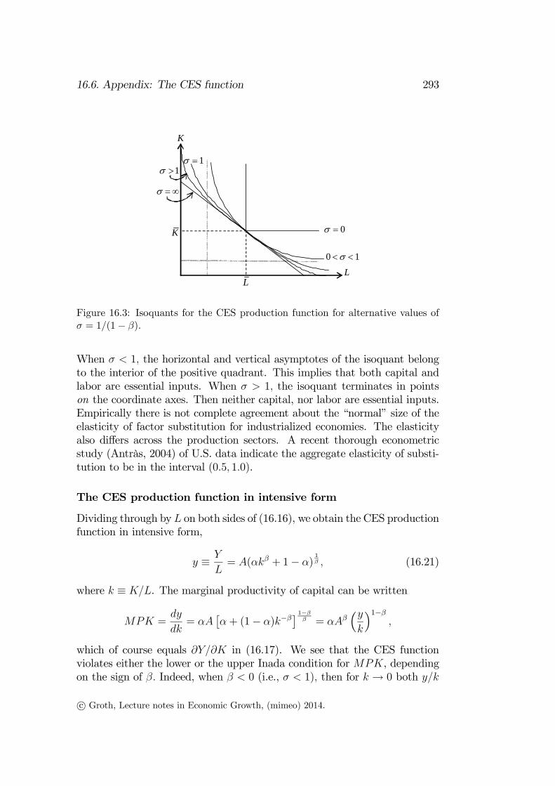
Figure 16.3 depicts isoquants for alternative CES production functions

and their limiting cases. In the Cobb-Douglas case, = 1 the horizontal

and vertical asymptotes of the isoquant coincide with the coordinate axes.

20For proofs of this and the further claims below, see Appendix E of Chapter 4 in Groth

(2013).



K

1

L

0 K

1

0 1

L

Figure 16.3: Isoquants for the CES production function for alternative values of

= 1(1− ).

When 1 the horizontal and vertical asymptotes of the isoquant belong

to the interior of the positive quadrant. This implies that both capital and

labor are essential inputs. When 1 the isoquant terminates in points

on the coordinate axes. Then neither capital, nor labor are essential inputs.

Empirically there is not complete agreement about the “normal” size of the

elasticity of factor substitution for industrialized economies. The elasticity

also differs across the production sectors. A recent thorough econometric

study (Antràs, 2004) of U.S. data indicate the aggregate elasticity of substi-

tution to be in the interval (05 10).

The CES production function in intensive form

Dividing through by on both sides of (16.16), we obtain the CES production

function in intensive form,

≡

= ( + 1− )

1 (16.21)

where ≡ . The marginal productivity of capital can be written

=

=

£+ (1− )−

¤ 1− =

³

´1−

which of course equals in (16.17). We see that the CES function

violates either the lower or the upper Inada condition for , depending

on the sign of Indeed, when 0 (i.e., 1) then for → 0 both


294


GROWTH

y

k

y

0 (0 1)

1/A

k 0 ( 1)

1/A

1/(1 )A

1/(1 )A

Figure 16.4: The CES production function for 1 (left panel) and 1 (right

panel).

and approach an upper bound equal to 1 ∞ thus violating the

lower Inada condition for (see the right-hand panel of Figure 2.3 in

Chapter 2). It is also noteworthy that in this case, for →∞, approachesan upper bound equal to (1 − )1 ∞. These features reflect the lowdegree of substitutability when 0

When instead 0 there is a high degree of substitutability ( 1).

Then, for →∞ both and → 1 0 thus violating the upper

Inada condition for (see the right-hand panel of Figure 16.4). It is

also noteworthy that for → 0, approaches a positive lower bound equal

to (1− )1 0. Thus, in this case capital is not essential. At the same

time → ∞ for → 0 (so the lower Inada condition for the marginal

productivity of capital holds).

The marginal productivity of labor is

=

= (1− )( + 1− )(1−) ≡ ()

from (16.17).

Since (16.16) is symmetric in and we get a series of symmetric results

by considering output per unit of capital as ≡ = £+ (1− )()

¤1

In total, therefore, when there is low substitutability ( 0) for fixed input

of either of the production factors, there is an upper bound for how much

an unlimited input of the other production factor can increase output. And

when there is high substitutability ( 0) there is no such bound and an

unlimited input of either production factor take output to infinity.

The Cobb-Douglas case, i.e., the limiting case for → 0 constitutes in

several respects an intermediate case in that all four Inada conditions are

satisfied and we have → 0 for → 0 and →∞ for →∞



Generalizations

The CES production function considered above has CRS. By adding an elas-

ticity of scale parameter, , we get the generalized form

= £ + (1− )

¤ 0 (16.22)

In this form the CES function is homogeneous of degree For 0 1

there are DRS, for = 1 CRS, and for 1 IRS. If 6= 1 it may be

convenient to consider ≡ 1 = 1£ + (1− )

¤1and ≡

= 1( + 1− )1

The elasticity of substitution between and is = 1(1−) whateverthe value of So including the limiting cases as well as non-constant returns

to scale in the “family” of production functions with constant elasticity of

substitution, we have the simple classification displayed in Table 16.1.

Table 16.1 The family of production functions

with constant elasticity of substitution.

= 0 0 1 = 1 1

Leontief CES Cobb-Douglas CES

Note that only for ≤ 1 is (16.22) a neoclassical production function.This is because, when 1 the conditions 0 and 0 do not

hold everywhere.

We may generalize further by assuming there are inputs, in the amounts

12 Then the CES production function takes the form

= £11

+ 22 +

¤ 0 for all

X

= 1 0

(16.23)

In analogy with (16.18), for an -factor production function the partial elas-

ticity of substitution between factor and factor is defined as

=

()

|=

where it is understood that not only the output level but also all , 6= , ,

are kept constant. Note that = In the CES case considered in (16.23),

all the partial elasticities of substitution take the same value, 1(1− )


296


GROWTH

16.7 Literature

Antràs, 2004, ...

Arrow, K. J., et al., 1961, ...

Arrow, K. J., P. Dasgupta, L. Goulder, G. Daily, P. Ehrlich, G. Heal, S.

Levin, K.-G. Mäler, S. Schneider, D. Starrett, and B. Walker, 2004,

Are we consuming too much?, J. of Economic Perspectives 18, no. 3,

147-172.

Arrow, K.J, P. Dasgupta, L. Goulder, K. Mumford, and K.L.L. Oleson,

2012, Sustainability and the measurement of wealth, Environment and

Development Economics 17, no. 3, 317—353.

Brock, W. A., and M. Scott Taylor, 2005. Economic Growth and the Envi-

ronment: A review of Theory and Empirics. In: Handbook of Economic

Growth, vol. 1.B, ed. by ...

Brundtland Commission, 1987, ...

Brynjolfsson, E., and A. McAfee, 2014, The Second Machine Age, Norton.

Dasgupta, P., 1993, Natural resources in an age of substitutability. In:

Handbook of Natural Resource and Energy Economics, vol. 3, ed. by

A. V. Kneese and J. L. Sweeney, Elsevier: Amsterdam, 1111-1130.

Dasgupta, P., and G. M. Heal, 1974, The optimal depletion of exhaustible

resources, Review of Economic Studies, vol. 41, Symposium, 3-28.

Fagnart, J.-F., and M. Germain, 2011, Quantitative vs. qualitative growth

with recyclable resources, Ecological Economics, vol. 70, 929-941.

Gordon, R.J., 2012, Is US economic growth over? Faltering innovation

confronts the six headwinds, NBER WP no. 18315.

Grossman, G.M., and A.B. Krueger, 1995, , QJE, vol. 90 (2).

Groth, C., 2007, A New-Growth Perspective on Non-renewable Resources.

In: Sustainable Resource Use and Economic Dynamics, ed. by L.

Bretschger and S. Smulders, Springer Verlag: Dordrecht (available at

the course website).

Groth, C., 2013, Lecture notes in macroeconomics (mimeo), Depart. of

Economics, University of Copenhagen.


16.7. Literature 297

Handbook of Natural Resource and Energy Economics, vol. III, ed. by A.

V. Kneese and J. L. Sweeney, Elsevier: Amsterdam, 1993.

Hamilton, K., 2012, Comments on Arrow et al., ‘Sustainability and the

measurement of wealth’, Environment and Development Economics 17,

no. 3, 356 - 361.

Heal, G., 1998. Valuing the Future. Economic Theory and Sustainability.

Columbia University Press: New York.

Jones, C., 2002, Introduction to Economic Growth, 2. ed., W.W. Norton:

New York.

Lind, S., og P. Schou, P., 2013, Ægte opsparing, Arbejdspapir 2013:1, De

Økonomiske Råds Sekretariat, København.

Meadows, D. H., and others, 1972, The Limits to Growth, Universe Books:

New York.

Smil, V., 2003, Energy at the crossroads. Global perspectives and uncertain-

ties, Cambridge Mass.: MIT Press.

Smulders, S., 1995, Entropy, environment, and endogenous growth, Inter-

national Tax and Public Finance, vol. 2, 319-340.

Smulders, S., 1999,

Smulders, S., 2012, An arrow in the Achilles’ heel of sustainability and

wealth accounting, Environment and Development Economics 17, no.

3, 368-372.

Solow, R.M., 1974, Review of Economic Studies, vol. 41,

Symposium.

Solow, R.M., 2012, A few comments on ‘Sustainability and the measurement

of wealth, Environment and Development Economics 17, no. 3, 354-

355.

Squires and Vestergaard, 2011,

Sterner, T., 2008, The costs and benefits of climate policy: The impact of

the discount rate and changing relative prices. Lecture at Miljøøkonomisk

konference 2008 in Skodsborg, see http://www.dors.dk/graphics/Synkron-

Library/Konference%202008/

Keynote/Sterner_Copenhagen_SEPT08.pdf


298


GROWTH

Stiglitz, J., 1994, Review of Economic Studies, vol. 41,

Symposium.

Stiglitz, J., A. Sen, and J.-P. Fitoussi, 2009, Report by the Commission

on the Measurement of Economic Performance and Social Progress,

www.stiglitz-sen-fitoussi.fr.

Stiglitz, J., A. Sen, and J.-P. Fitoussi, 2010, Mismeasuring Our Lives. Why

the GDP Doesn’t Add Up, The New Press: New York.

Weitzman, M., 2001, A contribution to the theory of welfare accounting,

Scandinavian J. of Economics 103 (1), 1-23.

Weitzman, M., 2003, Income, Wealth, and the Maximum Principle, Harvard

Univ. Press: Cambridge (Mass.).

van Kooten, G. C., and E. H. Bulte, 2000. The Economics of Nature.

Managing Biological Assets. Blackwell: Oxford.


Date post:	09-Mar-2018
Category:	Documents
Upload:	vannhu
View:	224 times
Download:	6 times

Chapter 16 Natural resources and economic growth - kuweb.econ.ku.dk/okocg/VV/VV-2014/Lectures and...

Documents