Chapter 19

Applications of Standard Electrode Potentials

Many analytical techniques have been used to measure the chemical and physical properties of chlorophyll to explore its role in photosynthesis. The redox titration of chlorophyll with other standard redox couples reveals the oxidation/ reduction properties of the molecule that help explain the photophysics of the complex process that green plants use to oxidize water to molecular oxygen.

This composite satellite image displays areas on the surface of the Earth where chlorophyll-bearing plants are located. Chlorophyll, which is one of nature’s most important biomolecules, is a member of a class of compounds called porphyrins. This class also includes hemoglobin and cytochrome c, which is discussed in Feature 19-1.

2

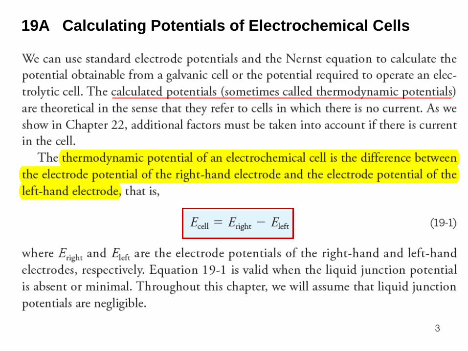
19A Calculating Potentials of Electrochemical Cells

3

Gustav Robert Kirchhoff (1824-1877) was a German physicist who made many important contributions to physics and chemistry. In addition to his work in spectroscopy, he is known for Kirchhoff’s laws of current and voltage in electrical circuits. These laws can be summarized by the following equations: Σ I = 0 and Σ E = 0. These equations state that the sum of the currents into any circuit point (node) is zero and the sum of the potential differences around any circuit loop is zero.

4

Example 19-1 Calculating potentials of electrochemical cells Ecell = Eright – Eleft

Ex. Cu Cu2+(0.0200M) Ag+(0.0200M) Ag

Cu (s) + 2Ag+ = Cu2+(aq) + 2Ag(s)

Ag+ + e Ag(s) Eo = + 0.799 V

Cu2+ + 2e Cu(s) Eo = + 0.337 V

2Ag+ + 2e 2Ag(s) Eo = + 0.799 V E = 0.799 – (0.05916/1) log (1/0.0200) = 0.6984 V

Cu2+ + 2e Cu(s) Eo = + 0.337 V E = 0.337 – (0.05916/2) log (1/0.0200) = 0.2867V

Cu (s) + 2Ag+ Cu2+(aq) + 2Ag(s)

Eocell = + 0.799 V – (+ 0.337 V) Ecell = Eright – Eleft = 0.6984 – 0.2864

= + 0.462 V = + 0.412 V

∆G = – nFE = – 2 ×96485 C × 0.412 V = 79,503 J (18.99 kcal)

5

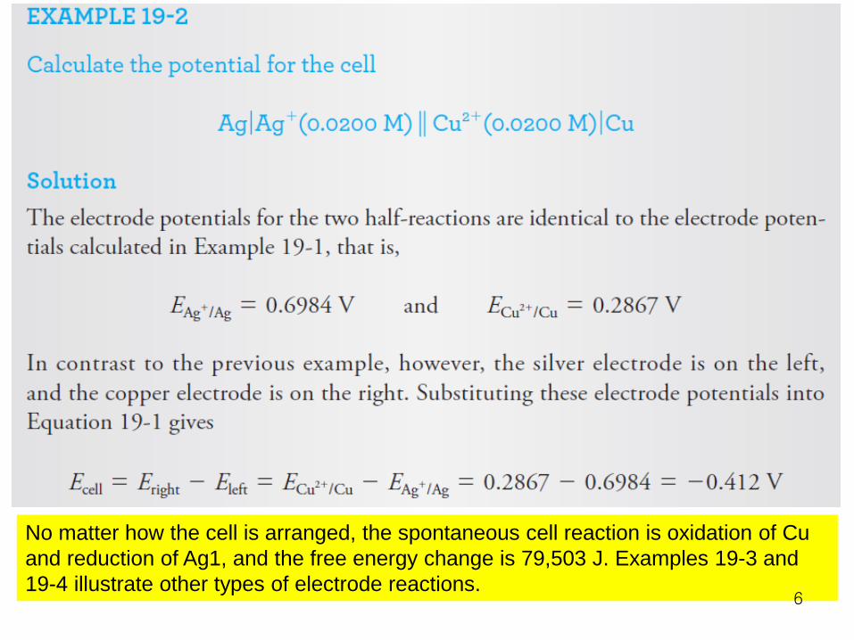
No matter how the cell is arranged, the spontaneous cell reaction is oxidation of Cu and reduction of Ag1, and the free energy change is 79,503 J. Examples 19-3 and 19-4 illustrate other types of electrode reactions.

6

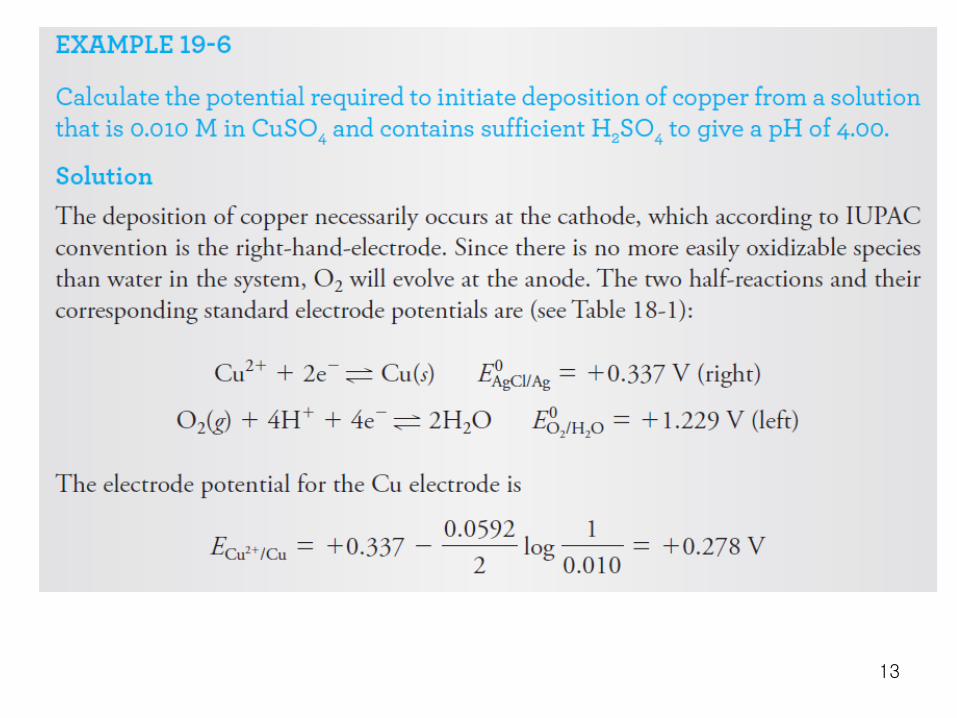
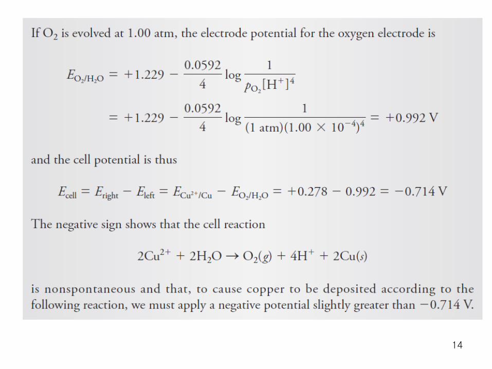
Example 19-3 Calculate the potential of the following cell and indicate the reaction that would occur spontaneously if the cell were short-circuited. Pt U4+(0.200M), UO2

2+(0.0150M), H+(0.300M) Fe2+(0.0100M), Fe3+ (0.0250M) Pt

Figure 19-1 Cell for Example 19-3. 7

The two half-reactions are Fe3+ + e_ Fe2+ Eo = + 0.771V UO2

2+ + 4H+ + 2e- U4+ + 2H2O Eo = + 0.334V The electrode potential for the right-hand electrode is Eright = 0.771 – 0.05916 log [Fe 2+]/[Fe 3+] = 0.771 – 0.05916 log 0.0100/0.0250 = 0.771 – (– 0.0236) = 0.7946 V The electrode potential for the left-hand electrode is ELeft = 0.334 – (0.0592 / 2) log [U4+ ] / [UO2

2+][ H+]4

= 0.334 – (0.0592 / 2) log 0.200 / (0.0150) (0.0300) 4

= 0.334 – 0.2136 = 0.1204 V And E cell = E right – E left = 0.7946 – 0.2136 = 0.674V The positive sign means that the spontaneous reaction is the oxidation of U4+ on the left and the reduction of Fe 3+ on the right, or U4+ +2 Fe 3+ + 2H2O UO2

2+ +Fe 2+ + 4H+

8

Example 19-4 Calculate the cell potential for Ag AgCl (sat’d), HCl (0.0200M) H2(0.800atm ), Pt

Figure 19-2 Cell without liquid junction for example 19-4

Note that this cell does not require two compartments (nor a salt bridge) because molecular H2 has little tendency to react directly with the low concentration of Ag+ in the electrolyte solution. This is an example of a cell without liquid junction.

9

Solutions The two half- reactions and their corresponding standard electrode potentials are 2H+ + 2e - H2 Eo

H+/H2 = 0.000V AgCl(s) + e - Ag (s) + Cl– Eo

AgCl/Ag = 0.222V The two electrode potentials are Eright = 0.000 – (0.0592/2)log pH2 / [H+]2

= – (0.0592/2) log 0.800 / (0.0200) 3 = – 0.0977 V Eleft = 0.222 – 0.0592log [Cl-] = 0.222 – 0.0592 log 0.0200 = 0.3226V The cell potential is thus E cell = E right – E left = -0.0977 – 0.3226 = – 0.420V The negative sign indicates that the cell reaction as considered 2H+ + 2 Ag(s) H2 + 2AgCl(s) is nonspontaneous. To get this reaction to occur, we would have to apply an external voltage and construct an electrolytic cell.

10

Example 19-5

Calculate the potential for the following cell using (a) concentration and (b) activities:

Zn ZnSO4(5.00 ×10–4 M), PbSO4 (sat’d) Pb

(a) [SO42–] = CZnSO4 = 5.00 ×10–4

PbSO4(s) + 2e Pb (s) + SO42– Eo

= – 0.350 V

Zn2+ + 2e Zn (s) Eo = – 0.763 V

Eright = Eo – (0.05916 / 2) log [SO4

2–] = – 0.350 – (0.05916 / 2) log (5.00 ×10–4)

= – 0.252 V

Eleft = Eo – (0.05916 / 2) log (1 / [Zn2+]

= – 0.763 – (0.05916 / 2) log {1 / (5.00 ×10–4)} = – 0.860 V

Ecell = Eright – Eleft = – 0.252 – (– 0.860) = 0.608 V

11

(b) Ionic strength for 5.00 ×10–4 M ZnSO4 :

µ = (1/2) {(5.00 ×10–4) ×(+2)2 + (5.00 ×10–4) ×(– 2)2 } = 2.00 ×10–3

Debye-Huckel Eq. : – log γ = (0.51 Z2 √µ ) / ( 1+ 3.3α √µ )

α SO42– = 0.4 nm , α Zn2+ = 0.4 nm

∴ γ SO42– = 0.820, γ Zn2+ = 0.825

Activity = γ [C]

Eright = Eo – (0.05916 / 2) log {γ SO42– [SO4

2–] }

= – 0.350 – (0.05916 / 2) log (0.820 × 5.00 ×10–4) = – 0.250 V

Eleft = Eo – (0.05916 / 2) log {1 / (γ Zn2+ [Zn2+])}

= – 0.763 – (0.05916 / 2) log {1 / (0.825 × 5.00 ×10–4)} = – 0.863 V

Ecell = Eright – Eleft = – 0.250 – (– 0.863) = 0.613 V

12

13

14

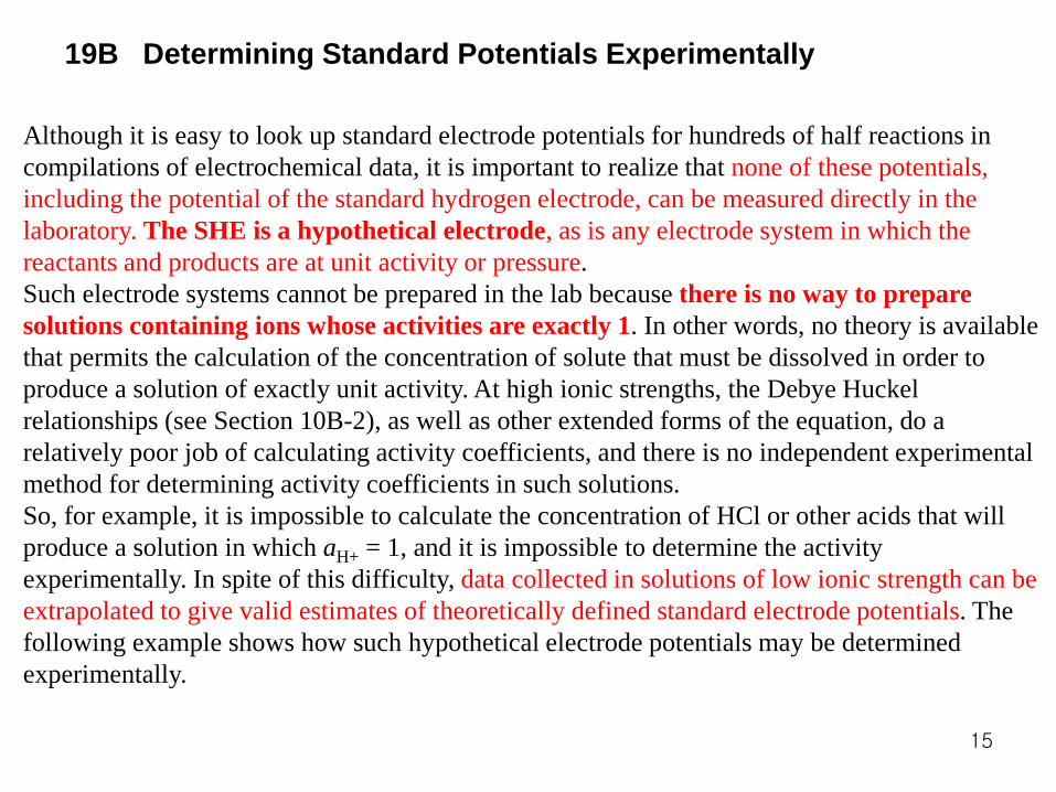
19B Determining Standard Potentials Experimentally

Although it is easy to look up standard electrode potentials for hundreds of half reactions in compilations of electrochemical data, it is important to realize that none of these potentials, including the potential of the standard hydrogen electrode, can be measured directly in the laboratory. The SHE is a hypothetical electrode, as is any electrode system in which the reactants and products are at unit activity or pressure. Such electrode systems cannot be prepared in the lab because there is no way to prepare solutions containing ions whose activities are exactly 1. In other words, no theory is available that permits the calculation of the concentration of solute that must be dissolved in order to produce a solution of exactly unit activity. At high ionic strengths, the Debye Huckel relationships (see Section 10B-2), as well as other extended forms of the equation, do a relatively poor job of calculating activity coefficients, and there is no independent experimental method for determining activity coefficients in such solutions. So, for example, it is impossible to calculate the concentration of HCl or other acids that will produce a solution in which aH+ = 1, and it is impossible to determine the activity experimentally. In spite of this difficulty, data collected in solutions of low ionic strength can be extrapolated to give valid estimates of theoretically defined standard electrode potentials. The following example shows how such hypothetical electrode potentials may be determined experimentally.

15

16

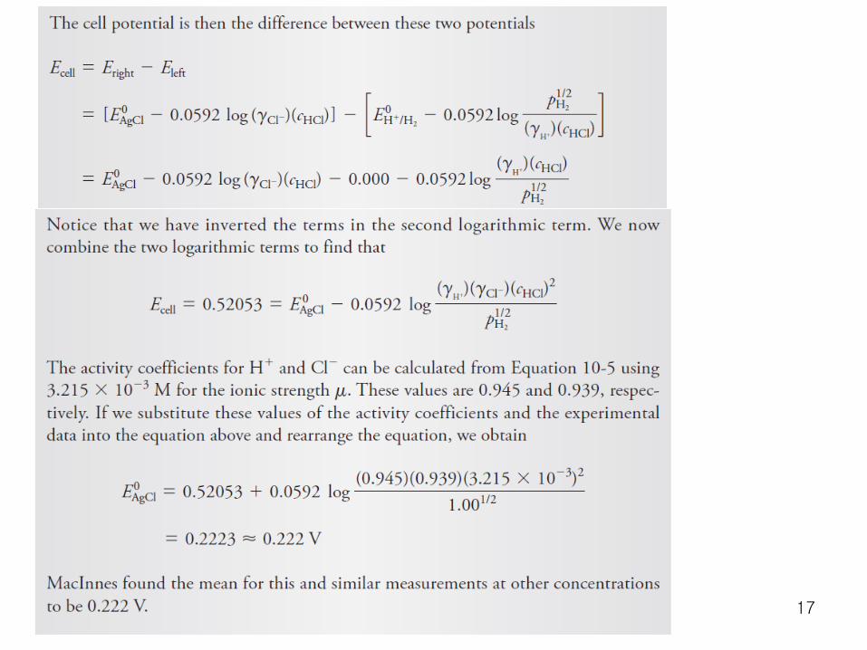
17

18

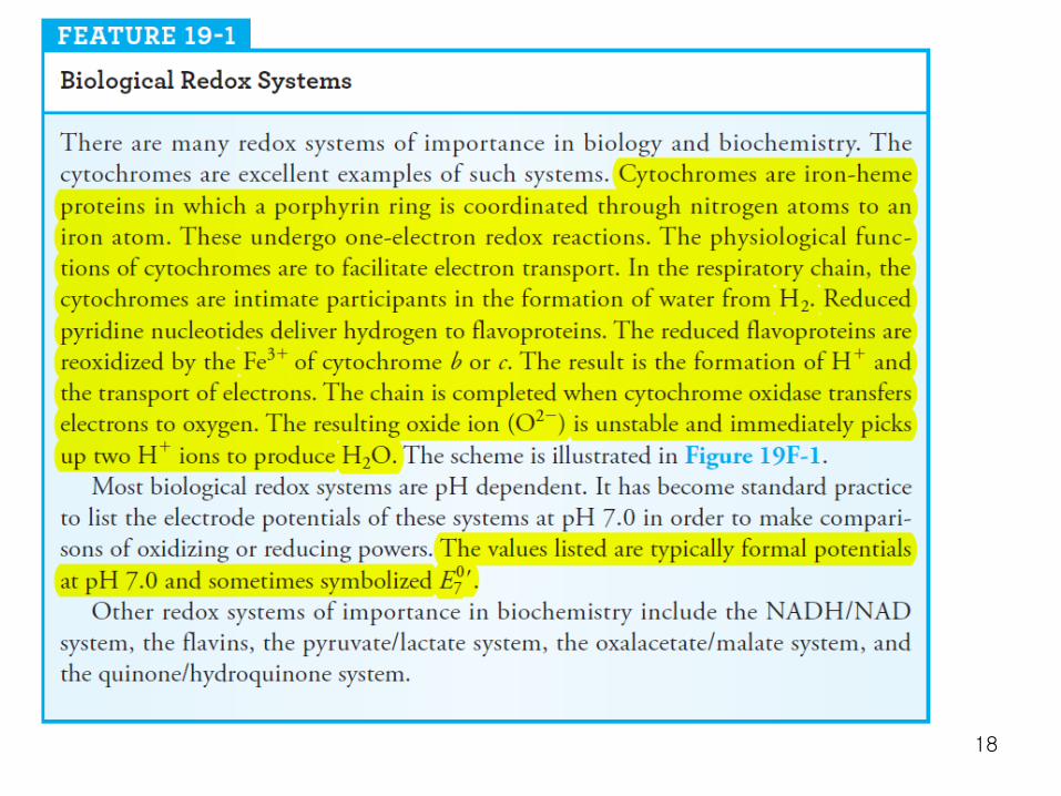
Figure 19F-1 Redox systems in the respiratory chain. P = phosphate ion. (From P. Karlson, Introduction to Modern Biochemistry, New York: Academic Press, 1963. With permission.)

19

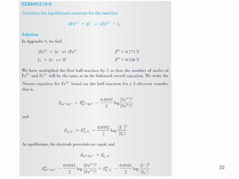
19-C Calculation Redox Equilibrium Constant

Cu Cu2+(x M) Ag+(y M) Ag

Cu (s) + 2Ag+ Cu2+(aq) + 2Ag(s) (19-4)

Keq = [Cu2+] / [Ag+]2 2Ag+ + 2e 2Ag(s) Eo = + 0.799 V

Cu2+ + 2e Cu(s) Eo = + 0.337 V

Ecell = Eright – Eleft = EAg – ECu = 0 or Eright = Eleft = EAg = ECu Eo

Ag – (0.05916/2) log (1/[Ag+]2) = EoCu – (0.05916/2) log (1/[Cu2+])

EoAg – Eo

Cu = (0.05916/2) log (1/[Ag+]2) – (0.05916/2) log (1/[Cu2+])

EoAg – Eo

Cu = (0.05916/2) log (1/[Ag+]2) + (0.05916/2) log ([Cu2+]/1)

2 (EoAg – Eo

Cu ) / 0.05916 = log ([Cu2+]/[Ag+]2 ) = log Keq

ln Keq = –∆Go/RT= – nFEocell / RT

ln Keq = – nEocell / 0.05916 = – n (Eo

right – Eoleft ) / 0.05916 <At 25oC >

20

21

22

23

24

Note that the product ab is the total number of electrons gained in the reduction (and lost in the oxidation) represented by the balanced redox equation. Thus, if a = b, it is not necessary to multiply the half-reactions by a and b. If a = b = n, the equilibrium constant is determined from 25

26

27

19D Constructing Redox Titration Curves 19D-1 Electrode Potentials during Redox Titrations Consider the redox titration of iron(II) with a standard solution of cerium(IV). Titration reaction:

This reaction is rapid and reversible so that the system is at equilibrium at all times throughout the titration. Consequently, the electrode potentials for the two half-reactions are always identical (Equation 19-6).

If a redox indicator has been added to this solution, the ratio of the concentrations of its oxidized and reduced forms must adjust so that the electrode potential for the indicator, EIn, is also equal to the system potential.

We can calculate the electrode potential of a system from standard potential data. Thus, for the reaction under consideration, the titration mixture is treated as if it were part of the hypothetical cell

28

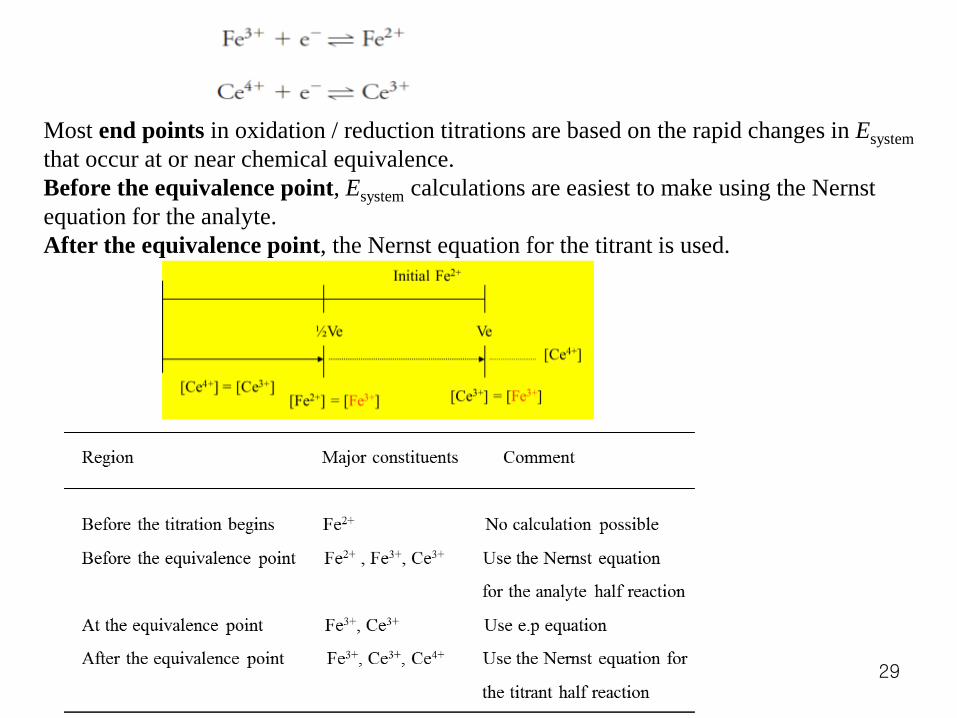
Most end points in oxidation / reduction titrations are based on the rapid changes in Esystem that occur at or near chemical equivalence. Before the equivalence point, Esystem calculations are easiest to make using the Nernst equation for the analyte. After the equivalence point, the Nernst equation for the titrant is used.

29

Equivalence-Point Potentials Equivalence point potentials are easily obtained by taking advantage of the fact that the two reactant species and the two product species have known concentration ratios at chemical equivalence. At the equivalence point in the titration of iron(II) with cerium(IV), the potential of the system is given by both and

30

31

32

19D-2 The Titration Curve

33

34

35

Before the equivalence point (amount Fe2+ remaining) = (amount Fe2+ initial) – (amount Ce4+ added ≡ amount Fe2+ used)

(amount Fe3+ produced) = (amount Fe2+ used)

[Fe2+] = amount Fe2+ (mmol) / vol(ml), [Fe3+] = amount Fe3+ (mmol) / vol(ml)

36

Table 19-2.

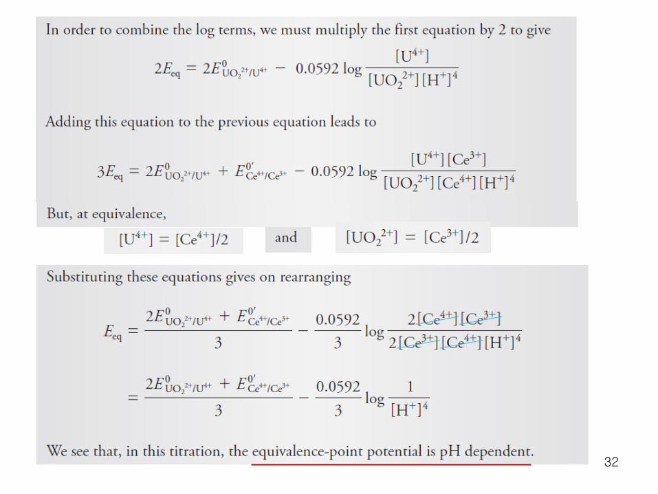
At the equivalence point

[Ce3+] = [Fe3+]

[Ce4+] = [Fe2+]

Eeq = EoCe4+ – 0.05916 log[Ce3+]/ [Ce4+]

Eeq = EoFe3+ – 0.05916 log[Fe2+]/ [Fe3+]

2Eeq = EoCe4+ + Eo

Fe3+– 0.05916 log[Ce3+]/ [Ce4+] – 0.05916 log[Fe2+]/ [Fe3+]

= EoCe4+ + Eo

Fe3+– 0.05916 log[Ce3+] [Fe2+] / [Ce4+] [Fe3+]

= EoCe4+ + Eo

Fe3+

Eeq = (EoCe4+ + Eo

Fe3+ ) / 2

E(cell) = Eright – ESHE 37

38

After the equivalence point

[Fe2+] = 0

E(cell) = Eright – ESHE

amount Ce4+ remaining = amount Ce4+ added – amount Ce4+ used

= amount Ce4+ added – (amount Fe2+ initial × reacting ratio )

39

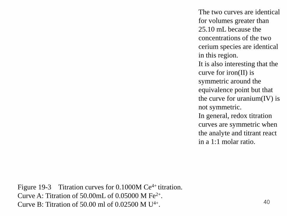
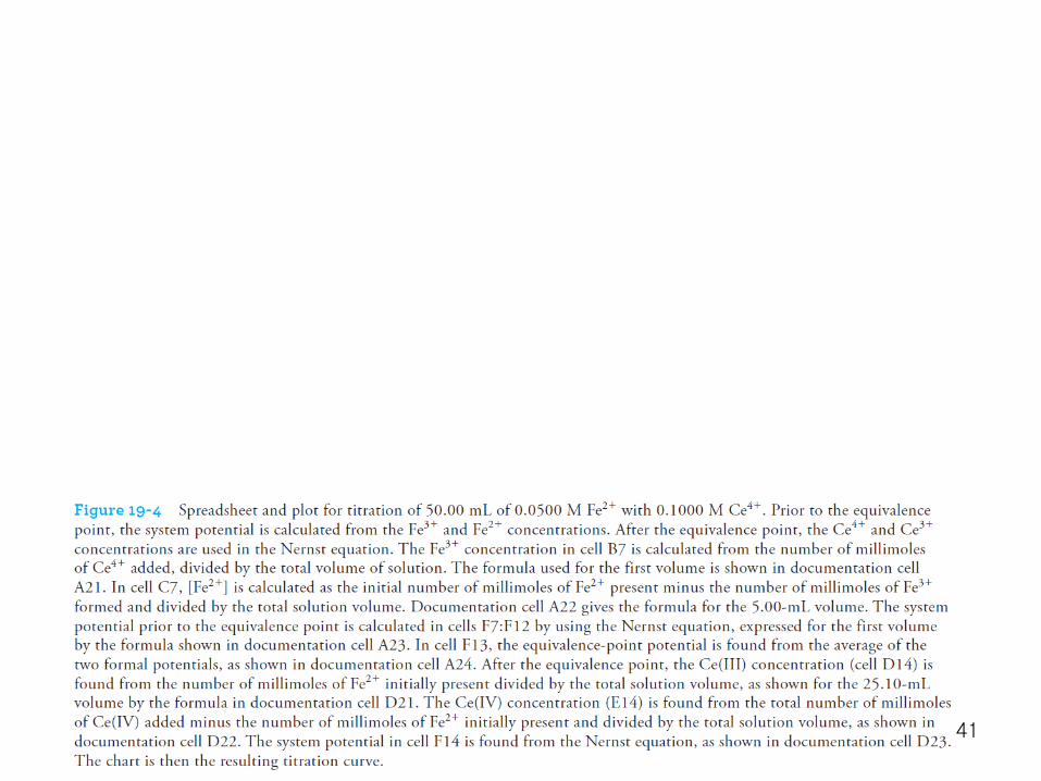
Figure 19-3 Titration curves for 0.1000M Ce4+ titration. Curve A: Titration of 50.00mL of 0.05000 M Fe2+. Curve B: Titration of 50.00 ml of 0.02500 M U4+.

The two curves are identical for volumes greater than 25.10 mL because the concentrations of the two cerium species are identical in this region. It is also interesting that the curve for iron(II) is symmetric around the equivalence point but that the curve for uranium(IV) is not symmetric. In general, redox titration curves are symmetric when the analyte and titrant react in a 1:1 molar ratio.

40

41

42

43

44

45

46

47

48

49

50

51

52

19D-3 Effect of Variables on Redox Titration Curves

1) concentration

2) completeness of reaction V(ml)

E(V) concentrated

diluted

V(ml)

E(V) Higher Eo titrant

Lower Eo titrant

53

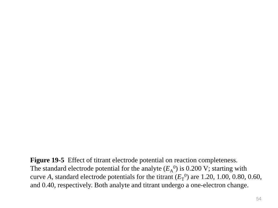
Figure 19-5 Effect of titrant electrode potential on reaction completeness. The standard electrode potential for the analyte (EA

0) is 0.200 V; starting with curve A, standard electrode potentials for the titrant (ET

0) are 1.20, 1.00, 0.80, 0.60, and 0.40, respectively. Both analyte and titrant undergo a one-electron change.

54

55

19E Oxidation/Reduction Indicators 19E-1 General Redox Indicators

56

57

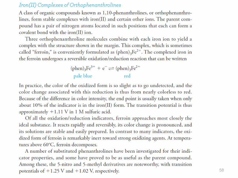
58

59

Starch-Iodine complex

Starch solution(05~ 1%) is not redox indicator.

The active fraction of starch is amylose, a polymer of the sugar α-D-glucose ( 1,4 bond).

The polymer exists as a coiled helix into which small molecules can fit.

In the presence of starch and I–, iodine molecules form long chains of I5– ions

that occupy the center of the amylose helix.

••••[I I I I I]– ••••[I I I I I]– ••••

Visible absorption by the I5– chain bound within the helix gives rise to the

characteristic starch-iodine color.

60

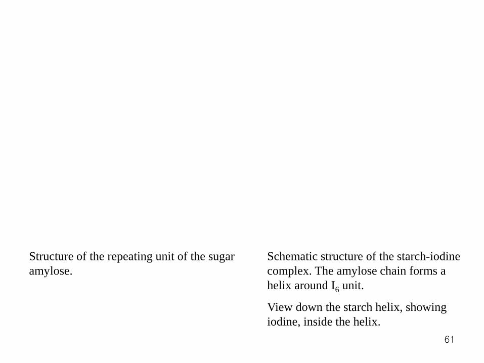
Structure of the repeating unit of the sugar amylose.

Schematic structure of the starch-iodine complex. The amylose chain forms a helix around I6 unit.

View down the starch helix, showing iodine, inside the helix.

61

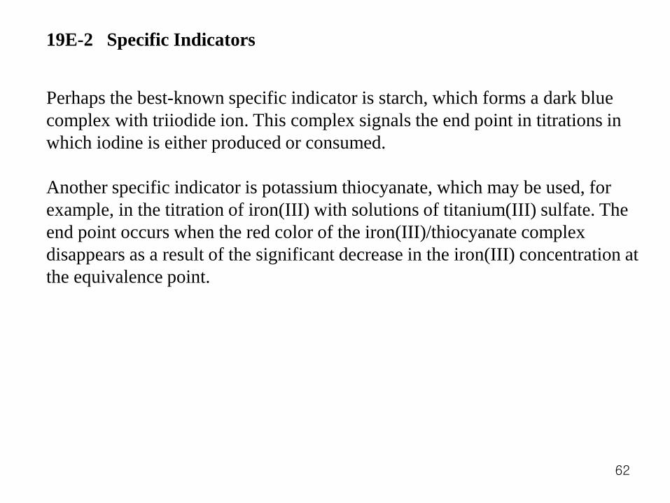
19E-2 Specific Indicators

Perhaps the best-known specific indicator is starch, which forms a dark blue complex with triiodide ion. This complex signals the end point in titrations in which iodine is either produced or consumed. Another specific indicator is potassium thiocyanate, which may be used, for example, in the titration of iron(III) with solutions of titanium(III) sulfate. The end point occurs when the red color of the iron(III)/thiocyanate complex disappears as a result of the significant decrease in the iron(III) concentration at the equivalence point.

62

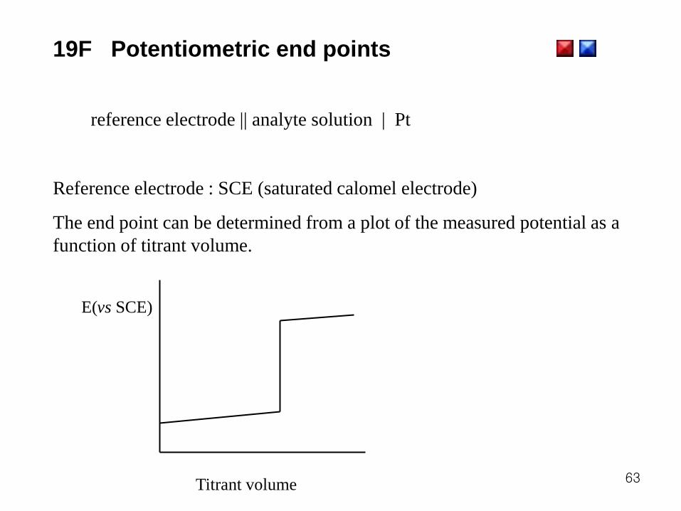
19F Potentiometric end points

reference electrode || analyte solution | Pt

Reference electrode : SCE (saturated calomel electrode)

The end point can be determined from a plot of the measured potential as a function of titrant volume.

E( vs SCE)

Titrant volume 63

Summary

potentials of electrochemical cells

Standard potential

SHE

Formal potentials

Redox equilibrium constant

Redox titration curve

Redox indicators

Starch-iodine complex

Potentiometric end point, SCE

64