There are four fundamental types of properties of a hydrocarbon reservoirthat control its initial contents, behavior, production potential, and henceits reserves.1. The rock properties of porosity, permeability, and compressibility, which
are all dependent on solid grain/particle arrangements and packing.2. The wettability properties, capillary pressure, phase saturation, and rela-
tive permeability, which are dependent on interfacial forces between thesolid and the water and hydrocarbon phases.
3. The initial ingress of hydrocarbons into the reservoir trap and the ther-modynamics of the resulting reservoir mixture composition.
4. Reservoir fluid properties, phase compositions, behavior of the phaseswith pressure, phase density, and viscosity.In this chapter we look at the basics of each of these properties, and also
consider how they are estimated.
2.2 POROSITY
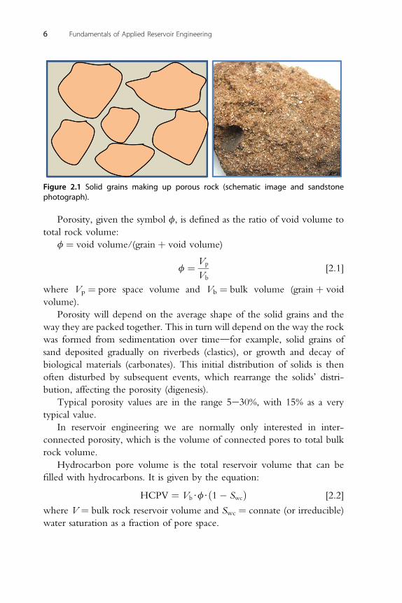
2.2.1 BasicsPorous rock is the essential feature of hydrocarbon reservoirs. Oil or gas (orboth) is generated from source layers, migrates upwards by displacing waterand is trapped by overlying layers that will not allow hydrocarbons to movefurther upwards. Porous material in hydrocarbon reservoirs can be dividedinto clastics and carbonates. Clastics such as sandstone are composed of smallgrains normally deposited in riverbeds over long periods of time andcovered and compressed over geological periods (Fig. 2.1). Carbonates(various calcium carbonate minerals) are typically generated by biologicalprocesses and again compressed by overlying material over long periods oftime. Roughly 60% of conventional oil and gas resources occur in clasticsand 40% in carbonates.
Fundamentals of Applied Reservoir EngineeringISBN 978-0-08-101019-8http://dx.doi.org/10.1016/B978-0-08-101019-8.00002-8
Porosity, given the symbol f, is defined as the ratio of void volume tototal rock volume:
f ¼ void volume/(grain þ void volume)
f ¼ Vp
Vb[2.1]
where Vp ¼ pore space volume and Vb ¼ bulk volume (grain þ voidvolume).
Porosity will depend on the average shape of the solid grains and theway they are packed together. This in turn will depend on the way the rockwas formed from sedimentation over timedfor example, solid grains ofsand deposited gradually on riverbeds (clastics), or growth and decay ofbiological materials (carbonates). This initial distribution of solids is thenoften disturbed by subsequent events, which rearrange the solids’ distri-bution, affecting the porosity (digenesis).
Typical porosity values are in the range 5e30%, with 15% as a verytypical value.
In reservoir engineering we are normally only interested in inter-connected porosity, which is the volume of connected pores to total bulkrock volume.
Hydrocarbon pore volume is the total reservoir volume that can befilled with hydrocarbons. It is given by the equation:
HCPV ¼ Vb$f$ð1� SwcÞ [2.2]
where V ¼ bulk rock reservoir volume and Swc ¼ connate (or irreducible)water saturation as a fraction of pore space.
Figure 2.1 Solid grains making up porous rock (schematic image and sandstonephotograph).
6 Fundamentals of Applied Reservoir Engineering
As pressure decreases with hydrocarbon production, rock particles willtend to pack closer together so that porosity will decrease somewhat as afunction of pressure. This is known as rock compressibility (cr):
cr ¼ � 1Vp
vVp
vP[2.3]
where Vp ¼ Vb$f ¼ pore volume.Porosity of real rocks is often (in fact normally) very heterogeneous,
depending on the lithology of the rockdwhich is typically variable evenover quite short distances. Certainly, layer by layer and aerially within thereservoir porosity will vary significantly.
Also the geometry of the pore space is very variable, so that two samplesof porous material, even if they have the same porosity, can have verydifferent resistance to fluid flow. We discuss this in detail later.
2.2.2 Measurement of PorosityPorosity is measured in two ways, from either wire line logs or laboratorymeasurement on core.
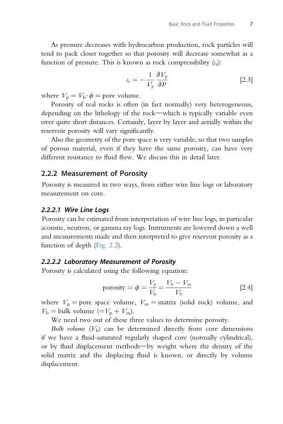
2.2.2.1 Wire Line LogsPorosity can be estimated from interpretation of wire line logs, in particularacoustic, neutron, or gamma ray logs. Instruments are lowered down a welland measurements made and then interpreted to give reservoir porosity as afunction of depth (Fig. 2.2).
2.2.2.2 Laboratory Measurement of PorosityPorosity is calculated using the following equation:
porosity ¼ f ¼ Vp
Vb¼ Vb � Vm
Vb[2.4]
where Vp ¼ pore space volume, Vm ¼ matrix (solid rock) volume, andVb ¼ bulk volume (¼Vp þ Vm).
We need two out of these three values to determine porosity.Bulk volume (Vb) can be determined directly from core dimensions
if we have a fluid-saturated regularly shaped core (normally cylindrical),or by fluid displacement methodsdby weight where the density of thesolid matrix and the displacing fluid is known, or directly by volumedisplacement.
Basic Rock and Fluid Properties 7
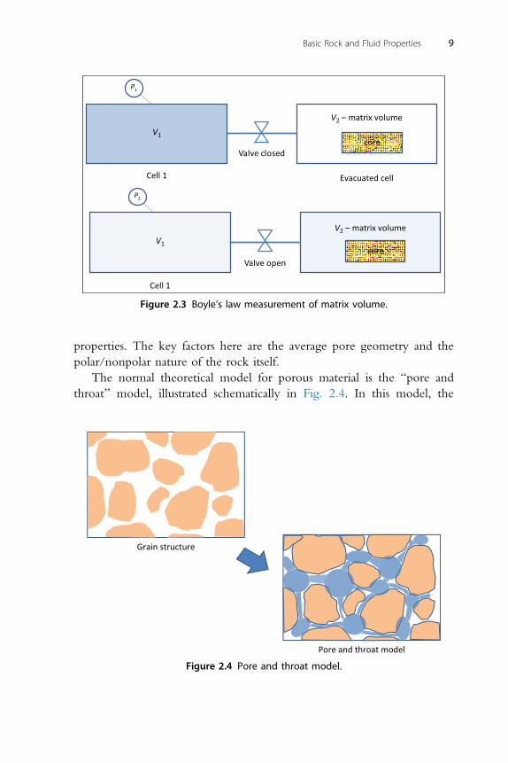
Matrix volume (Vm) can be calculated from the mass of a dry sampledivided by the matrix density. It is also possible to crush the dry solid andmeasure its volume by displacement, but this will give total porosity ratherthan effective (interconnected) porosity. A gas expansion method can beused: gas in a cell at known pressure is allowed to expand into a second cellcontaining core where all gas present has been evacuated. The final (lower)pressure is then used to calculate the matrix volume present in the secondcell using Boyle’s law (Fig. 2.3). This method can be very accurate, espe-cially for low-porosity rock.
Boyle’s law: P1V1 ¼ P2V2 (assuming gas deviation factor Z can beignored at relatively low pressures) can now be used.
Pore space volume (Vp) can also be determined using gas expansionmethods.
2.2.3 Variable Nature of PorosityAs discussed above, porosity is very variable in its nature, changing overquite small distances within a reservoir; and even if two samples have thesame porosity, it does not mean that they will have the same absolutepermeability or the same wettability characteristics, which in turn meansthat they can have very different capillary pressure and relative permeability
Figure 2.2 Wire line well loggingdschematic and example log.
8 Fundamentals of Applied Reservoir Engineering
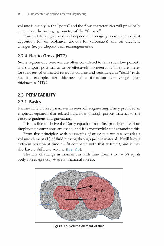
properties. The key factors here are the average pore geometry and thepolar/nonpolar nature of the rock itself.
The normal theoretical model for porous material is the “pore andthroat” model, illustrated schematically in Fig. 2.4. In this model, the
V1
V2 – matrix volume
V2 – matrix volume
core
P1
Cell 1 Evacuated cell
V1core
P2
Cell 1
Valve closed
Valve open
Figure 2.3 Boyle’s law measurement of matrix volume.
Grain structure
Pore and throat model
Figure 2.4 Pore and throat model.
Basic Rock and Fluid Properties 9
volume is mainly in the “pores” and the flow characteristics will principallydepend on the average geometry of the “throats.”
Pore and throat geometry will depend on average grain size and shape atdeposition (or on biological growth for carbonates) and on digeneticchanges (ie, postdepositional rearrangements).
2.2.4 Net to Gross (NTG)Some regions of a reservoir are often considered to have such low porosityand transport potential as to be effectively nonreservoir. They are there-fore left out of estimated reservoir volume and considered as “dead” rock.So, for example, net thickness of a formation is ¼ average grossthickness � NTG.
2.3 PERMEABILITY
2.3.1 BasicsPermeability is a key parameter in reservoir engineering. Darcy provided anempirical equation that related fluid flow through porous material to thepressure gradient and gravitation.
It is possible to derive the Darcy equation from first principles if varioussimplifying assumptions are made, and it is worthwhile understanding this.
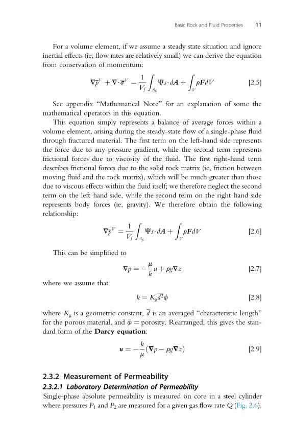
From first principles: with conservation of momentum we can consider avolume element (V) of fluid moving through porous material. V will have adifferent position at time t þ dt compared with that at time t, and it mayalso have a different volume (Fig. 2.5).
The rate of change in momentum with time (from t to t þ dt) equalsbody forces (gravity) þ stress (frictional forces).
V(t)V(t + δt)
Figure 2.5 Volume element of fluid.
10 Fundamentals of Applied Reservoir Engineering
For a volume element, if we assume a steady state situation and ignoreinertial effects (ie, flow rates are relatively small) we can derive the equationfrom conservation of momentum:
VpV þ V$sV ¼ 1Vf
ZAfs
Js$dAþZVrFdV [2.5]
See appendix “Mathematical Note” for an explanation of some themathematical operators in this equation.
This equation simply represents a balance of average forces within avolume element, arising during the steady-state flow of a single-phase fluidthrough fractured material. The first term on the left-hand side representsthe force due to any pressure gradient, while the second term representsfrictional forces due to viscosity of the fluid. The first right-hand termdescribes frictional forces due to the solid rock matrix (ie, friction betweenmoving fluid and the rock matrix), which will be much greater than thosedue to viscous effects within the fluid itself; we therefore neglect the secondterm on the left-hand side, while the second term on the right-hand siderepresents body forces (ie, gravity). We therefore obtain the followingrelationship:
VpV ¼ 1Vf
ZAfs
Js$dAþZVrFdV [2.6]
This can be simplified to
Vp ¼ �m
kuþ rgVz [2.7]
where we assume that
k ¼ Kgd2f [2.8]
where Kg is a geometric constant, d is an averaged “characteristic length”for the porous material, and f ¼ porosity. Rearranged, this gives the stan-dard form of the Darcy equation:
u ¼ � kmðVp� rgVzÞ [2.9]
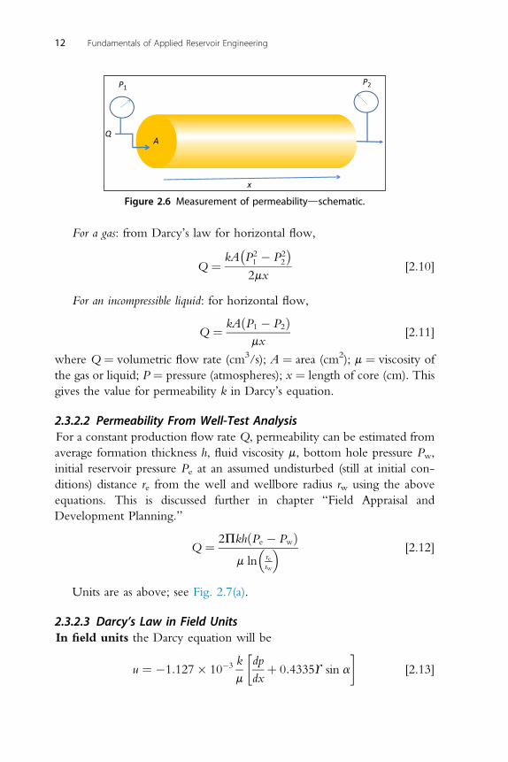
2.3.2 Measurement of Permeability2.3.2.1 Laboratory Determination of PermeabilitySingle-phase absolute permeability is measured on core in a steel cylinderwhere pressures P1 and P2 are measured for a given gas flow rateQ (Fig. 2.6).
Basic Rock and Fluid Properties 11
For a gas: from Darcy’s law for horizontal flow,
Q ¼ kA�P21 � P2
2
�2mx
[2.10]
For an incompressible liquid: for horizontal flow,
Q ¼ kAðP1 � P2Þmx
[2.11]
where Q ¼ volumetric flow rate (cm3/s); A ¼ area (cm2); m ¼ viscosity ofthe gas or liquid; P ¼ pressure (atmospheres); x ¼ length of core (cm). Thisgives the value for permeability k in Darcy’s equation.
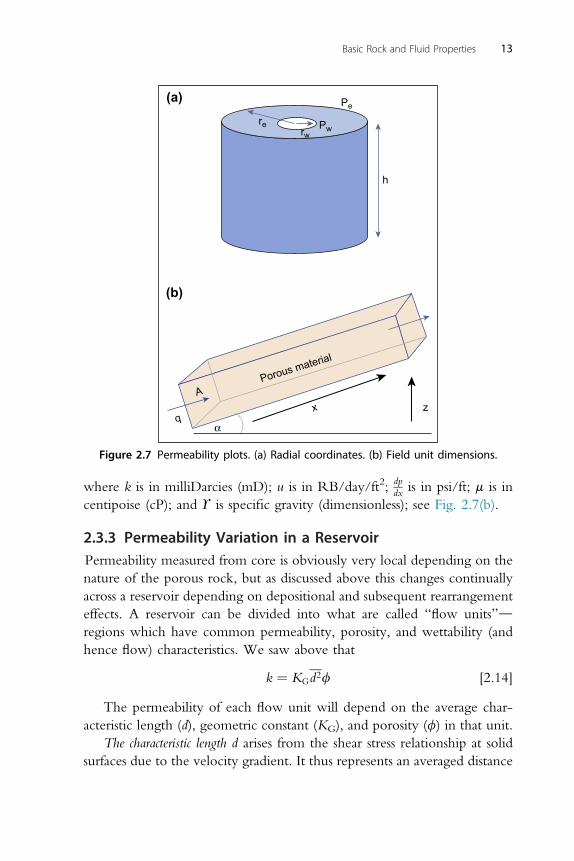
2.3.2.2 Permeability From Well-Test AnalysisFor a constant production flow rate Q, permeability can be estimated fromaverage formation thickness h, fluid viscosity m, bottom hole pressure Pw,initial reservoir pressure Pe at an assumed undisturbed (still at initial con-ditions) distance re from the well and wellbore radius rw using the aboveequations. This is discussed further in chapter “Field Appraisal andDevelopment Planning.”
Q ¼ 2PkhðPe � PwÞm ln
�rerw
� [2.12]
Units are as above; see Fig. 2.7(a).
2.3.2.3 Darcy’s Law in Field UnitsIn field units the Darcy equation will be
u ¼ �1:127� 10�3 km
�dpdx
þ 0:4335Y sin a
�[2.13]
A
P1P2
x
Q
Figure 2.6 Measurement of permeabilitydschematic.
12 Fundamentals of Applied Reservoir Engineering
where k is in milliDarcies (mD); u is in RB/day/ft2; dpdx is in psi/ft; m is in
centipoise (cP); and Y is specific gravity (dimensionless); see Fig. 2.7(b).
2.3.3 Permeability Variation in a ReservoirPermeability measured from core is obviously very local depending on thenature of the porous rock, but as discussed above this changes continuallyacross a reservoir depending on depositional and subsequent rearrangementeffects. A reservoir can be divided into what are called “flow units”dregions which have common permeability, porosity, and wettability (andhence flow) characteristics. We saw above that
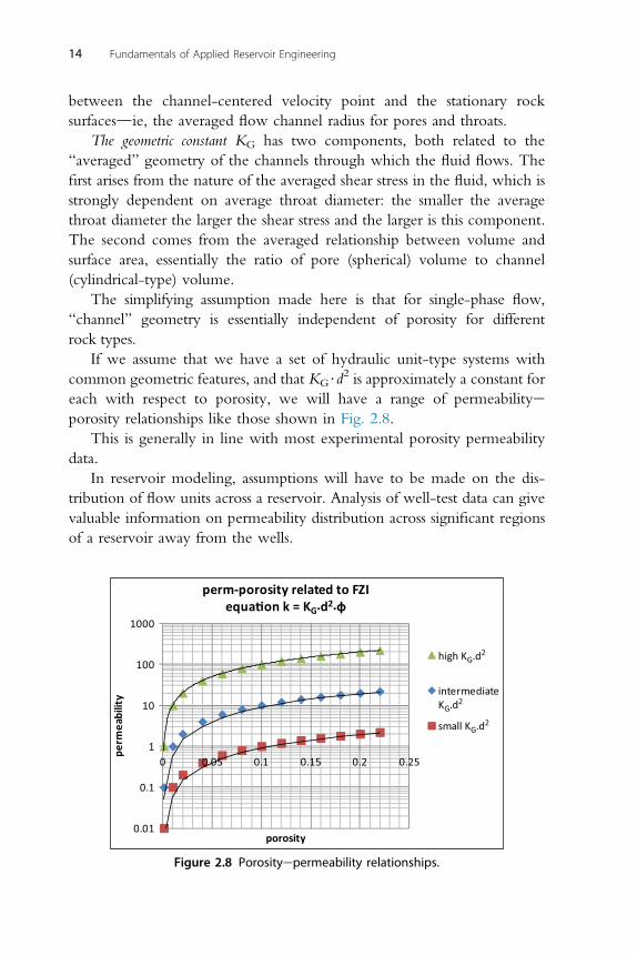
k ¼ KGd2f [2.14]
The permeability of each flow unit will depend on the average char-acteristic length (d), geometric constant (KG), and porosity (f) in that unit.
The characteristic length d arises from the shear stress relationship at solidsurfaces due to the velocity gradient. It thus represents an averaged distance
Pe
Pwre
rw
h
z
Porous material
Ax
qα
(a)
(b)
Figure 2.7 Permeability plots. (a) Radial coordinates. (b) Field unit dimensions.
Basic Rock and Fluid Properties 13
between the channel-centered velocity point and the stationary rocksurfacesdie, the averaged flow channel radius for pores and throats.
The geometric constant KG has two components, both related to the“averaged” geometry of the channels through which the fluid flows. Thefirst arises from the nature of the averaged shear stress in the fluid, which isstrongly dependent on average throat diameter: the smaller the averagethroat diameter the larger the shear stress and the larger is this component.The second comes from the averaged relationship between volume andsurface area, essentially the ratio of pore (spherical) volume to channel(cylindrical-type) volume.
The simplifying assumption made here is that for single-phase flow,“channel” geometry is essentially independent of porosity for differentrock types.
If we assume that we have a set of hydraulic unit-type systems withcommon geometric features, and that KG$d
2 is approximately a constant foreach with respect to porosity, we will have a range of permeabilityeporosity relationships like those shown in Fig. 2.8.
This is generally in line with most experimental porosity permeabilitydata.
In reservoir modeling, assumptions will have to be made on the dis-tribution of flow units across a reservoir. Analysis of well-test data can givevaluable information on permeability distribution across significant regionsof a reservoir away from the wells.
0.01
0.1
1
10
100
1000
0 0.05 0.1 0.15 0.2 0.25
perm
eabi
lity
porosity
perm-porosity related to FZIequa�on k = KG•d2•ф
high KG.d2
intermediateKG.d2
small KG.d2
Figure 2.8 Porosityepermeability relationships.
14 Fundamentals of Applied Reservoir Engineering
2.3.4 Vertical and Horizontal PermeabilityIt is normally (but not always) assumed that horizontal permeability is thesame in each direction; but vertical permeability is often, and particularly inclastics, significantly smaller than horizontal permeability when sedimentsare frequently poorly sorted, angular, and irregular. Vertical/horizontal(kv/kh) values are typically in the range 0.01e0.1.
2.4 WETTABILITY
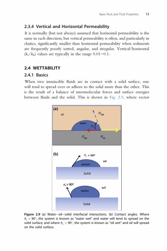
2.4.1 BasicsWhen two immiscible fluids are in contact with a solid surface, onewill tend to spread over or adhere to the solid more than the other. Thisis the result of a balance of intermolecular forces and surface energiesbetween fluids and the solid. This is shown in Fig. 2.9, where vector
Figure 2.9 (a) Watereoilesolid interfacial interactions. (b) Contact angles. Whereqc < 90� , the system is known as “water wet” and water will tend to spread on thesolid surface; and where qc > 90�, the system is known as “oil wet” and oil will spreadon the solid surface.
Basic Rock and Fluid Properties 15
forces are balanced at the oilewateresolid contact point, giving therelationship
sos � sws ¼ sow cos qc [2.15]
where sos ¼ the interfacial tension between oil and solid; sws ¼ the inter-facial tension between water and solid; sow ¼ the interfacial tension be-tween oil and water; and qc ¼ the contact angle between water and oilat the contact point measured through the water.
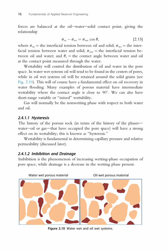
Wettability will control the distribution of oil and water in the porespace. In water wet systems oil will tend to be found in the centers of pores,while in oil wet systems oil will be retained around the solid grains (seeFig. 2.10). This will of course have a fundamental effect on oil recovery inwater flooding. Many examples of porous material have intermediatewettability where the contact angle is close to 90�. We can also haveshort-range variable or “mixed” wettability.
Gas will normally be the nonwetting phase with respect to both waterand oil.
2.4.1.1 HysteresisThe history of the porous rock (in terms of the history of the phasesdwatereoil or gasdthat have occupied the pore space) will have a strongeffect on its wettability; this is known as “hysteresis.”
Wettability is fundamental in determining capillary pressure and relativepermeability (discussed later).
2.4.1.2 Imbibition and DrainageImbibition is the phenomenon of increasing wetting-phase occupation ofpore space, while drainage is a decrease in the wetting phase present.
Water wet porous material Oil wet porous material
Figure 2.10 Water wet and oil wet systems.
16 Fundamentals of Applied Reservoir Engineering
2.4.2 Measuring WettabilitySeveral methods are available to measure a reservoir’s wetting preference.Core measurements include imbibition and centrifuge capillary pressuremeasurements (discussed below). An Amott imbibition test compares thespontaneous imbibition of oil and water to the total saturation changeobtained by flooding. We will also see later that capillary pressure andrelative permeability measurements give an idea of rock wettability.
2.5 SATURATION AND CAPILLARY PRESSURE
2.5.1 SaturationSaturation is the proportion of interconnected pore space occupied by agiven phase. For a gaseoilewater system,
Sw þ So þ Sg ¼ 1 [2.16]
where Sw ¼ water saturation, So ¼ oil saturation, and Sg ¼ gas saturation.
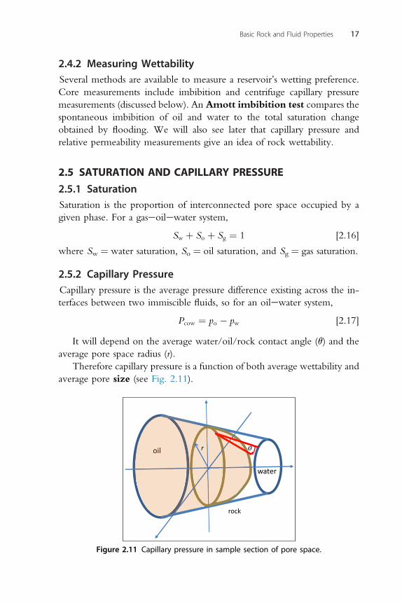
2.5.2 Capillary PressureCapillary pressure is the average pressure difference existing across the in-terfaces between two immiscible fluids, so for an oilewater system,
Pcow ¼ po � pw [2.17]
It will depend on the average water/oil/rock contact angle (q) and theaverage pore space radius (r).
Therefore capillary pressure is a function of both average wettability andaverage pore size (see Fig. 2.11).
rock
oil
water
oil ϴr
Figure 2.11 Capillary pressure in sample section of pore space.
Basic Rock and Fluid Properties 17
If we take an example section of pore space, it can be shown that thecapillary pressure between the wetting and nonwetting phases is given by
Pcnw ¼ 2$KGsnwcosðqÞ=rw [2.18]
where KG is a geometric constant dependent on the average geometry ofthe pore space, snw is the oil/water interfacial tension, and rw is the averageradius of wetting-phase-occupied pores.
This wetting-phase radius rw is a function of the saturation of thewetting phase. The smaller the wetting-phase saturation the more it will beconcentrated in smaller pores, so that rw will be small and hence thecapillary pressure will be larger. The smaller the interfacial tension betweenthe two phases the smaller will be the capillary pressure.
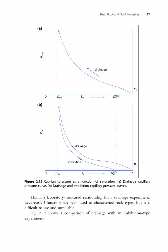
A drainage (decreasing wetting phase) capillary pressure curve is shownbelow (see Fig. 2.12(b)). Pb is the threshold pressuredthe minimum pressurerequired to initiate drainage displacement. Capillary pressure increases aswetting phase saturation decreases, since
Pcap ¼ 2KGs cosðqÞ=rw [2.19]
and it can be shown that
kf r24 ¼ K*Gr
2f
where K*G is another geological constant. Thus,
rfffiffiffiffiffiffiffiffik=f
p[2.20]
and
rwfr�SNw
�an[2.21]
so that,
Pcap ¼ K*Gs cos qffiffikf
q �SNw
�aw [2.22]
Leverett’s J function (a dimensionless capillary pressure) is defined as
JðSwÞ ¼ Pcap
s cos q
ffiffiffikf
s¼ K*
G�SNw
�aw [2.23]
where SNw ¼ Sw � Swc1� Swc � Sor
18 Fundamentals of Applied Reservoir Engineering
This is a laboratory-measured relationship for a drainage experiment.Leveretts’s J function has been used to characterize rock types, but it isdifficult to use and unreliable.
Fig. 2.12 shows a comparison of drainage with an imbibition-typeexperiment.
drainage
Pca
pP
cap
Swc Sw
drainage
imbibition
Pb
Pb
Swmax
Swmax
10
Swc Sw 10
(a)
(b)
Figure 2.12 Capillary pressure as a function of saturation. (a) Drainage capillarypressure curve. (b) Drainage and imbibition capillary pressure curves.
Basic Rock and Fluid Properties 19
Oil/water capillary pressure is of more significance than oil/gas capillarypressure, which is normally very small and can often be neglected.
2.5.3 Reservoir Saturation With DepthThe major importance of capillary pressure is its effect on the distribution ofphases in the reservoir with depth.
For each phase k, reservoir pressure increases with depth (z) dependingon phase density:
dPk
dz¼ rk g [2.24]
and since,
Po � Pw ¼ Pcow
dPcow
dz¼ �ðro � rwÞ$g [2.25]
so
DPcow
Dz¼ �ðro � rwÞ$g [2.26]
if Dz ¼ width of transition zone, where
DPcow ¼ PcowðSo ¼ 1� SwcÞ � PcowðSo ¼ 0Þbut
PcowðSo ¼ 0Þ ¼ 0
so that
Dz ¼ �PcowðSo ¼ 1� SwcÞðro � rwÞ$g
[2.27]
High permeability or contact angle (close to 90�) results in smallcapillary pressures, thus in this case we have a smaller transition zone. Lowpermeability or small contact angle systems (with large capillary pressures)will have wide transition zones.
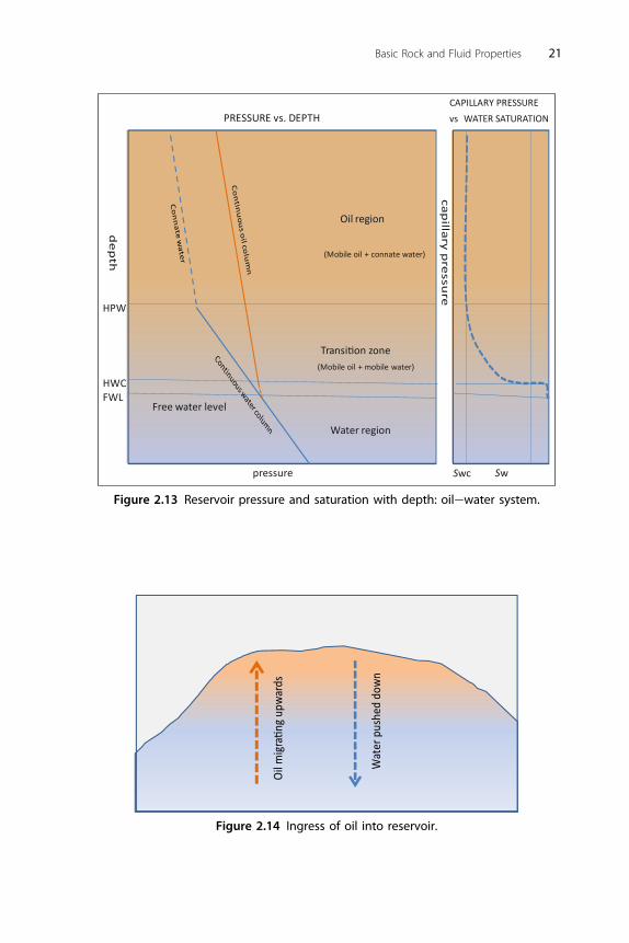
Fig. 2.13 shows a schematic for an oilewater reservoir of oil and waterpressures as a function of depth (left-hand plot) and of oil/water capillarypressure as a function of water saturation (right-hand plot).
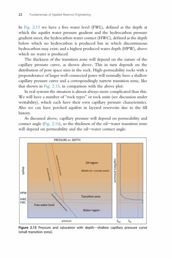
Geologically, the reservoir will have initially been filled with water(Sw ¼ 100%). Oil migrating up from below (oil having a lower density thanwater) will have gradually displaced waterda drainage process (see Fig. 2.14).
20 Fundamentals of Applied Reservoir Engineering
(Mobile oil + connate water)
Free water levelFWL
Transi on zone
de
pth
pressure
(Mobile oil + mobile water)
Oil region
Water region
capillary
pre
ssure
SwSwc
PRESSURE vs. DEPTHCAPILLARY PRESSUREvs WATER SATURATION
HPW
HWC
Figure 2.13 Reservoir pressure and saturation with depth: oilewater system.
Oil m
igra
�ng
upw
ards
Wat
er p
ushe
d do
wn
Figure 2.14 Ingress of oil into reservoir.
Basic Rock and Fluid Properties 21
In Fig. 2.13 we have a free water level (FWL), defined as the depth atwhich the aquifer water pressure gradient and the hydrocarbon pressuregradient meet; the hydrocarbon water contact (HWC), defined as the depthbelow which no hydrocarbon is produced but in which discontinuoushydrocarbon may exist; and a highest produced water depth (HPW), abovewhich no water is produced.
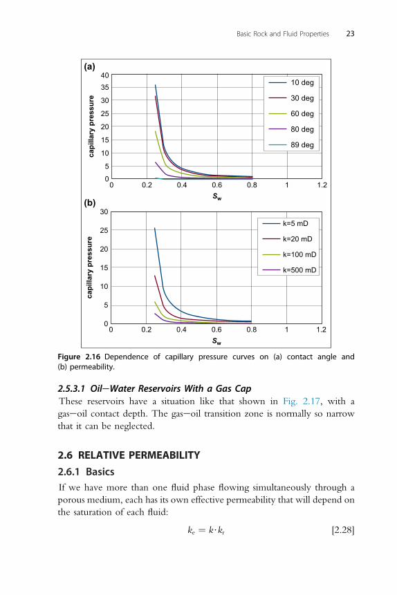
The thickness of the transition zone will depend on the nature of thecapillary pressure curve, as shown above. This in turn depends on thedistribution of pore space sizes in the rock. High-permeability rocks with apreponderance of larger well-connected pores will normally have a shallowcapillary pressure curve and a correspondingly narrow transition zone, likethat shown in Fig. 2.15, in comparison with the above plot.
In real systems the situation is almost always more complicated than this.We will have a number of “rock types” or rock units (see discussion underwettability), which each have their own capillary pressure characteristics.Also we can have perched aquifers in layered reservoirs due to the fillhistory.
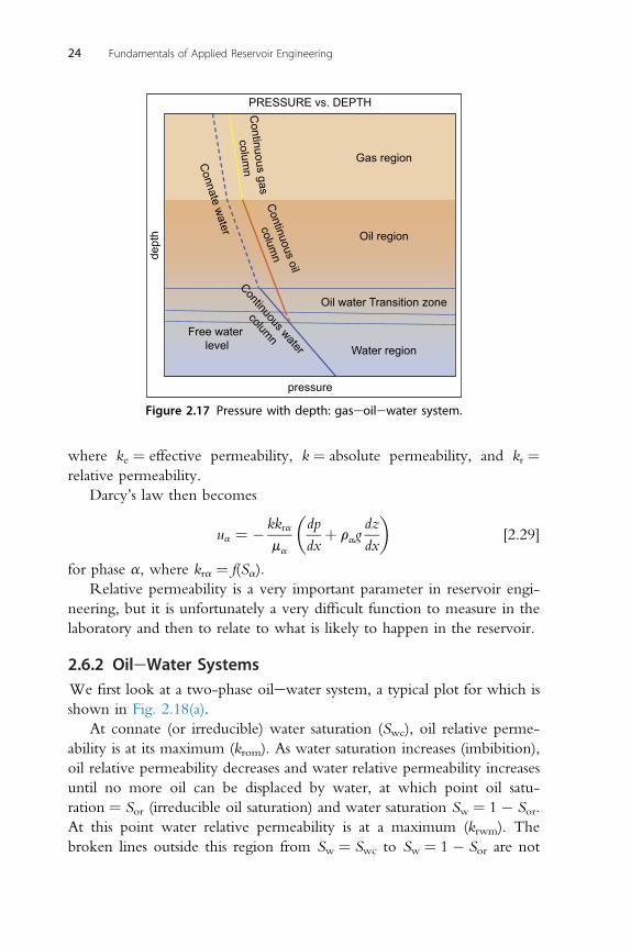
As discussed above, capillary pressure will depend on permeability andcontact angle (Fig. 2.16), so the thickness of the oilewater transition zonewill depend on permeability and the oilewater contact angle.
(Mobile oil + connate water)
Free water levelFWL
Transi�on zone
depth
pressure
Oil region
Water region
capillarypressure
SwSwc
PRESSURE vs. DEPTH
HPW
HWC
Figure 2.15 Pressure and saturation with depthdshallow capillary pressure curve(small transition zone).
22 Fundamentals of Applied Reservoir Engineering
2.5.3.1 OileWater Reservoirs With a Gas CapThese reservoirs have a situation like that shown in Fig. 2.17, with agaseoil contact depth. The gaseoil transition zone is normally so narrowthat it can be neglected.
2.6 RELATIVE PERMEABILITY
2.6.1 BasicsIf we have more than one fluid phase flowing simultaneously through aporous medium, each has its own effective permeability that will depend onthe saturation of each fluid:
ke ¼ k$kr [2.28]
40
capi
llary
pre
ssur
e35
30
25
20
15
10
5
00 0.2 0.4 0.6
Sw
(a)
0.8 1 1.2
10 deg
30 deg
60 deg
80 deg
89 deg
30
capi
llary
pre
ssur
e
25
20
15
10
5
00 0.2 0.4 0.6
Sw
(b)
0.8 1 1.2
k=5 mD
k=20 mD
k=100 mD
k=500 mD
Figure 2.16 Dependence of capillary pressure curves on (a) contact angle and(b) permeability.
Basic Rock and Fluid Properties 23
where ke ¼ effective permeability, k ¼ absolute permeability, and kr ¼relative permeability.
Darcy’s law then becomes
ua ¼ � kkrama
dpdx
þ ragdzdx
[2.29]
for phase a, where kra ¼ f(Sa).Relative permeability is a very important parameter in reservoir engi-
neering, but it is unfortunately a very difficult function to measure in thelaboratory and then to relate to what is likely to happen in the reservoir.
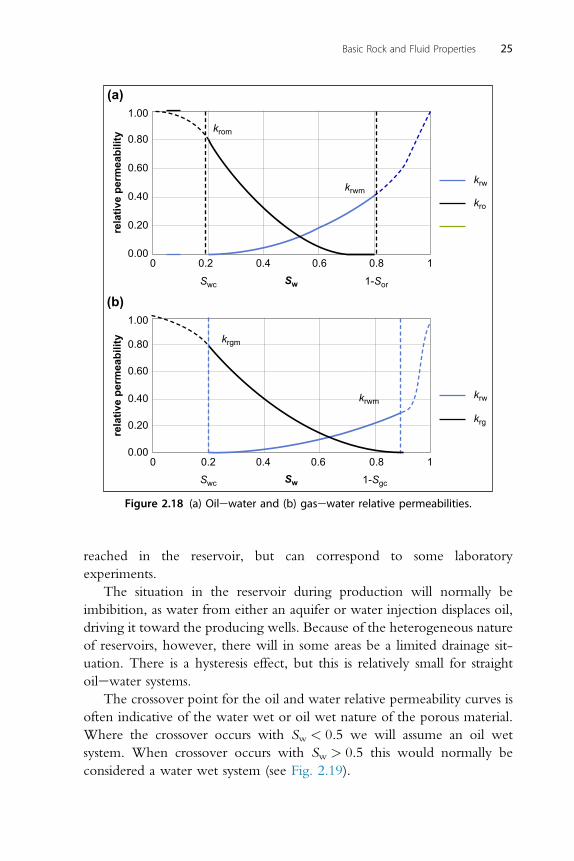
2.6.2 OileWater SystemsWe first look at a two-phase oilewater system, a typical plot for which isshown in Fig. 2.18(a).
At connate (or irreducible) water saturation (Swc), oil relative perme-ability is at its maximum (krom). As water saturation increases (imbibition),oil relative permeability decreases and water relative permeability increasesuntil no more oil can be displaced by water, at which point oil satu-ration ¼ Sor (irreducible oil saturation) and water saturation Sw ¼ 1 � Sor.At this point water relative permeability is at a maximum (krwm). Thebroken lines outside this region from Sw ¼ Swc to Sw ¼ 1 � Sor are not
PRESSURE vs. DEPTH
Gas region
Continuous gas
columnConnate w
aterContinuous water
columnC
ontinuous oil
column
Oil region
Water regionFree water
level
pressure
dept
h
Oil water Transition zone
Figure 2.17 Pressure with depth: gaseoilewater system.
24 Fundamentals of Applied Reservoir Engineering
reached in the reservoir, but can correspond to some laboratoryexperiments.
The situation in the reservoir during production will normally beimbibition, as water from either an aquifer or water injection displaces oil,driving it toward the producing wells. Because of the heterogeneous natureof reservoirs, however, there will in some areas be a limited drainage sit-uation. There is a hysteresis effect, but this is relatively small for straightoilewater systems.
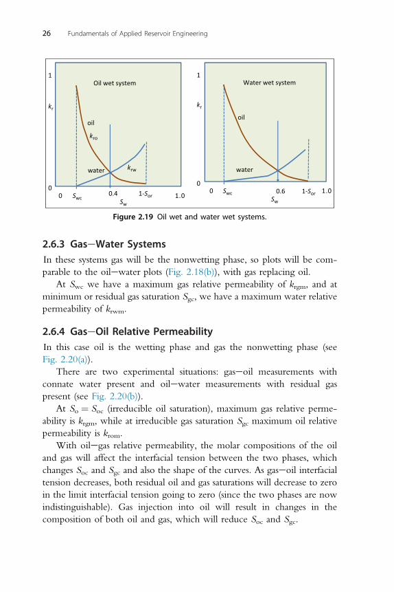
The crossover point for the oil and water relative permeability curves isoften indicative of the water wet or oil wet nature of the porous material.Where the crossover occurs with Sw < 0.5 we will assume an oil wetsystem. When crossover occurs with Sw > 0.5 this would normally beconsidered a water wet system (see Fig. 2.19).
1.00
(a)re
lativ
e pe
rmea
bilit
y 0.80
0.60
0.40
0.20
0.000 0.2
Swc
krom
kro
krwkrwm
Sw 1-Sor
0.4 0.6 0.8 1
1.00
(b)
rela
tive
perm
eabi
lity
0.80
0.60
0.40
0.20
0.000 0.2
Swc
krg
krw
Sw 1-Sgc
0.4 0.6 0.8 1
krgm
krwm
Figure 2.18 (a) Oilewater and (b) gasewater relative permeabilities.
Basic Rock and Fluid Properties 25
2.6.3 GaseWater SystemsIn these systems gas will be the nonwetting phase, so plots will be com-parable to the oilewater plots (Fig. 2.18(b)), with gas replacing oil.
At Swc we have a maximum gas relative permeability of krgm, and atminimum or residual gas saturation Sgc, we have a maximum water relativepermeability of krwm.
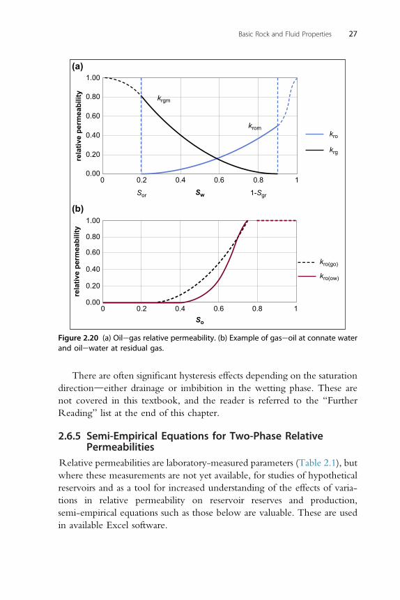
2.6.4 GaseOil Relative PermeabilityIn this case oil is the wetting phase and gas the nonwetting phase (seeFig. 2.20(a)).
There are two experimental situations: gaseoil measurements withconnate water present and oilewater measurements with residual gaspresent (see Fig. 2.20(b)).
At So ¼ Soc (irreducible oil saturation), maximum gas relative perme-ability is krgm, while at irreducible gas saturation Sgc maximum oil relativepermeability is krom.
With oilegas relative permeability, the molar compositions of the oiland gas will affect the interfacial tension between the two phases, whichchanges Soc and Sgc and also the shape of the curves. As gaseoil interfacialtension decreases, both residual oil and gas saturations will decrease to zeroin the limit interfacial tension going to zero (since the two phases are nowindistinguishable). Gas injection into oil will result in changes in thecomposition of both oil and gas, which will reduce Soc and Sgc.
0.10Sw
Swc
oil
water
kr kr
0
1
1-Sor
Oil wet system
0.4 0.10Sw
Swc
oil
water
0
1
1-Sor
Water wet system
0.6
kro
krw
Figure 2.19 Oil wet and water wet systems.
26 Fundamentals of Applied Reservoir Engineering
There are often significant hysteresis effects depending on the saturationdirectiondeither drainage or imbibition in the wetting phase. These arenot covered in this textbook, and the reader is referred to the “FurtherReading” list at the end of this chapter.
2.6.5 Semi-Empirical Equations for Two-Phase RelativePermeabilities
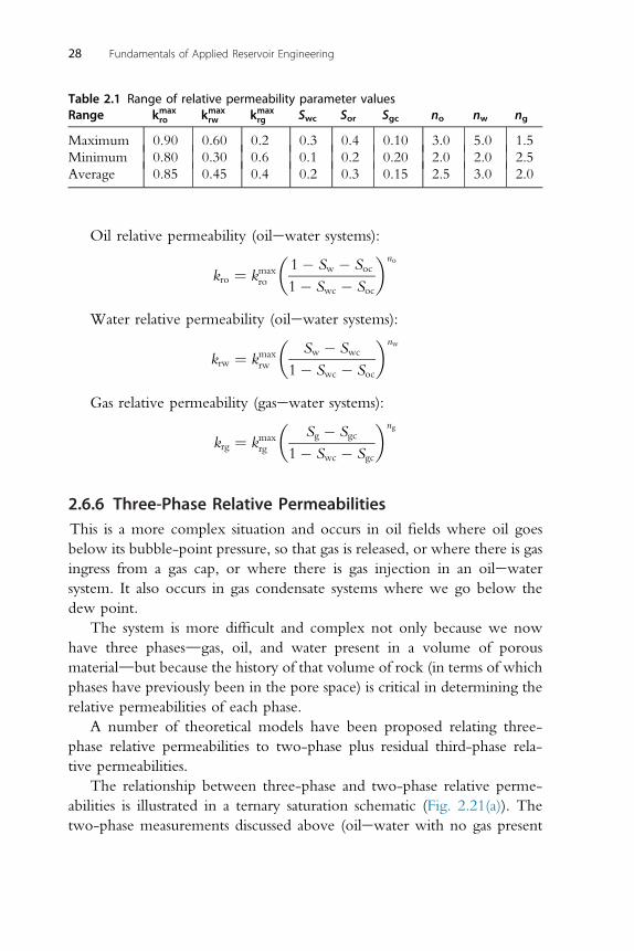
Relative permeabilities are laboratory-measured parameters (Table 2.1), butwhere these measurements are not yet available, for studies of hypotheticalreservoirs and as a tool for increased understanding of the effects of varia-tions in relative permeability on reservoir reserves and production,semi-empirical equations such as those below are valuable. These are usedin available Excel software.
krgm
krom
1.00(a)
rela
tive
perm
eabi
lity 0.80
0.60
0.40
0.20
0.000 0.2
Sor
kro
krg
Sw 1-Sgr
0.4 0.6 0.8 1
1.00(b)
rela
tive
perm
eabi
lity
0.80
0.60
0.40
0.20
0.000 0.2
So
kro(go)
kro(ow)
0.4 0.6 0.8 1
Figure 2.20 (a) Oilegas relative permeability. (b) Example of gaseoil at connate waterand oilewater at residual gas.
Basic Rock and Fluid Properties 27
Oil relative permeability (oilewater systems):
kro ¼ kmaxro
1� Sw � Soc1� Swc � Soc
no
Water relative permeability (oilewater systems):
krw ¼ kmaxrw
Sw � Swc
1� Swc � Soc
nw
Gas relative permeability (gasewater systems):
krg ¼ kmaxrg
Sg � Sgc
1� Swc � Sgc
ng
2.6.6 Three-Phase Relative PermeabilitiesThis is a more complex situation and occurs in oil fields where oil goesbelow its bubble-point pressure, so that gas is released, or where there is gasingress from a gas cap, or where there is gas injection in an oilewatersystem. It also occurs in gas condensate systems where we go below thedew point.
The system is more difficult and complex not only because we nowhave three phasesdgas, oil, and water present in a volume of porousmaterialdbut because the history of that volume of rock (in terms of whichphases have previously been in the pore space) is critical in determining therelative permeabilities of each phase.
A number of theoretical models have been proposed relating three-phase relative permeabilities to two-phase plus residual third-phase rela-tive permeabilities.
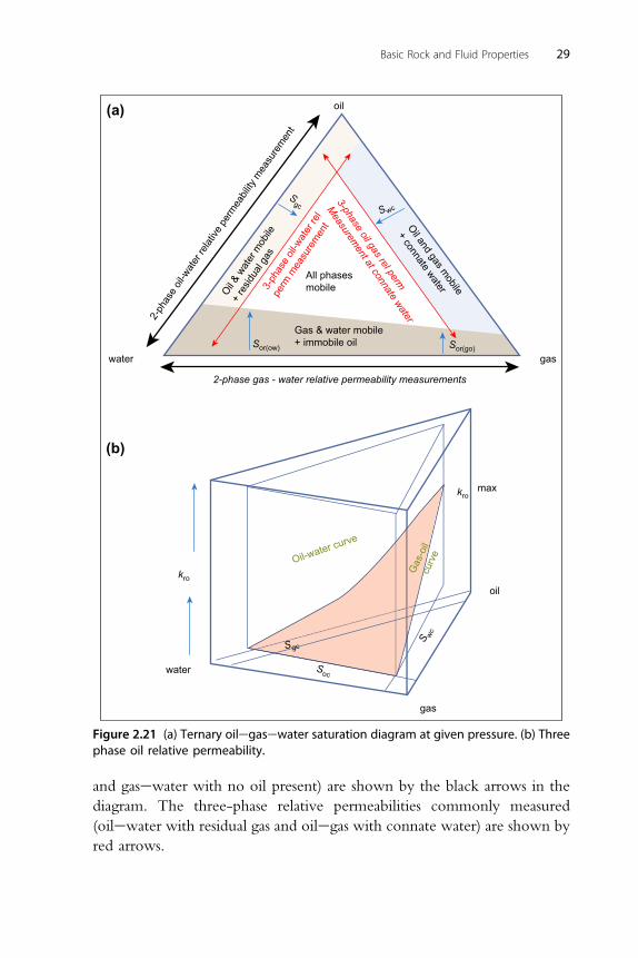
The relationship between three-phase and two-phase relative perme-abilities is illustrated in a ternary saturation schematic (Fig. 2.21(a)). Thetwo-phase measurements discussed above (oilewater with no gas present
Table 2.1 Range of relative permeability parameter valuesRange kmax
and gasewater with no oil present) are shown by the black arrows in thediagram. The three-phase relative permeabilities commonly measured(oilewater with residual gas and oilegas with connate water) are shown byred arrows.
oil
Sgc
S wc
All phasesmobile
2-phase gas - water relative permeability measurements
Sor(ow) Sor(go)gas
Gas & water mobile + immobile oil
water
(a)
(b)
kro
kromax
oil
water
gas
Soc
S wc
Sgc
Oil-water curve
Gas
-oil
curv
e
Oil & w
ater
mob
ile
+ re
sidua
l gas
3-ph
ase
oil-w
ater
rel
perm
mea
sure
men
t
3-phase oil gas rel perm
Measurem
ent at connate waterOil and gas m
obile
+ connate water
2-ph
ase
oil-w
ater
relat
ive p
erm
eabil
ity m
easu
rem
ent
Figure 2.21 (a) Ternary oilegasewater saturation diagram at given pressure. (b) Threephase oil relative permeability.
Basic Rock and Fluid Properties 29
So, for example, oil-phase relative permeability in a three-phase systemcan be represented as shown in Fig. 2.21(b).
There are a number of relationships that interpolate the relativepermeability of oil into a three-mobile-phase region from two-phaseoilewater þ residual gas and gaseoil þ connate water systems (redarrowsdgray in print versions in Fig. 2.21). An example of this is
kro ¼ SNo kroðSo; SwcÞ$kroðSgc; SoÞkmaxro $
�1� SN
g
��1� SN
w
� [2.30]
where SNo ; SNg ; and SNw are normalized oil, gas, and water saturations.
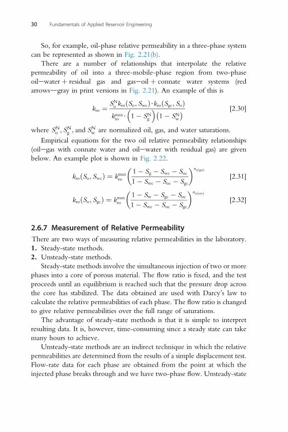
Empirical equations for the two oil relative permeability relationships(oilegas with connate water and oilewater with residual gas) are givenbelow. An example plot is shown in Fig. 2.22.
kroðSo; SwcÞ ¼ kmaxro
1� Sg � Swc � Soc1� Swc � Soc � Sgc
noðgoÞ[2.31]
kroðSo; SgcÞ ¼ kmaxro
1� Sw � Sgc � Soc1� Swc � Soc � Sgc
noðowÞ[2.32]
2.6.7 Measurement of Relative PermeabilityThere are two ways of measuring relative permeabilities in the laboratory.1. Steady-state methods.2. Unsteady-state methods.
Steady-state methods involve the simultaneous injection of two or morephases into a core of porous material. The flow ratio is fixed, and the testproceeds until an equilibrium is reached such that the pressure drop acrossthe core has stabilized. The data obtained are used with Darcy’s law tocalculate the relative permeabilities of each phase. The flow ratio is changedto give relative permeabilities over the full range of saturations.
The advantage of steady-state methods is that it is simple to interpretresulting data. It is, however, time-consuming since a steady state can takemany hours to achieve.
Unsteady-state methods are an indirect technique in which the relativepermeabilities are determined from the results of a simple displacement test.Flow-rate data for each phase are obtained from the point at which theinjected phase breaks through and we have two-phase flow. Unsteady-state
30 Fundamentals of Applied Reservoir Engineering
methods have the advantage of being quick to carry out, but data are muchmore difficult to interpret.
2.6.8 Excel Software for Producing Empirical RelativePermeability and Capillary Pressure Curves
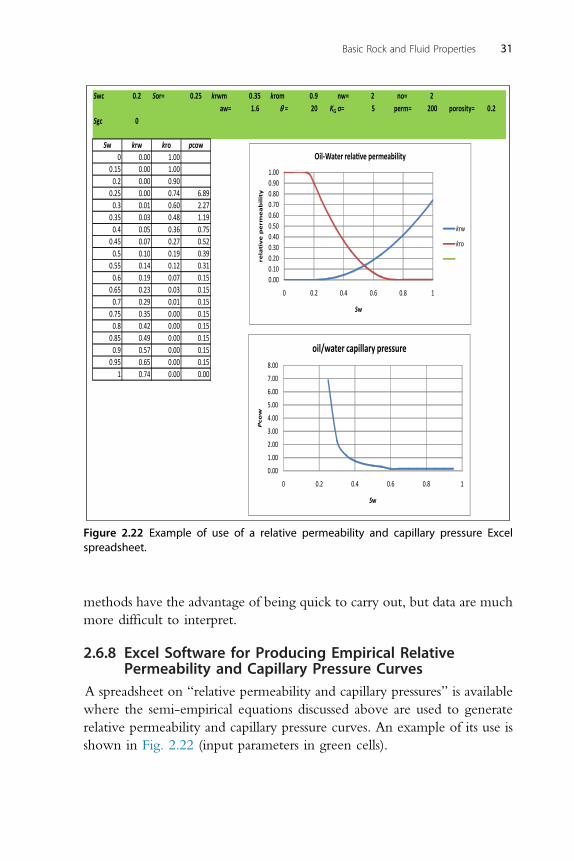
A spreadsheet on “relative permeability and capillary pressures” is availablewhere the semi-empirical equations discussed above are used to generaterelative permeability and capillary pressure curves. An example of its use isshown in Fig. 2.22 (input parameters in green cells).
Figure 2.22 Example of use of a relative permeability and capillary pressure Excelspreadsheet.
Basic Rock and Fluid Properties 31
The effect of the various input parameters on two-phase oilewater andgasewater curves and on oilewater with residual gas and oilegas withconnate water can be examined.
2.7 RESERVOIR FLUIDS
2.7.1 BasicsReservoir fluids are a complex mixture of many hundreds of hydrocarboncomponents plus a number of nonhydrocarbons (referred to as inerts).
We will be considering• phase behavior of hydrocarbon mixtures;• dynamics of reservoir behavior and production methods as a function of
fluid typedvolumetrics; and• laboratory investigation of reservoir fluids.
Reservoirs contain a mixture of hydrocarbons and inerts.Hydrocarbons will be C1 to Cn where n > 200.The main inerts are carbon dioxide (CO2), nitrogen (N2), and hydrogen
sulphide (H2S).Hydrocarbons are generated in “source rock” by the breakdown of
organic material at high temperature and pressure, then migrate upwardsinto “traps” where permeable rock above displaces the water originallypresent (see Fig. 2.23).
The fluid properties of any particular mixture will depend on reservoirtemperature and pressure.
The nature of the hydrocarbon mixture generated will depend on theoriginal biological material present, the temperature of the source rock andthe pressure, temperature, and time taken.
A number of phases of migration can occur, with different inputsmixing in the reservoir trap. In the reservoir we can eventually havesingle-phase (unsaturated) or two-phase (saturated) systems.
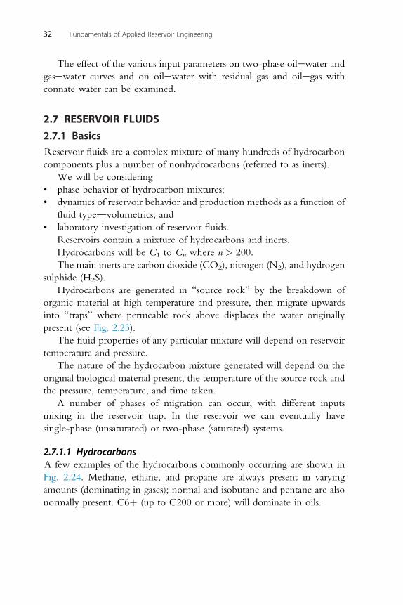
2.7.1.1 HydrocarbonsA few examples of the hydrocarbons commonly occurring are shown inFig. 2.24. Methane, ethane, and propane are always present in varyingamounts (dominating in gases); normal and isobutane and pentane are alsonormally present. C6þ (up to C200 or more) will dominate in oils.
32 Fundamentals of Applied Reservoir Engineering
Figure 2.23 Migration and accumulation of hydrocarbons in a reservoir.
Figure 2.24 Some common reservoir hydrocarbons.
Basic Rock and Fluid Properties 33
2.7.1.2 InertsCarbon dioxide and hydrogen sulphide are a problem for the petroleumengineerdthey give acid solutions in water which are corrosive to metalpipelines and wellbore pipes. We also have the cost of removal, and in someH2S cases even the disposal of unwanted sulfur is a problem.
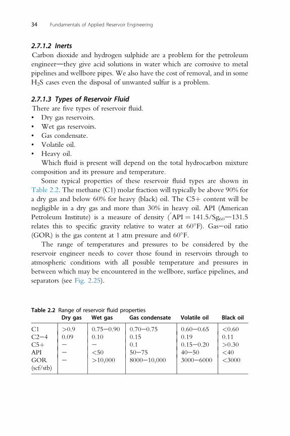
2.7.1.3 Types of Reservoir FluidThere are five types of reservoir fluid.• Dry gas reservoirs.• Wet gas reservoirs.• Gas condensate.• Volatile oil.• Heavy oil.
Which fluid is present will depend on the total hydrocarbon mixturecomposition and its pressure and temperature.
Some typical properties of these reservoir fluid types are shown inTable 2.2. The methane (C1) molar fraction will typically be above 90% fora dry gas and below 60% for heavy (black) oil. The C5þ content will benegligible in a dry gas and more than 30% in heavy oil. API (AmericanPetroleum Institute) is a measure of density (
�API ¼ 141.5/Sg60d131.5
relates this to specific gravity relative to water at 60�F). Gaseoil ratio(GOR) is the gas content at 1 atm pressure and 60�F.
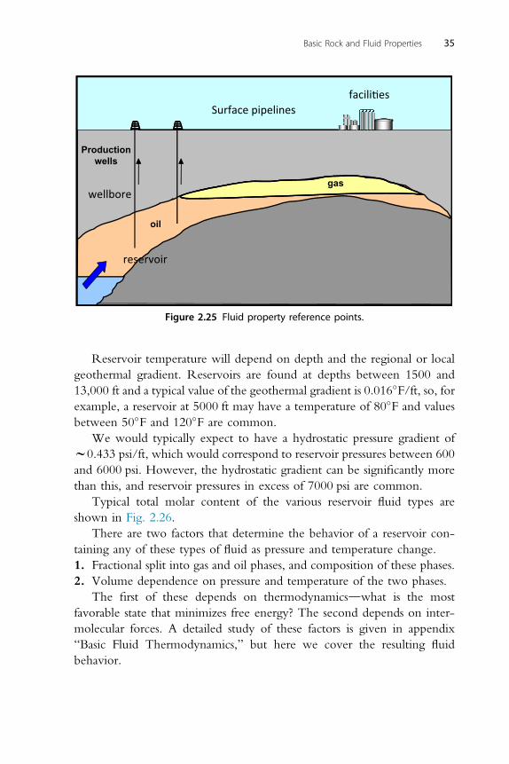
The range of temperatures and pressures to be considered by thereservoir engineer needs to cover those found in reservoirs through toatmospheric conditions with all possible temperature and pressures inbetween which may be encountered in the wellbore, surface pipelines, andseparators (see Fig. 2.25).
Table 2.2 Range of reservoir fluid propertiesDry gas Wet gas Gas condensate Volatile oil Black oil
C1 >0.9 0.75e0.90 0.70e0.75 0.60e0.65 <0.60C2e4 0.09 0.10 0.15 0.19 0.11C5þ e e 0.1 0.15e0.20 >0.30API e <50 50e75 40e50 <40GOR(scf/stb)
e >10,000 8000e10,000 3000e6000 <3000
34 Fundamentals of Applied Reservoir Engineering
Reservoir temperature will depend on depth and the regional or localgeothermal gradient. Reservoirs are found at depths between 1500 and13,000 ft and a typical value of the geothermal gradient is 0.016�F/ft, so, forexample, a reservoir at 5000 ft may have a temperature of 80�F and valuesbetween 50�F and 120�F are common.
We would typically expect to have a hydrostatic pressure gradient ofw0.433 psi/ft, which would correspond to reservoir pressures between 600and 6000 psi. However, the hydrostatic gradient can be significantly morethan this, and reservoir pressures in excess of 7000 psi are common.
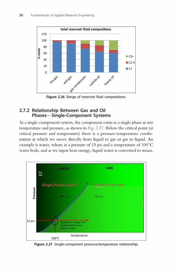
Typical total molar content of the various reservoir fluid types areshown in Fig. 2.26.
There are two factors that determine the behavior of a reservoir con-taining any of these types of fluid as pressure and temperature change.1. Fractional split into gas and oil phases, and composition of these phases.2. Volume dependence on pressure and temperature of the two phases.
The first of these depends on thermodynamicsdwhat is the mostfavorable state that minimizes free energy? The second depends on inter-molecular forces. A detailed study of these factors is given in appendix“Basic Fluid Thermodynamics,” but here we cover the resulting fluidbehavior.
gas
oil
Productionwells
facili�esSurface pipelines
wellbore
reservoir
Figure 2.25 Fluid property reference points.
Basic Rock and Fluid Properties 35
2.7.2 Relationship Between Gas and OilPhasesdSingle-Component Systems
In a single-component system, the component exists as a single phase at anytemperature and pressure, as shown in Fig. 2.27. Below the critical point (atcritical pressure and temperature) there is a pressure-temperature combi-nation at which we move directly from liquid to gas or gas to liquid. Anexample is water, where at a pressure of 15 psi and a temperature of 100�Cwater boils, and as we input heat energy, liquid water is converted to steam.
0
20
40
60
80
100
120%
mol
ar
total reservoir fluid composi�ons
C5+
C2-4
C1
Figure 2.26 Range of reservoir fluid compositions.
Pres
sure
DryGas
c
LIQUID GAS
temperature
Single Phase GasSingle Phase Liquid
100% liquid
Single Phase Gas
100% gas
15 psi
100°C
Liquid boils –energy (heatof vaporisa on) in put –volume change
The temperature will remain constant at 100�C until all the water is in thegaseous phase.
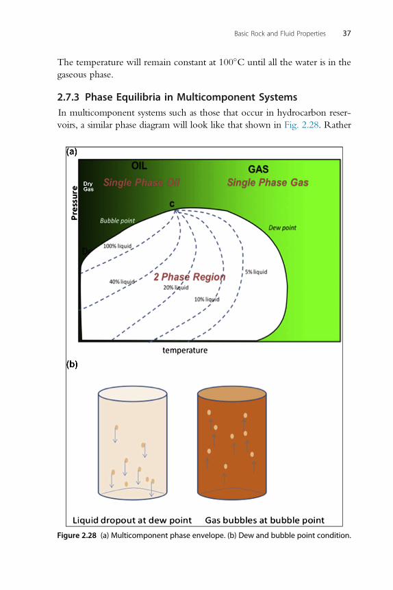
2.7.3 Phase Equilibria in Multicomponent SystemsIn multicomponent systems such as those that occur in hydrocarbon reser-voirs, a similar phase diagram will look like that shown in Fig. 2.28. Rather
Figure 2.28 (a) Multicomponent phase envelope. (b) Dew and bubble point condition.
Basic Rock and Fluid Properties 37
than a line division between gas and liquid, we now have a two-phase regionwhere various proportions of the gas and oil phases coexist.
This represents the pressure/temperature (PT) two-phase envelope for aparticular hydrocarbon mixture. At the temperatures and pressures in thegreen areas we have single-phase systems with this mixture. To the right ofthe critical point (C) we have a gas, so that if we drop the pressure until wecross the dew-point line a liquid drops out; and to the left an oil, wheredropping the pressure to bubble-point pressure bubbles of gas appear.However, in the white area this mixture cannot exist as a single phase andwill spontaneously split into a two-phase gas and oil system (see appendix:Mathematical Note). The percentage of liquid is shown by the broken linesinside this two-phase region. We can see that if temperature is kept constantand the pressure is reduced, the percentage of liquid increases beforeeventually decreasing again.
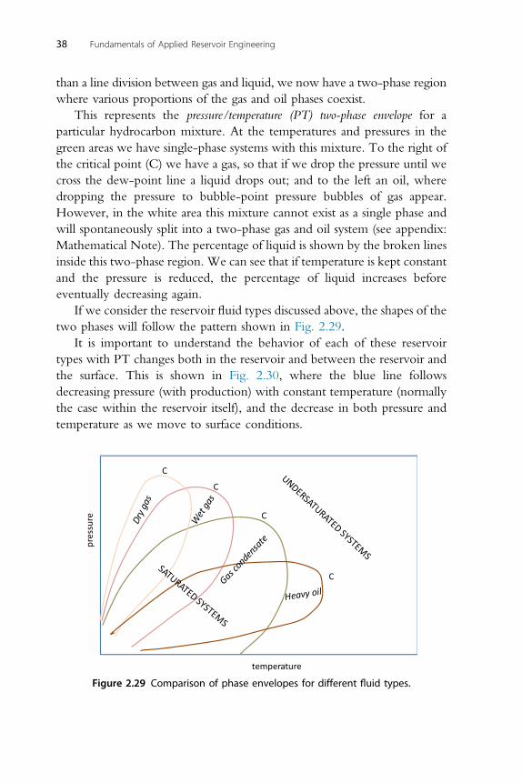
If we consider the reservoir fluid types discussed above, the shapes of thetwo phases will follow the pattern shown in Fig. 2.29.
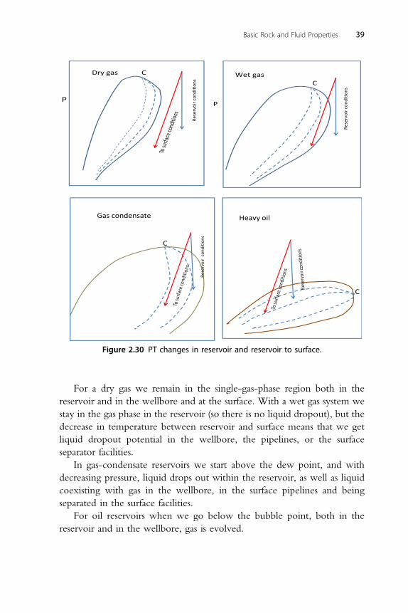
It is important to understand the behavior of each of these reservoirtypes with PT changes both in the reservoir and between the reservoir andthe surface. This is shown in Fig. 2.30, where the blue line followsdecreasing pressure (with production) with constant temperature (normallythe case within the reservoir itself), and the decrease in both pressure andtemperature as we move to surface conditions.
C
C
C
C
pres
sure
temperature
Figure 2.29 Comparison of phase envelopes for different fluid types.
38 Fundamentals of Applied Reservoir Engineering
For a dry gas we remain in the single-gas-phase region both in thereservoir and in the wellbore and at the surface. With a wet gas system westay in the gas phase in the reservoir (so there is no liquid dropout), but thedecrease in temperature between reservoir and surface means that we getliquid dropout potential in the wellbore, the pipelines, or the surfaceseparator facilities.
In gas-condensate reservoirs we start above the dew point, and withdecreasing pressure, liquid drops out within the reservoir, as well as liquidcoexisting with gas in the wellbore, in the surface pipelines and beingseparated in the surface facilities.
For oil reservoirs when we go below the bubble point, both in thereservoir and in the wellbore, gas is evolved.
CC
Dry gas
Rese
rvoi
r con
dion
s
P P
Wet gas
Rese
rvoi
r con
dion
s
C
Gas condensate
Rese
rvoi
r co
ndi
ons
C
Heavy oil
Figure 2.30 PT changes in reservoir and reservoir to surface.
Basic Rock and Fluid Properties 39
2.7.3.1 A Different RepresentationdTwo-PseudocomponentPressure Composition Plots
The above PT plots are standard representation for pressure/volume/temperature (PVT) properties, but are often misleadingdparticularly forthe reservoir. In this case temperature is normally more or less constantanyway. It must be remembered that the above PT plots are for a fixedhydrocarbon mixture composition.
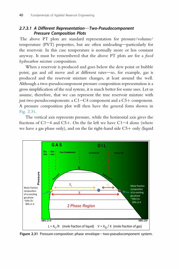
When a reservoir is produced and goes below the dew point or bubblepoint, gas and oil move and at different ratesdso, for example, gas isproduced and the reservoir mixture changes, at least around the well.Although a two-pseudocomponent pressure composition representation is agross simplification of the real system, it is much better for some uses. Let usassume, therefore, that we can represent the true reservoir mixture withjust two pseudocomponents: a C1eC4 component and a C5þ component.A pressure composition plot will then have the general form shown inFig. 2.31.
The vertical axis represents pressure, while the horizontal axis gives thefractions of C1e4 and C5þ. On the far left we have C1e4 alone (wherewe have a gas phase only), and on the far right-hand side C5þ only (liquid
Pre
ssur
e
DryGas
WetGas
Gas Condensate Volatile Oil Heavy Oil
c
100% C1-4 100% C5+
G A S O I L
2 Phase Region
L = XL /X (mole frac�on of liquid) V = XG / X (mole frac�on of gas)
at all pressures). The areas in green represent a single-phase regiondgas tothe left of the critical point and liquid to the right. In the white regioncompositions cannot exist as single phases at these pressures, but split into agas and a liquid whose compositions correspond to the points at the ends ofthe tie lines (dotted lines in the figure).
In this example, at the pressure shown the gas will have a mole fractionof w90% C1e4 and 10% C5þ. The coexisting liquid phase has 70% C5þand 30% C1e4. The number of moles of each phase is given by thefractions L ¼ XL/X and V ¼ XV/X. The green two-phase region is splitinto regions where decreasing pressure gives dry gas, wet gas, gascondensate, volatile and heavy oil.
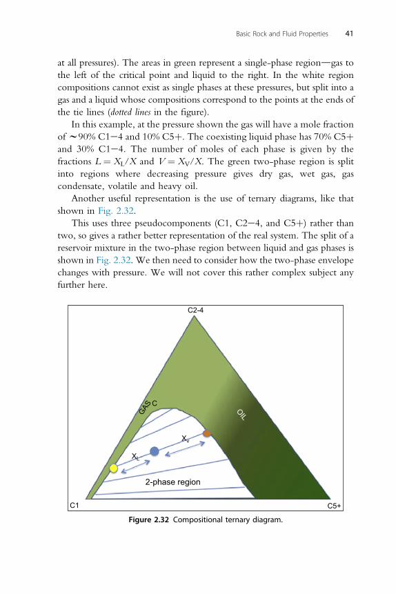
Another useful representation is the use of ternary diagrams, like thatshown in Fig. 2.32.
This uses three pseudocomponents (C1, C2e4, and C5þ) rather thantwo, so gives a rather better representation of the real system. The split of areservoir mixture in the two-phase region between liquid and gas phases isshown in Fig. 2.32. We then need to consider how the two-phase envelopechanges with pressure. We will not cover this rather complex subject anyfurther here.
C2-4
GASC
OIL
Xv
XL
2-phase region
C1 C5+
Figure 2.32 Compositional ternary diagram.
Basic Rock and Fluid Properties 41
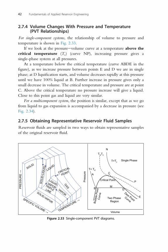
2.7.4 Volume Changes With Pressure and Temperature(PVT Relationships)
For single-component systems, the relationship of volume to pressure andtemperature is shown in Fig. 2.33.
If we look at the pressureevolume curve at a temperature above thecritical temperature (Tc) (curve NP), increasing pressure gives asingle-phase system at all pressures.
At a temperature below the critical temperature (curve ABDE in thefigure), as we increase pressure between points E and D we are in singlephase; at D liquification starts, and volume decreases rapidly at this pressureuntil we have 100% liquid at B. Further increase in pressure gives only asmall decrease in volume. The critical temperature and pressure are at pointC. Above the critical temperature no pressure increase will give a liquid.Close to this point gas and liquid are very similar.
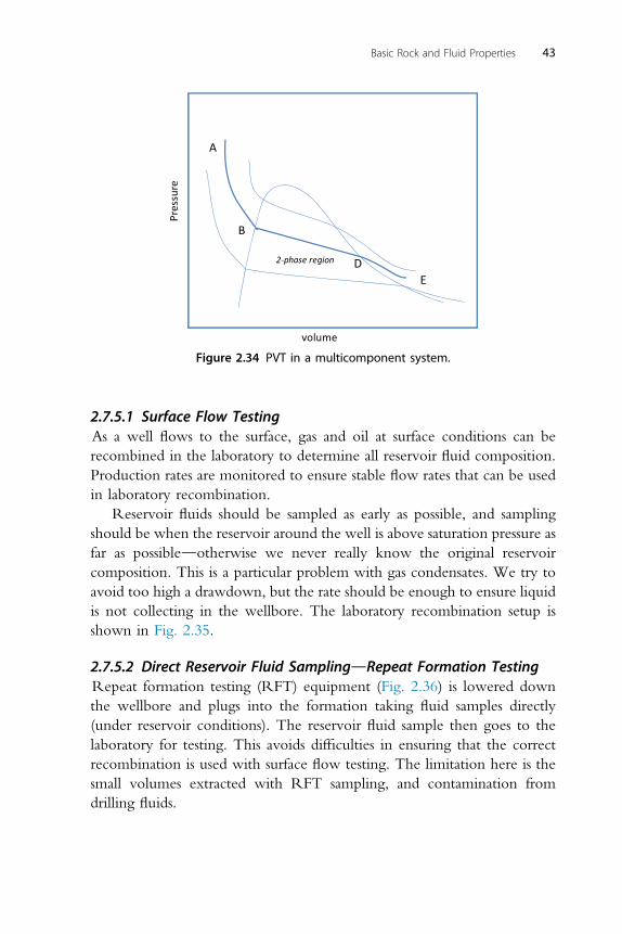
For a multicomponent system, the position is similar, except that as we gofrom liquid to gas expansion is accompanied by a decrease in pressure (seeFig. 2.34).
2.7.5 Obtaining Representative Reservoir Fluid SamplesReservoir fluids are sampled in two ways to obtain representative samplesof the original reservoir fluid.
→E
RU
SS
ER
P
erusserP
Volume
Critical Point
SOLI
D-L
IQU
IDSOLID
LIQUID
CRITICAL
POINT
GAS
T< Tc
TwTc
N
T>Tc Single Phase
A C
P
M
E
B D
Two Phase RegionBu
bble
Poi
nt
Cur
ve
Dew Point Curve
VAPORSOLID-VAPORSPECIFIC VOLUME → TEMPERATURE →
TRIPLE LINE
LIQUID-VAPOR
Figure 2.33 Single-component PVT diagrams.
42 Fundamentals of Applied Reservoir Engineering
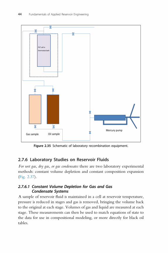
2.7.5.1 Surface Flow TestingAs a well flows to the surface, gas and oil at surface conditions can berecombined in the laboratory to determine all reservoir fluid composition.Production rates are monitored to ensure stable flow rates that can be usedin laboratory recombination.
Reservoir fluids should be sampled as early as possible, and samplingshould be when the reservoir around the well is above saturation pressure asfar as possibledotherwise we never really know the original reservoircomposition. This is a particular problem with gas condensates. We try toavoid too high a drawdown, but the rate should be enough to ensure liquidis not collecting in the wellbore. The laboratory recombination setup isshown in Fig. 2.35.
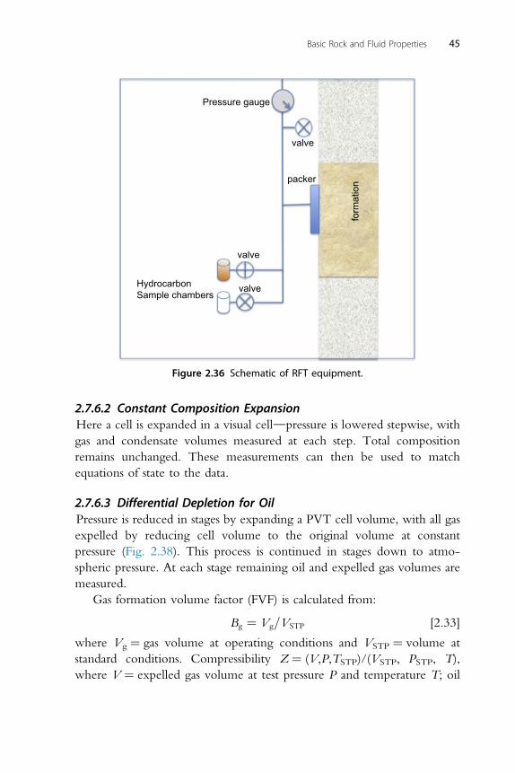
2.7.5.2 Direct Reservoir Fluid SamplingdRepeat Formation TestingRepeat formation testing (RFT) equipment (Fig. 2.36) is lowered downthe wellbore and plugs into the formation taking fluid samples directly(under reservoir conditions). The reservoir fluid sample then goes to thelaboratory for testing. This avoids difficulties in ensuring that the correctrecombination is used with surface flow testing. The limitation here is thesmall volumes extracted with RFT sampling, and contamination fromdrilling fluids.
volume
2-phase region
A
B
DE
Pres
sure
Figure 2.34 PVT in a multicomponent system.
Basic Rock and Fluid Properties 43
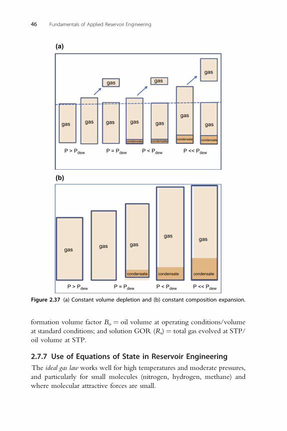
2.7.6 Laboratory Studies on Reservoir FluidsFor wet gas, dry gas, or gas condensates there are two laboratory experimentalmethods: constant volume depletion and constant composition expansion(Fig. 2.37).
2.7.6.1 Constant Volume Depletion for Gas and GasCondensate Systems
A sample of reservoir fluid is maintained in a cell at reservoir temperature,pressure is reduced in stages and gas is removed, bringing the volume backto the original at each stage. Volumes of gas and liquid are measured at eachstage. These measurements can then be used to match equations of state tothe data for use in compositional modeling, or more directly for black oiltables.
PVT
Mercury pumpGas sample Oil sample
PVT cell in
thermostat bath
Figure 2.35 Schematic of laboratory recombination equipment.
44 Fundamentals of Applied Reservoir Engineering
2.7.6.2 Constant Composition ExpansionHere a cell is expanded in a visual celldpressure is lowered stepwise, withgas and condensate volumes measured at each step. Total compositionremains unchanged. These measurements can then be used to matchequations of state to the data.
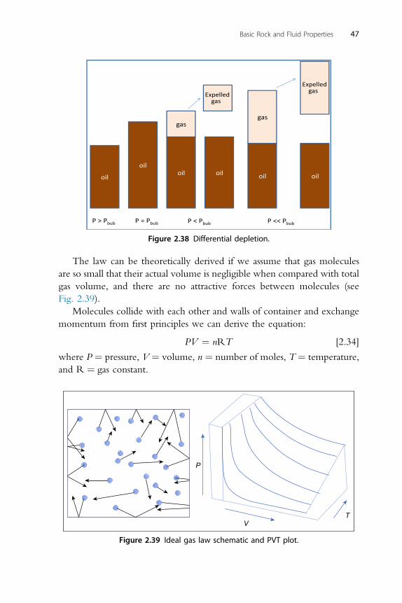
2.7.6.3 Differential Depletion for OilPressure is reduced in stages by expanding a PVT cell volume, with all gasexpelled by reducing cell volume to the original volume at constantpressure (Fig. 2.38). This process is continued in stages down to atmo-spheric pressure. At each stage remaining oil and expelled gas volumes aremeasured.
Gas formation volume factor (FVF) is calculated from:
Bg ¼ Vg=VSTP [2.33]
where Vg ¼ gas volume at operating conditions and VSTP ¼ volume atstandard conditions. Compressibility Z ¼ (V,P,TSTP)/(VSTP, PSTP, T),where V ¼ expelled gas volume at test pressure P and temperature T; oil
Pressure gauge
valve
valve
valve
HydrocarbonSample chambers
packer
form
atio
n
Figure 2.36 Schematic of RFT equipment.
Basic Rock and Fluid Properties 45
formation volume factor Bo ¼ oil volume at operating conditions/volumeat standard conditions; and solution GOR (Rs) ¼ total gas evolved at STP/oil volume at STP.
2.7.7 Use of Equations of State in Reservoir EngineeringThe ideal gas law works well for high temperatures and moderate pressures,and particularly for small molecules (nitrogen, hydrogen, methane) andwhere molecular attractive forces are small.
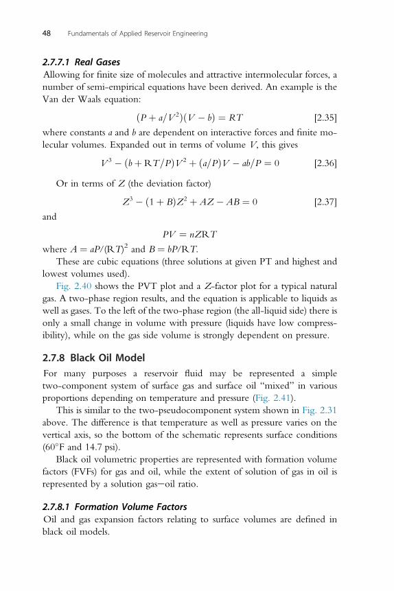
The law can be theoretically derived if we assume that gas moleculesare so small that their actual volume is negligible when compared with totalgas volume, and there are no attractive forces between molecules (seeFig. 2.39).
Molecules collide with each other and walls of container and exchangemomentum from first principles we can derive the equation:
PV ¼ nRT [2.34]
where P ¼ pressure, V ¼ volume, n ¼ number of moles, T ¼ temperature,and R ¼ gas constant.
oil
oiloil oil
gas
Expelledgas
oil
gas
Expelledgas
oil
P > Pbub P < Pbub P << PbubP = Pbub
Figure 2.38 Differential depletion.
P
VT
Figure 2.39 Ideal gas law schematic and PVT plot.
Basic Rock and Fluid Properties 47
2.7.7.1 Real GasesAllowing for finite size of molecules and attractive intermolecular forces, anumber of semi-empirical equations have been derived. An example is theVan der Waals equation:
ðP þ a=V 2ÞðV � bÞ ¼ RT [2.35]
where constants a and b are dependent on interactive forces and finite mo-lecular volumes. Expanded out in terms of volume V, this gives
V 3 � ðbþRT=PÞV 2 þ ða=PÞV � ab=P ¼ 0 [2.36]
Or in terms of Z (the deviation factor)
Z3 � ð1þ BÞZ2 þ AZ � AB ¼ 0 [2.37]
and
PV ¼ nZRT
where A ¼ aP/(RT)2 and B ¼ bP/RT.These are cubic equations (three solutions at given PT and highest and
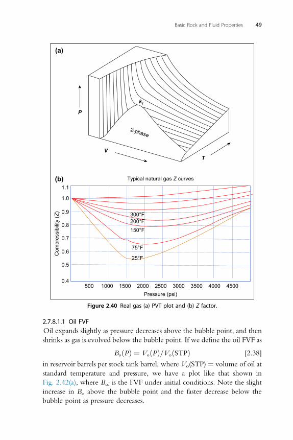
lowest volumes used).Fig. 2.40 shows the PVT plot and a Z-factor plot for a typical natural
gas. A two-phase region results, and the equation is applicable to liquids aswell as gases. To the left of the two-phase region (the all-liquid side) there isonly a small change in volume with pressure (liquids have low compress-ibility), while on the gas side volume is strongly dependent on pressure.
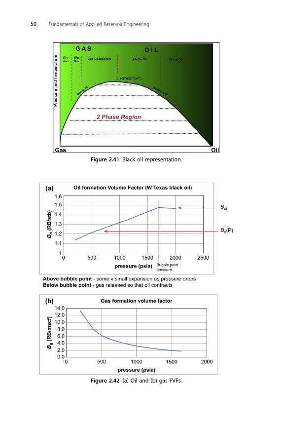
2.7.8 Black Oil ModelFor many purposes a reservoir fluid may be represented a simpletwo-component system of surface gas and surface oil “mixed” in variousproportions depending on temperature and pressure (Fig. 2.41).
This is similar to the two-pseudocomponent system shown in Fig. 2.31above. The difference is that temperature as well as pressure varies on thevertical axis, so the bottom of the schematic represents surface conditions(60�F and 14.7 psi).
Black oil volumetric properties are represented with formation volumefactors (FVFs) for gas and oil, while the extent of solution of gas in oil isrepresented by a solution gaseoil ratio.
2.7.8.1 Formation Volume FactorsOil and gas expansion factors relating to surface volumes are defined inblack oil models.
48 Fundamentals of Applied Reservoir Engineering
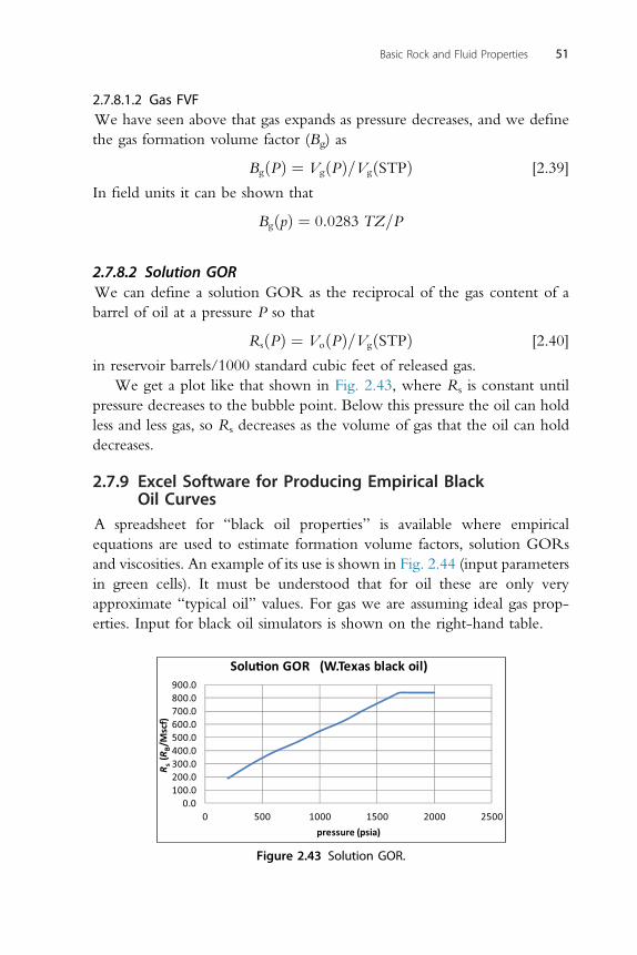
2.7.8.1.1 Oil FVFOil expands slightly as pressure decreases above the bubble point, and thenshrinks as gas is evolved below the bubble point. If we define the oil FVF as
BoðPÞ ¼ VoðPÞ=VoðSTPÞ [2.38]
in reservoir barrels per stock tank barrel, where Vo(STP) ¼ volume of oil atstandard temperature and pressure, we have a plot like that shown inFig. 2.42(a), where Boi is the FVF under initial conditions. Note the slightincrease in Bo above the bubble point and the faster decrease below thebubble point as pressure decreases.
(a)
(b)1.1
300°F200°F150°F
75°F
25°F
1.0
0.9
0.8
0.7
0.6
0.5
0.4500 1000
Com
pres
sibi
lity
(Z)
1500 2000 2500Pressure (psi)
3000 3500 4000 4500
P
kr
VT
2-phase
Typical natural gas Z curves
Figure 2.40 Real gas (a) PVT plot and (b) Z factor.
Basic Rock and Fluid Properties 49
Figure 2.41 Black oil representation.
14.0
(a)
(b)
12.010.0
8.06.04.02.00.0
0 500 1000pressure (psia)
1500 2000
Gas formation volume factor
Oil formation Volume Factor (W Texas black oil) 1.61.5
1.4
1.3
1.2
1.1
10 500
Above bubble point - some v small expansion as pressure dropsBelow bubble point - gas released so that oil contracts
Bo
(RB
/stb
)B
g (R
B/m
scf)
1000 1500Bubble pointpressure
pressure (psia)2000 2500
Bo(P)
Boi
Figure 2.42 (a) Oil and (b) gas FVFs.
50 Fundamentals of Applied Reservoir Engineering
2.7.8.1.2 Gas FVFWe have seen above that gas expands as pressure decreases, and we definethe gas formation volume factor (Bg) as
BgðPÞ ¼ VgðPÞ=VgðSTPÞ [2.39]
In field units it can be shown that
BgðpÞ ¼ 0:0283 TZ=P
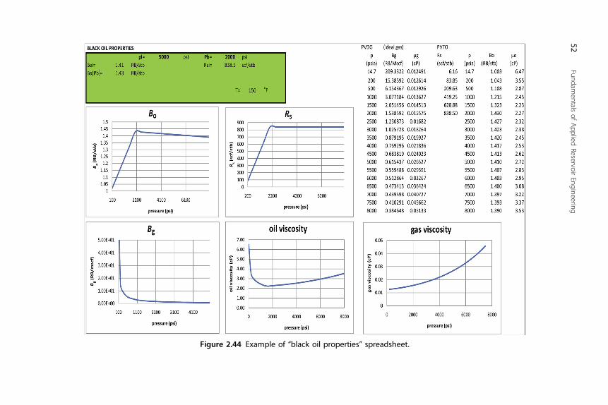
2.7.8.2 Solution GORWe can define a solution GOR as the reciprocal of the gas content of abarrel of oil at a pressure P so that
RsðPÞ ¼ VoðPÞ=VgðSTPÞ [2.40]
in reservoir barrels/1000 standard cubic feet of released gas.We get a plot like that shown in Fig. 2.43, where Rs is constant until
pressure decreases to the bubble point. Below this pressure the oil can holdless and less gas, so Rs decreases as the volume of gas that the oil can holddecreases.
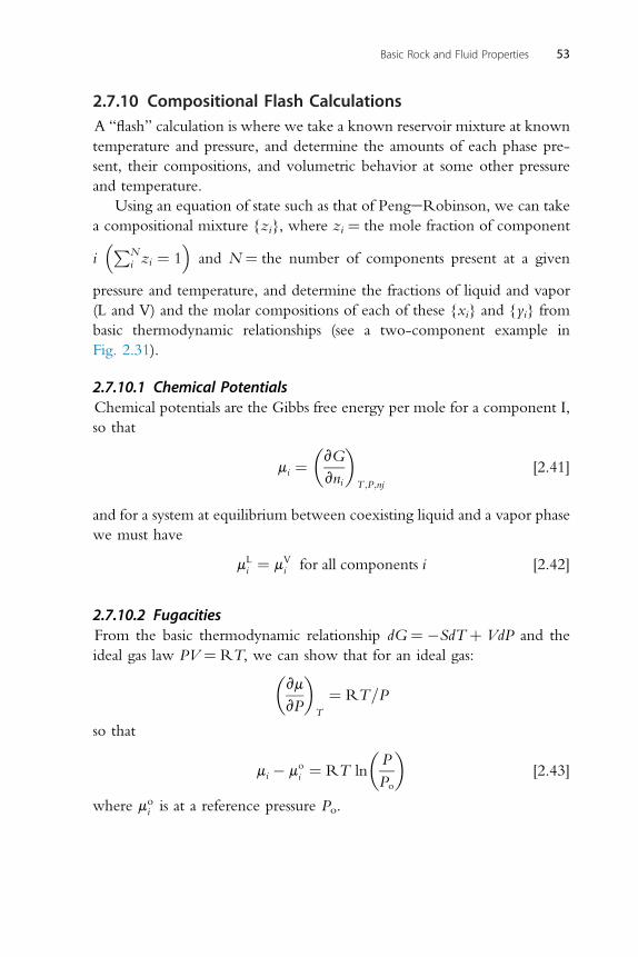
2.7.9 Excel Software for Producing Empirical BlackOil Curves
A spreadsheet for “black oil properties” is available where empiricalequations are used to estimate formation volume factors, solution GORsand viscosities. An example of its use is shown in Fig. 2.44 (input parametersin green cells). It must be understood that for oil these are only veryapproximate “typical oil” values. For gas we are assuming ideal gas prop-erties. Input for black oil simulators is shown on the right-hand table.
0.0100.0200.0300.0400.0500.0600.0700.0800.0900.0
0 500 1000 1500 2000 2500
R s(R
B/M
scf)
pressure (psia)
Solu�on GOR (W.Texas black oil)
Figure 2.43 Solution GOR.
Basic Rock and Fluid Properties 51
Figure 2.44 Example of “black oil properties” spreadsheet.
52Fundam
entalsof
Applied
ReservoirEngineering
2.7.10 Compositional Flash CalculationsA “flash” calculation is where we take a known reservoir mixture at knowntemperature and pressure, and determine the amounts of each phase pre-sent, their compositions, and volumetric behavior at some other pressureand temperature.
Using an equation of state such as that of PengeRobinson, we can takea compositional mixture {zi}, where zi ¼ the mole fraction of component
i�PN
i zi ¼ 1�
and N ¼ the number of components present at a given
pressure and temperature, and determine the fractions of liquid and vapor(L and V) and the molar compositions of each of these {xi} and {yi} frombasic thermodynamic relationships (see a two-component example inFig. 2.31).
2.7.10.1 Chemical PotentialsChemical potentials are the Gibbs free energy per mole for a component I,so that
mi ¼vGvni
T ;P;nj
[2.41]
and for a system at equilibrium between coexisting liquid and a vapor phasewe must have
mLi ¼ mV
i for all components i [2.42]
2.7.10.2 FugacitiesFrom the basic thermodynamic relationship dG ¼ �SdT þ VdP and theideal gas law PV ¼ RT, we can show that for an ideal gas:
vm
vP
T
¼ RT=P
so that
mi � moi ¼ RT ln
PPo
[2.43]
where moi is at a reference pressure Po.
Basic Rock and Fluid Properties 53
2.7.10.3 For a Real GasWe can define a “corrected pressure” function fi (for a real gas), calledfugacity:
mi � moi ¼ RT ln
fif oi
[2.44]
A definition of fugacity is thus as a measure of nonideality. SincemLi ¼ mV
i , it can be shown that similarly, f Li ¼ f Vi for all components i inequilibrium.
We now define a fugacity coefficient 4i,4i ¼ fi/P$zi (where zi ¼ mole fraction of component i)4i / 1 when P / 0.From fundamental thermodynamic relationships,
lnð4iÞ ¼1
RT
Z (vPvni
T ;V ;nj
�RT=V
)dV � ln Z [2.45]
Thus once we have a function for Z, we can derive fugacity for acomponent i in liquid and vapor phases from ZL and ZV which come fromthe equation of state.
Since
f Vi ¼ yiP4Vi and f Li ¼ xiP4
Li
if we define a ratio of mole fraction of i in the liquid phase to that in thevapor phase:
Ki ¼ yi=xi ¼ 4Li
�4Vi
Now we also have the relationships L þ V ¼ 1 and zi ¼ xi$L þ yi$V.Using all of the above, the iterative “flash” calculation process can be
summarized as detailed in the following subsections.
2.7.10.4 Cubic Equation of State of FormaZ3 þ bZ2 þ cZ þ d ¼ 0
where a, b, c, and d are functions of the critical properties of all componentsand interaction coefficients between components.
Solved to Give PVT RelationshipsThis can also give chemical potentials (and fugacities) of each component ingas and liquid phases (mL
i and mVi ). These must be equal for each component.
54 Fundamentals of Applied Reservoir Engineering
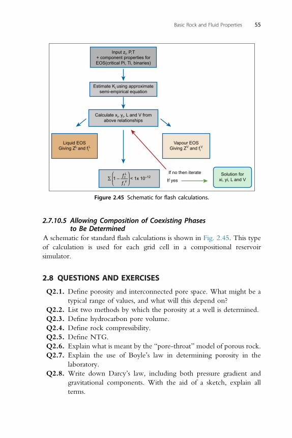
2.7.10.5 Allowing Composition of Coexisting Phasesto Be Determined
A schematic for standard flash calculations is shown in Fig. 2.45. This typeof calculation is used for each grid cell in a compositional reservoirsimulator.
2.8 QUESTIONS AND EXERCISES
Q2.1. Define porosity and interconnected pore space. What might be atypical range of values, and what will this depend on?
Q2.2. List two methods by which the porosity at a well is determined.Q2.3. Define hydrocarbon pore volume.Q2.4. Define rock compressibility.Q2.5. Define NTG.Q2.6. Explain what is meant by the “pore-throat” model of porous rock.Q2.7. Explain the use of Boyle’s law in determining porosity in the
laboratory.Q2.8. Write down Darcy’s law, including both pressure gradient and
gravitational components. With the aid of a sketch, explain allterms.
Estimate Ki using approximatesemi-empirical equation
Calculate xi, yi, L and V fromabove relationships
Vapour EOSGiving ZV and fi
V
Solution forxi, yi, L and V
If no then iterate
Liquid EOSGiving ZL and fi
L
If yes∑ 1 – –— < 1x 10–12ƒtL
ƒtV
⎞⎟⎠
⎛⎜⎝
Figure 2.45 Schematic for flash calculations.
Basic Rock and Fluid Properties 55
Q2.9. Calculate the absolute permeability from laboratory data foran incompressible fluid where A ¼ 12.5 cm2, x ¼ 10 cm,P1 e P2 ¼ 50 psi, Q ¼ 0.05 cm3/s, fluid viscosity ¼ 2.0 cP.
Q2.10. Calculate the absolute permeability from the following laboratorydata for flow of gas across a horizontal core: A ¼ 5.06 cm2,x ¼ 8 cm, P1 ¼ 200 psi, P2 ¼ 195 psi, Q ¼ 23.6 cm3/s, gasviscosity ¼ 0.0178 cP.
Q2.11. Write down Darcy’s law in field units, listing the dimensions ofeach.
Q2.12. For an oilewater system, explain with the aid of a sketch the sig-nificance of the “contact angle.”
Q2.13. Explain with the aid of diagrams what is meant by the terms“drainage” and “imbibition” for an oilewater system (in waterwet material). Sketch both capillary pressure and relative perme-ability curves. To which process would water flooding correspond?
Q2.14. Draw a plot relating oil and water pressures to depth (oilewatersystem with no gas). Relate this to water saturation.
Q2.15. Explain what is meant by effective permeability. Write theDarcy equation for a phase a where more than a single phaseis present.
Q2.16. With the aid of sketches, show the difference you would expect inthe relative permeability curves for “water wet” and “oil wet”systems.
Q2.17. Sketch PT phase envelopes for the following.1. A dry gas.2. A wet gas.3. A gas condensate.4. A heavy oil.Show changing reservoir conditions and changes to surfaceconditions.
Q2.18. Describe, with the aid of simple schematics, the laboratory testsfor constant volume depletion and constant compositionexpansion.
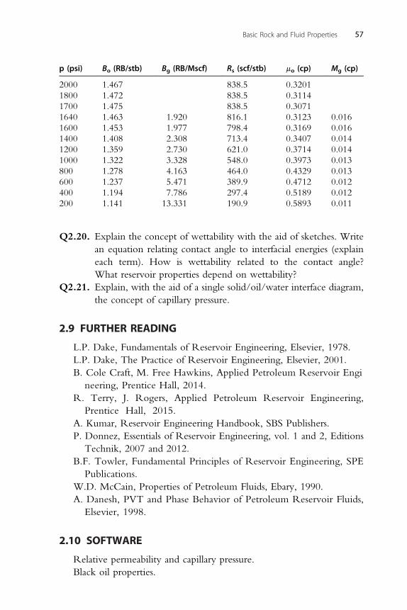
Q2.19. The table below shows laboratory measurements of formation vol-ume factors, solution GOR, and viscosities as functions of pressure.Use a spreadsheet to plot all of these. Identify the bubble-pointpressure for this oil.
56 Fundamentals of Applied Reservoir Engineering
Q2.20. Explain the concept of wettability with the aid of sketches. Writean equation relating contact angle to interfacial energies (explaineach term). How is wettability related to the contact angle?What reservoir properties depend on wettability?
Q2.21. Explain, with the aid of a single solid/oil/water interface diagram,the concept of capillary pressure.
2.9 FURTHER READING
L.P. Dake, Fundamentals of Reservoir Engineering, Elsevier, 1978.L.P. Dake, The Practice of Reservoir Engineering, Elsevier, 2001.B. Cole Craft, M. Free Hawkins, Applied Petroleum Reservoir Engi