82
Chapter 2 Math Fundamentals Part 2 2.4 Kinematics of Mechanisms 2.5 Orientation and Angular Velocity Mobile Robotics - Prof Alonzo Kelly, CMU RI 1

Chapter 2 Math Fundamentals
Part 2 2.4 Kinematics of Mechanisms 2.5 Orientation and Angular Velocity
Mobile Robotics - Prof Alonzo Kelly, CMU RI 1
Outline • 2.4 Kinematics of Mechanisms • 2.5 Orientation and Angular Velocity
Mobile Robotics - Prof Alonzo Kelly, CMU RI 2

Outline • 2.4 Kinematics of Mechanisms
– 2.4.1 Forward Kinematics – 2.4.2 Inverse Kinematics – 2.4.3 Differential Kinematics – Summary
• 2.5 Orientation and Angular Velocity
Mobile Robotics - Prof Alonzo Kelly, CMU RI 3

Definitions • Motion = movement of the whole body thru
space. • Articulation = reconfigures mass without
substantial motion • Attitude = pitch and roll. • Orientation = attitude & (heading or yaw). • Pose = position & orientation
4 Mobile Robotics - Prof Alonzo Kelly, CMU RI
x y ψT
x y z θ φ ψT
4

5 Mobile Robotics - Prof Alonzo Kelly, CMU RI
Task and Joint Space
• For manipulators, joint space is also C Space.
• Manipulators are difficult for operators to control in joint space.
BASE TOOL
Joint Space
Task Space
θ1
θ2
θ3
5

6 Mobile Robotics - Prof Alonzo Kelly, CMU RI
Linear Mapping
• So far, we have used:
• We have considered this to be a linear mapping in r – In part, because the matrix is considered a constant.
Operator or Transform
Input Vector
Output Vector
Task Space Task Space r' T ρ( )r=
r r′

7 Mobile Robotics - Prof Alonzo Kelly, CMU RI
2.4.1.1 Nonlinear Mapping • There is another view of just the T(ρ) part when the
“aligning operations” correspond to real joints:
• This is a nonlinear mapping in ρ. • T is a matrix-valued function of the configuration vector
ρ. • Recall that T can represent the pose of a rigid body (we
saw this in 2D with HTs).
Forward Kinematics
Articulation Variables
Transform T
Task Space Configuration Space
ρ

8 Mobile Robotics - Prof Alonzo Kelly, CMU RI
2.4.1.2 Mechanism Models • Let ρ represent the articulations of a mechanism. • It is convenient to think about the moving axis operations
which align a sequence of frames with each other.
8

9 Mobile Robotics - Prof Alonzo Kelly, CMU RI
Conventional Rules of Forward Kinematics
• 1: Assign embedded frames to the links in sequence such that the operations which move each frame into coincidence with the next are a function of the current joint variable.
• 2: Write the orthogonal operator matrices which correspond to these operations in left to right order.
• This process will generate the matrix that: – A: represents the position and orientation of the last
embedded frame with respect to the first, or equivalently, – B: which converts the coordinates of a point from the last to
the first.
9

10 Mobile Robotics - Prof Alonzo Kelly, CMU RI
2.4.1.3 Denavit-Hartenberg Convention
• A special product of 4 fundamental operators is used as a basic conceptual unit.
• Its still an orthogonal transform so it has the properties of the component transforms, namely: – Operates on points – Converts coordinates – Represents axes of one system wrt another
10
11 Mobile Robotics - Prof Alonzo Kelly, CMU RI
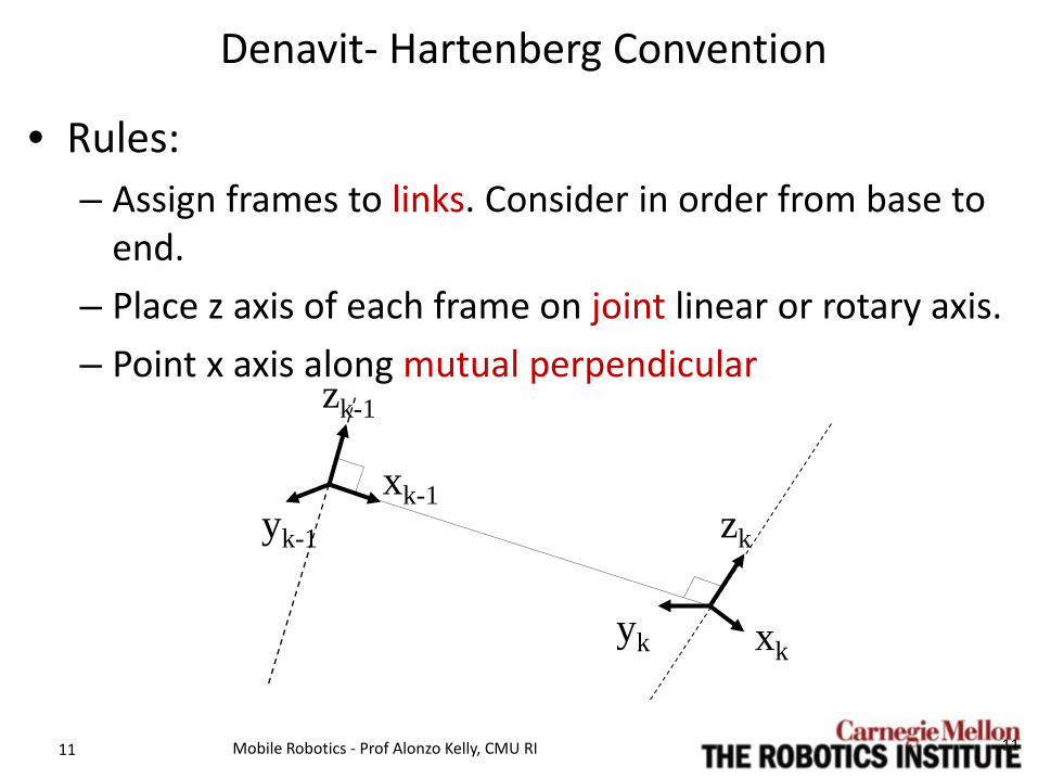
Denavit- Hartenberg Convention
• Rules: – Assign frames to links. Consider in order from base to
end. – Place z axis of each frame on joint linear or rotary axis. – Point x axis along mutual perpendicular
zk-1
yk-1
xk-1 zk
yk xk
11

12 Mobile Robotics - Prof Alonzo Kelly, CMU RI
Denavit- Hartenberg Convention • Move first frame into
coincidence with second thus: – rotate around the xk-1
axis by an angle φk
– translate along the xk-1 axis by a distance uk
– rotate around the new z axis by an angle ψk
– translate along the new z axis by a distance wk
xk-1 φk
zk
zk-1
yk-1
yi
xk-1
zk
xk
yk
yi
ψk
zk
xk
yk
uk wk
How can we get away with just four dof?

Tkk 1– Rotx φk( )Trans uk 0 0, ,( )Rotz ψk( )Trans 0 0 wk, ,( )=
Tkk 1–
1 0 0 00 cφk s– φk 0
0 sφk cφk 0
0 0 0 1
1 0 0 uk
0 1 0 00 0 1 00 0 0 1
cψk s– ψk 0 0
sψk cψk 0 0
0 0 1 00 0 0 1
1 0 0 00 1 0 00 0 1 wk
0 0 0 1
=
Ak Tkk 1–=
cψk s– ψk 0 uk
cφksψk cφkcψk s– φk s– φkwk
sφksψk sφkcψk cφk cφkwk
0 0 0 1
=
14 Mobile Robotics - Prof Alonzo Kelly, CMU RI
Denavit- Hartenberg Convention • Moving axis operations in left to right order:
4 “parameters”

15 Mobile Robotics - Prof Alonzo Kelly, CMU RI
Denavit- Hartenberg Convention
• This matrix has the following interpretations: – It will move a point or rotate a direction by the operator which
describes how frame k is related to frame k-1. – Its columns represent the axes and origin of frame k expressed in
frame k-1 coordinates. – It converts coordinates from frame k to frame k-1.
Special Notation
Ak Tkk 1–=
cψk s– ψk 0 uk
cφksψk cφkcψk s– φk s– φkwk
sφksψk sφkcψk cφk cφkwk
0 0 0 1
=

16 Mobile Robotics - Prof Alonzo Kelly, CMU RI
2.4.1.4 Example: 3 Link Planar Manipulator
Link φ u ψ w 0 0 0 ψ1 0 1 0 L1 ψ2 0 2 0 L2 ψ3 0 3 0 L3 0 0
x0,1
y0,1
ψ1
x2
y2
ψ2 x3
y3
ψ3
y4
x4
L1 L2 L3
0
1 2 3

17 Mobile Robotics - Prof Alonzo Kelly, CMU RI
Example: 3 Link Planar Manipulator
A1
c1 s1– 0 0
s1 c1 0 0
0 0 1 00 0 0 1
= A11–
c1 s1 0 0
s1– c 1 0 0
0 0 1 00 0 0 1
=
A3
c3 s3– 0 L2
s3 c3 0 0
0 0 1 00 0 0 1
= A31–
c3 s3 0 c– 3L2
s3– c3 0 s3L2
0 0 1 00 0 0 1
= A4
1 0 0 L 3
0 1 0 00 0 1 00 0 0 1
= A41–
1 0 0 L– 3
0 1 0 00 0 1 00 0 0 1
=
A2
c 2 s2– 0 L1
s2 c2 0 0
0 0 1 00 0 0 1
= A21–
c 2 s2 0 c 2L1–
s2– c2 0 s2L1
0 0 1 00 0 0 1
=
Ak Tkk 1–=
cψk s– ψk 0 uk
cφksψk cφkcψk s– φk s– φkwk
sφksψk sφkcψk cφk cφkwk
0 0 0 1
=

18 Mobile Robotics - Prof Alonzo Kelly, CMU RI
Example: 3 Link Planar Manipulator T4
0 T10 T2
1T32T4
3 A 1A2A3A4= =
T40
c1 s1– 0 0
s1 c 1 0 0
0 0 1 00 0 0 1
c2 s2– 0 L1
s2 c2 0 0
0 0 1 00 0 0 1
c 3 s3– 0 L2
s3 c3 0 0
0 0 1 00 0 0 1
1 0 0 L3
0 1 0 00 0 1 00 0 0 1
=
T40
c 123 s123– 0 c123L3 c 12L2 c 1L1+ +( )
s123 c123 0 s123L3 s12L2 s1L1+ +( )
0 0 1 00 0 0 1
=
position orientation
A Completely General Forward Kinematics Solution!

Outline • 2.4 Kinematics of Mechanisms
– 2.4.1 Forward Kinematics – 2.4.2 Inverse Kinematics – 2.4.3 Differential Kinematics – Summary
• 2.5 Orientation and Angular Velocity
Mobile Robotics - Prof Alonzo Kelly, CMU RI 19
20 Mobile Robotics - Prof Alonzo Kelly, CMU RI
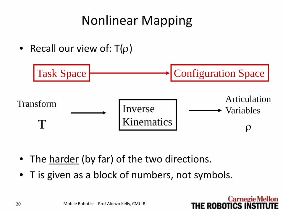
Nonlinear Mapping
• Recall our view of: T(ρ)
• The harder (by far) of the two directions. • T is given as a block of numbers, not symbols.
Inverse Kinematics
Articulation Variables
Transform
T
Configuration Space Task Space
ρ

Kinematics
Mobile Robotics - Prof Alonzo Kelly, CMU RI 21
Base
Tool
Base
Tool
Shoulder Elbow Wrist

23 Mobile Robotics - Prof Alonzo Kelly, CMU RI
2.4.2.1 Existence and Uniqueness • Existence
– Nonlinear equations need not be solveable.
• Uniqueness – There is no rule requiring only one answer. – E.g. tanθ = θ
θ
tanθ
π/2 3π/2 5π/2 7π/2
θ
23

24 Mobile Robotics - Prof Alonzo Kelly, CMU RI
Existence • Nonlinear equations need not be solveable.
Goal
24

25 Mobile Robotics - Prof Alonzo Kelly, CMU RI
Uniqueness • There is no rule requiring only one answer.
Goal
25

26 Mobile Robotics - Prof Alonzo Kelly, CMU RI
2.4.2.2 Technique • Rewrite equations in multiple ways in order to isolate unknowns.
– No new info generated, its just algebra.
T40 A1A2A3A4=
A11– T4
0 A2A3A4=
A21– A1
1– T40 A3A4=
A31– A2
1– A11– T4
0 A4=
A41– A3
1– A21– A1
1– T40 I=
T40 A1A2A3A4=
T40A4
1– A1A2A3=
T40A4
1– A31– A1A2=
T40A4
1– A31– A2
1– A1=
T40A4
1– A31– A2
1– A11– I=
Premultiply Postmultiply
26

27 Mobile Robotics - Prof Alonzo Kelly, CMU RI
2.4.2.3 Example: 3 Link Planar Manipulator • Account for known quantities. • This is a 2D problem, so…
T40
r11 r12 r13 px
r21 r22 r23 py
r31 r32 r33 pz
0 0 0 1
r11 r12 0 px
r21 r22 0 py
0 0 1 00 0 0 1
= =
27

28 Mobile Robotics - Prof Alonzo Kelly, CMU RI
Example: 3 Link Planar Manipulator
• From the (1,1) and (2,1) elements we have:
T40 A1A2A3A4=
r11 r12 0 px
r21 r22 0 py
0 0 1 00 0 0 1
c 123 s123– 0 c123L3 c 12L2 c 1L1+ +( )
s123 c123 0 s123L3 s12L2 s1L1+ +( )
0 0 1 00 0 0 1
=
ψ123 2 r21 r11,( )atan=
28

r11 r 12 0 r11L3– px+
r21 r 22 0 r21L3– py+
0 0 1 00 0 0 1
c123 s123– 0 c12 L2 c1L1+
s123 c123 0 s12 L2 s1L1+
0 0 1 00 0 0 1
=
29 Mobile Robotics - Prof Alonzo Kelly, CMU RI
Example: 3 Link Planar Manipulator
• From the (1,4) and (2,4) elements we have:
T40A4
1– A1 A2A3=r11 r 12 0 r11L3– px+
r21 r 22 0 r21L3– py+
0 0 1 00 0 0 1
c123 s123– 0 c1 c2L2 L1+( ) s1 s2L2( )–
s123 c123 0 s1 c 2L2 L1+( ) c1 s2L2( )+
0 0 1 00 0 0 1
=
k1 r11L3– px+ c12 L2 c1 L1+= =
k2 r21L3– py+ s12 L2 s1L1+= =
29

30 Mobile Robotics - Prof Alonzo Kelly, CMU RI
Example: 3 Link Planar Manipulator • Repeat from last slide: from the (1,4) and (2,4) elements we have:
• Square and add (eliminates θ1) to yield:
• Or:
• Rearranging gives the answer:
• Each solution gives different values for the other two angles.
k1 r11L3– px+ c12 L2 c1 L1+= =
k2 r21L3– py+ s12 L2 s1L1+= =
k12 k2
2+ L22 L1
2 2L2L1 c1c12 s1s12+( )+ +=
ψ2k1
2 k22+( ) L2
2 L12+( )–
2L2 L1----------------------------------------------------acos=
cosψ2 k12 k2
2+ L22 L1
2 2L2L1c2+ +=
30
31 Mobile Robotics - Prof Alonzo Kelly, CMU RI
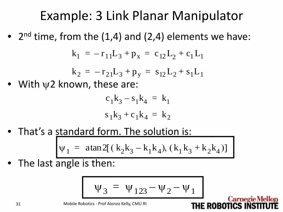
Example: 3 Link Planar Manipulator • 2nd time, from the (1,4) and (2,4) elements we have:
• With ψ2 known, these are:
• That’s a standard form. The solution is:
• The last angle is then:
k1 r11L3– px+ c12 L2 c1 L1+= =
k2 r21L3– py+ s12 L2 s1L1+= =
c1k3 s1k4– k1=
s 1k3 c1k4+ k2=
ψ1 2atan k2k3 k1k4–( ) k1 k3 k2k4+( ),[ ]=
ψ3 ψ123 ψ2 ψ1––=31

32 Mobile Robotics - Prof Alonzo Kelly, CMU RI
That’s PRETTY AWESOME!
Goal
ψ123 2 r21 r11,( )atan=
ψ2k1
2 k22+( ) L2
2 L12+( )–
2L2 L1----------------------------------------------------acos=
ψ1 2atan k2k3 k1k4–( ) k1 k3 k2k4+( ),[ ]=
ψ3 ψ123 ψ2 ψ1––=
32

33 Mobile Robotics - Prof Alonzo Kelly, CMU RI
• Occurs very frequently:
• Isolate tangent:
• Clearly:
2.4.2.4 Standard Forms: Explicit Tangent
a cn=b sn=
ψn 2 b a,( )atan=
a b
Why do we need two equations for one unknown?
33

34 Mobile Robotics - Prof Alonzo Kelly, CMU RI
2.4.2.4 Standard Forms: Point Symmetric • Occurs as:
• Isolate tangent:
• Clearly:
a b
sna cnb– 0=
ψn 2 b a,( )atan=
ψn 2 b– a–,( )atan=
sncn----- b
a---=
Why two solutions?
34

35 Mobile Robotics - Prof Alonzo Kelly, CMU RI
2.4.2.4 Standard Forms: Line Symmetric • Occurs as:
• Trig substitution:
• Leads to:
• So: • Solution
a b
sna cn b– c=
a r θ( )cos=b r θ( )sin=
s θ ψn–( ) c r⁄=
r
c θ ψn–( ) sqrt 1 c r⁄( )2–( )±=
ψn 2 b a,( ) 2 c sqr t r2 c2–( )±,[ ]atan–atan=35

36 Mobile Robotics - Prof Alonzo Kelly, CMU RI
Inverse Kinematics of a DH HT?
Inverse Kinematics
Articulation Variables
Transform T ρ
r11 r12 r13 px
r21 r22 r23 py
r31 r32 r33 pz
0 0 0 1
cψ i s– ψi 0 ui
cφisψ i cφicψi s– φi s– φi wi
sφi sψi s φicψi cφi cφiwi
0 0 0 1
=
36

37 Mobile Robotics - Prof Alonzo Kelly, CMU RI
Inverse Kinematics of a DH HT?
• Translation part is easy: ui px=
wi py2 pz
2+=
r11 r12 r13 px
r21 r22 r23 py
r31 r32 r33 pz
0 0 0 1
cψ i s– ψi 0 ui
cφisψ i cφicψi s– φi s– φi wi
sφi sψi s φicψi cφi cφiwi
0 0 0 1
=
Tba = Rotx ϕi Trans(ui, 0,0)Rotz ψi Trans(wi, 0,0)
37
38 Mobile Robotics - Prof Alonzo Kelly, CMU RI
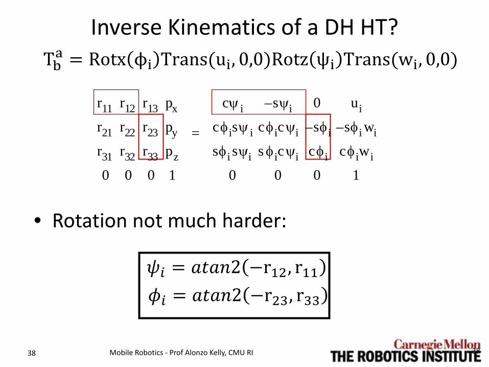
Inverse Kinematics of a DH HT?
• Rotation not much harder:
r11 r12 r13 px
r21 r22 r23 py
r31 r32 r33 pz
0 0 0 1
cψ i s– ψi 0 ui
cφisψ i cφicψi s– φi s– φi wi
sφi sψi s φicψi cφi cφiwi
0 0 0 1
=
Tba = Rotx ϕi Trans(ui, 0,0)Rotz ψi Trans(wi, 0,0)
𝜓𝜓𝑖𝑖 = 𝑎𝑎𝑎𝑎𝑎𝑎𝑎𝑎𝑎 −r12, r11 𝜙𝜙𝑖𝑖 = 𝑎𝑎𝑎𝑎𝑎𝑎𝑎𝑎𝑎 −r23, r33
38

Outline • 2.4 Kinematics of Mechanisms
– 2.4.1 Forward Kinematics – 2.4.2 Inverse Kinematics – 2.4.3 Differential Kinematics – Summary
• 2.5 Orientation and Angular Velocity
Mobile Robotics - Prof Alonzo Kelly, CMU RI 39
40 Mobile Robotics - Prof Alonzo Kelly, CMU RI
Differential Kinematics • Studies the derivatives (first order behavior) of
kinematic models. • Use Jacobians (multidimensional derivatives) to
do this. • Use them for:
– Resolved rate control – Sensitivity analysis – Uncertainty propagation – Static force transformation
40

41 Mobile Robotics - Prof Alonzo Kelly, CMU RI
Derivatives of Fundamental Operators
x
y
z θ
• Note capital R in Rotx().
Rotx φ( )
1 0 0 00 cφ sφ– 00 sφ cφ 00 0 0 1
=
φ∂∂ Rotx φ( )
0 0 0 00 s– φ c– φ 00 cφ s– φ 00 0 0 0
=
41

42 Mobile Robotics - Prof Alonzo Kelly, CMU RI
Derivatives of Fundamental Operators
u∂∂ T rans u v w, ,( )
0 0 0 10 0 0 00 0 0 00 0 0 0
=
v∂∂ Trans u v w, ,( )
0 0 0 00 0 0 10 0 0 00 0 0 0
=
w∂∂ Trans u v w, ,( )
0 0 0 00 0 0 00 0 0 10 0 0 0
=
φ∂∂ Rotx φ( )
0 0 0 00 s– φ c– φ 00 cφ s– φ 00 0 0 0
=
θ∂∂ Roty θ( )
s– θ 0 cθ 00 0 0 0c– θ 0 s– θ 00 0 0 0
=
ψ∂∂ Rotz ψ( )
s– ψ c– ψ 0 0cψ s– ψ 0 00 0 0 00 0 0 0
=
42

43 Mobile Robotics - Prof Alonzo Kelly, CMU RI
2.4.3.2 Mechanism Jacobian
• How much does end effector move if I tweak this angle 1 degree?
43

44 Mobile Robotics - Prof Alonzo Kelly, CMU RI
2.4.3.2 Mechanism Jacobian
• Recall a Jacobian…. • If:
• Then:
• Basic use:
x and q can be anything
44

45 Mobile Robotics - Prof Alonzo Kelly, CMU RI
Resolved Rate Control
• By the Chain Rule of Differentiation:
• This is just:
• Suppose x is the position of the end effector. This is: – Nonlinear in joint variables – Linear in the joint rates!
What does that imply?
45

46 Mobile Robotics - Prof Alonzo Kelly, CMU RI
Resolved Rate Control
• Direct mapping from desired velocity onto joint rates!
• Singularity (infinite joint rates) occurs: – at points where two different inverse kinematic solutions
converge – when joint axes become aligned or parallel – when the boundaries of the workspace are reached
v
q· J q( ) 1– x·=

47 Mobile Robotics - Prof Alonzo Kelly, CMU RI
2.4.3.5 Jacobian Determinant
• Relates differential volumes in task space to differential volumes in configuration space. – Used in calculus for double, triple, etc integrals.
• We will use this later to figure out when landmarks are in unfavorable configurations for navigation.
dx1dx2…dxn( ) J dq1dq2 …dqm( )=
|J| dx1
dx2
dx3 dq1
dq2
dq3
48 Mobile Robotics - Prof Alonzo Kelly, CMU RI
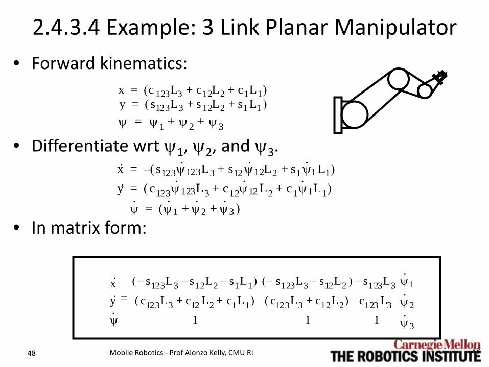
2.4.3.4 Example: 3 Link Planar Manipulator • Forward kinematics:
• Differentiate wrt ψ1, ψ2, and ψ3.
• In matrix form:
x c 123L3 c12L2 c1L1+ +( )=y s123L3 s 12L2 s1 L1+ +( )=ψ ψ1 ψ2 ψ3+ +=
x· s123ψ· 123L3 s12 ψ· 12L2 s1 ψ· 1 L1+ +( )–=y· c123ψ· 123L3 c12ψ
·12 L2 c1ψ· 1L1+ +( )=
ψ· ψ· 1 ψ· 2 ψ· 3+ +( )=
x·
y·
ψ·
s123L3– s12L2– s1L1–( ) s123L3– s12L2–( ) s123L3–
c123L3 c12 L2 c1L1+ +( ) c123L3 c12L2+( ) c123 L3
1 1 1
ψ· 1
ψ· 2
ψ· 3
=
48

Outline • 2.4 Kinematics of Mechanisms
– 2.4.1 Forward Kinematics – 2.4.2 Inverse Kinematics – 2.4.3 Differential Kinematics – Summary
• 2.5 Orientation and Angular Velocity
Mobile Robotics - Prof Alonzo Kelly, CMU RI 49
50 Mobile Robotics - Prof Alonzo Kelly, CMU RI
Summary • We can model the forward kinematics of
mechanisms by – embedding frames in rigid bodies – employing the fundamental orthogonal
operator matrices – employing a few rules for writing them in the
right order to represent a mechanism. • The DH convention consists of a special
compound orthogonal transform and a few rules for orienting the link frames. – These can be used just like the fundamental
orthogonal operator matrices to do forward kinematics.
50

51 Mobile Robotics - Prof Alonzo Kelly, CMU RI
Summary • Inverse kinematics requires more skill and
relies on rewriting the forward equations in an attempt to isolate unknowns.
• Various derivatives of kinematic transforms can be taken and each has some use.
51

Outline • 2.4 Kinematics of Mechanisms • 2.5 Orientation and Angular Velocity
– 2.5.1 Orientation in Euler Angle Form – 2.5.2 Angular Rates and Small Angles – 2.5.3 Angular Velocity and Orientation Rates in Euler
Angle Form – 2.5.4 Angular Velocity and Orientation Rates in Angle-
Axis Form – 2.5.5 Summary
Mobile Robotics - Prof Alonzo Kelly, CMU RI 52
53 Mobile Robotics - Prof Alonzo Kelly, CMU RI
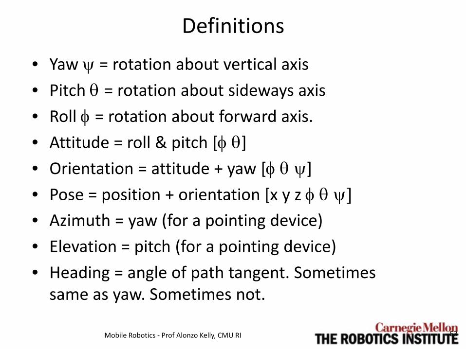
Definitions
• Yaw ψ = rotation about vertical axis • Pitch θ = rotation about sideways axis • Roll φ = rotation about forward axis. • Attitude = roll & pitch [φ θ] • Orientation = attitude + yaw [φ θ ψ] • Pose = position + orientation [x y z φ θ ψ] • Azimuth = yaw (for a pointing device) • Elevation = pitch (for a pointing device) • Heading = angle of path tangent. Sometimes
same as yaw. Sometimes not.

54 Mobile Robotics - Prof Alonzo Kelly, CMU RI
Definitions • Pose = position & orientation
• In 2D:
• In 3D:
x y ψT
x y z θ φ ψT

55 Mobile Robotics - Prof Alonzo Kelly, CMU RI
2.5.1.1. Axis Conventions • Aerospace:
• Ground Vehicles (here at least):
z yaw
x roll y
pitch
z yaw
x roll
y pitch

56 Mobile Robotics - Prof Alonzo Kelly, CMU RI
2.5.1.2 Frame Assignment
Letter Name
n,w Navigation, world
w world
p positioner
b,v body, vehicle
h head
s sensor
c wheel contact
𝑥𝑥 𝑦𝑦
𝑎𝑎,𝑤𝑤
𝑝𝑝
𝑐𝑐
𝑏𝑏, 𝑣𝑣 ℎ 𝑠𝑠
𝑥𝑥 𝑧𝑧
𝑐𝑐
𝑝𝑝
𝑏𝑏, 𝑣𝑣
ℎ
𝑎𝑎,𝑤𝑤

57 Mobile Robotics - Prof Alonzo Kelly, CMU RI
2.5.1.3 The RPY Transform • Similar to DH Matrix but encodes 6 dof: • Aligning operations that move ‘a’ into coincidence
with ‘b’: – translate along the (x,y,z) axes of frame ‘a’ by (u,v,w)
until its origin coincides with that of frame ‘b’ – rotate about the new z axis by an angle ψ called yaw – rotate about the new y axis by an angle θ called pitch – rotate about the new x axis by an angle φ called roll

RPY Forward Kinematics
58 Mobile Robotics - Prof Alonzo Kelly, CMU RI
Tba Trans u v w, ,( )Rotz ψ( )Roty θ( )Rotx φ( )=
Tba
1 0 0 u0 1 0 v0 0 1 w0 0 0 1
cψ s– ψ 0 0sψ cψ 0 00 0 1 00 0 0 1
cθ 0 sθ 00 1 0 0s– θ 0 cθ 00 0 0 1
1 0 0 00 cφ s– φ 00 s φ cφ 00 0 0 1
=
Tba
cψcθ cψsθ sφ sψcφ–( ) cψsθcφ sψsφ+( ) usψcθ sψsθsφ cψcφ+( ) sψsθ cφ cψsφ–( ) v
s θ– cθ sφ cθcφ w0 0 0 1
=

r11 r12 r13 px
r21 r22 r23 py
r31 r32 r33 pz
0 0 0 1
cψcθ cψsθsφ sψcφ–( ) cψsθcφ sψsφ+( ) usψcθ sψsθsφ cψcφ+( ) sψsθcφ cψsφ–( ) v
sθ– cθsφ cθcφ w0 0 0 1
=
59 Mobile Robotics - Prof Alonzo Kelly, CMU RI
2.5.1.4 RPY Transform Inverse Kinematics Tb
a Trans u v w, ,( )Ro tz ψ( )Rotx θ( )Roty φ( )=
body x axis in world
• Yaw can be determined from a vector aligned with the body x axis expressed in world coordinates .
• Is there another solution? • Only if there are 2 solutions for θ.
• What if cθ is zero?
ψ 2 r21 r11,( )atan=
60 Mobile Robotics - Prof Alonzo Kelly, CMU RI
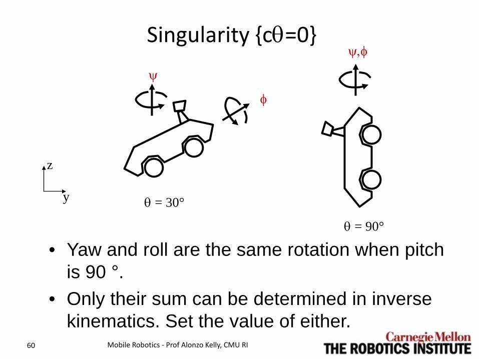
Singularity cθ=0
• Yaw and roll are the same rotation when pitch is 90 °.
• Only their sum can be determined in inverse kinematics. Set the value of either.
z
y
ψ
φ
ψ,φ
θ = 30°
θ = 90°

Rotz ψ( )[ ] 1– Trans u v w, ,( )[ ] 1– Tba Roty θ( )Rotx φ( )=
r11cψ r21sψ+( ) r12 cψ r22 sψ+( ) r13 cψ r23 sψ+( ) 0
r– 11sψ r21cψ+( ) r– 12sψ r22 cψ+( ) r– 13sψ r23 cψ+( ) 0
r31 r32 r33 0
0 0 0 1
cθ sθsφ sθcφ 00 cφ sφ– 0sθ– cθsφ cθcφ 00 0 0 1
=
61 Mobile Robotics - Prof Alonzo Kelly, CMU RI
2.5.1.4 RPY Transform Inverse Kinematics
body x axis wrt yawed frame
• Pitch can also be determined from a vector aligned with the body x axis, expressed in “yawed” coordinates.
• Could get roll from this step too.
θ 2 r31– r11cψ r21 sψ+,( )atan=

. cθ r 12cψ r 22sψ+( ) r32sθ– . 0
. r– 12sψ r22 cψ+( ) . 0
. sθ r12cψ r22 sψ+( ) r32 cθ+ . 0
0 0 0 1
1 0 0 00 cφ sφ– 00 s φ cφ 00 0 0 1
=
62 Mobile Robotics - Prof Alonzo Kelly, CMU RI
2.5.1.4 RPY Transform Inverse Kinematics Rotx θ( )[ ] 1– Rotz ψ( )[ ] 1– Trans u v w, ,( )[ ] 1– Tb
a Roty φ( )=
• Roll can be determined from a vector aligned with the body y axis, expressed in yawed-pitched coordinates.
φ 2 sθ r 12cψ r 22sψ+( ) r32 cθ+ r– 12sψ r22 cψ+,( )atan=

Outline • 2.4 Kinematics of Mechanisms • 2.5 Orientation and Angular Velocity
– 2.5.1 Orientation in Euler Angle Form – 2.5.2 Angular Rates and Small Angles – 2.5.3 Angular Velocity and Orientation Rates in Euler
Angle Form – 2.5.4 Angular Velocity and Orientation Rates in Angle-
Axis Form – 2.5.5 Summary
Mobile Robotics - Prof Alonzo Kelly, CMU RI 63
64 Mobile Robotics - Prof Alonzo Kelly, CMU RI
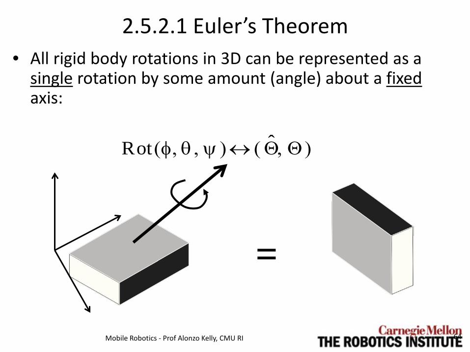
2.5.2.1 Euler’s Theorem • All rigid body rotations in 3D can be represented as a
single rotation by some amount (angle) about a fixed axis:
=
Rot φ θ ψ, ,( ) Θ Θ,( )↔

65 Mobile Robotics - Prof Alonzo Kelly, CMU RI
2.5.2.2 Rotation Vector Representation
• Idea: Use a unit vector scaled by the magnitude of the rotation:
• The axis of rotation is:
• This is not a true vector in the
linear algebra sense. – Cannot be added vectorially to
produce a meaningful result.
Θ Θ Θ⁄=
Θ θx θy θz
T=

66 Mobile Robotics - Prof Alonzo Kelly, CMU RI
2.5.2.3 Relationship to Angular Velocity
• Suppose the rotation angle is differentially small.
• The angular velocity is such that:
• This is a true vector in the linear algebra sense.
• Conversely, the rotation vector is:
dΘ dθx dθy dθzT
=
dΘ ω dt ωx ωy ωz
Tdt= =
ω dΘdt
---------- dΘdΘ
---------- ωdΘ ωω = = =
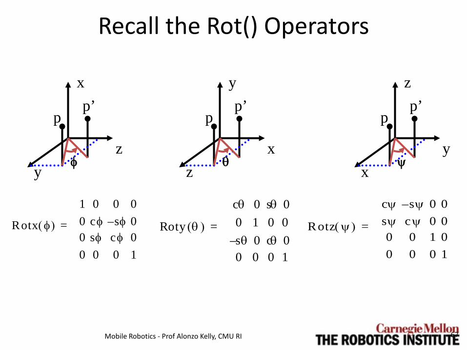
Recall the Rot() Operators
67 Mobile Robotics - Prof Alonzo Kelly, CMU RI
Rotz ψ( )
cψ s– ψ 0 0sψ cψ 0 00 0 1 00 0 0 1
=
z
x y
ψ
p p’
y
z x
θ
p p’
x
y z
φ
p p’
Roty θ( )
cθ 0 sθ 00 1 0 0s– θ 0 cθ 00 0 0 1
=Rotx φ( )
1 0 0 00 cφ sφ– 00 sφ cφ 00 0 0 1
=
68 Mobile Robotics - Prof Alonzo Kelly, CMU RI
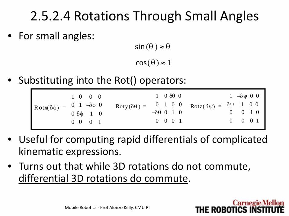
2.5.2.4 Rotations Through Small Angles • For small angles:
• Substituting into the Rot() operators:
• Useful for computing rapid differentials of complicated kinematic expressions.
• Turns out that while 3D rotations do not commute, differential 3D rotations do commute.
θ( )sin θ≈
θ( )cos 1≈
Rotz δψ( )
1 δψ– 0 0δψ 1 0 00 0 1 00 0 0 1
=Rotx δφ( )
1 0 0 00 1 δφ– 00 δφ 1 00 0 0 1
= Roty δθ( )
1 0 δθ 00 1 0 0δθ– 0 1 00 0 0 1
=

69 Mobile Robotics - Prof Alonzo Kelly, CMU RI
General Differential Rotations • Consider a 3D composite differential rotation:
• Substituting into the differential Rot() operators and cancelling H.O.T:
• To first order, the result does not depend on the order the rotations are applied.
δΘ δφ δθ δψT
=
Rotx δφ( )Roty δθ( )Rotz δψ( ) Rot δΘ( )
1 δψ– δθ 0δψ 1 δφ– 0δθ– δφ 1 00 0 0 1
= =

70 Mobile Robotics - Prof Alonzo Kelly, CMU RI
2.5.2.4 Skew Matrices • Last result can be written in terms of a skew matrix:
• Where:
Rot δΘ( ) I δΘ[ ]+ X=
Beware: TYPO in book! This is correct

Outline • 2.4 Kinematics of Mechanisms • 2.5 Orientation and Angular Velocity
– 2.5.1 Orientation in Euler Angle Form – 2.5.2 Angular Rates and Small Angles – 2.5.3 Angular Velocity and Orientation Rates in Euler
Angle Form – 2.5.4 Angular Velocity and Orientation Rates in Angle-
Axis Form – 2.5.5 Summary
Mobile Robotics - Prof Alonzo Kelly, CMU RI 71

72 Mobile Robotics - Prof Alonzo Kelly, CMU RI
2.5.3.1 Relation to Euler Angle rates • The pitch θ, yaw ψ, and roll φ angles are
called Euler angles. • Their rates are not exactly the angular
velocity vector. ω
ωx
ωy
ωz
=
x y
z
tdd
θφψ
measured about moving axes
measured about fixed axes

73 Mobile Robotics - Prof Alonzo Kelly, CMU RI
Relation to Euler Angle rates • Use Chain Rule. Convert coordinates for
each component into the body frame. Note use of transform matrices (from world to body).
x y
z
“unrolled” “unpitched”
“unrolled”
Why express ω in the body frame?
ωbφ·
0·
0
rot x φ,( )0
θ·
0
rot x φ,( ) rot y θ,( )00ψ·
+ +=
ωbωx
ωy
ωz
φ· sθψ·–
cφθ· sφcθψ·+
sφ θ·– cφcθψ·+
1 0 sθ–0 cφ s φcθ0 sφ– cφcθ
φ·
θ·
ψ·
= = =
Note Lowercase “r” in rot

74 Mobile Robotics - Prof Alonzo Kelly, CMU RI
Inverted form • Most useful in inverted form:
• because: • because:
x y
z
Why convert ω to Euler Angle Rates?
φ·
θ·
ψ·
ωx ωysφtθ ωzcφtθ+ +
ωycφ ωzsφ–
ωysφcθ------ ωz
cφcθ------+
1 sφ tθ cφ tθ0 cφ sφ–
0 sφcθ------ cφ
cθ------
ωx
ωy
ωz
= =
ωzcφ ωysφ+ cθψ·=
ωycφ ωzsφ– θ·=

Outline • 2.4 Kinematics of Mechanisms • 2.5 Orientation and Angular Velocity
– 2.5.1 Orientation in Euler Angle Form – 2.5.2 Angular Rates and Small Angles – 2.5.3 Angular Velocity and Orientation Rates in Euler
Angle Form – 2.5.4 Angular Velocity and Orientation Rates in Angle-
Axis Form – 2.5.5 Summary
Mobile Robotics - Prof Alonzo Kelly, CMU RI 75

76 Mobile Robotics - Prof Alonzo Kelly, CMU RI
2.5.4.1 Angular Velocity as a Skew Matrix
• Recall the skew matrix formed from such a small 3D rotation.
• Dividing by dt permits an equivalent matrix to be formed from the angular velocity vector:
Skew dΘ( ) dΘ[ ]X
0 dθz– dθy 0
dθz 0 dθx– 0dθy– dθx 0 0
0 0 0 0
= =
Ω Skew dΘdt-------
ω[ ]X
0 ωz– ωy 0
ωz 0 ωx– 0ωy– ωx 0 0
0 0 0 0
= = =
This is very closely related to the derivative of a rotation matrix.

77 Mobile Robotics - Prof Alonzo Kelly, CMU RI
2.5.4.2 Time Derivative of a Rotation Matrix • Let the matrix track the orientation of a
moving frame k with respect to frame n. • For small time steps, the update to time k+1
is a composition with a small perturbation:
• By definition of derivative:
n
k
k+1
nkR
Rk 1+n Rk
nRk 1+k Rk
n I δΘ[ ]+ X [ ]= =
R·
kn δRk
n
δ t---------
δt 0→lim
Rkn t δ t+( ) Rk
n t( )–[ ]δt
------------------------------------------------δt 0→lim= =

78 Mobile Robotics - Prof Alonzo Kelly, CMU RI
2.5.4.2 Time Derivative of a Rotation Matrix • Recall from last slide:
• Write this in terms of a perturbation.
• Hence, since is fixed:
• Hence:
n
k
k+1
R·
kn δRk
n
δ t---------
δt 0→lim
Rkn t δ t+( ) Rk
n t( )–[ ]δt
------------------------------------------------δt 0→lim= =
R·
kn Rk
n I δΘ[ ]+ X [ ] Rkn–[ ]
δt------------------------------------------------------------
δt 0→lim=
R·
kn Rk
n δΘ[ ]X
δ t----------------------
δt 0→lim Rk
n δΘ[ ]X
δt----------------
δt 0→lim= =
nkR
R·
kn
Rkn
tdd Θ[ ]X
RknΩk= =
79 Mobile Robotics - Prof Alonzo Kelly, CMU RI
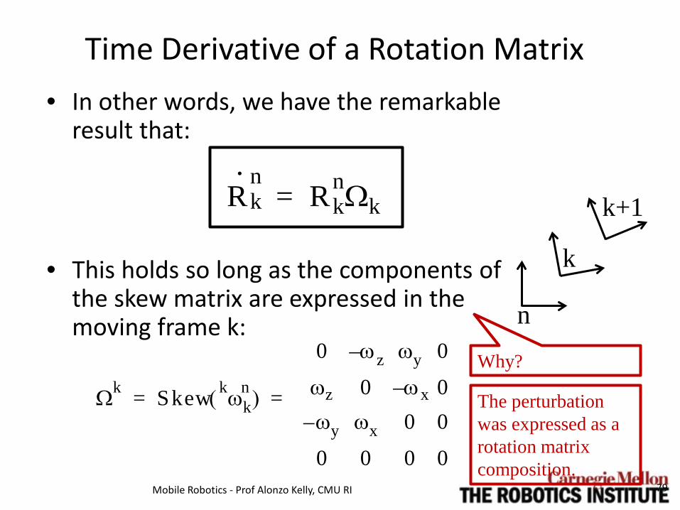
Time Derivative of a Rotation Matrix • In other words, we have the remarkable
result that:
• This holds so long as the components of
the skew matrix are expressed in the moving frame k:
n
k
k+1 R·
kn
RknΩk=
Ωk Skew ωk nk( )
0 ωz– ωy 0
ωz 0 ωx– 0ωy– ωx 0 0
0 0 0 0
= =
Why?
The perturbation was expressed as a rotation matrix composition.

80 Mobile Robotics - Prof Alonzo Kelly, CMU RI
2.5.4.3 Direction Cosines from Angular Velocity • Once again, compound the angular
perturbations thus:
• Based on previous derivative formula:
• Assuming the integrand is constant over a small time step, we have:
Rk 1+n Rk
nRk 1+k=
Rk 1+n Rk
n dΘ[ ]X exp=
Rk 1+k Ωk τd
tk
tk 1+
∫=
A τd0
t
∫ At exp=
Recall:

81 Mobile Robotics - Prof Alonzo Kelly, CMU RI
Direction Cosines from Angular Velocity • This can be written in terms of two
simple functions because for any v:
• But its easy to show that:
• Etc. So, this simplifies to:
v[ ]X exp I v[ ]X v[ ]X( )2
2!------------------
v[ ]X( )3
3!------------------
v[ ]X( )4
4!------------------ …+ + + + +=
vX exp I f1 v( ) v[ ]X f2 v( ) v[ ]X( )2
+ +=
f1 v( ) vsinv
----------= f2 v( ) 1 vcos–( )
v2-------------------------=
v[ ]X[ ]3
v2 vX–= v[ ]X[ ]4
v2 vX[ ]2
–=
82 Mobile Robotics - Prof Alonzo Kelly, CMU RI
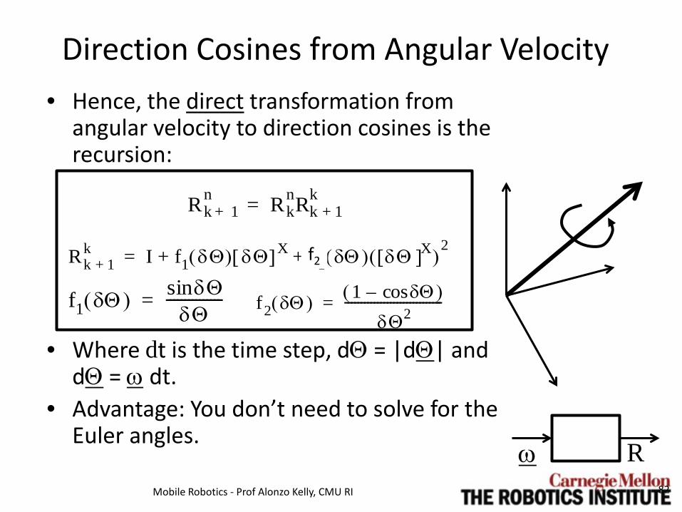
Direction Cosines from Angular Velocity • Hence, the direct transformation from
angular velocity to direction cosines is the recursion:
• Where dt is the time step, dΘ = |dΘ| and dΘ = ω dt.
• Advantage: You don’t need to solve for the Euler angles.
Rk 1+n Rk
nRk 1+k=
f1 δΘ( ) δΘsinδΘ
---------------= f2 δΘ( ) 1 δΘcos–( )
δΘ2------------------------------=
ω R
Rk 1+k I f1 δΘ( ) δΘ[ ]X f1 δΘ( ) δΘ[ ]X( )
2+ += f2

Outline • 2.4 Kinematics of Mechanisms • 2.5 Orientation and Angular Velocity
– 2.5.1 Orientation in Euler Angle Form – 2.5.2 Angular Rates and Small Angles – 2.5.3 Angular Velocity and Orientation Rates in Euler
Angle Form – 2.5.4 Angular Velocity and Orientation Rates in Angle-
Axis Form – 2.5.5 Summary
Mobile Robotics - Prof Alonzo Kelly, CMU RI 83

84 Mobile Robotics - Prof Alonzo Kelly, CMU RI
Summary
• The RPY matrix is yet another compound orthogonal operator matrix. Unlike the DH matrix, it has 6 dof, so it is completely general.
• Angular velocity is the time derivative of the rotation vector.
• Compositions of small angle rotations behave commutatively.
• Angular velocity and small rotations can be expressed as skew matrices.
• Angular velocity is related in a complicated manner to the rates of roll, pitch, and yaw angles.
• The skew of angular velocity is related in a more elegant manner to the rate of the rotation matrix.


