CHAPTER 23 METEOROLOGICAL RADAR Robert J. Serafin National Center for Atmospheric Research* 23.1 INTRODUCTION As this handbook is being written, dramatic changes are taking place in the field of radar meteorology. While the majority of radar engineers are familiar withcur- rent operational meteorological radars, few are aware of the advances that have been made in the past two decades. For example, doppler radar meteorology, us- ing modern digital signal-processing techniques and display technology, has moved ahead so rapidly that the United States is now planning to replace its ex- isting operational weather radar network with a next-generation doppler system (NEXRAD). This system will provide quantitative and automated real-time infor- mation on storms, precipitation, hurricanes, tornadoes, and a host of other im- portant weather phenomena, with higher spatial and temporal resolution than ever before. 1 A second network of doppler radars, in airport terminal areas, will provide quantitative measurements of gust fronts, wind shear, microbursts, and other weather hazards for improving the safety of operations at major airports in the United States. 1 ' 2 Next-generation doppler radars that use flat-plate antennas, color displays, and solid-state transmitters are now available for commercial air- craft. And many of these new technologies are being deployed in countries throughout the world. In the research arenas, multiple-doppler radars are used for deriving three- dimensional wind fields. 3 Airborne doppler radar 4 ' 5 has been used to duplicate these capabilities, thus providing for great mobility. Polarization diversity techniques 6 are used for discriminating ice particles from water, for improved quantitative precipitation measurement, and for detecting hail. And there is a new family of radars, ultrahigh-frequency (UHF) and very-high-frequency (VHF) fixed-beam systems that are being used to obtain continuous profiles of horizon- tal winds. 7 These examples are illustrative of the vitality of the field. This chapter is intended to introduce the reader to meteorological radar and particularly those system characteristics that are unique to meteorological appli- cations. In this regard, it should be noted that most meteorological radars appear *The National Center for Atmospheric Research is sponsored by the National Science Foundation. Special thanks are due to Victoria Holzhauer for her careful typing, assistance with figures, and ed- iting of this manuscript. The author is also grateful to Richard Carbone and Jeffrey Keeler for their crit- ical reviews.
Transcript
CHAPTER 23METEOROLOGICAL RADAR
Robert J. SerafinNational Center for Atmospheric Research*
23.1 INTRODUCTION
As this handbook is being written, dramatic changes are taking place in the fieldof radar meteorology. While the majority of radar engineers are familiar with cur-rent operational meteorological radars, few are aware of the advances that havebeen made in the past two decades. For example, doppler radar meteorology, us-ing modern digital signal-processing techniques and display technology, hasmoved ahead so rapidly that the United States is now planning to replace its ex-isting operational weather radar network with a next-generation doppler system(NEXRAD). This system will provide quantitative and automated real-time infor-mation on storms, precipitation, hurricanes, tornadoes, and a host of other im-portant weather phenomena, with higher spatial and temporal resolution thanever before.1 A second network of doppler radars, in airport terminal areas, willprovide quantitative measurements of gust fronts, wind shear, microbursts, andother weather hazards for improving the safety of operations at major airports inthe United States.1'2 Next-generation doppler radars that use flat-plate antennas,color displays, and solid-state transmitters are now available for commercial air-craft. And many of these new technologies are being deployed in countriesthroughout the world.
In the research arenas, multiple-doppler radars are used for deriving three-dimensional wind fields.3 Airborne doppler radar4'5 has been used to duplicatethese capabilities, thus providing for great mobility. Polarization diversitytechniques6 are used for discriminating ice particles from water, for improvedquantitative precipitation measurement, and for detecting hail. And there is anew family of radars, ultrahigh-frequency (UHF) and very-high-frequency (VHF)fixed-beam systems that are being used to obtain continuous profiles of horizon-tal winds.7 These examples are illustrative of the vitality of the field.
This chapter is intended to introduce the reader to meteorological radar andparticularly those system characteristics that are unique to meteorological appli-cations. In this regard, it should be noted that most meteorological radars appear
*The National Center for Atmospheric Research is sponsored by the National Science Foundation.Special thanks are due to Victoria Holzhauer for her careful typing, assistance with figures, and ed-
iting of this manuscript. The author is also grateful to Richard Carbone and Jeffrey Keeler for their crit-ical reviews.
similar to radars used for other purposes. Pulsed and pulsed doppler systems arecommon. Parabolic dish antennas, focal-point feeds, and low-noise solid-state re-ceivers are used. Magnetrons, phase-locked magnetrons, klystrons, traveling-wave tubes, and other forms of transmitters are used.
The major distinction between meteorological radar and other kinds of radarslies in the nature of the targets. Meteorological targets are distributed in spaceand occupy a large fraction of the spatial resolution cells observed by the radar.Moreover, it is necessary to make quantitative measurements of the received sig-nal's characteristics in order to estimate such parameters as precipitation rate,precipitation type, air motion, turbulence, and wind shear. In addition, becauseso many radar resolution cells contain useful information, meteorological radarsrequire high-data-rate recording systems and effective means for real-timedisplay.8'9 Thus, while many radar applications call for discrimination of a rela-tively few targets from a clutter background, meteorological radars focus on mak-ing accurate estimates of the nature of the weather clutter itself. This poses somechallenging problems for the radar system designer to address.
The discussion here will refer to a number of useful texts and references forthe reader to use. However, Battan's text,10 revised in 1973, deserves specialmention for its clarity and completeness and remains a standard for courses inradar meteorology that are taught in universities around the world. Doviak andZrnic11 place special emphasis on doppler meteorological radar. Chapter 24 in thefirst "Radar Handbook," by Bean et al.,12 addresses the problem of weather ef-fects on radar. Finally, perhaps the broadest and most complete set of referenceson progress in the field can be found in the Proceedings and Preprints of the se-ries of radar meteorology conferences sponsored by the American Meteorologi-cal Society (AMS). These documents can be found in most technical libraries andalso can be obtained through the offices of the AMS in Boston.
23.2 THE RADAR RANGE EQUATION FORMETEOROLOGICAL TARGETS
The received power from distributed targets can be derived from any of a varietyof expressions that are applicable to radar in general. A simple form, with whichto begin, is given below:
Pr = ̂ (23.1)
where (3 is a constant dependent upon radar system parameters, r is the range,and a is the radar cross section.
It is in the calculation of a for meteorological targets that the radar range equa-tion differs from that for point targets, cr may be written
<j = T]V (23.2)
where r\ is the radar reflectivity in units of cross-sectional area per unit volumeand V is the volume sampled by the radar. T) can be written as
N
TI = ]>>, (23.3)/=i
where N is the number of scatterers per unit volume and (J1 is the backscatteringcross section of the ith scatterer. In general, the meteorological scatterers cantake on a variety of forms, which include water droplets, ice crystals, hail, snow,and mixtures of the above.
Mie13 developed a general theory for the energy backscattered by a planewave impinging on spherical drops. This backscattered energy is a function of thewavelength, the complex index of refraction of the particle, and the ratio 2ira/X,where a is the radius of the spherical particle and X is the wavelength.
When the ratio 2ira/X — 1, the Rayleigh approximation10 may be applied, andcr, becomes
CT1- = ^IATI2A6 (23.4)X
where D1 is the diameter of the /th drop and
™2 i 2\K\2= ^-^ (23.5)
m2 + 2
where m is the complex index of refraction. At temperatures between O and 2O0C,for the water phase, and at centimeter wavelengths
\K\2 * 0.93 (23.60)
and for the ice phase
\K\2 * 0.20 (23.66)
Equation (23.3) can now be written as
5 NTI = 5JlJTI2^X (23.7)
X 1=1
and the radar reflectivity factor Z defined as
N
Z ]?A6 (23.8)/=i
In radar meteorology, it is common to use the dimensions of millimeters fordrop diameters D1 and to consider the summation to take place over a unit vol-ume of size 1 m3. Therefore, the conventional unit of Z is in mm6/m3. For iceparticles, D1 is given by the diameter of the water droplet that would result if theice particle were to melt completely.
It is often convenient to treat the drop or particle size distribution as a con-tinuous function with a number density N(D), where N(D) is the number of dropsper unit volume, with diameters between D and D + dD. In this case, Z is givenby the sixth moment of the particle size distribution,
Z = r N(D)D6JD (23.9)%/ o
If the radar beam is filled with scatterers, the sample volume V is given10 ap-proximately by
v _ 2^fn (231Q)
8where 9 and <(> are the azimuth and elevation beamwidths, c is the velocity oflight, and T is the radar pulsewidth.
Substituting Eqs. (23.10), (23.2), and (23.4) into Eq. (23.1) gives
P, = &^$M2Iff
= P2M£IL^Z
8\V
= p/Z
r2
This simple expression illustrates that the received power is a function only of 0'(a constant dependent upon radar system parameters), is proportional to the ra-dar reflectivity factor Z, and is inversely proportional to r.
In actual fact, the antenna gain is not uniform over the beam width, and theassumption of a uniform gain can lead to errors in the calculation of Z. Probert-Jones14 took this into account, assumed a gaussian shape for the antenna beam,and derived the following equation for the received power:
P,G2X2e<|>CT "Pr = ^ 2X <23'12)512(2 In Z)TT2T2 £1
where 2 In 2 is the correction due to the gaussian-shaped beam.By using the relationships in Eqs. (23.7) and (23.8), Eq. (23.12) can be written
in terms of the reflectivity factor Z as
Pfj2*$crti*\K\2ZPr = I-T- (23.13)
512(2 In 2)rV
One must be careful to use consistent units in Eq. (23.13). If meter-kilogram-seconds (mks) units are used, the calculation of Z from Eq. (23.13) will have di-mensions of m6/m3. Conversion to the more commonly used units of mm6/m3 re-quires that the result be multiplied by the factor 1018. Because Z values of interestcan range over several orders of magnitude, a logarithmic scale is often used,where
dBZ = 10 log Z (23.14)Equation (23.13) can be used to measure the reflectivity factor Z when the an-
tenna beam is filled, when the Rayleigh approximation is valid, and when thescatterers are in either the ice or the water phase. Because all these conditions
are not always satisfied, it is common to use the term Z6, the effective reflectivityfactor, in place of Z. When Ze is used, it is generally understood that the aboveconditions are assumed. Practitioners in the field of radar meteorology often useZe and Z interchangeably, albeit incorrectly.
Finally, it is important to note the range of Z values that are of meteorologicalsignificance. In nonprecipitating clouds, Z values as small as —40 dBZ are of in-terest. In the optically clear boundary layer, Z values of the order -20 dBZ to 10dBZ are of interest. In rain, Z may range from about 20 dBZ to as much as 60dBZ, with a 55 to 60 dBZ rain being of the type that can cause severe flooding.Severe hailstorms may produce Z values higher than 70 dBZ. Operational radarsare generally designed to detect Z values ranging from 10 to 60 dBZ, while re-search applications usually aim for the maximum dynamic range possible. In lightof the above, operational radars often employ sensitivity time control (STC) tocompensate for inverse r2 dependence, but research radars usually do not useSTC owing to the attendant loss of sensitivity at short ranges.
23.3 DESIGNCONSIDERATIONS
Three of the more significant factors that affect the design of meteorological ra-dars are attenuation, range-velocity ambiguities, and ground clutter. The combi-nation of these three, along with the need to obtain adequate spatial resolution,leads to a wavelength selection in the range of 3 to 10 cm for most meteorologicalapplications.
Attenuation Effects. Attenuation has at least two negative effects onmeteorological radar signals. First, because of attenuation it becomes difficult,if not impossible, to make quantitative measurements of the backscatteredenergy from precipitation which is at greater range (and at the same azimuthand elevation angles) than precipitation closer to the radar. This inability toprecisely measure the backscattering cross section makes quantitativemeasurements of precipitation rates more difficult.
Second, if the attenuation due to precipitation or the intervening medium issufficiently great, the signal from a precipitation cell behind a region of strongabsorption may be totally obliterated, leading to potentially disastrous effects.One example of the potentially serious consequences of very strong absorption isthe impact it might have on airborne storm avoidance radars, most of which arein the 3-cm band, although some use a 5-cm wavelength. Metcalf15 has examinedground-based radar data from the storm that was responsible for the 1977 crash ofSouthern Airways Flight 242 in northwest Georgia. The crew had relied on itson-board radar for penetration of a severe storm. Metcalf shows strong evidencethat the region penetrated by the aircraft, while appearing to be free of echo, hadactually been obliterated because of severe attenuation. Severe storms can alsoproduce very strong absorption at 5-cm wavelength, as noted by Allen et al.16
In some meteorological radar applications, it is desirable to attempt to mea-sure attenuation along selected propagation paths. This is done because absorp-tion is related to liquid-water content and can provide useful information for thedetection of such phenomena as hail, in accordance with the dual-wavelengthtechnique described by Eccles and Atlas.17
In the following subsections, quantitative expressions relating attenuation toprecipitation are given. Much of this is taken from Bean, Button, and Warner.12
Rattan's textbook10 is also an excellent source for additional information on theabsorbing properties of precipitation.
Attenuation in Clouds. Cloud droplets are regarded here as those water orice particles having radii smaller than 100 jxm, or 0.01 cm. For wavelengths ofincident radiation well in excess of 0.5 cm, the attenuation becomes independentof the drop-size distribution. The generally accepted equations for attenuation byclouds usually show the moisture component of the equations in the form of theliquid-water content (grams per cubic meter). Observations indicate that theliquid-water concentration in clouds generally ranges from18 1 to 2.5 g/m3, al-though Weickmann and aufm Kampe19 have reported isolated instances of cumu-lus congestus clouds with water contents of 4.0 g/m3 in the upper levels. In iceclouds, it rarely exceeds 0.5 and is often less than 0.1 g/m3. The attenuation dueto cloud drops may be written12
K = K1M (23.15)
where K = attenuation, dB/kmK1 = attenuation coefficient, dB/(km • g • m3)M = liquid-water content, g/m3
M = ̂ iX (23.16)3 /=i
K1 = 0.4343^Im(- ̂ r^} (23.17)x \ m2 + 2/
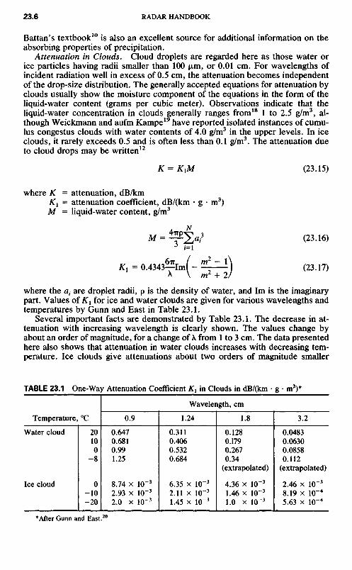
where the at are droplet radii, p is the density of water, and Im is the imaginarypart. Values of K1 for ice and water clouds are given for various wavelengths andtemperatures by Gunn and East in Table 23.1.
Several important facts are demonstrated by Table 23.1. The decrease in at-tenuation with increasing wavelength is clearly shown. The values change byabout an order of magnitude, for a change of A. from 1 to 3 cm. The data presentedhere also shows that attenuation in water clouds increases with decreasing tem-perature. Ice clouds give attenuations about two orders of magnitude smaller
TABLE 23.1 One-Way Attenuation Coefficient ^1 in Clouds in dB/(km • g • m3)*
*After Gunn and East.20
Temperature, 0C
Water cloud
Ice cloud
2010
O-8
O-10-20
0.9
0.6470.6810.991.25
8.74 x 10~3
2.93 x 1(T3
2.0 x 1(T3
Wavelength, cm
1.24
0.3110.4060.5320.684
6.35 x 1(T3
2.11 x 10~3
1.45 x 1(T3
1.8
0.1280.1790.2670.34
(extrapolated)
4.36 x 1(T3
1.46 x 10"3
1.0 x lO"3
3.2
0.04830.06300.08580.112
(extrapolated)
2.46 x 10~3
8.19 x 10~4
5.63 x 1(T4
than water clouds of the same water content. The attenuation of microwaves byice clouds can be neglected for all practical purposes.10
Attenuation by Rain. Ryde and Ryde21 calculated the effects of rain on mi-crowave propagation and showed that absorption and scattering effects of rain-drops become more pronounced at the higher microwave frequencies, where thewavelength and the raindrop diameters are more nearly comparable. In the 10-cmband and at shorter wavelengths the effects are appreciable, but at wavelengthsin excess of 10 cm the effects are greatly decreased. It is also known that sus-pended water droplets and rain have an absorption rate in excess of that of thecombined oxygen and water-vapor absorption.22
In practice, it has been convenient to express rain attenuation as a function ofthe precipitation rate R, which depends on both the liquid-water content and thefall velocity of the drops, the latter in turn depending on the size of the drops.
Ryde23 studied the attenuation of microwaves by rain and deduced, by usingLaws and Parsons24 distributions, that this attenuation in decibels per kilometercan be approximated by
KR = J^r° [R(r)Tdr (23.18)
where KR = total attenuation, dBK = function of frequency25
R(r) = rainfall rate along path rr0 = length of propagation path, kma = function of frequency10
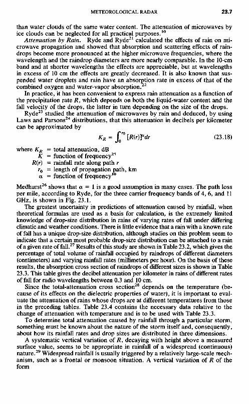
Medhurst26 shows that a = 1 is a good assumption in many cases. The path lossper mile, according to Ryde, for the three carrier frequency bands of 4, 6, and 11GHz, is shown in Fig. 23.1.
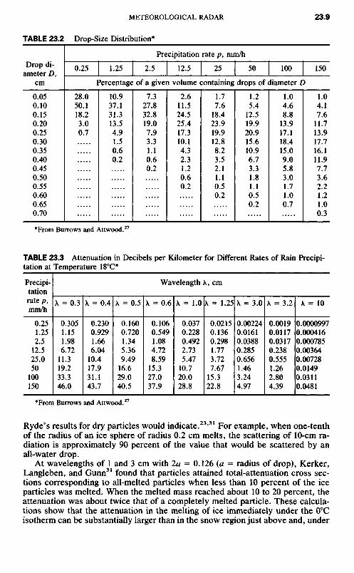
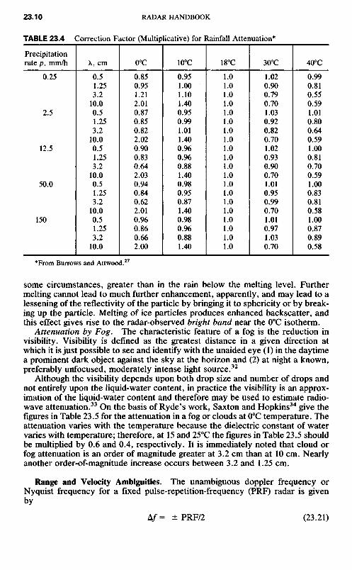
The greatest uncertainty in predictions of attenuation caused by rainfall, whentheoretical formulas are used as a basis for calculation, is the extremely limitedknowledge of drop-size distribution in rains of varying rates of fall under differingclimatic and weather conditions. There is little evidence that a rain with a known rateof fall has a unique drop-size distribution, although studies on this problem seem toindicate that a certain most probable drop-size distribution can be attached to a rainof a given rate of fall.27 Results of this study are shown in Table 23.2, which gives thepercentage of total volume of rainfall occupied by raindrops of different diameters(centimeters) and varying rainfall rates (millimeters per hour). On the basis of theseresults, the absorption cross section of raindrops of different sizes is shown in Table23.3. This table gives the decibel attenuation per kilometer in rains of different ratesof fall for radio wavelengths between 0.3 and 10 cm.
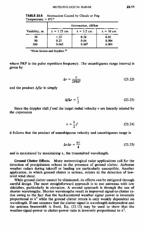
Since the total-attenuation cross section28 depends on the temperature (be-cause of its effects on the dielectric properties of water), it is important to eval-uate the attenuation of rains whose drops are at different temperatures from thosein the preceding tables. Table 23.4 contains the necessary data relative to thechange of attenuation with temperature and is to be used with Table 23.3.
To determine total attenuation caused by rainfall through a particular storm,something must be known about the nature of the storm itself and, consequently,about how its rainfall rates and drop sizes are distributed in three dimensions.
A systematic vertical variation of R, decaying with height above a measuredsurface value, seems to be appropriate in rainfall of a widespread (continuous)nature.29 Widespread rainfall is usually triggered by a relatively large-scale mech-anism, such as a frontal or monsoon situation. A vertical variation of R of theform
R A I N F A L L RATE (in/h)
FIG. 23.1 Theoretical rain attenuation versus rainfall rate.
R = RQe~dh2 (23.19)
can be assumed to be appropriate under continuous-rainfall conditions.29 In Eq.(23.19), R0 is the surface rainfall rate, h is the height above the earth's surface,and d is a constant, equal to about 0.2.
Convective-type precipitation, however, shows a quite different nature. Thepresence of the virga (precipitation aloft but evaporating before reaching the sur-face) associated with so many shower-type clouds indicates that Eq. (23.19) is notespecially representative of shower rainfall. Dennis30 has done considerable workin examining rainfall determinations in shower-type activity. His observationsshow that the reflectivity factor Z(mm6/m3) of an element of a vertical slice takenthrough a spherical shower cell is well represented by a regression line of theform
Z = Cl(ro - r)c2 (23.20)
In Eq. (23.20), r is the distance from the center of the cell of radius r0, and C1 andC2 are positive constants.
Attenuation by Hail. Ryde23 concluded that the attenuation caused by hail isone-hundredth of that caused by rain, that ice-crystal clouds cause no sensibleattenuation, and that snow produces very small attenuation even at the excessiverate of fall of 5 in/h. However, the scattering by spheres surrounded by a con-centric film of different dielectric constant does not give the same effect that
EXCE
SS P
ATH
LOSS
(dB/
mi)
*From Burrows and Attwood.27
Ryde's results for dry particles would indicate.23'31 For example, when one-tenthof the radius of an ice sphere of radius 0.2 cm melts, the scattering of 10-cm ra-diation is approximately 90 percent of the value that would be scattered by anall-water drop.
At wavelengths of 1 and 3 cm with 2a = 0.126 (a = radius of drop), Kerker,Langleben, and Gunn31 found that particles attained total-attenuation cross sec-tions corresponding to all-melted particles when less than 10 percent of the iceparticles was melted. When the melted mass reached about 10 to 20 percent, theattenuation was about twice that of a completely melted particle. These calcula-tions show that the attenuation in the melting of ice immediately under the O0Cisotherm can be substantially larger than in the snow region just above and, under
some circumstances, greater than in the rain below the melting level. Furthermelting cannot lead to much further enhancement, apparently, and may lead to alessening of the reflectivity of the particle by bringing it to sphericity or by break-ing up the particle. Melting of ice particles produces enhanced backscatter, andthis effect gives rise to the radar-observed bright band near the O0C isotherm.
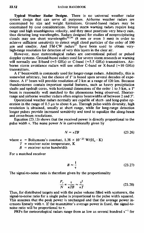
Attenuation by Fog. The characteristic feature of a fog is the reduction invisibility. Visibility is defined as the greatest distance in a given direction atwhich it is just possible to see and identify with the unaided eye (1) in the daytimea prominent dark object against the sky at the horizon and (2) at night a known,preferably unfocused, moderately intense light source.32
Although the visibility depends upon both drop size and number of drops andnot entirely upon the liquid-water content, in practice the visibility is an approx-imation of the liquid-water content and therefore may be used to estimate radio-wave attenuation.33 On the basis of Ryde's work, Saxton and Hopkins34 give thefigures in Table 23.5 for the attenuation in a fog or clouds at O0C temperature. Theattenuation varies with the temperature because the dielectric constant of watervaries with temperature; therefore, at 15 and 250C the figures in Table 23.5 shouldbe multiplied by 0.6 and 0.4, respectively. It is immediately noted that cloud orfog attenuation is an order of magnitude greater at 3.2 cm than at 10 cm. Nearlyanother order-of-magnitude increase occurs between 3.2 and 1.25 cm.
Range and Velocity Ambiguities. The unambiguous doppler frequency orNyquist frequency for a fixed pulse-repetition-frequency (PRF) radar is givenby
A/= ± PRF/2 (23.21)
TABLE 23.4 Correction Factor (Multiplicative) for Rainfall Attenuation*
where PRF is the pulse repetition frequency. The unambiguous range interval isgiven by
A^ = 2^F (23'22)
and the product A/Ar is simply
A/Ar = ^ (23.23)
Since the doppler shift/and the target radial velocity v are linearly related bythe expression
v = I/ (23.24)
it follows that the product of unambiguous velocity and unambiguous range is
AvAr = ̂ (23.25)4
and is maximized by maximizing X, the transmitted wavelength.
Ground Clutter Effects. Many meteorological radar applications call for thedetection of precipitation echoes in the presence of ground clutter. Airborneweather radars during takeoff or landing are particularly susceptible. Anotherapplication, in which ground clutter is serious, relates to the detection of low-level wind shear.
While ground clutter cannot be eliminated, its effects can be mitigated throughcareful design. The most straightforward approach is to use antennas with lowsidelobes, particularly in elevation. A second approach is through the use ofshorter wavelengths. Shorter wavelengths result in improved signal-to-clutter ra-tios owing to the fact that the backscattered weather signal power is inverselyproportional to X4 while the ground clutter return is only weakly dependent onwavelength. If one assumes that the clutter signal is wavelength-independent andthe antenna beamwidth is fixed, Eq. (23.13) may be used to show that theweather-signal-power to clutter-power ratio is inversely proportional to X2.
TABLE 23.5 Attenuation Caused by Clouds or FogTemperature = O0C*
Visibility, m
3090
300
Attenuation, dB/km
X = 1.25 cm
1.250.250.045
X = 3.2 cm
0.200.040.007
X = 10 cm
0.020.0040.001
Typical Weather Radar Designs. There is no universal weather radarsystem design that can serve all purposes. Airborne weather radars areconstrained by size and weight limitations. Ground-based radars may beconstrained by cost considerations. Severe storm warning radars require longrange and high unambiguous velocity, and they must penetrate very heavy rain,thus dictating long wavelengths. Radars designed for studies of nonprecipitatingclouds may use short wavelengths35'36 (8 mm or even 3 mm) in order toachieve sufficient sensitivity to detect small cloud particles of the order of 100|xm and smaller. And FM-CW radars37 have been used to obtain very-high-range resolution for detection of very thin layers in the clear air.
However, most meteorological radars are conventional pulsed or pulseddoppler systems. Ground-based radars used for severe storm research or warningwill normally use S-band («3 GHz) or C-band («5.5 GHz) transmitters. Air-borne storm avoidance radars will use either C-band or X-band («10 GHz)transmitters.
A l 0 beam width is commonly used for longer-range radars. Admittedly, this issomewhat arbitrary, but the choice of 1° is based upon several decades of expe-rience. A l 0 beam will provide resolution of 2 km at a range of 120 km. Becausethunderstorms contain important spatial features, such as heavy precipitationshafts and updraft cores, with horizontal dimensions of the order 1 to 5 km, a 1°beam is reasonably well matched to the phenomena being observed. Shorter-range and airborne weather radars often employ beamwidths of between 2 and 3°.
Operational weather radars normally are capable of short- and long-pulse op-eration in the range of 0.5 JJLS to about 6 jxs. Through pulse-width diversity, highresolution is obtained, usually at short range, while for long-range detectionlonger pulses provide increased sensitivity and tend to equalize the along-beamand cross-beam resolutions.
Equation (23.13) shows that the received power is directly proportional to thepulse width T. The noise power N is conventionally given by
N = KTB (23.26)
where K = Boltzmann's constant, 1.38 x 10~23 W/(HZ • K)T = receiver noise temperature, KB = receiver noise bandwidth
For a matched receiver
B « - (23.27)T
The signal-to-noise ratio is therefore given by the proportionality
Pr T T2
Tr a -^ ~ "^ <23'28)N K.TB *T
Thus, for distributed targets and with the pulse volume filled with scatterers, thesignal-to-noise ratio for a single pulse is proportional to the pulse width squared.This assumes that the peak power is unchanged and that the average power in-creases linearly with T. If the transmitter's average power is fixed, the signal-to-noise ratio will be proportional to T.
PRFs for meteorological radars range from as low as several hundred s"1 for
long-range detection to several thousand s l for shorter-wavelength systems at-tempting to achieve high unambiguous velocities. Generally speaking, most me-teorological doppler radars are operated in a single mode, compromising the ra-dar's ability to unambiguously resolve either range or velocity. More recentdesigns, however, may use a dual pulse repetition period38 (PRT) to resolve bothrange and velocity. Another approach39 is to employ a transmitted-pulse se-quence with random phases from pulse to pulse. Range ambiguities cannot be to-tally eliminated, but their effects can be significantly mitigated through these ap-proaches.
To discuss design details of all types of meteorological radars is beyond thescope of this chapter. However, it will be useful to include some of the importantcharacteristics of the NEXRAD radar, which illustrate the performance of a mod-ern operational weather radar ca. 1989. Table 23.6 contains some of the more rel-evant NEXRAD design features.
TABLE 23.6 Some Relevant NEXRAD System Characteristics
23.4 SIGNALPROCESSING
It can be shown8'11 that the received signal from meteorological targets is wellrepresented by a narrowband gaussian process. This is a direct consequence ofthe fact that (1) the number of scatterers in the pulse volume is large (>106); (2)the pulse volume is large compared with the transmitted wavelength; (3) the pulsevolume is filled with scatterers, causing all phases on the range from O to 2ir to bereturned; and (4) the particles are in motion with respect to one another due toturbulence, wind shear, and their varying fall speeds.
The superposition of the scattered electric fields from such a large number ofparticles (each with random phase) gives rise, through the central limit theorem,to a signal with gaussian statistics. Because the particles are in motion with re-spect to one another, there is also a doppler spread, often referred to as the vari-ance of the doppler spectrum. Finally, since all the particles within the samplevolume are moving with some mean or average radial velocity, there is a meanfrequency of the doppler spectrum which is shifted from the transmitted fre-quency.
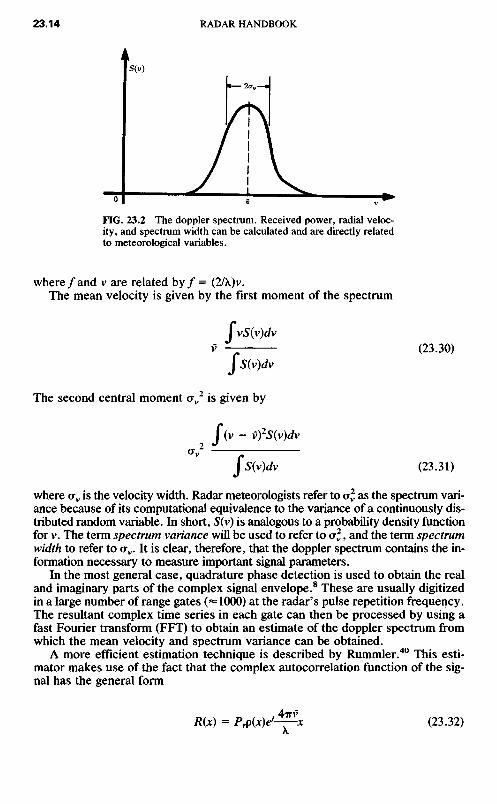
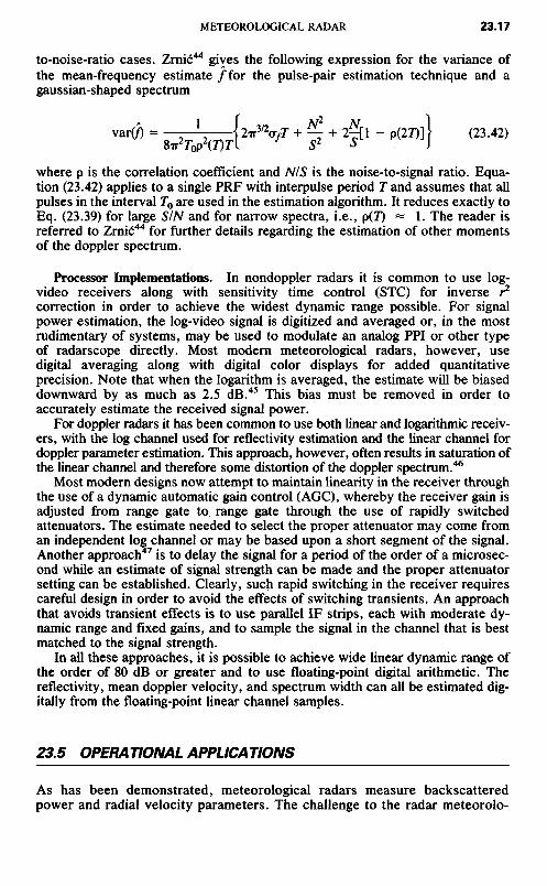
The power spectral density of a meteorological signal is depicted schemati-cally in Fig. 23.2 and can be interpreted as follows. The received power is simplythe integral under the curve and is given by
700,000 W1.6,4.8 JJLS230km±50m/s460km5OdB1°(-8 dBZ at 50 km)
FIG. 23.2 The doppler spectrum. Received power, radial veloc-ity, and spectrum width can be calculated and are directly relatedto meteorological variables.
where/and v are related by/ = (2/X)v.The mean velocity is given by the first moment of the spectrum
fvS(v)dvv — (23.30)
J S(v)dv
The second central moment crv2 is given by
f (v - v)2S(v)dv2 J
"v TJ S(v)dv (23.31)
where av is the velocity width. Radar meteorologists refer to aj as the spectrum vari-ance because of its computational equivalence to the variance of a continuously dis-tributed random variable. In short, 5(v) is analogous to a probability density functionfor v. The term spectrum variance will be used to refer to of, and the term spectrumwidth to refer to av. It is clear, therefore, that the doppler spectrum contains the in-formation necessary to measure important signal parameters.
In the most general case, quadrature phase detection is used to obtain the realand imaginary parts of the complex signal envelope.8 These are usually digitizedin a large number of range gates (—1000) at the radar's pulse repetition frequency.The resultant complex time series in each gate can then be processed by using afast Fourier transform (FFT) to obtain an estimate of the doppler spectrum fromwhich the mean velocity and spectrum variance can be obtained.
A more efficient estimation technique is described by Rummler.40 This esti-mator makes use of the fact that the complex autocorrelation function of the sig-nal has the general form
• 4-TTVR(X) = P^(x)e>^-x (23.32)
A.
where P(JC) is the correlation coefficient and Jt is a dummy variable.It follows that V9 the mean velocity, is given by
v = ̂ arg [R(X)] (23.33)
It can also be shown that
, X2 [ R(x) ]av
2 « -^- 1 -— (23.34)V to?A R(o)-N\
where N is the noise power.This estimator is widely used for mean-frequency estimation with doppler me-
teorological radars. The estimates are unbiased in the presence of noise when thedoppler spectrum is symmetrical. Its greatest appeal, however, is due to its com-putational simplicity. For a pulsed radar, with a pulse repetition period (PRT) T,R(T) is obtained from the simple expression8
(N-I)
*(fl = r;2JJ*+i^ (23.35)yv(*=o)
where the sk are the complex signal samples (sampled at the radar PRT) in a givenrange gate and s*k is the complex conjugate. It is clear that this algorithm requiresonly N complex multiplications for a time series of TV samples while the FFT re-quires N Iog2 N. This pulse-pair algorithm, as it is often called, therefore not onlyis an excellent estimation technique but is less complex and costly than compa-rable FFT processors. In addition, FFT estimates of mean velocity and spectrumwidth are biased by receiver noise. If the FFT approach is used, the bias due tonoise can be removed by estimating the noise threshold in the spectral domainand truncating the derived spectrum.41
For most applications, the pulse-pair processor has become the technique ofchoice. However, in some research applications it remains advantageous to haveaccess to the full doppler spectrum. Very fast and programmable digital signal-processing chips make it possible for radar meteorologists to have their cake andeat it too. Flexibility due to programmability permits tailoring of the processor'scharacteristics to the application from day to day or even beam to beam andrange gate to range gate. Until recently, most pulse-pair or FFT processors formeteorological radars have been hard-wired and therefore inflexible.
Measurement Accuracy. Because the received signals are sample functionsfrom gaussian random processes, the doppler spectrum and its moments cannotbe measured exactly in any finite period of time. Consequently, allmeasurements will be somewhat in error, with the error being a function of theproperties of the atmosphere, the radar wavelength, and the time allocated tothe measurement.
The theoretical development of signal estimator statistics is found inDenenberg, Serafin, and Peach42 for the FFT technique. Doviak and Zrnic11
cover the subject quite completely. Following are some useful expressions for themean square error of mean power and mean velocity estimates.
Power Estimation. It is well known that for a gaussian process,43 usingsquare-law signal detection, samples of the mean power P1. of the process are ex-ponentially distributed with variance P,2. Given a time T0 allocated to the mea-surement and a signal bandwidth Oy(Hz), there will be approximately oy70 inde-pendent samples of the square of the signal envelope. It follows, therefore, thatan estimate P1. of the mean power for this process will have a variance or meansquare error given by
P2
var (Pr] « ̂ - (23.36)OyJ0
Substituting for oy from the expression oy = 2ov/X, where CTV is the width of thedoppler spectrum, Eq. (23.36) becomes
. A/>r2
var (Pr) - -̂ - (23.37)2CT1To
This expression is valid for high signal-to-noise cases.Velocity Estimation. Denenberg, Serafm, and Peach42 give the following ex-
pression for the variance of mean-frequency estimates of the doppler spectrum
var(/) = -J- ff2S2(f + f }df (23.38)P2T0
J
This is an interesting result, showing that the variance of the estimate/is a func-tion only of the shape of the doppler spectrum and the integration time T0. If thespectrum has a gaussian shape, with variance oy2, Eq. (23.38) becomes
var(/) = ^ (23.39)4V^r0
Noting that var(v) = (X/2)2 var (/), we can write
var (v) = —— (23.40)8V^r0
If we multiply numerator and denominator by crv, Eq. (23.40) becomes
Xo-,2 av2
var(v) = — = — (23.41)8VlTCT1To 4 V TTOy-T0
Thus, it is seen that the variance of the mean velocity estimate v is directlyproportional to the variance of the doppler spectrum and inversely proportionalto the number of independent samples. Note also that var (v) is proportional to \,indicating that, for the same processing time T0 and for the same ov, the varianceof the estimate can be reduced by reducing the wavelength, which increases thenumber of independent samples.
Equations (23.38), (23.39), (23.40), and (23.41) are applicable in high signal-
to-noise-ratio cases. Zrnic*44 gives the following expression for the variance ofthe mean-frequency estimate /for the pulse-pair estimation technique and agaussian-shaped spectrum
vartf) - ̂ d^a'T+F+2?" - "'2751I (23-42)
where p is the correlation coefficient and NIS is the noise-to-signal ratio. Equa-tion (23.42) applies to a single PRF with interpulse period T and assumes that allpulses in the interval J0 are used in the estimation algorithm. It reduces exactly toEq. (23.39) for large SIN and for narrow spectra, i.e., p(7) « 1. The reader isreferred to Zrnic44 for further details regarding the estimation of other momentsof the doppler spectrum.
Processor Implementations. In nondoppler radars it is common to use log-video receivers along with sensitivity time control (STC) for inverse r2
correction in order to achieve the widest dynamic range possible. For signalpower estimation, the log-video signal is digitized and averaged or, in the mostrudimentary of systems, may be used to modulate an analog PPI or other typeof radarscope directly. Most modern meteorological radars, however, usedigital averaging along with digital color displays for added quantitativeprecision. Note that when the logarithm is averaged, the estimate will be biaseddownward by as much as 2.5 dB.45 This bias must be removed in order toaccurately estimate the received signal power.
For doppler radars it has been common to use both linear and logarithmic receiv-ers, with the log channel used for reflectivity estimation and the linear channel fordoppler parameter estimation. This approach, however, often results in saturation ofthe linear channel and therefore some distortion of the doppler spectrum.46
Most modern designs now attempt to maintain linearity in the receiver throughthe use of a dynamic automatic gain control (AGC), whereby the receiver gain isadjusted from range gate to range gate through the use of rapidly switchedattenuators. The estimate needed to select the proper attenuator may come froman independent log channel or may be based upon a short segment of the signal.Another approach47 is to delay the signal for a period of the order of a microsec-ond while an estimate of signal strength can be made and the proper attenuatorsetting can be established. Clearly, such rapid switching in the receiver requirescareful design in order to avoid the effects of switching transients. An approachthat avoids transient effects is to use parallel IF strips, each with moderate dy-namic range and fixed gains, and to sample the signal in the channel that is bestmatched to the signal strength.
In all these approaches, it is possible to achieve wide linear dynamic range ofthe order of 80 dB or greater and to use floating-point digital arithmetic. Thereflectivity, mean doppler velocity, and spectrum width can all be estimated dig-itally from the floating-point linear channel samples.
23.5 OPERATIONAL APPLICATIONS
As has been demonstrated, meteorological radars measure backscatteredpower and radial velocity parameters. The challenge to the radar meteorolo-
gist is to translate these measurements, their spatial distributions, and theirtemporal evolution into quantitative assessments of the weather. The level ofsophistication used in interpretation varies broadly, ranging from human in-terpretation of rudimentary gray-scale displays to computer-based algorithmsand modern color-enhanced displays to assist human interpreters. Expert sys-tem approaches48 that attempt to reproduce human interpretive logical pro-cesses can be employed effectively. Baynton et al.,49 Wilson and Roesli,50 andSerafin1 all show how modern meteorological radars are used for forecastingthe weather. The degree to which automation can be applied is evident in theNEXRAD radar system design, where the meteorological products shown inTable 23.7 will be automated.51
Precipitation Measurement. Among the more important parameters to bemeasured is rainfall, having significance to a number of water resourcemanagement problems related to agriculture, fresh-water supplies, stormdrainage, and warnings of potential flooding.
The rainfall rate can be empirically related to the reflectivity factor12 by anexpression of the form
Z = aRb (23.43)
where a and b are constants and R is the rainfall rate, usually in millimeters per hour.Battan10 devotes three full pages of his book to the listing of dozens of Z-R relation-ships derived by investigators at various locations throughout the world, for variousweather conditions and in all seasons of the year. The fact that no universal expres-sion can be applied to all weather situations is not surprising when one notes thatrainfall drop-size distributions are highly variable. For many conditions,10 the drop-size distribution can be represented by an exponential function
N(D) = N^-^ (23.44)
where N0 and A are constants. If N(D) is known, the reflectivity factor can becalculated from Eq. (23.9). By using the terminal-fall speed data of Gunn andKinzer,52 the rainfall rate can also be obtained and Z directly related to R.
Clearly, a single-wavelength, single-polarization radar can measure only a sin-gle parameter Z and must assume Rayleigh scattering. Since the rainfall rate de-pends upon two parameters, N0 and A, it is not surprising that Eq. (23.43) isnonuniversal. Despite this fact, Battan10 lists four expressions as being "fairlytypical" for the following four types of rain:
Stratiform rain53 Z = 200 R16 (23.45)
Orographic rain54 Z = 31 R111 (23.46)
Thunderstorm rain55 Z = 486 R137 (23.47)
Snow56 Z = 2000 R2 (23.48)
Stratiform refers to widespread, relatively uniform rain. Orographic rain is pre-cipitation that is induced or influenced by hills or mountains. In each of the aboveexpressions, Z is in mm6/m3 and R is in mm/h. In Eq. (23.48), R is the precipi-tation rate of the melted snow.
For a more complete treatment of this topic, the reader is referred toBattan.10 Wilson and Brandes57 give a comprehensive treatment of how radarand rain-gauge data can be used to complement one another in measurementsof precipitation over large areas. Bridges and Feldman58 discuss how two in-dependent measurements (reflectivity factor and attenuation) can be used toobtain both parameters of the drop-size distribution and therefore preciselydetermine the rainfall rate. Seliga and Bringi59 show how the measurement ofZ at horizontal and vertical polarization also can produce two independentmeasurements and therefore provide more accurate rainfall rate measure-ments. Zawadzki60 argues, however, that other factors contribute far more tothe variability of precipitation rate than does the drop-size distribution. Hestates, therefore, that dual-parameter estimation techniques are not likely tobe successful in many cases. Wilson and Brandes57 state that cumulative pre-cipitation measurements with radar, in storm situations, can be expected to beaccurate to a factor of 2 for 75 percent of the time. Accuracies over large areascan be improved to about 30 percent with the addition of a surface rain-gaugenetwork. It is this author's opinion that no single topic in radar meteorologyhas received more attention than rainfall rate measurement. Although usefulempirical expressions have evolved, a completely satisfactory approach re-mains to be discovered.
Severe Storm Warning. One of the primary purposes of weather radars isto provide timely warnings of severe weather phenomena such as tornadoes,damaging winds, and flash floods. Long-term forecasting of the precise locationand level of severity of these phenomena, through numerical weatherprediction techniques, is beyond the state of the art. Operational radars,however, can detect these phenomena and provide warnings (of up to 30 min)of approaching severe events; they can also detect the rotating mesocyclones insevere storms that are precursors to the development of tornadoes at theearth's surface.61
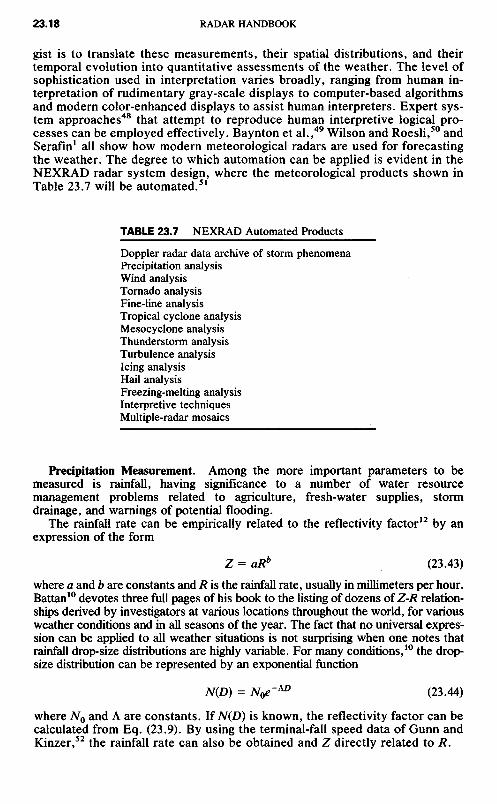
Tornado Detection. A single doppler radar can only measure the radial com-ponent of the vector wind field. Hence, exact measurements of vector winds at apoint are generally not possible. However, rotating winds or vortices can be de-tected and their intensities measured by simply measuring the change in radial
FIG. 23.3 Measurement of rotation or azimuthal shear in a mesocyclone. The azi-muthal shear is given by Av/AJC = 2vr/ra.
velocity with azimuth angle as shown in Fig. 23.3. The radar scans in azimuth anddetects a couplet in radial velocity at constant range. The azimuthal shear isgiven simply by the expression
dvr 2vr— « — (23.49)ax roc
where x is in the direction orthogonal to the radius r and d is the angle subtendedby the circulation at range r.
Because mesocyclones, which spawn tornadoes, can be many kilometers indiameter, radars with 1° beams have the spatial resolution to detectmesocyclones at ranges in excess of 60 km. It should be clear that any meantranslational motion would change the absolute values of the measured radialvelocities but would not affect the shear measurement. Armstrong andDonaldson62 were the first to use shear for severe storm detection. Azimuthalshear values of the order of 10~2 s"1 or greater and with vertical extent greaterthan the diameter of the mesocyclone are deemed necessary for a tornado tooccur.63
Detection of the tornado vortex itself is not generally possible, since its hori-zontal extent may be only a few hundred meters. Detection of the radial shear,therefore, is not possible unless the tornado is close enough to the radar to beresolved by the beamwidth. In cases where the tornado falls entirely within thebeam, the doppler spectral width64 may be used to estimate tornadic intensity. Insome cases, both a mesocyclone and its incipient tornado can be detected.Wilson and Roesli50 show an excellent example of a tornado vortex signature(TVS) embedded within a larger mesocyclone.
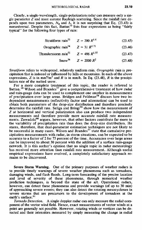
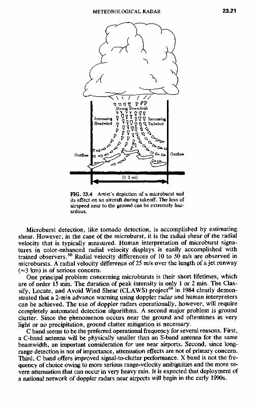
Microbursts. Fujita and Caracena65 first identified the microburst phenome-non as the cause of an airliner crash that took place in 1975. The microburst andits effects on an aircraft during takeoff or landing are depicted in Fig. 23.4. Themicroburst is simply a small-scale, short-duration downdraft emanating from aconvective storm. This ' 'burst" of air spreads out radially as it strikes theground, forming a ring of diverging air about 0.3 to 1 km deep and of the order of2 to 5 km in diameter. Aircraft, penetrating a microburst, experience first an in-crease in head wind and then a continuous, performance-robbing decrease inhead wind, which can cause the plane to crash if encountered shortly beforetouchdown or just as the aircraft is taking off. More complete descriptions ofmicrobursts and their effects on aviation safety are given by Fujita66'67 andMcCarthy and Serafm.68
FIG. 23.4 Artist's depiction of a microburst andits effect on an aircraft during takeoff. The loss ofairspeed near to the ground can be extremely haz-ardous.
Microburst detection, like tornado detection, is accomplished by estimatingshear. However, in the case of the microburst, it is the radial shear of the radialvelocity that is typically measured. Human interpretation of microburst signa-tures in color-enhanced radial velocity displays is easily accomplished withtrained observers.50 Radial velocity differences of 10 to 50 m/s are observed inmicrobursts. A radial velocity difference of 25 m/s over the length of a jet runway(^l km) is of serious concern.
One principal problem concerning microbursts is their short lifetimes, whichare of order 15 min. The duration of peak intensity is only 1 or 2 min. The Clas-sify, Locate, and Avoid Wind Shear (CLAWS) project69 in 1984 clearly demon-strated that a 2-min advance warning using doppler radar and human interpreterscan be achieved. The use of doppler radars operationally, however, will requirecompletely automated detection algorithms. A second major problem is groundclutter. Since the phenomenon occurs near the ground and oftentimes in verylight or no precipitation, ground clutter mitigation is necessary.
C band seems to be the preferred operational frequency for several reasons. First,a C-band antenna will be physically smaller than an S-band antenna for the samebeamwidth, an important consideration for use near airports. Second, since long-range detection is not of importance, attenuation effects are not of primary concern.Third, C band offers improved signal-to-clutter performance. X band is not the fre-quency of choice owing to more serious range-velocity ambiguities and the more se-vere attenuation that can occur in very heavy rain. It is expected that deployment ofa national network of doppler radars near airports will begin in the early 1990s.
IncreasingHeadwind
IncreasingTailwind
OutflowOutflow
Hail. The NEXRAD radar will make use of a hail-detection algorithm similar tothat discussed by Witt and Nelson.70 This algorithm combines high reflectivity factorwith echo height and upper-level radial velocity divergence to detect the occurrenceof hail. Eventually, polarization diversity techniques may improve quantitative haildetection. Aydin, Seliga, and Balaji71 propose a hail-detection technique usingreflectivity measurements at orthogonal polarizations. This technique depends uponthe fact that the ratio of horizontal to vertical reflectivity is unity («0 dB) when hailis present. This differs sharply from heavy rain, where this ratio can be as large as 6dB. The combination of absolute reflectivity factor at horizontal polarization and ra-tio of reflectivities at horizontal and vertical polarizations (differential reflectivity)gives unique signatures for hail and heavy rain, each of which is characterized byhigh reflectivity factor. The difference in the differential reflectivity signatures is eas-ily explained. Large raindrops assume pancakelike shapes as they fall and thus scat-ter back horizontally polarized electric fields more strongly than vertically polarizedelectric fields. Hailstones, while irregular in shape, appear to tumble while they falland therefore exhibit no preferred orientation on average.
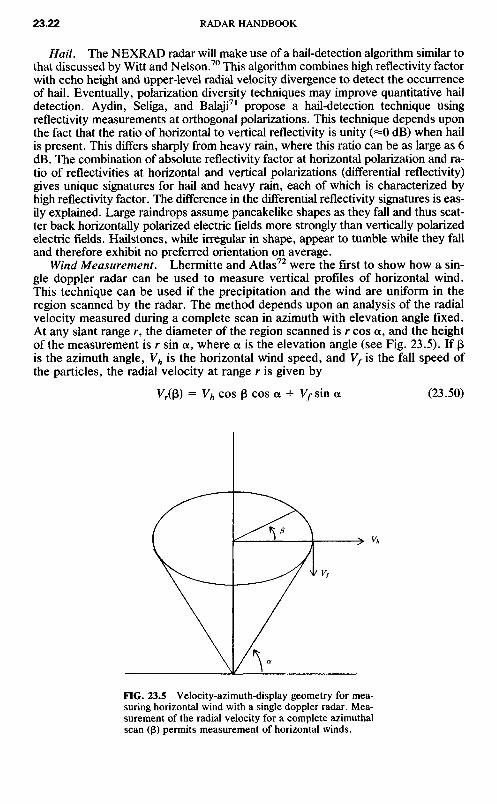
Wind Measurement. Lhermitte and Atlas72 were the first to show how a sin-gle doppler radar can be used to measure vertical profiles of horizontal wind.This technique can be used if the precipitation and the wind are uniform in theregion scanned by the radar. The method depends upon an analysis of the radialvelocity measured during a complete scan in azimuth with elevation angle fixed.At any slant range r, the diameter of the region scanned is r cos a, and the heightof the measurement is r sin a, where a is the elevation angle (see Fig. 23.5). If pis the azimuth angle, Vh is the horizontal wind speed, and Vf is the fall speed ofthe particles, the radial velocity at range r is given by
yr(p) = vh cos p cos a + Vf sin a (23.50)
FIG. 23.5 Velocity-azimuth-display geometry for mea-suring horizontal wind with a single doppler radar. Mea-surement of the radial velocity for a complete azimuthalscan (p) permits measurement of horizontal winds.
A harmonic analysis can be used to obtain Vh, the horizontal wind speed, thewind direction, and V/, the particle fall speed. The technique is referred to as thevelocity-azimuth-display (VAD) technique. Browning and Wexler73 later showedhow the technique could be extended to measure other parameters of the windfield including divergence and deformation. Baynton et al.49 show how the VADcan be applied in real time by using a color-enhanced radial velocity display.
Thunderstorm Prediction. Wilson and Schreiber74 illustrate how modern me-teorological doppler radar can be used to detect locations where new thunder-storm development is likely to occur. Modern radars have sufficient sensitivityto detect clear-air discontinuities in the lower 2 to 4 km of the atmosphere. Prin-cipally, this detection occurs in the summer months. The backscattering mecha-nism may be due to index-of-refraction inhomogeneities caused by turbulence inthe lower layers and/or by insects. Wilson and Schreiber have found that about90 percent of the thunderstorms that occur in the Front Range of the Rockies inthe summertime develop over such boundaries. Since these boundaries can bedetected before any clouds are present and because it is possible to infer the airmass convergence that is taking place along these boundaries through dopplermeasurements, more precise prediction of thunderstorm occurrence appears tobe possible. From the radar designer's standpoint, such applications dictate theuse of antennas with very low sidelobes and signal processors with significantground clutter rejection capability. The NEXRAD radar system, with 50 or moredB of clutter rejection, is well suited to this eventual operational task.
23.6 RESEARCHAPPLICATIONS
Operational meteorological radars are designed for reliability and simplicity ofoperation while providing the performance needed for operational applications.Research radars are considerably more complex, since cutting-edge research re-quires more detailed and more sensitive measurements of a multiplicity of vari-ables simultaneously. In the research community, multiple-parameter radar stud-ies, multiple-doppler radar network studies, and plans for airborne and space-borne radars are all receiving considerable attention.
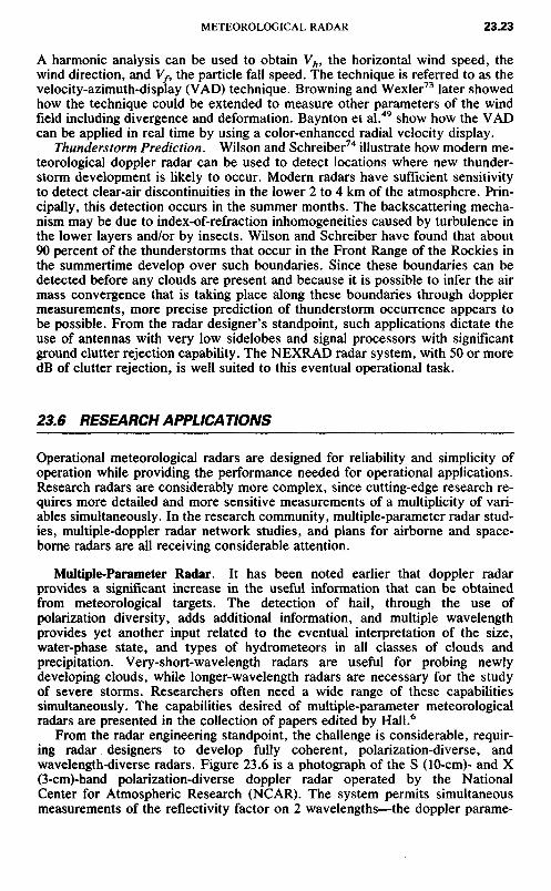
Multiple-Parameter Radar. It has been noted earlier that doppler radarprovides a significant increase in the useful information that can be obtainedfrom meteorological targets. The detection of hail, through the use ofpolarization diversity, adds additional information, and multiple wavelengthprovides yet another input related to the eventual interpretation of the size,water-phase state, and types of hydrometeors in all classes of clouds andprecipitation. Very-short-wavelength radars are useful for probing newlydeveloping clouds, while longer-wavelength radars are necessary for the studyof severe storms. Researchers often need a wide range of these capabilitiessimultaneously. The capabilities desired of multiple-parameter meteorologicalradars are presented in the collection of papers edited by Hall.6
From the radar engineering standpoint, the challenge is considerable, requir-ing radar designers to develop fully coherent, polarization-diverse, andwavelength-diverse radars. Figure 23.6 is a photograph of the S (10-cm)- and X(3-cm)-band polarization-diverse doppler radar operated by the NationalCenter for Atmospheric Research (NCAR). The system permits simultaneousmeasurements of the reflectivity factor on 2 wavelengths—the doppler parame-
FIG. 23.6 The CP-2, multiple-parameter radar at the National Centerfor Atmospheric Research, Boulder, Colorado. (Courtesy of the Na-tional Center for Atmospheric Research.}
ters on a single wavelength, S band, and polarization-diverse measurements atboth wavelengths. The antenna beams are matched with approximately 1°beam widths. The peak transmitted power at S band is 1 MW and 50 kW at Xband. The pulse widths are approximately 1 n,s, and the PRF is typically 1000s"1. The system is characteristic of the technologies currently in place in the re-search community in this field.
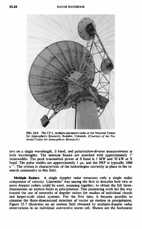
Multiple Radars. A single doppler radar measures only a single radialcomponent of velocity. Lhermitte3 was among the first to describe how two ormore doppler radars could be used, scanning together, to obtain the full three-dimensional air motion fields in precipitation. This pioneering work led the waytoward the use of networks of doppler radars for studies of individual cloudsand larger-scale cloud systems. For the first time, it became possible toexamine the three-dimensional structure of vector air motion in precipitation.Figure 23.7 illustrates an air motion field obtained by multiple-doppler radarobservations in an individual convective storm cell. Shown are the horizontal
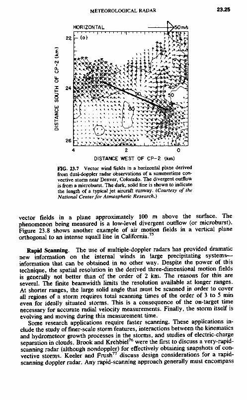
DISTANCE WEST OF CP-2 (km)UG. 23.7 Vector wind fields in a horizontal plane derivedfrom dual-doppler radar observations of a summertime con-vective storm near Denver, Colorado. The divergent outflowis from a microburst. The dark, solid line is shown to indicatethe length of a typical jet aircraft runway. (Courtesy of theNational Center for Atmospheric Research.)
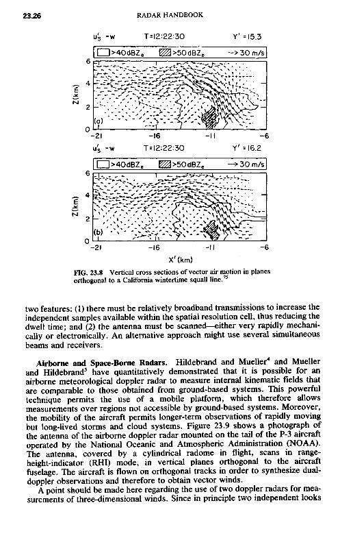
vector fields in a plane approximately 100 m above the surface. Thephenomenon being measured is a low-level divergent outflow (or microburst).Figure 23.8 shows another example of air motion fields in a vertical planeorthogonal to an intense squall line in California.75
Rapid Scanning. The use of multiple-doppler radars has provided dramaticnew information on the internal winds in large precipitating systems-information that can be obtained in no other way. Despite the power of thistechnique, the spatial resolution in the derived three-dimensional motion fieldsis generally not better than of the order of 2 km. The reasons for this areseveral. The finite beamwidth limits the resolution available at longer ranges.At shorter ranges, the large solid angle that must be scanned in order to coverall regions of a storm requires total scanning times of the order of 3 to 5 mineven for ideally situated storms. This is a consequence of the on-target timenecessary for accurate radial velocity measurements. Finally, the storm itself isevolving and moving during this measurement time.
Some research applications require faster scanning. These applications in-clude the study of finer-scale storm features, interactions between the kinematicsand hydrometeor growth processes in the storms, and studies of electric-chargeseparation in clouds. Brook and Krehbiei76 were the first to discuss a very-rapid-scanning radar (although nondoppler) for effectively obtaining snapshots of con-vective storms. Keeler and Frush77 discuss design considerations for a rapid-scanning doppler radar. Any rapid-scanning approach generally must encompass
HORIZONTAL
DIST
ANCE
SOU
TH O
F C
P-2
(km
)
X'(km)FIG. 23.8 Vertical cross sections of vector air motion in planesorthogonal to a California wintertime squall line.75
two features: (1) there must be relatively broadband transmissions to increase theindependent samples available within the spatial resolution cell, thus reducing thedwell time; and (2) the antenna must be scanned—either very rapidly mechani-cally or electronically. An alternative approach might use several simultaneousbeams and receivers.
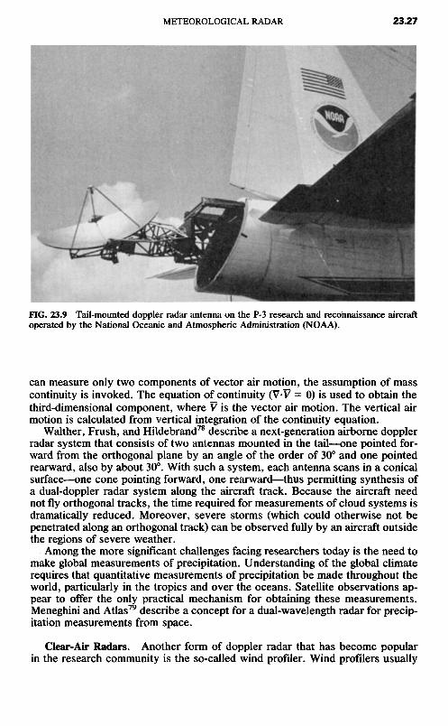
Airborne and Space-Borne Radars. Hildebrand and Mueller4 and Muellerand Hildebrand5 have quantitatively demonstrated that it is possible for anairborne meteorological doppler radar to measure internal kinematic fields thatare comparable to those obtained from ground-based systems. This powerfultechnique permits the use of a mobile platform, which therefore allowsmeasurements over regions not accessible by ground-based systems. Moreover,the mobility of the aircraft permits longer-term observations of rapidly movingbut long-lived storms and cloud systems. Figure 23.9 shows a photograph ofthe antenna of the airborne doppler radar mounted on the tail of the P-3 aircraftoperated by the National Oceanic and Atmospheric Administration (NOAA).The antenna, covered by a cylindrical radome in flight, scans in range-height-indicator (RHI) mode, in vertical planes orthogonal to the aircraftfuselage. The aircraft is flown on orthogonal tracks in order to synthesize dual-doppler observations and therefore to obtain vector winds.
A point should be made here regarding the use of two doppler radars for mea-surements of three-dimensional winds. Since in principle two independent looks
FIG. 23.9 Tail-mounted doppler radar antenna on the P-3 research and reconnaissance aircraftoperated by the National Oceanic and Atmospheric Administration (NOAA).
can measure only two components of vector air motion, the assumption of masscontinuity is invoked. The equation of continuity (V-V = O) is used to obtain thethird-dimensional component, where V is the vector air motion. The vertical airmotion is calculated from vertical integration of the continuity equation.
Walther, Frush, and Hildebrand78 describe a next-generation airborne dopplerradar system that consists of two antennas mounted in the tail—one pointed for-ward from the orthogonal plane by an angle of the order of 30° and one pointedrearward, also by about 30°. With such a system, each antenna scans in a conicalsurface—one cone pointing forward, one rearward—thus permitting synthesis ofa dual-doppler radar system along the aircraft track. Because the aircraft neednot fly orthogonal tracks, the time required for measurements of cloud systems isdramatically reduced. Moreover, severe storms (which could otherwise not bepenetrated along an orthogonal track) can be observed fully by an aircraft outsidethe regions of severe weather.
Among the more significant challenges facing researchers today is the need tomake global measurements of precipitation. Understanding of the global climaterequires that quantitative measurements of precipitation be made throughout theworld, particularly in the tropics and over the oceans. Satellite observations ap-pear to offer the only practical mechanism for obtaining these measurements.Meneghini and Atlas79 describe a concept for a dual-wavelength radar for precip-itation measurements from space.
Clear-Air Radars. Another form of doppler radar that has become popularin the research community is the so-called wind profiler. Wind profilers usually
take the form of VHF and UHF fixed-beam systems, pointing vertically and atangles approximately 15° from the zenith. Such radars7 can make dopplermeasurements throughout the range of altitudes from a few hundred meters to15 km above the surface, depending upon the wavelength selected and thepower-aperture product available. Very powerful radars of this type arereferred to as Mesosphere, Stratosphere, Troposphere (MST) radars because oftheir ability to make measurements throughout most of these atmosphericregions. Powerful MST radars are operated at many laboratories around theworld. Major facilities are located at Kiruna, Sweden; the MassachusettsInstitute of Technology in Cambridge, Massachusetts; Arecibo, Puerto Rico;Jicamarca, Peru; and at the University of Kyoto in Japan.
These clear-air radars receive energy backscattered from index-of-refractioninhomogeneities due to atmospheric turbulence. The antenna systems usuallytake the form of phased arrays. Transmitters are generally in the form of high-powered, fully coherent transmitting tubes. One exception is at the University ofKyoto, where the antenna-transmitter system consists of more than 400 radiatingelements, each with its own solid-state transmitter. This approach allows for fullelectronic scanning of the beam. A network of 400-MHz wind profilers in the cen-tral United States is also expected to use solid-state transmitters, but electronicscanning will not be possible.
The meteorological community is excited about these devices because of theirability to measure winds continuously. This capability permits the observation ofsmaller-scale temporal and spatial wind-field features than can be obtained fromthe global 12-hourly rawindsonde (balloon) networks. These smaller-scale mea-surements are important for understanding local and regional weather and for ef-fective forecasting on these scales.
It is important to recognize that two-beam systems can measure horizontalwinds if the wind field is uniform and if vertical velocities are negligible. A three-beam system can measure all three velocity components if the wind is uniform.Four- and five-beam systems allow one to determine the quality of the measure-ments by detecting the presence of nonuniformity. Carbone, Strauch, andHeymsfield80 and Strauch et al.81 address the issue of wind measurement error indetail.
The reader is referred to the review paper by Rottger and Larsen82 for a thor-ough treatment of wind-profiler technology.
Synthetic Aperture Radar and Pulse Compression. Metcalf and Holm83 andAtlas and Moore84 have considered the use of synthetic aperture radar (SAR)in order to obtain high-resolution measurements from mobile airborne or space-borne platforms. In general, both papers conclude that the cross-beamresolution possible is inherently limited by the decorrelation time of the targetsdue to their turbulent motion. Consequently, SAR offers little advantage overreal aperture systems for meteorological applications from aircraft. However,space-borne systems can effectively use SAR because of the high speed of theorbiting spacecraft.
Pulse compression is not generally used for meteorological applications be-cause peak power is not usually a limitation on system performance. Keeler andFrush,77 however, point out that pulse compression can be of benefit in somerapid-scanning applications. In situations where signals are very weak (such asfor MST applications), pulse compression is used to increase system sensitivityby increasing the average power of the system.
A note of caution is in order when considering pulse compression for meteo-rological radars. This relates to the matter of range sidelobes. Careful design isnecessary to minimize these sidelobes, just as antenna sidelobes should be min-imized, in order to mitigate the effects of interpretive errors caused by wide-dynamic-range distributed weather targets.
REFERENCES
1. Serafin, R. J.: New Nowcasting Opportunities Using Modern Meteorological Radar,Proc. Mesoscale Analysis Forecast. Symp., pp. 35-41, European Space Agency, Paris,1987.
2. McCarthy, J., J. Wilson, and T. T. Fujita: The Joint Airport Weather Studies (JAWS)Project, Bull. Am. Meteorol. Soc., vol. 63, pp. 15-22, 1982.
3. Lhermitte, R. M.: Dual-Doppler Radar Observations of Convective Storm Circula-tions, Preprints, 14th Conf. Radar Meteorol., pp. 139-144, American MeteorologicalSociety, Boston, 1970.
4. Hildebrand, P., and C. Mueller: Evaluation of Meteorological Airborne Doppler Radar,Part I: Dual-Doppler Analyses of Air Motions, J. Atmos. Ocean. TechnoL, vol. 2, pp.362-380, 1985.
5. Mueller, C., and P. Hildebrand: Evaluation of Meteorological Airborne Doppler Radar,Part H: Triple-Doppler Analysis of Air Motions, /. Atmos. Ocean. TechnoL, vol. 2, pp.381-392, 1985.
6. Hall, M. (ed.): Special papers: Multiple Parameter Radar Measurements of Precipita-tion, Radio Sd., vol. 19, 1984.
7. Strauch, R. G., D. A. Merritt, K. P. Moran, K. B. Earnshaw, and D. Van De Kamp: TheColorado Wind Profiling Network, J. Atmos. Ocean. TechnoL, vol. 1, pp. 37-49, 1984.
8. Serafin, R. J., and R. Strauch: Meteorological Radar Signal Processing, in "Air QualityMeteorology and Atmospheric Ozone," American Society for Testing and Materials,Philadelphia, 1977, pp. 159^182.
9. Gray, G. R., R. J. Serafin, D. Atlas, R. E. Rinehart, and J. J. Boyajian: Real-TimeColor Doppler Radar Display, Bull. Am. Meteorol. Soc., vol. 56, pp. 580-588, 1975.
10. Battan, L. J.: "Radar Observation of the Atmosphere," University of Chicago Press,1973.
11. Doviak, R. J., and D. S. Zrni£: "Doppler Radar and Weather Observations," Aca-demic Press, Orlando, FIa., 1984.
12. Bean, B. R., E. J. Dutton, and B. D. Warner: Weather Effects on Radar, in Skolnik, M.(ed.): "Radar Handbook," McGraw-Hill Book Company, New York, 1970, pp.24-1-24-40.
13. Mie, G.: Beitrage zur Optik triiber Medien, speziell kolloidaler Metallosungen [Contri-bution to the optics of suspended media, specifically colloidal metal suspensions], Ann.Phys., vol. 25, pp. 377-445, 1908.
14. Probert-Jones, J. R.: The Radar Equation in Meteorology, Q. J. R. Meteorol. Soc., vol.88, pp. 485-495, 1962.
15. Metcalf, J. L: Airborne Weather Radar and Severe Weather Penetration, Preprints, 19thConf. Radar Meteorol., pp. 125-129, American Meteorological Society, Boston, 1980.
16. Allen, R. H., D. W. Burgess, and R. J. Donaldson, Jr.: Severe 5-cm Radar Attenuationof the Wichita Falls Storm by Intervening Precipitation, Preprints, 19th Conf. RadarMeteorol., pp. 87-89, American Meteorological Society, Boston, 1980.
17. Eccles, P. J., and D. Atlas: A Dual-Wavelength Radar Hail Detector, J. Appl.Meteorol., vol. 12, pp. 847-854, 1973.
18. Donaldson, R. J., Jr.: The Measurement of Cloud Liquid-Water Content by Radar, J.MeteoroL, vol. 12, pp. 238-244, 1955.
19. Weickmann, H. K., and H. J. aufm Kampe: Physical Properties of Cumulus Clouds, J.MeteoroL, vol. 10, pp. 204-221, 1953.
20. Gunn, K. L. S., and T. W. R. East: The Microwave Properties of Precipitation Parti-cles, Q. J. R. MeteoroL Soc., vol. 80, pp. 522-545, 1954.
21. Ryde, J. W., and D. Ryde: "Attenuation of Centimeter Waves by Rain, Hail, Fog, andClouds," General Electric Company, Wembley, England, 1945.
22. Bean, B. R., and R. Abbott: Oxygen and Water Vapor Absorption of Radio Waves inthe Atmosphere, Geofis. Pura AppL, vol. 37, pp. 127-144, 1957.
23. Ryde, J. W.: The Attenuation and Radar Echoes Produced at Centimetre Wavelengthsby Various Meteorological Phenomena, in "Meteorological Factors in Radio WavePropagation," Physical Society, London, 1946, pp. 169-188.
24. Laws, J. O., and D. A. Parsons: The Relationship of Raindrop Size to Intensity, Trans.Am. Geophys. Union, 24th Annual Meeting, pp. 452-460, 1943.
25. Schelleng, J. C., C. R. Burrows, and E. B. Ferrell: Ultra-Short-Wave Propagation,Proc. IRE, vol. 21, pp. 427-463, 1933.
26. Medhurst, R. G.: Rainfall Attenuation of Centimeter Waves: Comparison of Theoryand Measurement, IEEE Trans., vol. AP-13, pp. 550-564, 1965.
27. Burrows, C. R., and S. S. Attwood: "Radio Wave Propagation, Consolidated Sum-mary Technical Report of the Committee on Propagation, NDRC," Academic Press,New York, 1949, p. 219.
28. Humphreys, W. J.: "Physics of the Air," McGraw-Hill Book Company, New York,1940, p. 82.
29. Atlas, D., and E. Kessler III: A Model Atmosphere for Widespread Precipitation,Aeronaut. Eng. Rev., vol. 16, pp. 69-75, 1957.
30. Dennis, A. S.: Rainfall Determinations by Meteorological Satellite Radar, Stanford Re-search Institute, SRIRept. 4080, 1963.
31. Kerker, M., M. P. Langleben, and K. L. S. Gunn: Scattering of Microwaves by a Melt-ing Spherical Ice Particle, /. MeteoroL, vol. 8, p. 424, 1951.
32. "Glossary of Meteorology," vol. 3, American Meteorological Society, Boston, 1959, p.613.
33. Best, A. C.: "Physics in Meteorology," Sir Isaac Pitman & Sons, Ltd., London, 1957.34. Saxton, J. A., and H. G. Hopkins: Some Adverse Influences of Meteorological Factors
on Marine Navigational Radar, Proc. IEE (London), vol. 98, pt. Ill, p. 26, 1951.35. Pasqualucci, F., B. W. Bartram, R. A. Kropfli, and W. R. Moninger: A Millimeter-
Wavelength Dual-Polarization Doppler Radar for Cloud and Precipitation Studies, J.dim. AppL MeteoroL, vol. 22, pp. 758-765, 1983.
36. Lhermitte, R.: A 94-GHz Doppler Radar for Cloud Observations, /. Atmos. Ocean.TechnoL, vol. 4, pp. 36-48, 1987.
37. Richter, J. H.: High-Resolution Tropospheric Radar Sounding, Proc. Colloq. SpectraMeteoroL Variables, Radio ScL, vol. 4, pp. 1261-1268, 1969.
38. Tang Dazhang, S. G. Geotis, R. E. Passarelli, Jr., A. L. Hansen, and C. L. Frush:Evaluation of an Alternating PRF Method for Extending the Range of UnambiguousDoppler Velocity, Preprints, 22d Conf. Radar MeteoroL, pp. 523-527, American Me-teorological Society, Boston, 1984.
39. Laird, B. G.: On Ambiguity Resolution by Random Phase Processing, Preprints, 20thConf. Radar MeteoroL, p. 327, American Meteorological Society, Boston, 1981.
40. Rummler, W. D.: Introduction of a New Estimator for Velocity Spectral Parameters,Tech. Memo. MAf-68-4121-5, Bell Telephone Laboratories, Whippany, N.J., 1968.
41. Hildebrand, P. H., and R. H. Sekhon: Objective Determination of the Noise Level inDoppler Spectra. /. Appl. MeteoroL, vol. 13, pp. 808-311, 1974.
42. Denenberg, J. N., R. J. Serafin, and L. C. Peach: Uncertainties in Coherent Measure-ment of the Mean Frequency and Variance of the Doppler Spectrum from Meteorolog-ical Echoes, Preprints, 15th Conf. Radar MeteoroL, pp. 216-221, American Meteoro-logical Society, Boston, 1972.
43. Davenport, W. B., Jr., and W. L. Root: '4An Introduction to the Theory of RandomSignals and Noise," McGraw-Hill Publishing Company, New York, 1958.
44. Zrnic, D. S.: Estimation of Spectral Moments for Weather Echoes, IEEE Trans., vol.GE-17, pp. 113-128, 1979.
45. Marshall, J. S., and W. Hitschfeld: The Interpretation of the Fluctuating Echo for Ran-domly Distributed Scatterers, pt. I, Can. J. Phys., vol. 31, pp. 962-994, 1953.
46. Frush, C.: Doppler Signal Processing Using IF Limiting, Preprints, 20th Conf. RadarMeteoroL, pp. 332-337, American Meteorological Society, Boston, 1981.
47. Mueller, E. A., and E. J. Silha: Unique Features of the CHILL Radar System,Preprints, 18th Conf. Radar MeteoroL, pp. 381-386, American Meteorological Society,Boston, 1978.
48. Campbell, S. D., and S. H. Olson: Recognizing Low-Altitude Wind Shear Hazardsfrom Doppler Weather Radar: An Artificial Intelligence Approach, J. Atmos. Ocean.TechnoL, vol. 4, p. 518, 1987.
49. Baynton, H. W., R. J. Serafin, C. L. Frush, G. R. Gray, P. V. Hobbs, R. A. Houze,Jr., and J. D. Locatelli: Real-Time Wind Measurement in Extratropical Cyclones byMeans of Doppler Radar, /. Appl. MeteoroL, vol. 16, pp. 1022-1028, 1977.
50. Wilson, J., and H. P. Roesli: Use of Doppler Radar and Radar Networks in MesoscaleAnalysis and Forecasting, ESA J., vol. 9, pp. 125-146, 1985.
51. Bonewitz, J. D.: The NEXRAD Program—An Overview, Preprints, 20th Conf. RadarMeteoroL, pp. 757-761, American Meteorological Society, Boston, 1981.
52. Gunn, R., and Kinzer, G. D.: The Terminal Velocity of Fall for Water Droplets in Stag-nant Air, J. MeteoroL, vol. 6, pp. 243-248, 1949.
53. Marshall, J. S., and W. M. K. Palmer: The Distribution of Raindrops with Size, J.MeteoroL, vol. 4, pp. 186-192, 1948.
54. Blanchard, D. C.: Raindrop Size Distribution in Hawaiian Rains, J. MeteoroL, vol. 10,pp. 457-473, 1953.
55. Jones, D. M. A.: 3 cm and 10 cm Wavelength Radiation Backscatter from Rain, Proc.Fifth Weather Radar Conf., pp. 281-285, American Meteorological Society, Boston,1955.
56. Gunn, K. L. S., and J. S. Marshall: The Distribution with Size of Aggregate Snow-flakes, J. MeteoroL, vol. 15, pp. 452-466, 1958.
57. Wilson, J. W., and E. A. Brandes: Radar Measurement of Rainfall—A Summary, Bull.Am. MeteoroL Soc., vol. 60, pp. 1048-1058, 1979.
58. Bridges, J., and J. Feldman: An Attenuation Reflectivity Technique to Determine theDrop Size Distribution of Water Clouds and Rain, J. Appl. MeteoroL, vol. 5, pp.349-357, 1966.
59. Seliga, T. A., and V. N. Bringi: Potential Use of Radar Differential Reflectivity Mea-surements at Orthogonal Polarizations for Measuring Precipitation, J. Appl. MeteoroL,vol. 15, pp. 69-76, 1976.
60. Zawadzki, L: Factors Affecting the Precision of Radar Measurements of Rain,Preprints, 22d Conf. Radar MeteoroL, pp. 251-256, American Meteorological Society,Boston, 1984.
61. Burgess, D., et al.: Final Report on the Joint Doppler Operational Project (JDOP),1976-1978, NOAA Tech. Memo. ERL NSSL-S6, 1979.
62. Armstrong, G. M., and R. J. Donaldson, Jr.: Plan Shear Indicator for Real-TimeDoppler Identification of Hazardous Storm Winds, J. Appl. MeteoroL, vol. 8, pp.376-383, 1969.
63. Donaldson, R. J., Jr.: Vortex Signature Recognition by a Doppler Radar, J. Appl.MeteoroL, vol. 9, pp. 661-670, 1970.
64. Zrni£, D. S., and R. J. Doviak: Velocity Spectra of Vortices Scanned with a PulseDoppler Radar, J. Appl. MeteoroL, vol. 14, pp. 1531-1539, 1975.
65. Fujita, T., and F. Caracena: An Analysis of Three Weather-Related Aircraft Accidents,Bull. Am. MeteoroL Soc., vol. 58, pp. 1164-1181, 1977.
66. Fujita, T.: 'The Downburst," Satellite and Mesometeorology Research Project, De-partment of the Geophysical Sciences, University of Chicago, 1985.
67. Fujita, T.: "The DFW Microburst," Satellite and Meteorology Research Project, De-partment of the Geophysical Sciences, University of Chicago, 1986.
68. McCarthy, J., and R. Serafin: The Microburst: Hazard to Aviation, Weatherwise, vol.37, no. 3, pp. 120-127, 1984.
69. McCarthy, J., J. Wilson, and M. Hjelmfelt: Operational Wind Shear Detection andWarning: The CLAWS Experience at Denver and Future Objectives, Preprints, 23dConf. Radar MeteoroL, pp. 22-26, American Meteorological Society, Boston, 1986.
70. Witt, A., and S. P. Nelson: The Relationship between Upper-Level Divergent OutflowMagnitude as Measured by Doppler Radar and Hailstorm Intensity, Preprints, 22dConf. Radar MeteoroL, pp. 108-111, American Meteorological Society, Boston, 1984.
71. Aydin, K., T. A. Seliga, and V. Balaji: Remote Sensing of Hail with a Dual LinearPolarization Radar, J. dim. Appl. MeteoroL, vol. 25, pp. 1475-1484, 1986.
72. Lhermitte, R. M., and D. Atlas: Precipitation Motion by Pulse Doppler Radar, Proc.Ninth Weather Radar Conf., pp. 218-223, American Meteorological Society, Boston,1961.
73. Browning, K. A., and R. Wexler: A Determination of Kinematic Properties of a WindField Using Doppler Radar, J. Appl. MeteoroL, vol. 7, pp. 105-113, 1968.
74. Wilson, J. W., and W. E. Schreiber: Initiation of Convective Storms at Radar-Observed Boundary Layer Convergence Lines, Mon. Weather Rev., vol. 114, pp.2516-2536, 1986.
75. Carbone, R. E.: A Severe Frontal Rainband, Part I: Storm-Wide Hydrodynamic Struc-ture, /. Atmos. Sd., vol. 39, pp. 258-279, 1982.
76. Brook, M., and P. Krehbiel: A Fast-Scanning Meteorological Radar, Preprints, 16thConf. Radar MeteoroL, pp. 26-31, American Meteorological Society, Boston, 1975.
77. Keeler, R. J., and C. L. Frush: Rapid-Scan Doppler Radar Development Consider-ations, Part II: Technology Assessment, Preprints, 21st Conf. Radar MeteoroL, pp.284-290, American Meteorological Society, Boston, 1983.
78. Walther, C., C. Frush, and P. Hildebrand: The NCAR Airborne Doppler Radar, PartIII: Overview of Radar Design Details, Preprints, 23d Conf. Radar MeteoroL, vol. I,pp. 155-158, American Meteorological Society, Boston, 1986.
79. Meneghini, R., and D. Atlas: Simultaneous Ocean Cross-Section and Rainfall Measure-ments from Space with a Nadir-Looking Radar, J. Atmos. Ocean. TechnoL, vol. 3, pp.400-413, 1986.
80. Carbone, R. E., R. Strauch, and G. M. Heymsfield: Simulation of Wind Profilers inDisturbed Conditions, Preprints, 23d Conf. Radar MeteoroL, vol. I, pp. 44—47,American Meteorological Society, Boston, 1986.
81. Strauch, R. G., B. L. Weber, A. S. Frisch, C. G. Little, D. A. Merritt, K. P. Moran,and D. C. Welsh: The Precision and Relative Accuracy of Profiler Wind Measure-ments, J. Atmos. Ocean. TechnoL, vol. 4, pp. 563-571, 1987.
82. Rottger, J., and M. F. Larsen: Clear Air Radar Techniques, invited paper, 40th Conf.
Radar MeteoroL, American Meteorological Society, Boston, 1987. Published in Atlas,D. (ed.): "Radar Meteorology," American Meteorological Society, Boston, 1989.
83. Metcalf, J. L, and W. A. Holm: Meteorological Applications of Synthetic Aperture Ra-dar, final report, Project A-2101, Engineering Experiment Station, Georgia Institute ofTechnology, 1979.
84. Atlas, D., and R. K. Moore: The Measurement of Precipitation with Synthetic Aper-ture Radar, J. Atmos. Ocean. Technol., vol. 4, pp. 368-376, 1987.