42

CHAPTER 3

ANALYSIS OF LOAD FLOW PROBLEM USING

GENETIC ALGORITHM

3.1 INTRODUCTION

The trend, which appears in the development of modern

transmission systems, is the more intensive utilization of existing networks.

In addition to this, due to deregulation and reconstruction of the electric

power industry, the need arises to transport large blocks of power between

areas through defined corridors. Further more, the voltage profile of the

remote buses of systems is necessary to be kept within a pre-specified range.

Load flow is a solution for the static operating condition of an electric power

system. Since the load flow equation is algebraic non-linear, many numerical

methods have been developed for finding the desired normal solutions.

It is used to determine (i) Equipment rating; (ii) Electrical

Equipment Loading and system loses (iii) Bus voltage magnitude and angles

and (iv) Reactive power support requirements to maintain voltages within

limits for a given scenario and a contingency. All the above methods need an

initial guess value to start. The random selection of initial value may cause the

methods to miss the normal solution.

Recently, there has been much interest in the application of

stochastic search methods, such as genetic algorithm, to solve the power

system problems. Genetic Algorithm is a computerized search and

43

optimization algorithm based on the mechanics of natural genetics and natural

selection. GA is very different from traditional search and optimization

methods used in engineering problems. Because of the simplicity, ease of

operation, minimum requirements and global perspective, GA’s have been

successfully used in a wide variety of problems. Genetic Algorithm is a part

of evolutionary computing, which is rapidly growing area of artificial

intelligence. GA and its modified versions have been popular because of

solving highly nonlinear optimization problems.

3.2 GENETIC ALGORITHM

Genetic Algorithm was first proposed by Holland in the early 1970s

and put into practical applications in the late 1980s. In power systems, GA

has been applied for optimization of generation expansion planning, economic

dispatch unit commitment and a reactive power planning. GAs are random

search optimization algorithm based on the mechanics of natural selection and

genetics (Sheble et al 1995). The objective of GA is to find the optimal

solution to a problem. Since GAs have heuristic procedures, they are not

guaranteed to find the optimum, but experience has shown that they are able

to find very good solutions for a wide range of problems. They operate on

string structures, typically a concatenated list of binary digits representing a

coding of the parameters for a given problem. GAs differ from more

traditional optimization techniques in four important ways (Sudhakaran et al

2004, Lai et al 1997). They are

a) GAs use objective function information to guide the search,

not derivative or other auxiliary information.

b) GAs use a coding of the parameters used to calculate the

objective function in guiding the search, not the parameter

themselves.

44

c) GAs search through many points in the solution space at one

time, not a single point.

d) GAs use probabilistic rules, not deterministic rules, in moving

from one set of solutions to the next.

Reproduction or selection, crossover and mutation are the three

important GA operators (Lai et al 1997). Parent selection is a process where

two chromosomes are selected from the parent population based on their

fitness value. Solutions with high fitness values have a high probability of

contributing new offspring to the next generation (Maifeld et al 1996). The

function of crossover is the creation of new individuals, out of two individuals

of the current population (Sudhakaran et al 2004). Mutation is the operator

responsible for the injection of new information. With a small probability,

random bits of the offspring chromosomes flip from 0 to 1 and vice versa and

give the new characteristic that do not exist in the parent population (Bakirtzis

et al 2002). The flow chart for the simple GA is given in the Appendix 1 in

Figure A1.2.

It is widely recognized that the Simple Genetic Algorithm (SGA)

scheme is capable of locating the neighborhood of the optimal or near optimal

solutions, but in general, requires a large number of generations to converge.

This problem becomes more intense for large-scale optimization problems

with difficult search spaces and lengthy chromosomes, where the possibility

for the SGA to get trapped in local optima increases and convergence speed

of the SGA decreases. At this point, a suitable combination of the basic and

advanced genetic operators must be introduced in order to enhance the

performance of the SGA.

45

3.3 ANALYSIS OF LOAD FLOW PROBLEM USING FAST

SEARCH GENETIC ALGORITHM

3.3.1 Introduction

In this research work, Fast Search Genetic Algorithm is used to find

the solution of load flow problem. FSGA overcomes the drawbacks of

conventional methods. It involves the simple genetic operators and the

advanced features like fitness scaling, elitism and hill climbing. This will

explore the problem search space and gives the better solution. Hill climbing

operator will increase the speed of convergence. Test results on Ward Hale

Six Bus system demonstrate the improvement achieved with the aid of

advanced operators.

3.3.2 Fast Search Genetic Algorithm (FSGA)

In this thesis, Fast Search Genetic Algorithm is used to solve the

load flow problem because of its simplicity and global or near global solution

to the problem. The objective function is to minimize the summation of

square of the change in real and reactive power and change in voltage (for PV

bus only).

One of the most important issues in the genetic evolution is the

effective rearrangement of the genotype information. In the SGA, crossover is

the main genetic operator responsible for the exploitation of information

while mutation brings new nonexistent bit structures. It is widely recognized

that the SGA scheme is capable of locating the neighborhood of the optimal

or near optimal solutions, but in general, requires a large number of

generations to converge. This problem becomes more intense for large-scale

optimization problems with difficult search spaces and lengthy chromosomes.

At this point, a suitable combination of the basic and advanced genetic

46

operators must be introduced in order to enhance the performance of the

SGA. Advanced genetic operators usually combine local search techniques

and expertise derived from the nature of the problem.

A set of advanced genetic operators have been added to the SGA in

order to increase its convergence speed and improve the quality of solution.

Our interest was focused on constructing simple yet powerful enhanced

genetic operators that effectively explore the problem search space. The

advanced features included in our GA implementation are

3.3.2.1 Fitness Scaling

In order to avoid early domination of extraordinary strings and to

encourage a healthy competition among equals, a scaling of the fitness of the

population is necessary. In our approach, the fitness is scaled by a linear

transformation.

3.3.2.2 Elitism

Elitism ensures that the best solution found thus far is never lost

when moving from one generation to another. The best solution of each

generation replaces a randomly selected chromosome in new generation.

3.3.2.3 Hill Climbing

In order to increase the GA search speed at smooth areas of the

search space, a hill climbing operator is introduced, which perturbs a

randomly selected control variable. The modified chromosome is accepted if

there is an increase in Fitness Function (FF) value; otherwise, the old

47

chromosome remains unchanged. This operator is applied only to the best

chromosome (elite) of every generation (Bakirtzis et al 2002).

The main difference between SGA and the proposed FSGA is the

addition of advanced operators. The convergence criteria value is different for

SGA and FSGA. The algorithm for the proposed method is

Step1 : Initialize population and Evaluate population.

Step2 : Check the termination criteria. If the criterion is satisfied,

stop the process and print results otherwise go to next step.

Step3 : Apply roulette wheel selection, then apply single point

crossover and then apply mutation operator

Step4 : Apply elitism and hill climbing operator.

Step5 : Evaluate the population.

Step6 : Increment the generation and go to step2.

3.3.3 Problem Formulation

In this work, the problem formulation is in rectangular coordinates

and the variables are in per unit. Consider an interconnected n-node power

system where there are PQn load nodes, PVn voltage controlled nodes and one

slack node. In rectangular coordinates, there are 2(n-1) unknowns to solve.

The load flow equations are

n n

spi i ij j ij j i ij j ij j PQ PV

j 1 j 1

P E G E B F F G F B E i n n

(3.1)

n n

spi i ij j ij j i ij j ij j PQ

j 1 j 1

Q F G E B F F G F B E i n

(3.2)

48

and

2sp 2 2i i i PVV E F i n (3.3)

where i i iV E jF and ij ij ijY G jB

The objective function results from the summation of squares of the

power mismatch and the voltage mismatch whose minimum coincides with

the load flow solution (Youdong et al 1991).

PQ PV PQ PV

2 2 2i i i

i n n i n i nmin g E,F P Q V

(3.4)

Where

Power Mismatch Criteria:

n n

spi i i ij j ij j i ij j ij j PQ PV

j 1 j 1

P P E G E B F F G F B E i n n

(3.5)

n n

spi i i ij j ij j i ij j ij j PQ

j 1 j 1

Q Q F G E B F E G F B E i n

(3.6)

Voltage Mismatch Criteria:

1

sp 2 2 2i i i i PVV V E F i n (3.7)

The load flow objective function is to be minimized, g(E,F), is

transformed and normalized to a fitness scheme to be maximized and is given

by,

1f E,F

g E,F (3.8)

49

3.3.4 Genetic Algorithm Implementation

The application of GA for the solution of Load flow problem is

explained below. The proposed FSGA is tested on the Ward Hale Six bus

system (Pai 1984) including the half line charging admittance and off-nominal

turns ratio.

Step 1: Representation

Representation plays a key note in the development of GA problem

that can be solved once it can be represented in the form of a solution string

(Chromosomes). The bits (genes) in the chromosomes could be binary

numbers. In this thesis work, real part of the voltage (E) and imaginary part of

the voltage (F) are considered to be a variable for the solution of Load flow

problem except the slack bus. The variable E is represented by 5 bits and 4

bits are used to represent the variable F. There are ten variables to solve in

this problem. The length of the string is 45.

Step 2: Initialization

To begin, the initial population is in binary string which is

generated randomly. Then find the decimal value of the binary string from the

following Equation (3.9).

0 1 i chro len0 1 i chro lenvalue bit 2 bit 2 ........ bit 2 ........ bit 2

(3.9)

The decoding value of the variable is computed by the

Equation (3.10)

i i0

1 i chro len

value x max x minx x min

2 1

(3.10)

50

where

x1 is the decoder at real part of the voltage or imaginary part of the

voltage.

xi (min) is the Lower limit of the variable

xi (max) is the Upper limit of the variable

chro-len is the Total length of the string

value is the decimal value equivalent to the binary string.

In this thesis work, on the PQ nodes, the variables were specified in the

intervals (0.9, 1.0) for E and (-0.2, 0.2) for F. On the PV nodes, the variables

were specified in the intervals (0.9, 1.1) for E and (-0.3, 0.3) for F. The

population size is taken as 10.

Step 3: Calculation of fitness value

The fitness function for each variable is determined by finding the

value of objective function to that variable, which is given below:

Fitness function 1f E,F

g E,F

The fitness function is computed for every individual of the

population. In the maximization problem, the string which has higher fitness

value will be the best string.

Step 4: Selection or reproduction

Reproduction selects good strings in a population and forms a

mating pool. Reproduction operator is also called as selection operator. In this

work, Roulette wheel selection is used.

51

Step 5: Cross Over

Cross Over is a mechanism for diversification. The strings to be

crossed and the crossing points are selected randomly and crossover is done

with 0.8 cross over probability. A single point cross over is used in this work.

Step 6: Mutation

Mutation is a random modification of randomly selected string.

Mutation is done with a mutation probability of 0.01.

Step 7: Apply elitism and hill climbing operator, and then evaluate the

population

After completing an iteration of GA, the best value is stored. Then

the strings available at the end of first iteration will be treated as parent

chromosome for the second iteration. The work procedure is repeated until a

convergence criterion is satisfied.

3.3.5 Results and Discussion

The proposed FSGA is tested on the Ward Hale Six bus system

including the half line charging admittance and off-nominal turns ratio. The

data for 6 bus system are given in Appendix 1 in Table A1.1 and A1.2, and

the single line diagram of 6 bus system is given in Appendix 1 in Figure A1.4.

There are 10 variables to solve for the 6 bus system. The variables are Ei and

Fi except the slack bus. On the PQ nodes, the variables were specified in the

intervals [0.9, 1.0] for E and [-0.2, 0.2] for F. The variation of E and F on PV

nodes were constrained in the intervals [0.9, 1.1] and [-0.3, 0.3]. The problem

is solved first by simple genetic algorithm and then by proposed Fast Search

52

Genetic Algorithm. The parameters selected for the solution of above problem

is given in Table 3.1. Both algorithms are implemented using MATLAB

software on a Pentium-4 PC. The best results of four runs for SGA and for

Table 3.1 Parameter Values for SGA and FSGA

Parameters SGA FSGA

Length of the chromosome 45 45

Population size 10 10

Crossover probability 0.8 0.8

Mutation probability 0.01 0.01

Convergence criteria 0.7 0.5

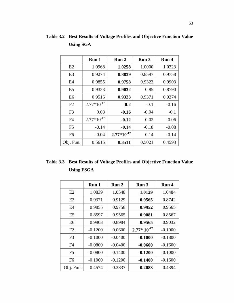
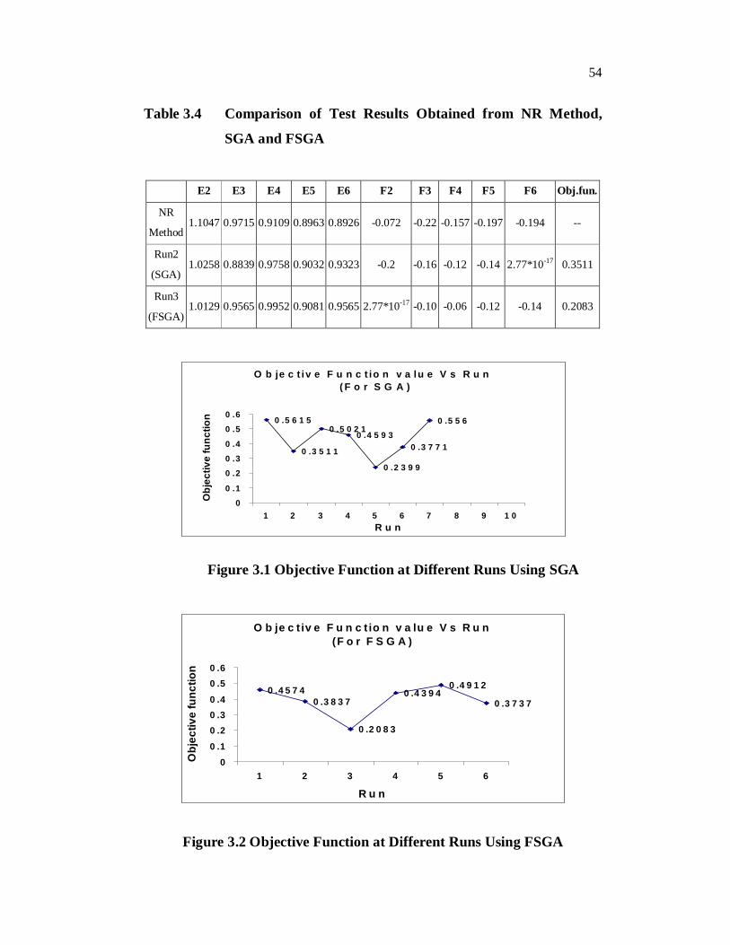
FSGA are tabulated in Tables 3.2 and 3.3 respectively. Results of Run2 from

Table 3.2 and results of Run3 from Table 3.3 are compared with NR method

and are given in Table 3.4. From the comparison of results it is proved that

the FSGA produce improvements in the real voltage profiles than the SGA

and NR method. Especially the FSGA can give near global optimum solution.

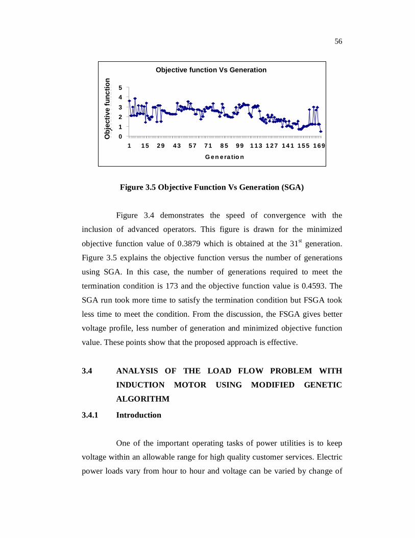
It is also verified that the number of generation required to satisfy

convergence criteria is only 33 for FSGA method and the computer

processing time is around 0.2 seconds. The number of generations to satisfy

the convergence criteria for SGA is 420 and the computer processing time is

around 4 seconds. The objective function value at different runs for SGA and

FSGA are shown in Figure 3.1 and Figure 3.2 respectively. Real voltage

profiles for SGA and FSGA is shown in Figure 3.3.

53

Table 3.2 Best Results of Voltage Profiles and Objective Function Value

Using SGA

Run 1 Run 2 Run 3 Run 4 E2 1.0968 1.0258 1.0000 1.0323 E3 0.9274 0.8839 0.8597 0.9758 E4 0.9855 0.9758 0.9323 0.9903 E5 0.9323 0.9032 0.85 0.8790 E6 0.9516 0.9323 0.9371 0.9274 F2 2.77*10-17 -0.2 -0.1 -0.16 F3 0.08 -0.16 -0.04 -0.1 F4 2.77*10-17 -0.12 -0.02 -0.06 F5 -0.14 -0.14 -0.18 -0.08 F6 -0.04 2.77*10-17 -0.14 -0.14

Obj. Fun. 0.5615 0.3511 0.5021 0.4593

Table 3.3 Best Results of Voltage Profiles and Objective Function Value

Using FSGA

Run 1 Run 2 Run 3 Run 4 E2 1.0839 1.0548 1.0129 1.0484 E3 0.9371 0.9129 0.9565 0.8742 E4 0.9855 0.9758 0.9952 0.9565 E5 0.8597 0.9565 0.9081 0.8567 E6 0.9903 0.8984 0.9565 0.9032 F2 -0.1200 0.0600 2.77* 10-17 -0.1000 F3 -0.1000 -0.0400 -0.1000 -0.1800 F4 -0.0800 -0.0400 -0.0600 -0.1600 F5 -0.0800 -0.1400 -0.1200 -0.1000 F6 -0.1000 -0.1200 -0.1400 -0.1600

Obj. Fun. 0.4574 0.3837 0.2083 0.4394

54

Table 3.4 Comparison of Test Results Obtained from NR Method,

SGA and FSGA

E2 E3 E4 E5 E6 F2 F3 F4 F5 F6 Obj.fun.

NR

Method 1.1047 0.9715 0.9109 0.8963 0.8926 -0.072 -0.22 -0.157 -0.197 -0.194 --

Run2

(SGA) 1.0258 0.8839 0.9758 0.9032 0.9323 -0.2 -0.16 -0.12 -0.14 2.77*10-17 0.3511

Run3

(FSGA) 1.0129 0.9565 0.9952 0.9081 0.9565 2.77*10-17 -0.10 -0.06 -0.12 -0.14 0.2083

O b je c t iv e F u n c t io n v a lu e V s R u n ( F o r S G A )

0 .5 6 1 5

0 .3 5 1 1

0 .5 0 2 10 .4 5 9 3

0 .2 3 9 9

0 .3 7 7 1

0 .5 5 6

0

0 .1

0 .2

0 .3

0 .4

0 .5

0 .6

1 2 3 4 5 6 7 8 9 1 0R u n

Obj

ectiv

e fu

nctio

n

Figure 3.1 Objective Function at Different Runs Using SGA

O b je c t iv e F u n c t io n v a lu e V s R u n (F o r F S G A )

0 .4 5 7 40 .3 8 3 7

0 .2 0 8 3

0 .4 3 9 40 .4 9 1 2

0 .3 7 3 7

00 .1

0 .20 .30 .4

0 .50 .6

1 2 3 4 5 6

R u n

Obj

ectiv

e fu

nctio

n

Figure 3.2 Objective Function at Different Runs Using FSGA

55

R e a l V o lta g e P r o file s fo r v a r io u s b u s e s

00 .20 .40 .60 .8

11 .2

1 2 3 4 5

B u s N u m b e r

Rea

l Vol

tage

F S G A

S G A

Figure 3.3 Real Voltages at Various Buses

From the above table, it is observed that if the SGA method is

applied, the objective function value obtained is greater than the FSGA

method. This is due to premature convergence nature of the SGA method.

Therefore the concepts of elitism and hill climbing are introduced to obtain

the FSGA method. Due to the above advanced operators, the FSGA method

will work efficiently than the SGA method. The FSGA method results better

voltage profiles than the NR method.

Figure 3.4 Objective Function Vs Generation (FSGA)

Objective function Vs Generation

0

0.5

1

1.5

2

1 3 5 7 9 11 13 15 17 19 21 23 25 27 29 31

Generation

Obj

ectiv

e fu

nctio

n

56

O b je c tiv e F u n c tio n v s G e n e ra tio n

012345

1 15 29 43 57 71 8 5 99 1 13 1 27 14 1 155 169

G en era tio n

Obj

ectiv

e Fu

nctio

n

Figure 3.5 Objective Function Vs Generation (SGA)

Figure 3.4 demonstrates the speed of convergence with the

inclusion of advanced operators. This figure is drawn for the minimized

objective function value of 0.3879 which is obtained at the 31st generation.

Figure 3.5 explains the objective function versus the number of generations

using SGA. In this case, the number of generations required to meet the

termination condition is 173 and the objective function value is 0.4593. The

SGA run took more time to satisfy the termination condition but FSGA took

less time to meet the condition. From the discussion, the FSGA gives better

voltage profile, less number of generation and minimized objective function

value. These points show that the proposed approach is effective.

3.4 ANALYSIS OF THE LOAD FLOW PROBLEM WITH

INDUCTION MOTOR USING MODIFIED GENETIC

ALGORITHM

3.4.1 Introduction

One of the important operating tasks of power utilities is to keep

voltage within an allowable range for high quality customer services. Electric

power loads vary from hour to hour and voltage can be varied by change of

Objective function Vs Generation

Obj

ectiv

e fu

nctio

n

57

power load. The classical constant power load model is usually employed for

load flow analysis. Most of the industries use the induction motor loads,

since the actual loads of power systems mostly have non linear voltage

characteristics. There is a need to include the non linear load model into load

flow problem and is essential to get better and precise results of load flow

analysis. The problem related to transient and voltage stabilities due to

dynamic behavior of induction motor loads, have a major area of attraction

for power system planners and operation engineers all over the world. In this

research work, conventional load flow algorithm has been upgraded and

modified to incorporate the nonlinear characteristics of induction motor load.

The modified load flow accounts for the motor slip and scheduled reactive

power that are adjusted during the iteration process. Modified genetic

algorithm (MGA) involves a set of improved operators like Elitism,

tournament selection and two point crossovers, in order to increase its

convergence speed and improve the quality of solution. In MGA, the

objective function is to minimize the voltage and power mismatches and also

constraining the power loss to a minimum value. The implementation of

Modified Genetic Algorithm and its application to a Ward-Hale Six bus

system and a 9 bus system are presented and examined by incorporating an

additional term (real power loss) in the objective function and the normal

solution is found.

3.4.2 Modified Genetic Algorithm (MGA)

In this thesis, Modified Genetic Algorithm is used to solve the load

flow problem with Induction motor load. The objective function is to

minimize the square of the change in real and reactive power, change in

voltage (for PV bus only) and real power loss. A set of improved genetic

operators has been added to the SGA in order to increase its convergence

speed and improve the quality of solution. The advanced features included in

our GA implementation are

58

3.4.2.1 Fitness Scaling

In order to avoid early domination of extraordinary strings and to

encourage a healthy competition among equals, a scaling of the fitness of the

population is necessary. In our approach, the fitness is scaled by a linear

transformation.

3.4.2.2 Elitism

Elitism ensures that the best solution found thus far is never lost

when moving from one generation to another. The best solution of each

generation replaces a randomly selected chromosome in new generation

(Bakirtzis et al 2002).

3.4.2.3 Two Point Crossover

In a two-points cross over operator, two random sites are chosen

and the contents bracketed by these sites are exchanged between two mated

parents. If the cross-site 1 is three and cross-site 2 is six, the strings between

three and six are exchanged as shown in Figure 3.6 (Rajasekaran et al 2003).

cross-site 1 cross-site 2 Parent-1 1 0 0 1 0 1 1 1

Parent-2 0 1 1 1 0 0 0 1

Strings before mating

Child-1 1 0 0 1 0 0 1 1

Child-2 0 1 1 1 0 1 0 1

Strings after mating

Figure 3.6 Two Point Crossover

59

3.4.2.4 Tournament Selection

The fitness proportional selection (e.g. Roulette-wheel selection) is

likely to lead to two problems, namely (Rajasekaran et al 2003).

1. Stagnation of search because it lacks selection pressure, and

2. Premature convergence of the search because it causes the

search to narrow down too quickly.

Unlike the Roulette-wheel selection, the tournament selection

strategy provides selective pressure by holding a tournament competition

among NU Individuals (Frequency of NU =2).The best individual (the winner)

from the tournament is the one with highest fitness Ф which is the winner of

NU. Tournament competitors and the winner are then inserted into the mating

pool. The tournament competition is repeated until the mating pool for

generating new offspring is filled. The mating pool comprising of tournament

winner has higher average population fitness. The fitness difference provides

the selection pressure, which drives GA to improve the fitness of succeeding

genes. The main difference between SGA and the proposed MGA is the

addition of improved operators.

The algorithm for the proposed method is

Step 1 : Initialize population.

Step2 : Check the termination criteria (generation no). If the

generation is greater than the maximum generation, stop

the process and print the results otherwise go to next step.

Step 3 : Evaluate fitness function

Step4 : Apply tournament selection, then apply two point

crossovers and then apply mutation operator.

60

Step 5 : Apply elitism operator.

Step 6 : Increment the generation and go to step2

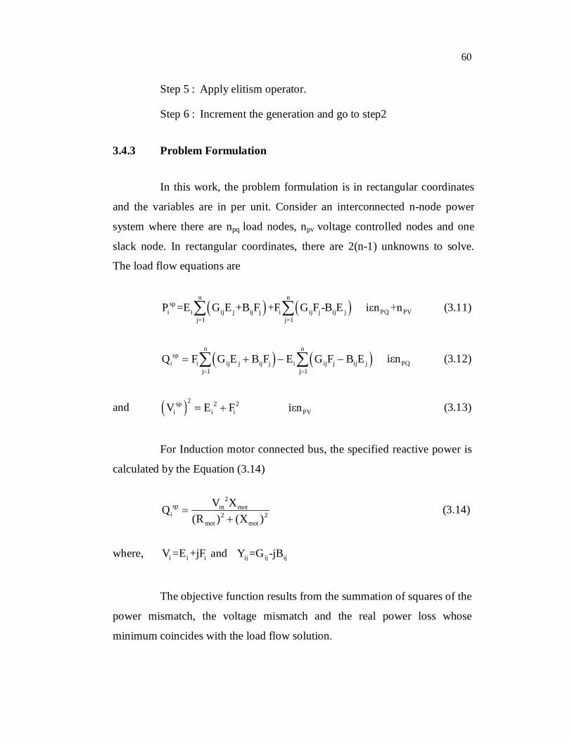
3.4.3 Problem Formulation

In this work, the problem formulation is in rectangular coordinates

and the variables are in per unit. Consider an interconnected n-node power

system where there are npq load nodes, npv voltage controlled nodes and one

slack node. In rectangular coordinates, there are 2(n-1) unknowns to solve.

The load flow equations are

n n

spi i ij j ij j i ij j ij j

j=1 j=1

P =E G E +B F +F G F -B E PQ PViεn +n (3.11)

n n

spi i ij j ij j i ij j ij j

j 1 j 1Q F G E B F E G F B E

PQiεn (3.12)

and 2sp 2 2i i iV E F PViεn (3.13)

For Induction motor connected bus, the specified reactive power is

calculated by the Equation (3.14)

2

sp m moti 2 2

mot mot

V XQ(R ) (X )

(3.14)

where, i i iV =E +jF and ij ij ijY =G -jB

The objective function results from the summation of squares of the

power mismatch, the voltage mismatch and the real power loss whose

minimum coincides with the load flow solution.

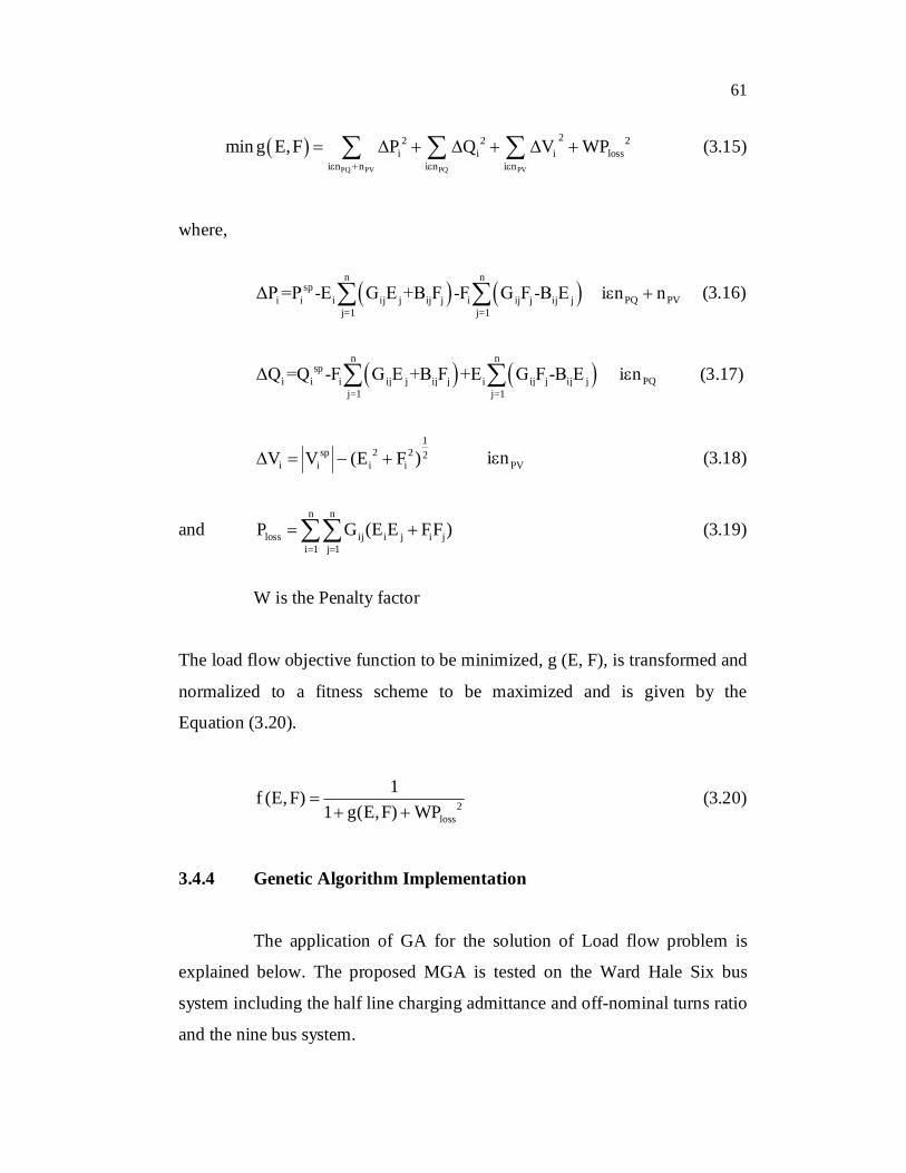
61

PQ PV PQ PV

22 2 2i i i loss

i n n i n i n

min g E,F P Q V WP

(3.15)

where,

n n

spi i i ij j ij j i ij j ij j

j=1 j=1

ΔP =P -E G E +B F -F G F -B E PQ PVi n n (3.16)

n n

spi i i ij j ij j i ij j ij j

j=1 j=1

ΔQ =Q -F G E +B F +E G F -B E PQi n (3.17)

1

sp 2 2 2i i i iV V (E F ) PVi n (3.18)

and n n

loss ij i j i ji 1 j 1

P G (E E FF )

(3.19)

W is the Penalty factor

The load flow objective function to be minimized, g (E, F), is transformed and

normalized to a fitness scheme to be maximized and is given by the

Equation (3.20).

2loss

1f (E,F)1 g(E,F) WP

(3.20)

3.4.4 Genetic Algorithm Implementation

The application of GA for the solution of Load flow problem is

explained below. The proposed MGA is tested on the Ward Hale Six bus

system including the half line charging admittance and off-nominal turns ratio

and the nine bus system.

62

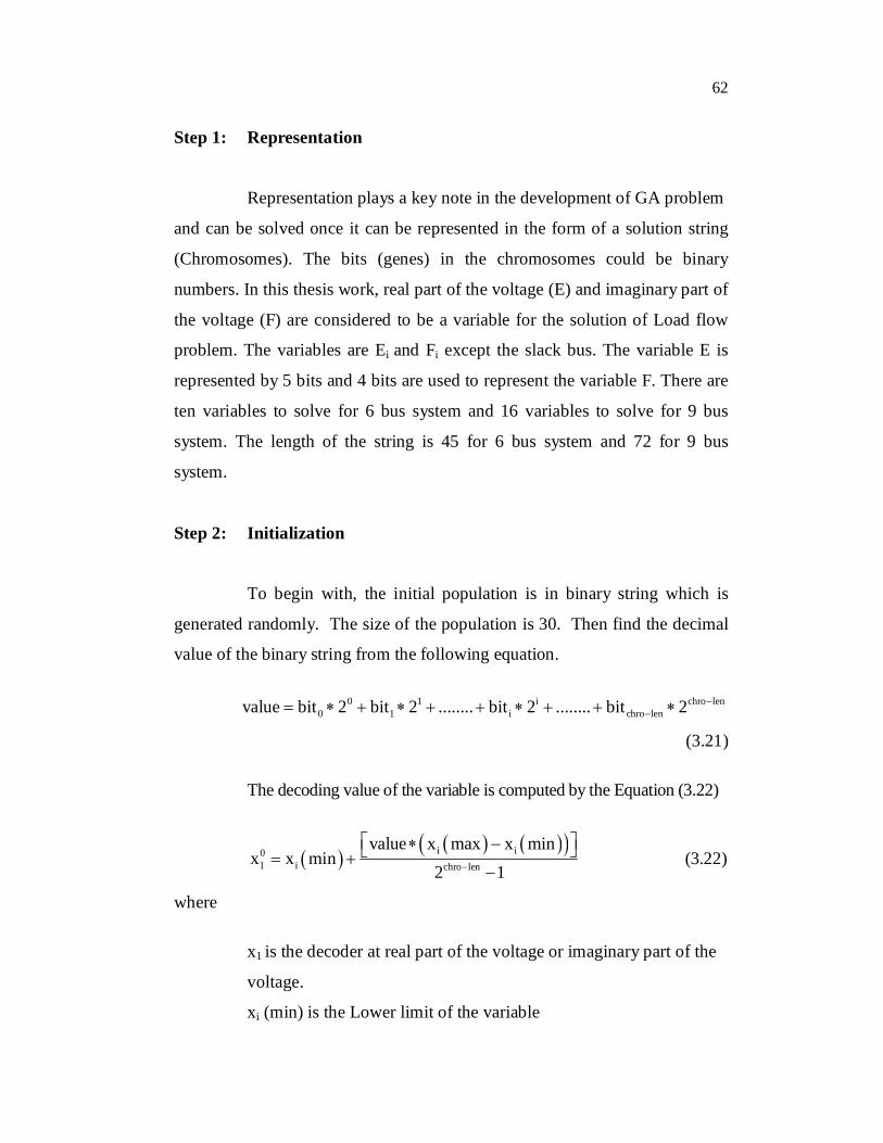
Step 1: Representation

Representation plays a key note in the development of GA problem

and can be solved once it can be represented in the form of a solution string

(Chromosomes). The bits (genes) in the chromosomes could be binary

numbers. In this thesis work, real part of the voltage (E) and imaginary part of

the voltage (F) are considered to be a variable for the solution of Load flow

problem. The variables are Ei and Fi except the slack bus. The variable E is

represented by 5 bits and 4 bits are used to represent the variable F. There are

ten variables to solve for 6 bus system and 16 variables to solve for 9 bus

system. The length of the string is 45 for 6 bus system and 72 for 9 bus

system.

Step 2: Initialization

To begin with, the initial population is in binary string which is

generated randomly. The size of the population is 30. Then find the decimal

value of the binary string from the following equation.

0 1 i chro len0 1 i chro lenvalue bit 2 bit 2 ........ bit 2 ........ bit 2

(3.21)

The decoding value of the variable is computed by the Equation (3.22)

i i0

1 i chro len

value x max x minx x min

2 1

(3.22)

where

x1 is the decoder at real part of the voltage or imaginary part of the

voltage.

xi (min) is the Lower limit of the variable

63

xi (max) is the Upper limit of the variable

chro-len is the Total length of the string

value is the decimal value equivalent to the binary string.

In this thesis work, on the PQ nodes, the variables were specified in

the intervals (0.9, 1.0) for E and (-0.2, 0.2) for F. The variation for E and F on

PV nodes were specified in the intervals (0.9, 1.1) and (-0.3, 0.3)

Step 3: Calculation of fitness value

The fitness function for each variable is determined by finding the

value of objective function to that variable, which is given below:

Fitness function 2loss

1f (E,F)1 g(E,F) WP

(3.23)

The fitness function is computed for every individual of the

population. In the maximation problem, the string which has higher fitness

value will be the best string.

Step 4: Selection or reproduction

Reproduction selects good strings in a population and forms a

mating pool. Reproduction operator is also called as selection operator. In this

work, tournament selection is used.

Step 5: Cross Over

Cross Over is a mechanism for diversification. The strings to be

crossed and the crossing points are selected randomly and crossover is done

64

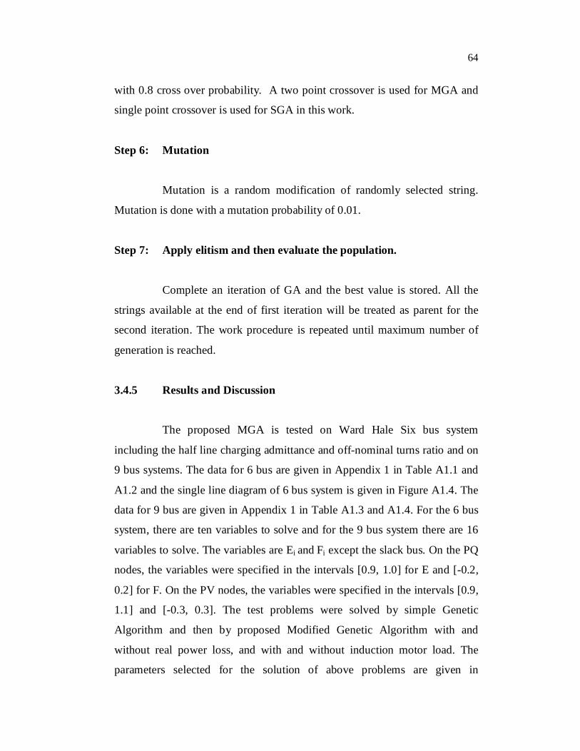
with 0.8 cross over probability. A two point crossover is used for MGA and

single point crossover is used for SGA in this work.

Step 6: Mutation

Mutation is a random modification of randomly selected string.

Mutation is done with a mutation probability of 0.01.

Step 7: Apply elitism and then evaluate the population.

Complete an iteration of GA and the best value is stored. All the

strings available at the end of first iteration will be treated as parent for the

second iteration. The work procedure is repeated until maximum number of

generation is reached.

3.4.5 Results and Discussion

The proposed MGA is tested on Ward Hale Six bus system

including the half line charging admittance and off-nominal turns ratio and on

9 bus systems. The data for 6 bus are given in Appendix 1 in Table A1.1 and

A1.2 and the single line diagram of 6 bus system is given in Figure A1.4. The

data for 9 bus are given in Appendix 1 in Table A1.3 and A1.4. For the 6 bus

system, there are ten variables to solve and for the 9 bus system there are 16

variables to solve. The variables are Ei and Fi except the slack bus. On the PQ

nodes, the variables were specified in the intervals [0.9, 1.0] for E and [-0.2,

0.2] for F. On the PV nodes, the variables were specified in the intervals [0.9,

1.1] and [-0.3, 0.3]. The test problems were solved by simple Genetic

Algorithm and then by proposed Modified Genetic Algorithm with and

without real power loss, and with and without induction motor load. The

parameters selected for the solution of above problems are given in

65

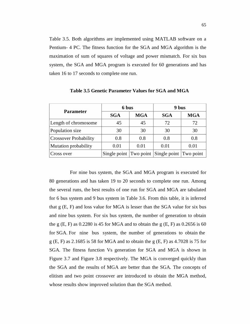
Table 3.5. Both algorithms are implemented using MATLAB software on a

Pentium- 4 PC. The fitness function for the SGA and MGA algorithm is the

maximation of sum of squares of voltage and power mismatch. For six bus

system, the SGA and MGA program is executed for 60 generations and has

taken 16 to 17 seconds to complete one run.

Table 3.5 Genetic Parameter Values for SGA and MGA

Parameter 6 bus 9 bus

SGA MGA SGA MGA Length of chromosome 45 45 72 72 Population size 30 30 30 30 Crossover Probability 0.8 0.8 0.8 0.8 Mutation probability 0.01 0.01 0.01 0.01 Cross over Single point Two point Single point Two point

For nine bus system, the SGA and MGA program is executed for

80 generations and has taken 19 to 20 seconds to complete one run. Among

the several runs, the best results of one run for SGA and MGA are tabulated

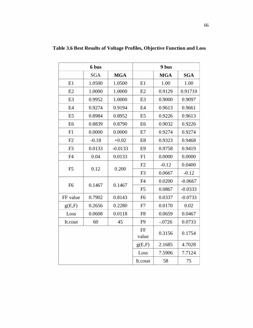
for 6 bus system and 9 bus system in Table 3.6. From this table, it is inferred

that g (E, F) and loss value for MGA is lesser than the SGA value for six bus

and nine bus system. For six bus system, the number of generation to obtain

the g (E, F) as 0.2280 is 45 for MGA and to obtain the g (E, F) as 0.2656 is 60

for SGA. For nine bus system, the number of generations to obtain the

g (E, F) as 2.1685 is 58 for MGA and to obtain the g (E, F) as 4.7028 is 75 for

SGA. The fitness function Vs generation for SGA and MGA is shown in

Figure 3.7 and Figure 3.8 respectively. The MGA is converged quickly than

the SGA and the results of MGA are better than the SGA. The concepts of

elitism and two point crossover are introduced to obtain the MGA method,

whose results show improved solution than the SGA method.

66

Table 3.6 Best Results of Voltage Profiles, Objective Function and Loss

6 bus 9 bus SGA MGA MGA SGA

E1 1.0500 1.0500 E1 1.00 1.00 E2 1.0000 1.0000 E2 0.9129 0.91710 E3 0.9952 1.0000 E3 0.9000 0.9097 E4 0.9274 0.9194 E4 0.9613 0.9661 E5 0.8984 0.8952 E5 0.9226 0.9613 E6 0.8839 0.8790 E6 0.9032 0.9226 F1 0.0000 0.0000 E7 0.9274 0.9274 F2 -0.18 +0.02 E8 0.9323 0.9468 F3 0.0133 -0.0133 E9 0.9758 0.9419 F4 0.04 0.0133 F1 0.0000 0.0000

F5 0.12 0.200 F2 -0.12 0.0400 F3 0.0667 -0.12

F6 0.1467 0.1467 F4 0.0200 -0.0667 F5 0.0867 -0.0333

FF value 0.7902 0.8143 F6 0.0337 -0.0733 g(E,F) 0.2656 0.2280 F7 0.0170 0.02 Loss 0.0608 0.0118 F8 0.0659 0.0467

It.cout 60 45 F9 -.0726 0.0733

FF value 0.3156 0.1754

g(E,F) 2.1685 4.7028 Loss 7.5906 7.7124

It.coun 58 75

67

o b j. f u n c v s g e n e r a t i o n ( fo r 6 b u s s y s t e m )

00 . 10 . 20 . 30 . 40 . 50 . 60 . 70 . 80 . 9

1 6 1 1 1 6 2 1 2 6 3 1 3 6 4 1 4 6 5 1 5 6

g e n e r a t i o n

obj.f

un.

M G A

S G A

Figure 3.7 Objective Function Vs Generation for Six Bus System

O b j .F u n c .V s g e n e r a t io n( f o r 9 b u s s y s t e m )

00 . 0 5

0 . 10 . 1 5

0 . 20 . 2 5

0 . 30 . 3 5

1 6 1 1 1 6 2 1 2 6 3 1 3 6 4 1 4 6 5 1 5 6 6 1 6 6 7 1 7 6

g e n e r a t i o n

obj.f

unc

S G A

M G A

Figure 3.8 Objective Function Vs Generation for Nine Bus System

Four cases have been studied. Case ‘a’ describes the best results for

the objective function of sum of squares of voltage and power mismatch using

MGA. Case ‘b’ describes the best results when the real power loss is added as

a constraint to the Case ‘a’ using MGA. Case ‘c’ describes the best results

when the Induction motor is added to the case ‘a’ using MGA. Case ‘d’

describes the best results when the Induction motor and real power loses is

considered. The induction motor is added to the sixth bus for Ward Hale 6 bus

system and to the ninth bus for 9 bus system in addition to the PQ bus. The

obj.func. Vs generation (for 6 bus system)

obj.func. Vs generation (for 9 bus system)

68

results of case ‘a’, case ‘b’, case ‘c’ and case ‘d’ are tabulated in Table 3.7

and Table 3.8 for 6 bus system and 9 bus system respectively. By comparing

the results of case ‘b’ with the case ‘a’ it can be inferred that the voltage

profiles are improved but the objective function value is decreased. Next the

results of case ‘c’ are compared with case ‘a’ results. There is an increase in

the voltage profiles but the objective function value is lesser than case ‘a’

value but greater than case ‘b’ value. So the iteration count lies between Case

‘a’ and case ‘b’. Finally the result of case ‘d’ are compared with case ‘a’. Here

the voltage profiles are further improved and the objective function value lies

between the case ‘b’ and case ‘c’. So the iteration count is less than case ‘a’

but greater than case ‘b’ and case ‘c’. The voltage profiles versus bus number

for case ‘a’, case ‘b’, case ‘c’ and case ‘d’ for 6 and 9 bus systems are shown

in Figure 3.9 and Figure 3.10 respectively.

Table 3.7 Best Results for case a, case b, case c and case d of Six Bus System

(W=50)

case a case b case c case d It. count 45 32 30 38 Obj. fun. 0.8143 0.7730 0.5391 0.5748 g(E,F) 0.2281 0.2868 0.8549 0.5644 PLOSS 0.0163 0.0118 0.0996 0.0542 V2 1.0000 1.0194 1.0003 1.0516 V3 1.0000 1.0000 0.8710 0.9597 V4 0.9194 0.9290 0.8065 0.8710 V5 0.8952 0.9290 0.9355 0.9435 V6 0.8790 0.9032 0.75 0.7500 F2 0.02 0.02 -0.3 -0.3000 F3 -0.0133 -0.0933 -0.1497 -0.2000 F4 0.0133 -0.04 -0.0933 -0.1200 F5 0.2000 0.1733 -0.0933 -0.1200 F6 0.1467 0.12 -0.04 -0.0400

69

Table 3.8 Best Results for case a, case b, case c and case d of Nine Bus System

(W=0.1)

Case a Case b Case c Case d

It count 58 56 51 48

Obj. fun 0.3156 0.1051 0.3095 0.0955

g(E,F) 2.1685 2.4125 2.2312 3.1790

PLOSS 7.5906 7.8106 8.3192 7..9355

V2 0.9129 0.9758 1.0000 10194

V3 0.9000 0.9516 0.9903 0.9516

V4 0.9613 0.9661 0.9806 0.9716

V5 0.9226 0.9129 0.9710 0.9226

V6 0.9032 0.9371 0.9855 0.9468

V7 0.9274 0.9371 09661 0.9565

V8 0.9323 0.9710 0.9855 0.9661

V9 0.9758 0.9758 0.9758 0.9758

F2 -0.1200 -0.1800 0.0600 -0.2600

F3 0.0667 0.1000 0.1000 0.1000

F4 0.0200 0.0400 0.0400 0.0400

F5 0.0867 0.0933 0.0933 0.0933

F6 0.0733 0.1200 0.1467 0.1200

F7 0.0467 0.0667 0.1733 0.0400

F8 -0.0333 -0.04 0.1200 -0.0933

F9 0.0463 0.0667 0.0933 0.0667

70

V o l t a g e p r o f i l e s V s B u s n o . ( f o r 6 b u s s y s t e m )

0

0 . 2

0 . 4

0 . 6

0 . 8

1

1 . 2

1 2 3 4 5 6

b u s n o .

real

vol

tage

(p.u

)C a s e b

C a s e c

C a s e dC a s e a

Figure 3.9 Real Voltage Profiles Vs Bus Number for Six Bus System

V o lt a g e p r o f i le s V s B u s n o .( f o r 9 b u s s y s t e m )

0 . 8 40 . 8 60 . 8 8

0 . 90 . 9 20 . 9 40 . 9 60 . 9 8

11 . 0 2

1 2 3 4 5 6 7 8

b u s n o .

real

vol

tage

(p.u

)

C a s e a

C a s e b

C a s e c

C a s e d

Figure 3.10 Real Voltage Profiles Vs Bus Number for Nine bus System

From the above discussion, the losses added to the power and

voltage mismatches will cause the increase in voltage profiles and decrease

the iteration count. The addition of induction motor to the PQ load bus also

improves the performance and also reduces the iteration count. The addition

of induction motor and real power loss to the voltage and power mismatches

gives better voltage profiles even though the objective function is less when

compared to the case ‘a’.

71

3.5 CONCLUSION

Review of GA and the difference between other traditional

optimization methods have been presented in this chapter. The advantages of

FSGA, MGA over simple GA were also discussed. In this chapter, FSGA

based solution for the load flow problem has been presented. Without any

requirements for auxiliary information and calculation of derivatives, a simple

and efficient algorithm is proposed. In this research work, basic genetic

operators like reproduction, crossover, mutation and advanced operators like

hill climbing were discussed. The results of SGA and the proposed method

FSGA were compared with NR method. FSGA gives better voltage profiles

than the NR and SGA method. The advanced operators of FSGA like Elitism

and Hill climbing leads to the less computation time and an improved solution

to the six bus system. It can be easily coded to work on parallel computers.

This chapter has also presented a MGA based solution for the load

flow problems with Induction motor and real power loss. In this research

work, basic genetic operators and improved operators like Elitism and two

point crossover were discussed. The results of SGA and the proposed MGA

were compared. Computer processing time to execute the SGA and MGA

program for the maximum number of generation is nearly same. The Elitism

concept of MGA leads to quick convergence and an improved solution.

Finally the results of case ‘a’, case ‘b’, case ‘c’ and case ‘d’ were compared.

The addition of real power loss and the non linear load will give the precise

voltage profiles and also speedup the convergence.