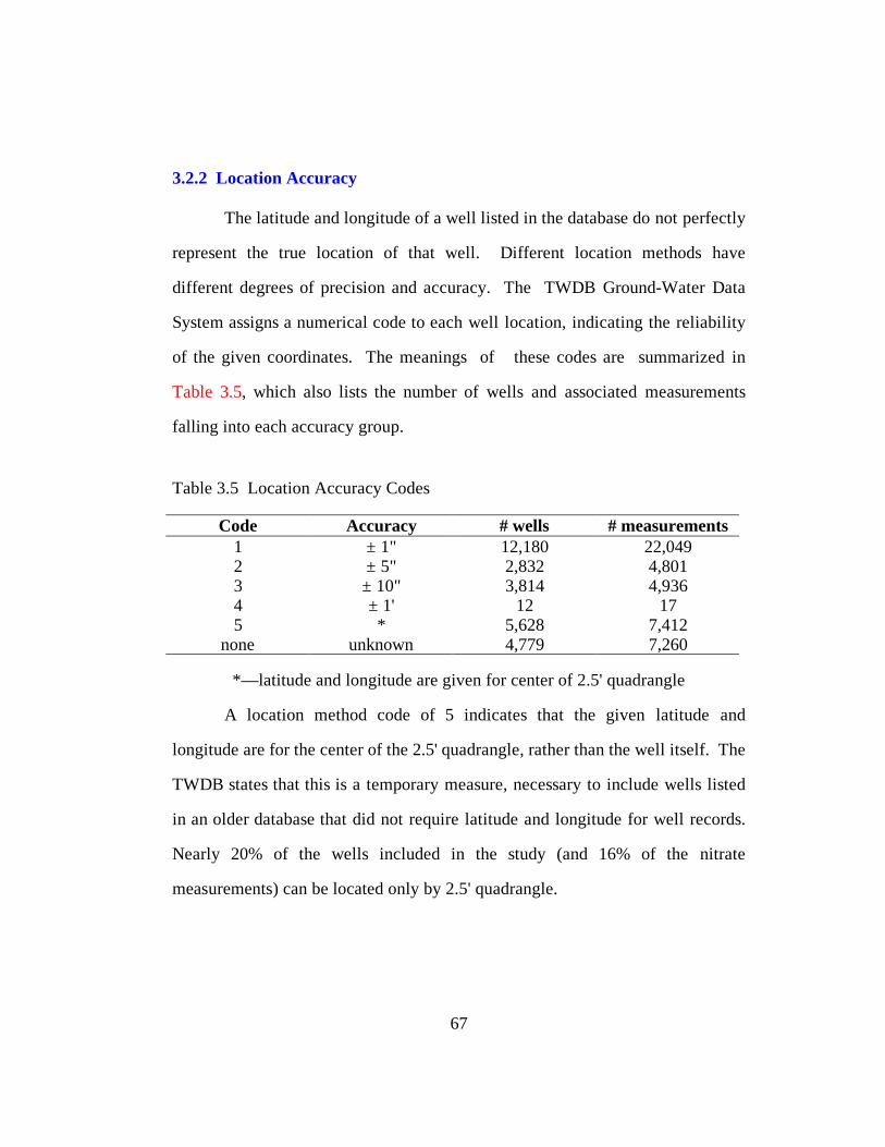
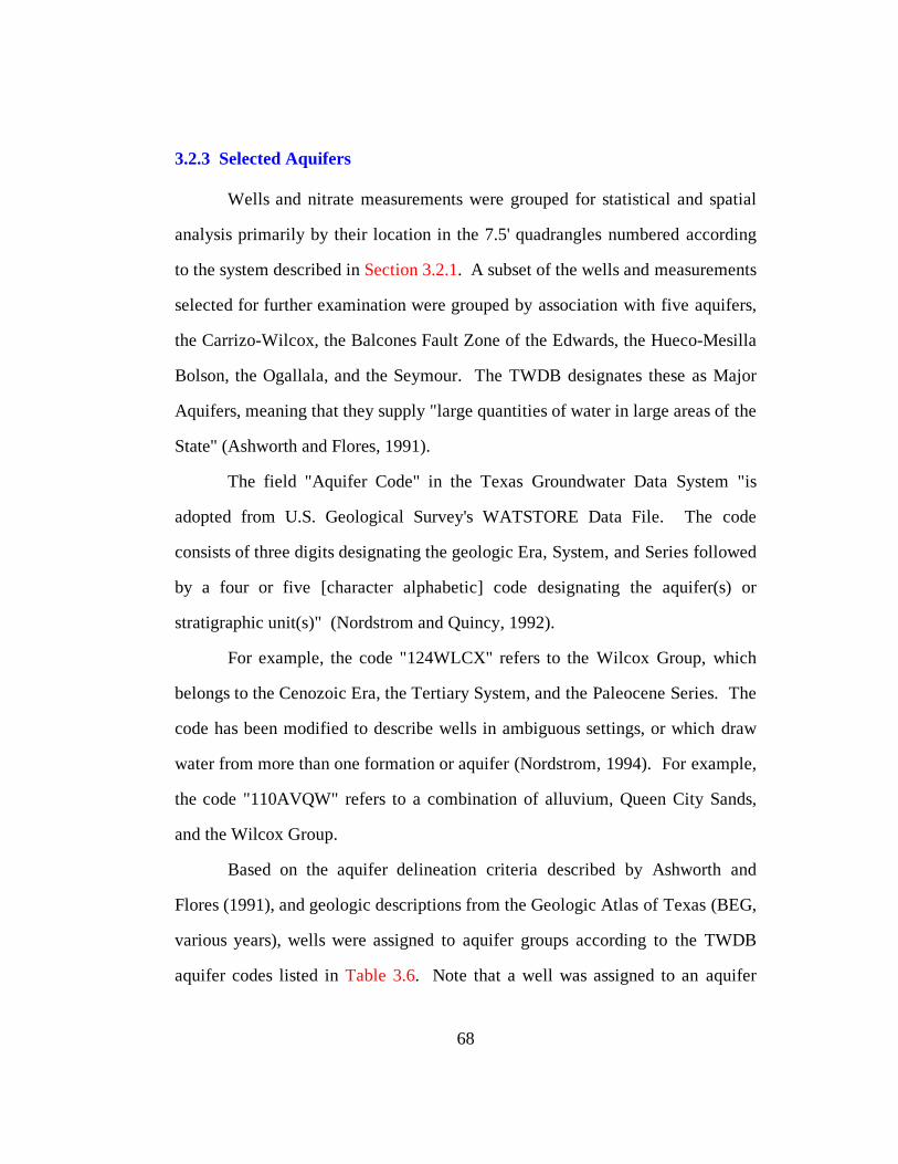
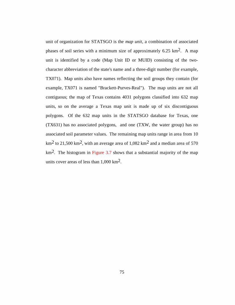
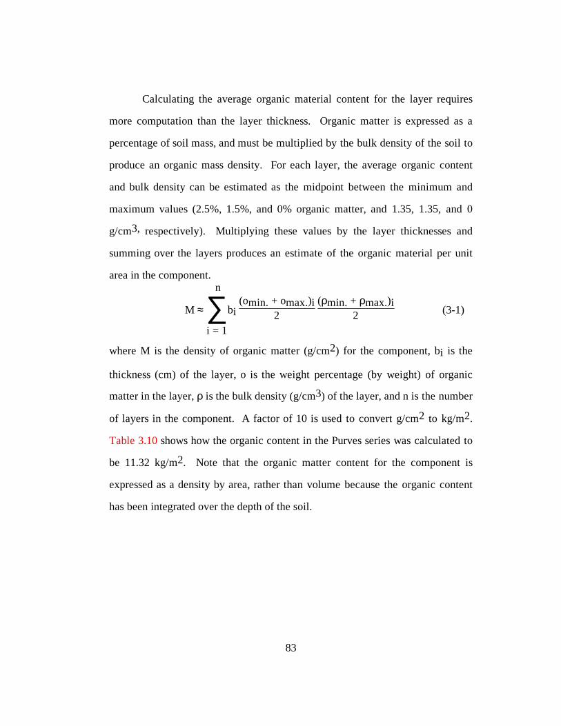
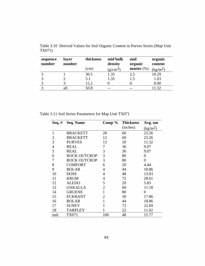
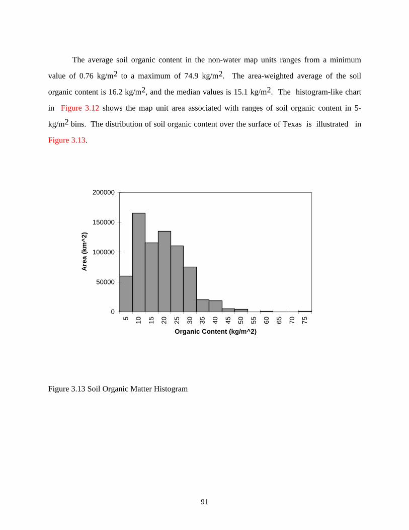
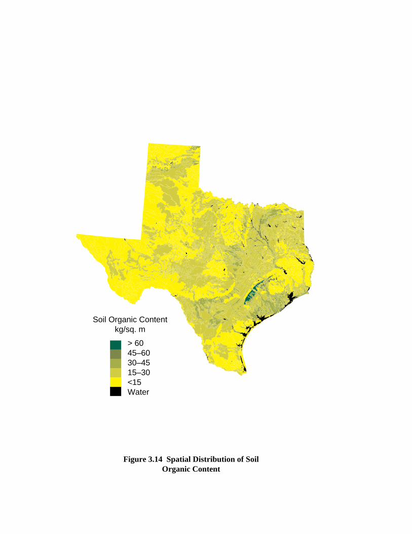
55 Chapter 3: Data Sources and Description The conclusions that this study presents are based on statistics calculated from 46,507 nitrate measurements taken from 29,485 wells throughout Texas. Following the methods outlined in Section 2.6, and described in detail in Chapter4, the spatial variation of the statistics is mapped to identify regions of high or low vulnerability to nitrate contamination. The spatial variation in the statistics is then compared to the spatial variation of potential water quality indicators, including soil parameters, average annual precipitation, and fertilizer sales, in order to assess the value of these data as indicators of water quality. Because the structure and limitations of these data strongly influence the choice of the methods used, this chapter, which describes the data itself, is a necessary prelude to Chapters 4 and 5, which describe the methodology and procedures followed in the study. This chapter contains seven sections, one for each data set used in the study. These data sets can be divided into three groups: 1) Primary data, consisting of groundwater nitrate concentration measurements and descriptions of the wells where the groundwater was collected for testing. The nitrate data are described in Section 3.1 and the well data are described in Section 3.2. 2) Data to be considered as potential indicators of water quality. These include soil thickness and organic content described in Section 3.3; annual average precipitation, described in Section 3.4; and average annual nitrogen fertilizer sales, described in Section 3.5.
Transcript
55
Chapter 3: Data Sources and Description
The conclusions that this study presents are based on statistics calculated
from 46,507 nitrate measurements taken from 29,485 wells throughout Texas.
Following the methods outlined in Section 2.6, and described in detail in
Chapter4, the spatial variation of the statistics is mapped to identify regions of
high or low vulnerability to nitrate contamination. The spatial variation in the
statistics is then compared to the spatial variation of potential water quality
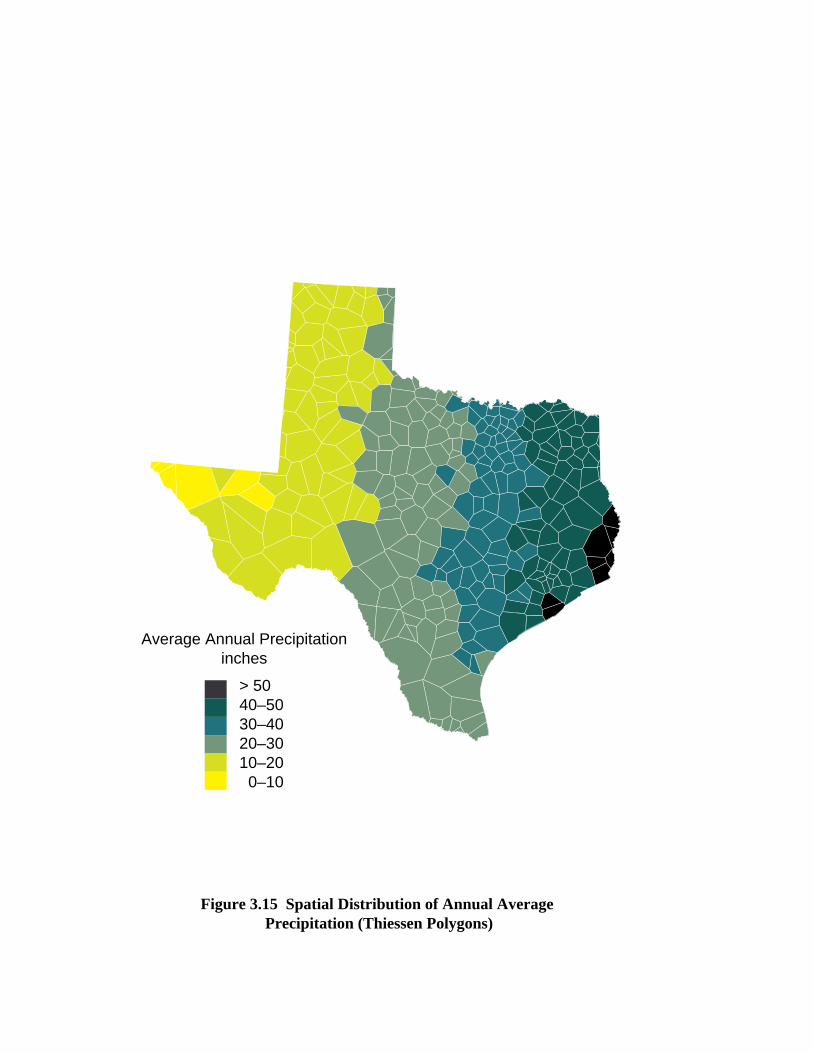
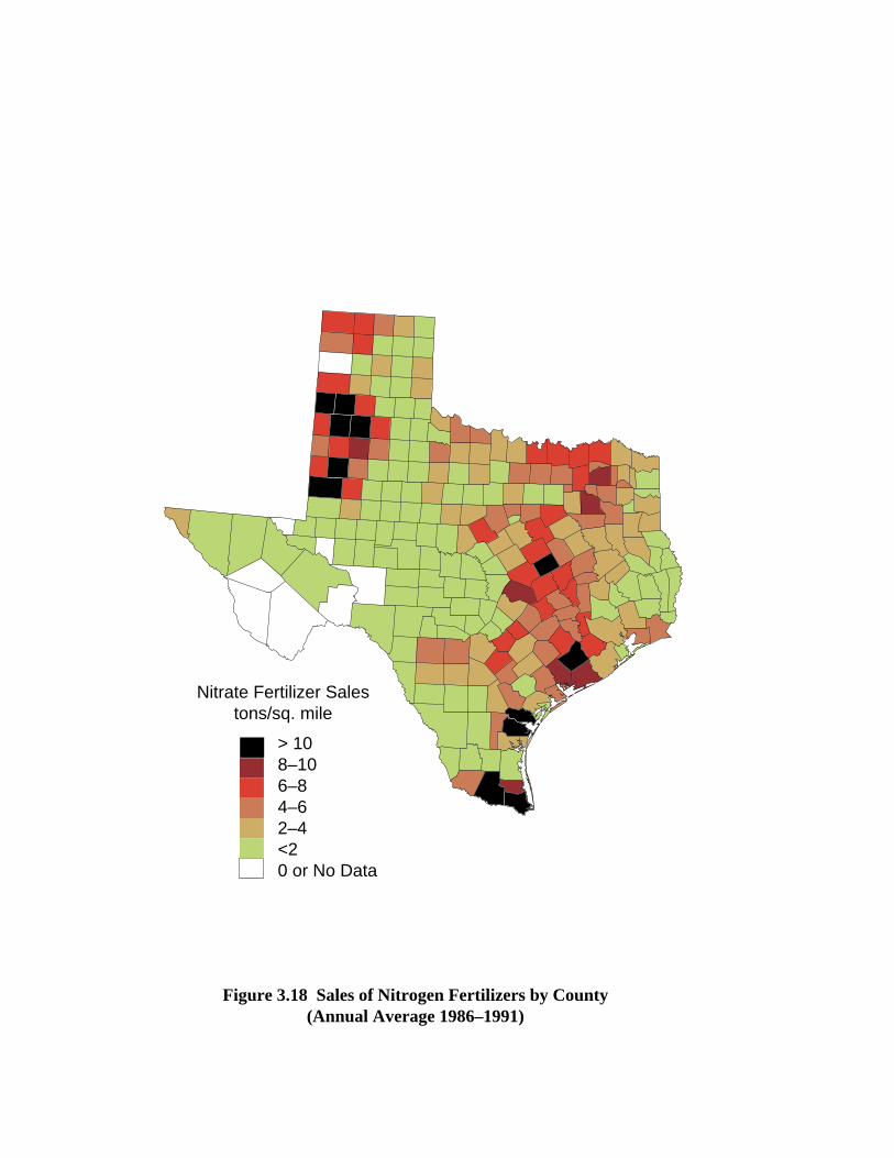
indicators, including soil parameters, average annual precipitation, and fertilizer
sales, in order to assess the value of these data as indicators of water quality.
Because the structure and limitations of these data strongly influence the
choice of the methods used, this chapter, which describes the data itself, is a
necessary prelude to Chapters 4 and 5, which describe the methodology and
procedures followed in the study. This chapter contains seven sections, one for
each data set used in the study. These data sets can be divided into three groups:
1) Primary data, consisting of groundwater nitrate concentration measurements
and descriptions of the wells where the groundwater was collected for
testing. The nitrate data are described in Section 3.1 and the well data are
described in Section 3.2.
2) Data to be considered as potential indicators of water quality. These include
soil thickness and organic content described in Section 3.3; annual
average precipitation, described in Section 3.4; and average annual
nitrogen fertilizer sales, described in Section 3.5.
56
3) Independent measurements of nitrate and herbicides, used to test assumptions
made in the study. These include measurements of nitrate in public water
sources collected by the Water Utilities Division of the Texas Natural
Resource Conservation Commission, described in Section 3.6, and the
first year's results of the U.S. Geological Survey's reconnaissance of
nitrate and herbicides in groundwater in the Midwest, described in
Section 3.7.
3.1 NITRATE MEASUREMENT DATA
The nitrate measurements used in this study come from the Texas Water
Development Board's (TWDB) Groundwater Data System (Nordstrom and
Quincy, 1992). This statewide database contains physical descriptions of wells
and their surroundings in Texas, and levels of chemical constituents measured by
a variety of public agencies. The TWDB maintains the database to characterize
the quantity and quality of groundwater available throughout the state, in support
of the preparation of the Texas Water Plan (TWDB, 1994).
For every nitrate measurement listed in the Groundwater Data System as
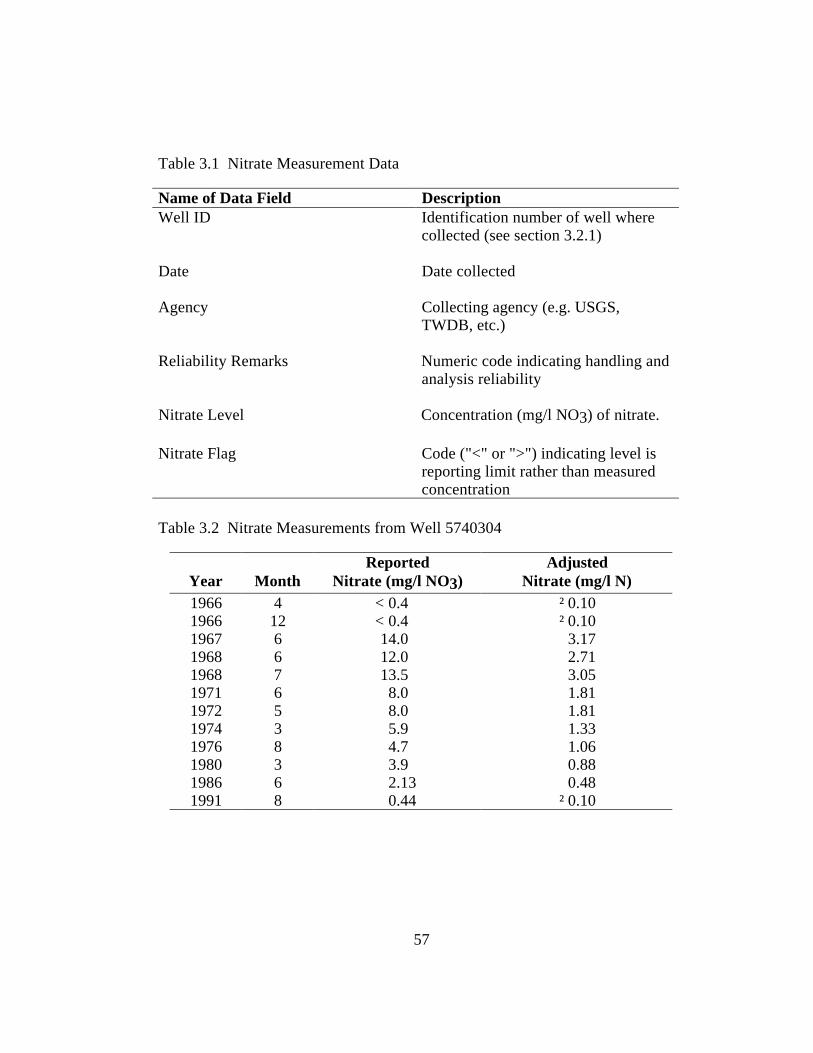
of October 1993—a total of 62,692 database records—the data fields listed in
Table 3.1 were retrieved for use in this study. Of these data fields, the well ID,
date, and nitrate level have values in all records. Many records have no values
for the collecting agency or reliability remarks. The values in the flag field are
discussed in section 3.1.1.
57
Table 3.1 Nitrate Measurement Data
Well ID Identification number of well wherecollected (see section 3.2.1)
Nitrate concentrations in the TWDB database are listed as mg/l nitrate
(nitrate-NO3). However, unless otherwise noted the values used in this study's
statistical analyses and reported here are in equivalent values of nitrate as
nitrogen (nitrate-N), the units used in EPA regulations. 1 mg/l nitrate-N equals
4.42 mg/l nitrate-NO3. Each nitrate-NO3 value in the data set was converted to
an equivalent nitrate-N value. To maintain a uniform reporting limit for all
records used in the study, all values at or below a value of 0.1 mg/l nitrate-N will
be treated as ² 0.1 mg/l. A nitrate concentration greater than 0.1 mg/l will be
considered a "detection" and concentrations less than or equal to this value will
be considered to be "below detection limit." As an illustration of this conversion
and adjustment, Table 3.2 shows the nitrate measurements listed in the TWDB
database for well 5740304 and the adjusted values used for analysis in this study.
Of the twelve measurements shown, nine are considered detections of nitrate and
three fall below the detection limit.
3.1.1 Nitrate Reporting Limits
The flag field in a nitrate measurement record may be blank or may
contain a "<" or ">" character. A blank should indicate that the value listed for
nitrate concentration in the nitrate level field is the actual value measured in the
water; a "<" or ">" indicates that the value is a detection or reporting limit,
rather than an actual value. The ">" character appeared 5 times in the retrieved
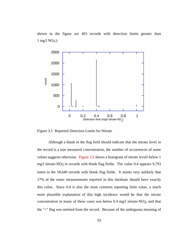
data. The "<" character appears in 4047 (6.5%) of the records. A value of 0.40
mg/l nitrate-NO3 (approximately equal to 0.1 mg/l nitrate-N) appears most
frequently as a reporting limit, as the histogram in Figure 3.1 illustrates. (Not
59
shown in the figure are 403 records with detection limits greater than
1 mg/l NO3.)
0
500
1000
1500
2000
2500
0 0.2 0.4 0.6 0.8 1
coun
t
Detection limit (mg/l nitrate-NO3)
Figure 3.1 Reported Detection Limits for Nitrate
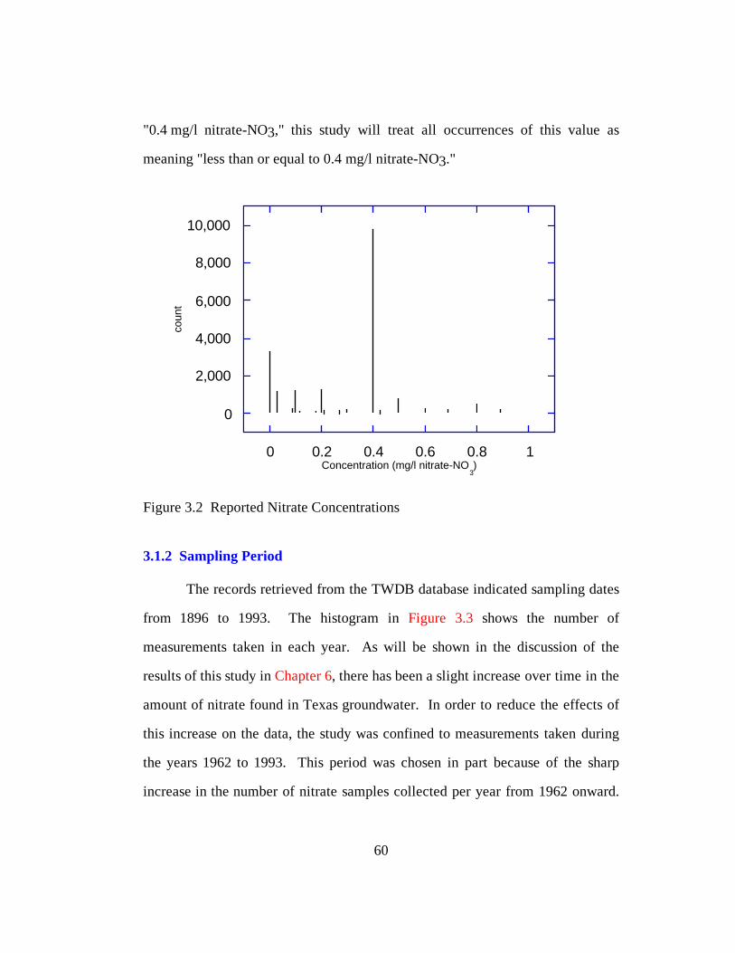
Although a blank in the flag field should indicate that the nitrate level in
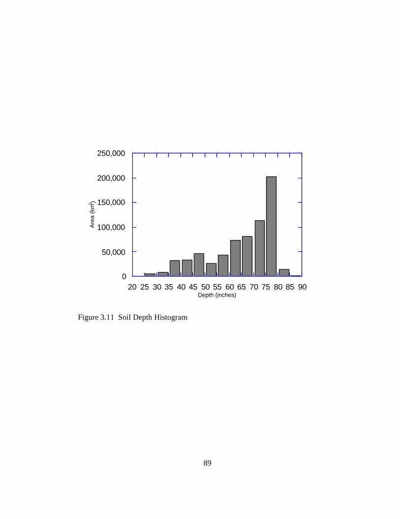
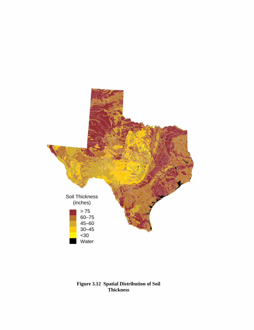
the record is a true measured concentration, the number of occurrences of some
values suggests otherwise. Figure 3.2 shows a histogram of nitrate levels below 1
mg/l nitrate-NO3 in records with blank flag fields. The value 0.4 appears 9,793
times in the 58,640 records with blank flag fields. It seems very unlikely that
17% of the water measurements reported in this database should have exactly
this value. Since 0.4 is also the most common reporting limit value, a much
more plausible explanation of this high incidence would be that the nitrate
concentration in many of these cases was below 0.4 mg/l nitrate-NO3, and that
the "<" flag was omitted from the record. Because of the ambiguous meaning of
60
"0.4 mg/l nitrate-NO3," this study will treat all occurrences of this value as
meaning "less than or equal to 0.4 mg/l nitrate-NO3."
0
2,000
4,000
6,000
8,000
10,000
0 0.2 0.4 0.6 0.8 1
coun
t
Concentration (mg/l nitrate-NO3)
Figure 3.2 Reported Nitrate Concentrations
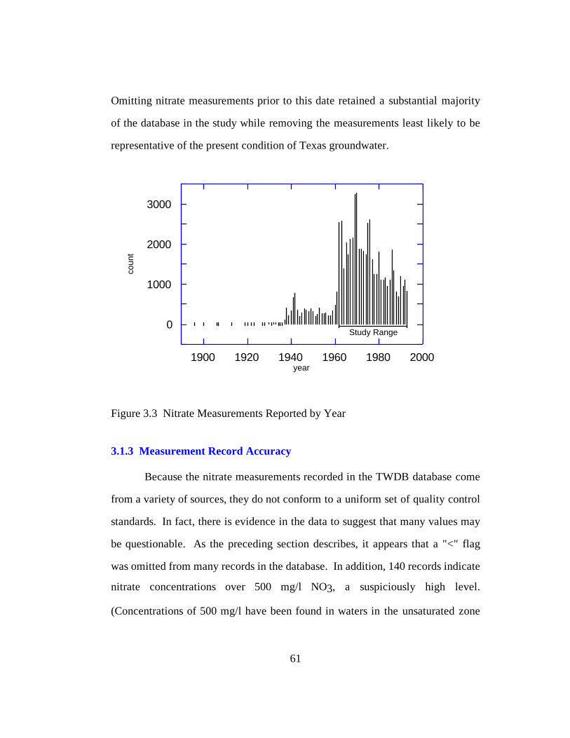
3.1.2 Sampling Period
The records retrieved from the TWDB database indicated sampling dates
from 1896 to 1993. The histogram in Figure 3.3 shows the number of
measurements taken in each year. As will be shown in the discussion of the
results of this study in Chapter 6, there has been a slight increase over time in the
amount of nitrate found in Texas groundwater. In order to reduce the effects of
this increase on the data, the study was confined to measurements taken during
the years 1962 to 1993. This period was chosen in part because of the sharp
increase in the number of nitrate samples collected per year from 1962 onward.
61
Omitting nitrate measurements prior to this date retained a substantial majority
of the database in the study while removing the measurements least likely to be
representative of the present condition of Texas groundwater.
0
1000
2000
3000
1900 1920 1940 1960 1980 2000
coun
t
year
Study Range
Figure 3.3 Nitrate Measurements Reported by Year
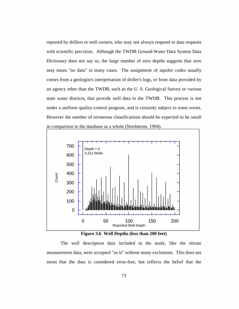
3.1.3 Measurement Record Accuracy
Because the nitrate measurements recorded in the TWDB database come
from a variety of sources, they do not conform to a uniform set of quality control
standards. In fact, there is evidence in the data to suggest that many values may
be questionable. As the preceding section describes, it appears that a "<" flag
was omitted from many records in the database. In addition, 140 records indicate
nitrate concentrations over 500 mg/l NO3, a suspiciously high level.
(Concentrations of 500 mg/l have been found in waters in the unsaturated zone
62
below irrigated crops, and levels over 1000 mg/l have been found in pools in the
parts of Carlsbad Caverns where bats roost (Hem, 1989). It seems unlikely that
concentrations this high are representative of natural groundwater.) 51,329 of
the 62,692 nitrate records retrieved from the TWDB database had blank
reliability remark fields; while this provides no grounds for excluding the
records, it is not a ringing endorsement either.
In spite of these reservations, this study has taken an "innocent until
proven guilty" approach to the measurement records. The data were included in
the study "as is" unless substantial evidence indicated that they should be
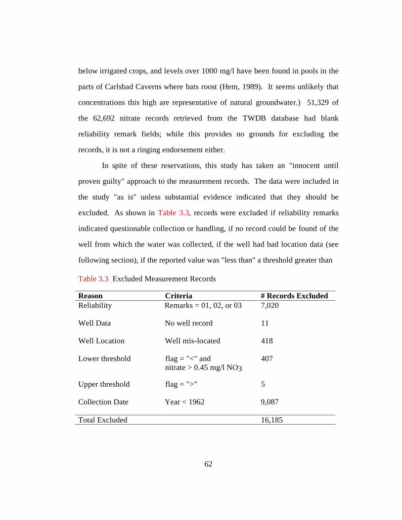
excluded. As shown in Table 3.3, records were excluded if reliability remarks
indicated questionable collection or handling, if no record could be found of the
well from which the water was collected, if the well had bad location data (see
following section), if the reported value was "less than" a threshold greater than
Table 3.3 Excluded Measurement Records
Reason Criteria # Records ExcludedReliability Remarks = 01, 02, or 03 7,020
Well Data No well record 11
Well Location Well mis-located 418
Lower threshold flag = "<" andnitrate > 0.45 mg/l NO3
407
Upper threshold flag = ">" 5
Collection Date Year < 1962 9,087
Total Excluded 16,185
63
0.1 mg/l nitrate-N (0.45 mg/l NO3), if the reported value was "greater than" any
threshold, or if the measurement was taken before 1962 (see preceding section).
These exclusions left 46,507 nitrate measurement records in the study. This set
of nitrate measurement records will be called the "base data set" in the remainder
of this document.
3.2 WELL DATA
The data providing physical descriptions of the wells included in the
study comes from the same TWDB database as the nitrate measurement data.
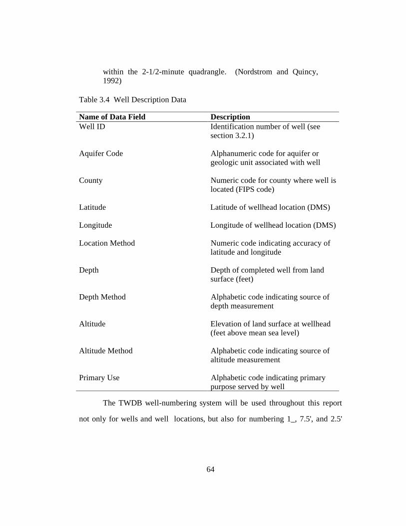
For each well for which a nitrate measurement was recorded—a total of 38,740
database records—the data fields listed in Table 3.4 were retrieved.
3.2.1 TWDB Well Numbers
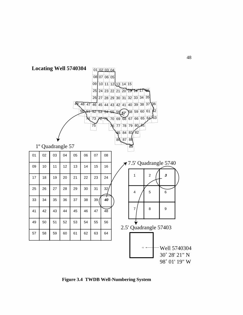
TWDB has adopted a system of identification numbers for wells in Texas,
based on the location of the wells expressed in latitude and longitude. The
following description and Figure 3.4 explain the numbering system.
[The numbering system] is based on division of the state into agrid of 1-degree quadrangles formed by degrees of latitude andlongitude and the repeated division of these quadrangles intosmaller ones as shown…
Each 1-degree quadrangle is divided into sixty-four 7-1/2-minutequadrangles, each of which is further divided into nine 2-1/2-minute quadrangles. Each 1-degree quadrangle in the state hasbeen assigned an identification number. The 7-1/2-minutequadrangles are numbered consecutively from left to right,beginning in the upper-left-hand corner of the 1-degreequadrangle, and the 2-1/2-minute quadrangles within each 7-1/2-minute quadrangle are similarly numbered. The first 2 digits of awell number identify the 1-degree quadrangle; the third and fourthdigits, the 7-1/2-minute quadrangle; the fifth digit identifies the 2-1/2-minute quadrangle; and the last two digits identify the well
64
within the 2-1/2-minute quadrangle. (Nordstrom and Quincy,1992)
Table 3.4 Well Description Data
Well ID Identification number of well (seesection 3.2.1)
Aquifer Code Alphanumeric code for aquifer orgeologic unit associated with well
County Numeric code for county where well islocated (FIPS code)
Latitude Latitude of wellhead location (DMS)
Longitude Longitude of wellhead location (DMS)
Location Method Numeric code indicating accuracy oflatitude and longitude
Depth Depth of completed well from landsurface (feet)