Chapter 3 Experimental Techniques Stress measurements using optical bending beam method can be applied for UHV sys- tem as well as in air. However, the magnetic properties of ultra thin films are better to be measured in-situ as deposited, as the magnetic properties can be sensitive to the surface conditions. The surface changes such as adsorption or desorption processes can only be studied in a UHV environment. Hence the measurements are all performed in a UHV system, the relative techniques and the UHV apparatus are introduced in this chapter. 3.1 Optical bending beam method The stress measurements in this work are carried out using the optical bending beam method based on the cantilever technique. The idea of stress measurement using can- tilever bending originates from the pioneering work by Stoney [59], who related the curvature of the sample with film stress. Today the advanced techniques measure the curvature of the sample by detecting the capacitance [28] or the optical deflec- tion [60,61], which greatly increased the sensitivity so that small surface stress changes can also be measured. Similar optical method have been successfully employed in sur- face stress and film stress measurements for Si samples [62, 63]. The principle of the technique is shown in Figure 3.1(b). The rectangular thin substrate is clamped along its width at the upper end and free at the lower end. It is used as a cantilever that will bend when its front side and backside endure different forces or stresses. A laser beam is used to detect the deflection of the cantilever sample. The laser beam is split in two beams that are aligned to point at the sample surface with a short separation in between. Subsequently, the beams reflected from the surface are detected by two separated position-sensitive detectors with photo current amplifier that transform the positions of the beams into voltages. The position changes (Δd) of the two laser beams on the detectors are transferred into the slope changes Δm on the sample surface where they are reflected: Δm = Δd 2L in which L is the distance between the sample and the detector. The curvature of the substrate κ =1/R can be obtained from the slope differences and the separation
Transcript
Chapter 3
Experimental Techniques
Stress measurements using optical bending beam method can be applied for UHV sys-tem as well as in air. However, the magnetic properties of ultra thin films are betterto be measured in-situ as deposited, as the magnetic properties can be sensitive to thesurface conditions. The surface changes such as adsorption or desorption processes canonly be studied in a UHV environment. Hence the measurements are all performed ina UHV system, the relative techniques and the UHV apparatus are introduced in thischapter.
3.1 Optical bending beam method
The stress measurements in this work are carried out using the optical bending beammethod based on the cantilever technique. The idea of stress measurement using can-tilever bending originates from the pioneering work by Stoney [59], who related thecurvature of the sample with film stress. Today the advanced techniques measurethe curvature of the sample by detecting the capacitance [28] or the optical deflec-tion [60,61], which greatly increased the sensitivity so that small surface stress changescan also be measured. Similar optical method have been successfully employed in sur-face stress and film stress measurements for Si samples [62,63].
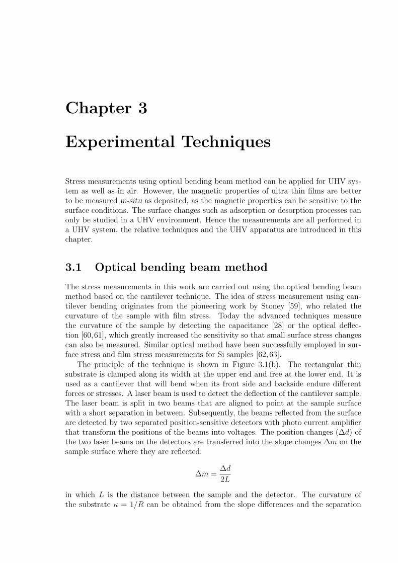
The principle of the technique is shown in Figure 3.1(b). The rectangular thinsubstrate is clamped along its width at the upper end and free at the lower end. It isused as a cantilever that will bend when its front side and backside endure differentforces or stresses. A laser beam is used to detect the deflection of the cantilever sample.The laser beam is split in two beams that are aligned to point at the sample surfacewith a short separation in between. Subsequently, the beams reflected from the surfaceare detected by two separated position-sensitive detectors with photo current amplifierthat transform the positions of the beams into voltages. The position changes (∆d) ofthe two laser beams on the detectors are transferred into the slope changes ∆m on thesample surface where they are reflected:
∆m =∆d
2L
in which L is the distance between the sample and the detector. The curvature ofthe substrate κ = 1/R can be obtained from the slope differences and the separation
16 Chapter 3. Experimental Techniques
11234
4
5 65 cm
(a)
1155554433
position sensitive detectors
(b)
Figure 3.1: Setup of the optical bending beam method: (a) photo of the optical platefixed to a UHV-window flange: 1- laser diode, 2-focus lens, 3-beam splitter, 4-mirrors,5- position sensitive detectors, 6-piezo for calibration.(b) Sketch of the principle of thestress measurement from [64].
between two laser spots (∆l) on the surface in a good approximation.
∆κ = ∆(1
R) =
∆m2 −∆m1
∆l(3.1)
For a rectangular cantilever sample with appropriate length-to-width ratio (no lessthan 1.5), the bending of the substrate can be taken as a free two-dimensional bendingcase [65]. The expressions for biaxial film stresses in terms of radii of the curvaturesalong the width and length of the sample follow as [25]
τx =YSt2S
6(1− ν2S)
(1
Rx
+ νS1
Ry
) and τy =YSt2S
6(1− ν2S)
(1
Ry
+ νS1
Rx
). (3.2)
In principle, the two stresses τs and τy are to be determined, and normally the curvaturechange along the length of the sample is measured for a rectangular cantilever sample.However, if the stress is isotropic, there is τx = τy = τ , and the stress τ can be calculatedusing the so called modified Stoney equation according to the curvature 1
R
τ =YS
(1− νS)
t2S6R
(3.3)
where tS is the thickness of the substrate, YS and νS are the Young’s modulus andPoisson ratio of the substrate. With the optical bending beam method, the curvaturechange can be obtained, and the stress change is calculated from Equation 3.3 as
∆τ =YSt2S
6(1− νS)∆
1
R(3.4)
When the stress is changed by film deposition, the total stress change is an integralof film stress τF throughout the film thickness tF , i.e. ∆τ = ∆(τF tF ).
3.1 Optical bending beam method 17
L0 L0+15µm L015µm15µm
piezo
Position Sensitive Detectors
calibration: detectors motion driven by piezo
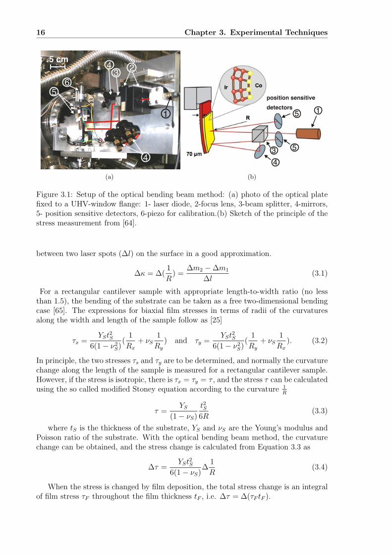
Figure 3.2: The position signals from the detectors during epitaxial growth of Fe mono-layers on Ir(100)-(5×1)Hex. Two detectors are illuminated by the laser beams andreflected from the upper (SGNTOP) and lower (SGNBOT) part of the sample sur-face. The relation between signal voltage and the deflection of the beam —calibrationfactor— is obtained using a piezo translation of the detectors.
The two optical beam bending method takes advantages of [66]: (a) direct curvaturemeasurement with high precision, and (b) enhanced signal-to-noise ratio by eliminatingthe common noise of the two signals with a difference measurement. An example ofa stress measurement during deposition is shown in Figure 3.2. The position signalobtained from two position sensitive detectors are transformed into deflections of thesample at two positions, and the curvature change of the sample is calculated from thedeflections using Equation 3.1. Finally the stress change is obtained according to thecurvature change.
The mismatch between the epitaxial film and the substrate induces a stress in theorder of GPa that corresponds to a curvature change of several (km)−1. But the magne-toelastic coupling induced stress change is two orders of magnitude smaller which makesit more demanding to be measured. The two optical beam bending method is used inthis work to measure the magnetoelastic coupling induced stress change in the magneticmonolayers of Fe, Co and Ni on Ir(100) substrate (as illustrated in Figure 3.3(a)). Thesample is put into magnetic fields (Figure 3.4) that can force the magnetization to be
18 Chapter 3. Experimental Techniques
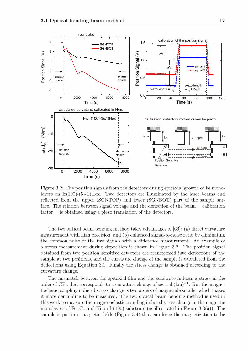
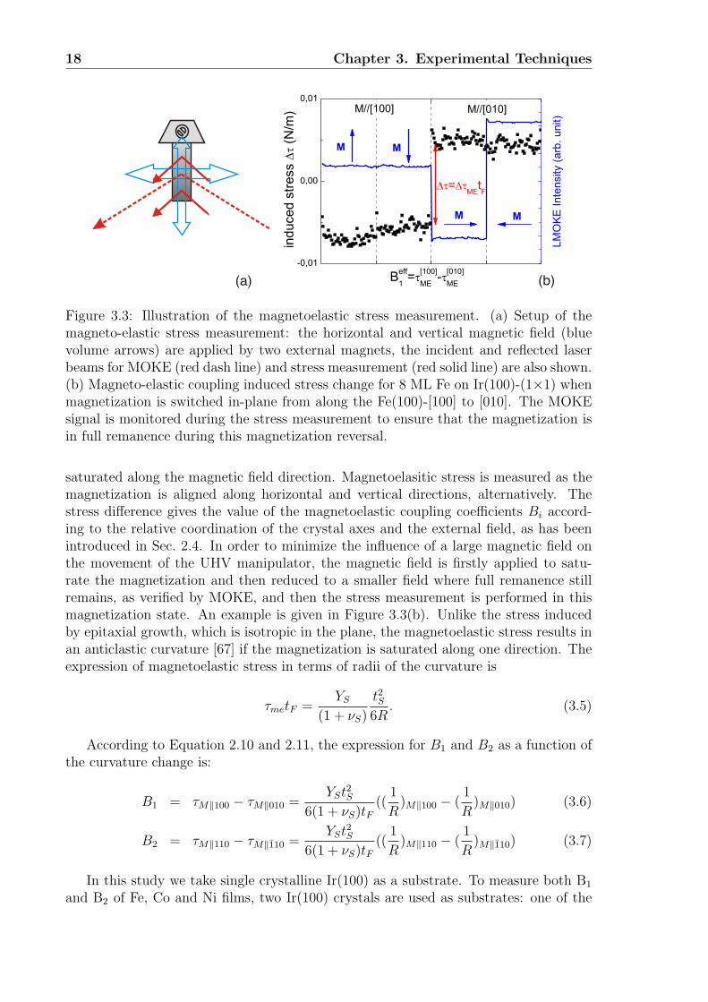
(a) (b)Figure 3.3: Illustration of the magnetoelastic stress measurement. (a) Setup of themagneto-elastic stress measurement: the horizontal and vertical magnetic field (bluevolume arrows) are applied by two external magnets, the incident and reflected laserbeams for MOKE (red dash line) and stress measurement (red solid line) are also shown.(b) Magneto-elastic coupling induced stress change for 8 ML Fe on Ir(100)-(1×1) whenmagnetization is switched in-plane from along the Fe(100)-[100] to [010]. The MOKEsignal is monitored during the stress measurement to ensure that the magnetization isin full remanence during this magnetization reversal.
saturated along the magnetic field direction. Magnetoelasitic stress is measured as themagnetization is aligned along horizontal and vertical directions, alternatively. Thestress difference gives the value of the magnetoelastic coupling coefficients Bi accord-ing to the relative coordination of the crystal axes and the external field, as has beenintroduced in Sec. 2.4. In order to minimize the influence of a large magnetic field onthe movement of the UHV manipulator, the magnetic field is firstly applied to satu-rate the magnetization and then reduced to a smaller field where full remanence stillremains, as verified by MOKE, and then the stress measurement is performed in thismagnetization state. An example is given in Figure 3.3(b). Unlike the stress inducedby epitaxial growth, which is isotropic in the plane, the magnetoelastic stress results inan anticlastic curvature [67] if the magnetization is saturated along one direction. Theexpression of magnetoelastic stress in terms of radii of the curvature is
τmetF =YS
(1 + νS)
t2S6R
. (3.5)
According to Equation 2.10 and 2.11, the expression for B1 and B2 as a function ofthe curvature change is:
B1 = τM‖100 − τM‖010 =YSt2S
6(1 + νS)tF((
1
R)M‖100 − (
1
R)M‖010) (3.6)
B2 = τM‖110 − τM‖110 =YSt2S
6(1 + νS)tF((
1
R)M‖110 − (
1
R)M‖110) (3.7)
In this study we take single crystalline Ir(100) as a substrate. To measure both B1
and B2 of Fe, Co and Ni films, two Ir(100) crystals are used as substrates: one of the
3.2 The ultra high vacuum (UHV) system 19
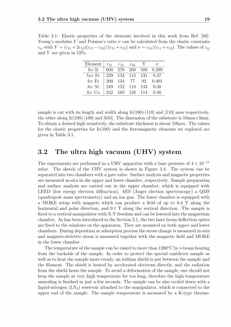
Table 3.1: Elastic properties of the elements involved in this work from Ref. [68].Young’s modulus Y and Poisson’s ratio ν can be calculated from the elastic constantscij with Y = (c11 + 2c12)(c11− c12)/(c11 + c12) and ν = c12/(c11 + c12). The values of cij
and Y are given in GPa.
Element c11 c12 c44 Y νfcc Ir 600 270 260 500 0.299bcc Fe 229 134 115 131 0.37fcc Fe 200 134 77 92 0.401fcc Ni 249 152 118 133 0.38fcc Co 242 160 128 114 0.40
sample is cut with its length and width along Ir(100)-[110] and [110] axes respectively,the other along Ir(100)-[100] and [010]. The dimension of the substrate is 10mm×3mm.To obtain a desired high sensitivity, the substrate thickness is about 100µm. The valuesfor the elastic properties for Ir(100) and the ferromagnetic elements we explored aregiven in Table 3.1.
3.2 The ultra high vacuum (UHV) system
The experiments are performed in a UHV apparatus with a base pressure of 4× 10⁻¹¹
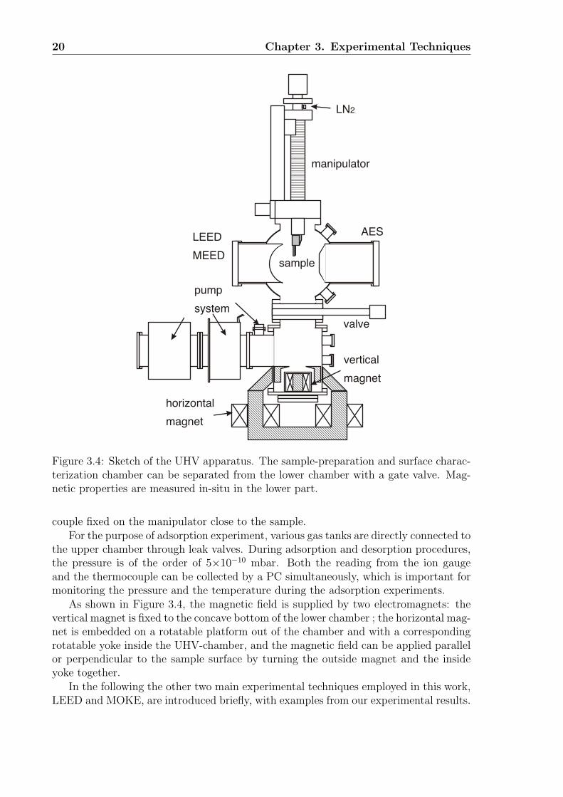
mbar. The sketch of the UHV system is shown in Figure 3.4. The system can beseparated into two chambers with a gate valve. Surface analysis and magnetic propertiesare measured in-situ in the upper and lower chamber, respectively. Sample preparationand surface analysis are carried out in the upper chamber, which is equipped withLEED (low energy electron diffraction), AES (Auger election spectroscopy) a QMS(quadrupole mass spectrometry) and an ion gun. The lower chamber is equipped witha MOKE setup with magnets which can produce a field of up to 0.4 T along thehorizontal and polar direction, and 0.1 T along the vertical direction. The sample isfixed to a vertical manipulator with X-Y freedom and can be lowered into the magnetismchamber. As has been introduced in the Section 3.1, the two laser beam deflection opticsare fixed to the windows on the apparatus. They are mounted on both upper and lowerchambers. During deposition or adsorption process the stress change is measured in-situand magneto-strictive stress is measured together with the magnetic field and MOKEin the lower chamber .
The temperature of the sample can be raised to more than 1200◦C by e-beam heatingfrom the backside of the sample. In order to protect the special cantilever sample aswell as to heat the sample more evenly, an iridium shield is put between the sample andthe filament. The shield is heated by accelerated electrons directly, and the radiationfrom the shield heats the sample. To avoid a deformation of the sample, one should notkeep the sample at very high temperature for too long, therefore the high temperatureannealing is finished in just a few seconds. The sample can be also cooled down with aliquid-nitrogen (LN2) reservoir attached to the manipulator, which is connected to theupper end of the sample. The sample temperature is measured by a K-type thermo-
20 Chapter 3. Experimental Techniques
LEEDMEED AESpumpsystem
horizontal magnetverticalmagnet
manipulator
samplevalve
LN2
Figure 3.4: Sketch of the UHV apparatus. The sample-preparation and surface charac-terization chamber can be separated from the lower chamber with a gate valve. Mag-netic properties are measured in-situ in the lower part.
couple fixed on the manipulator close to the sample.For the purpose of adsorption experiment, various gas tanks are directly connected to
the upper chamber through leak valves. During adsorption and desorption procedures,the pressure is of the order of 5×10⁻¹⁰ mbar. Both the reading from the ion gaugeand the thermocouple can be collected by a PC simultaneously, which is important formonitoring the pressure and the temperature during the adsorption experiments.
As shown in Figure 3.4, the magnetic field is supplied by two electromagnets: thevertical magnet is fixed to the concave bottom of the lower chamber ; the horizontal mag-net is embedded on a rotatable platform out of the chamber and with a correspondingrotatable yoke inside the UHV-chamber, and the magnetic field can be applied parallelor perpendicular to the sample surface by turning the outside magnet and the insideyoke together.
In the following the other two main experimental techniques employed in this work,LEED and MOKE, are introduced briefly, with examples from our experimental results.
3.2 The ultra high vacuum (UHV) system 21
(01)(11)
100 eVIr(100)-(1x1)ScreenWindow
e-gun Samplee-
UHVvideocamera
PC Control Panel
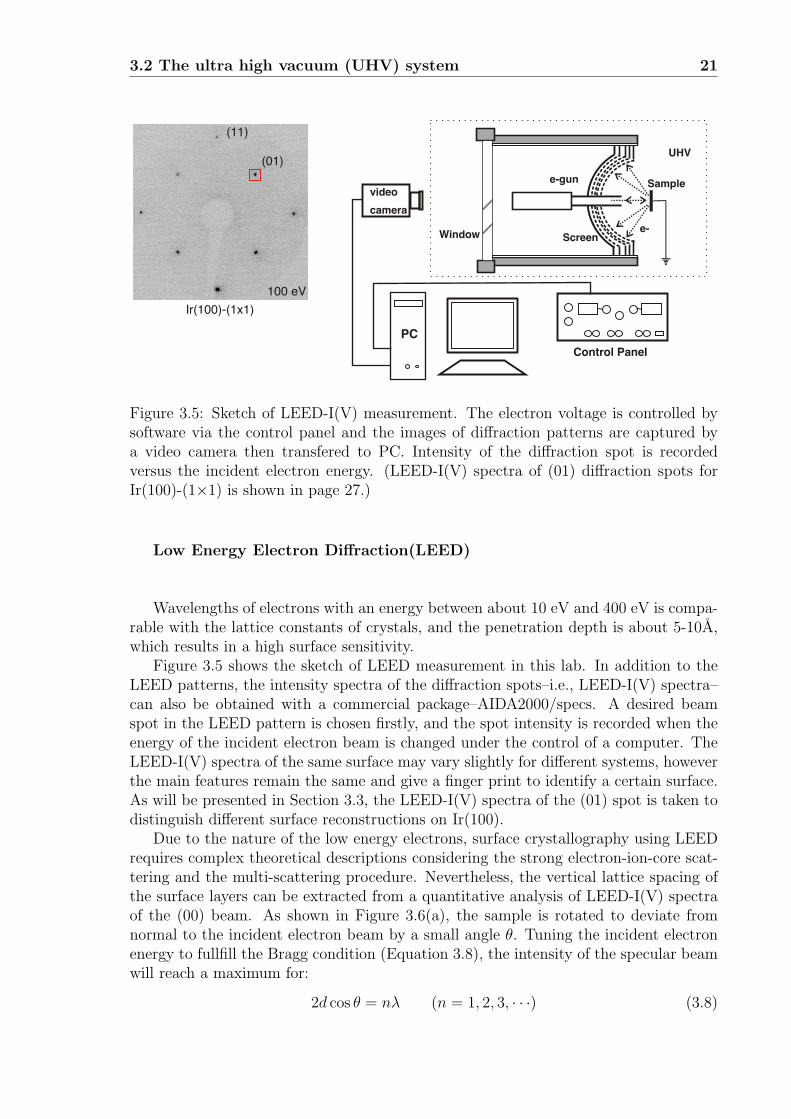
Figure 3.5: Sketch of LEED-I(V) measurement. The electron voltage is controlled bysoftware via the control panel and the images of diffraction patterns are captured bya video camera then transfered to PC. Intensity of the diffraction spot is recordedversus the incident electron energy. (LEED-I(V) spectra of (01) diffraction spots forIr(100)-(1×1) is shown in page 27.)
Low Energy Electron Diffraction(LEED)
Wavelengths of electrons with an energy between about 10 eV and 400 eV is compa-rable with the lattice constants of crystals, and the penetration depth is about 5-10A,which results in a high surface sensitivity.
Figure 3.5 shows the sketch of LEED measurement in this lab. In addition to theLEED patterns, the intensity spectra of the diffraction spots–i.e., LEED-I(V) spectra–can also be obtained with a commercial package–AIDA2000/specs. A desired beamspot in the LEED pattern is chosen firstly, and the spot intensity is recorded when theenergy of the incident electron beam is changed under the control of a computer. TheLEED-I(V) spectra of the same surface may vary slightly for different systems, howeverthe main features remain the same and give a finger print to identify a certain surface.As will be presented in Section 3.3, the LEED-I(V) spectra of the (01) spot is taken todistinguish different surface reconstructions on Ir(100).
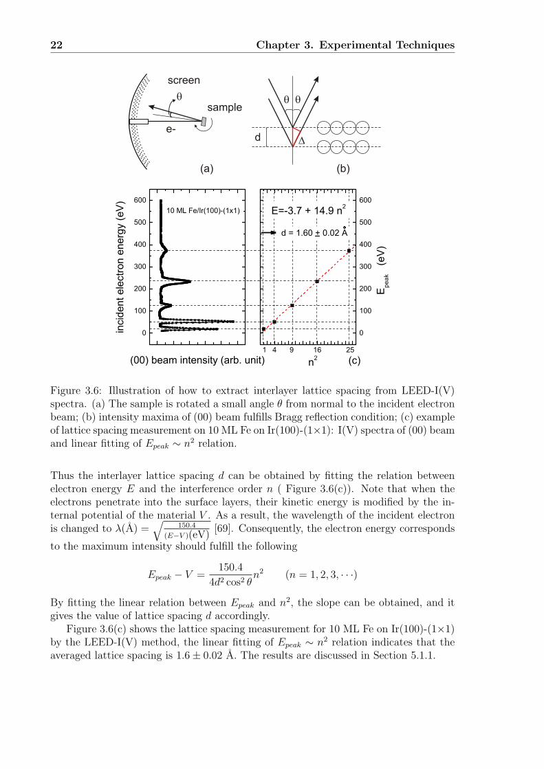
Due to the nature of the low energy electrons, surface crystallography using LEEDrequires complex theoretical descriptions considering the strong electron-ion-core scat-tering and the multi-scattering procedure. Nevertheless, the vertical lattice spacing ofthe surface layers can be extracted from a quantitative analysis of LEED-I(V) spectraof the (00) beam. As shown in Figure 3.6(a), the sample is rotated to deviate fromnormal to the incident electron beam by a small angle θ. Tuning the incident electronenergy to fullfill the Bragg condition (Equation 3.8), the intensity of the specular beamwill reach a maximum for:
2d cos θ = nλ (n = 1, 2, 3, · · ·) (3.8)
22 Chapter 3. Experimental Techniques
!d "
! samplescreene-
!
(a) (b)
Figure 3.6: Illustration of how to extract interlayer lattice spacing from LEED-I(V)spectra. (a) The sample is rotated a small angle θ from normal to the incident electronbeam; (b) intensity maxima of (00) beam fulfills Bragg reflection condition; (c) exampleof lattice spacing measurement on 10 ML Fe on Ir(100)-(1×1): I(V) spectra of (00) beamand linear fitting of Epeak ∼ n2 relation.
Thus the interlayer lattice spacing d can be obtained by fitting the relation betweenelectron energy E and the interference order n ( Figure 3.6(c)). Note that when theelectrons penetrate into the surface layers, their kinetic energy is modified by the in-ternal potential of the material V . As a result, the wavelength of the incident electronis changed to λ(A) =
√150.4
(E−V )(eV)[69]. Consequently, the electron energy corresponds
to the maximum intensity should fulfill the following
Epeak − V =150.4
4d2 cos2 θn2 (n = 1, 2, 3, · · ·)
By fitting the linear relation between Epeak and n2, the slope can be obtained, and itgives the value of lattice spacing d accordingly.
Figure 3.6(c) shows the lattice spacing measurement for 10 ML Fe on Ir(100)-(1×1)by the LEED-I(V) method, the linear fitting of Epeak ∼ n2 relation indicates that theaveraged lattice spacing is 1.6± 0.02 A. The results are discussed in Section 5.1.1.
3.2 The ultra high vacuum (UHV) system 23
transverselongitudinal
polaranalyzerpolarizerp
sps p
sPEM
detectorlaser diode
sample1/4 waveplate
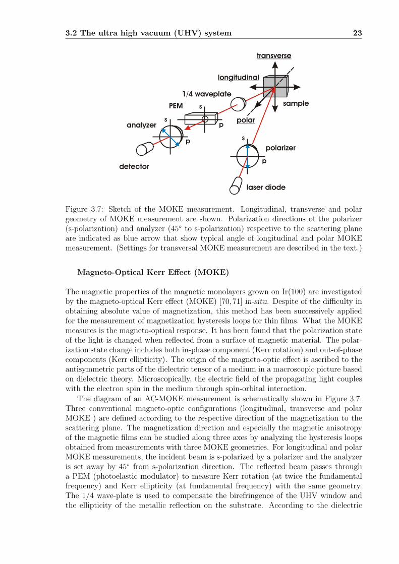
Figure 3.7: Sketch of the MOKE measurement. Longitudinal, transverse and polargeometry of MOKE measurement are shown. Polarization directions of the polarizer(s-polarization) and analyzer (45◦ to s-polarization) respective to the scattering planeare indicated as blue arrow that show typical angle of longitudinal and polar MOKEmeasurement. (Settings for transversal MOKE measurement are described in the text.)
Magneto-Optical Kerr Effect (MOKE)
The magnetic properties of the magnetic monolayers grown on Ir(100) are investigatedby the magneto-optical Kerr effect (MOKE) [70,71] in-situ. Despite of the difficulty inobtaining absolute value of magnetization, this method has been successively appliedfor the measurement of magnetization hysteresis loops for thin films. What the MOKEmeasures is the magneto-optical response. It has been found that the polarization stateof the light is changed when reflected from a surface of magnetic material. The polar-ization state change includes both in-phase component (Kerr rotation) and out-of-phasecomponents (Kerr ellipticity). The origin of the magneto-optic effect is ascribed to theantisymmetric parts of the dielectric tensor of a medium in a macroscopic picture basedon dielectric theory. Microscopically, the electric field of the propagating light coupleswith the electron spin in the medium through spin-orbital interaction.
The diagram of an AC-MOKE measurement is schematically shown in Figure 3.7.Three conventional magneto-optic configurations (longitudinal, transverse and polarMOKE ) are defined according to the respective direction of the magnetization to thescattering plane. The magnetization direction and especially the magnetic anisotropyof the magnetic films can be studied along three axes by analyzing the hysteresis loopsobtained from measurements with three MOKE geometries. For longitudinal and polarMOKE measurements, the incident beam is s-polarized by a polarizer and the analyzeris set away by 45◦ from s-polarization direction. The reflected beam passes througha PEM (photoelastic modulator) to measure Kerr rotation (at twice the fundamentalfrequency) and Kerr ellipticity (at fundamental frequency) with the same geometry.The 1/4 wave-plate is used to compensate the birefringence of the UHV window andthe ellipticity of the metallic reflection on the substrate. According to the dielectric
24 Chapter 3. Experimental Techniques
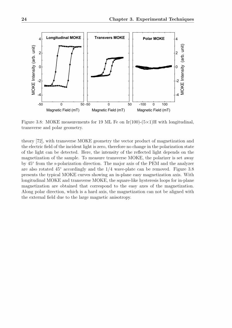
Figure 3.8: MOKE measurements for 19 ML Fe on Ir(100)-(5×1)H with longitudinal,transverse and polar geometry.
theory [72], with transverse MOKE geometry the vector product of magnetization andthe electric field of the incident light is zero, therefore no change in the polarization stateof the light can be detected. Here, the intensity of the reflected light depends on themagnetization of the sample. To measure transverse MOKE, the polarizer is set awayby 45◦ from the s-polarization direction. The major axis of the PEM and the analyzerare also rotated 45◦ accordingly and the 1/4 wave-plate can be removed. Figure 3.8presents the typical MOKE curves showing an in-plane easy magnetization axis. Withlongitudinal MOKE and transverse MOKE, the square-like hysteresis loops for in-planemagnetization are obtained that correspond to the easy axes of the magnetization.Along polar direction, which is a hard axis, the magnetization can not be aligned withthe external field due to the large magnetic anisotropy.
3.3 Preparation of Ir(100) surface reconstructions 25
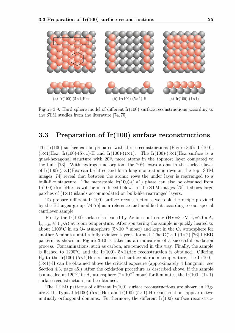
Figure 3.9: Hard sphere model of different Ir(100) surface reconstructions according tothe STM studies from the literature [74,75]
3.3 Preparation of Ir(100) surface reconstructions
The Ir(100) surface can be prepared with three reconstructions (Figure 3.9): Ir(100)-(5×1)Hex, Ir(100)-(5×1)-H and Ir(100)-(1×1). The Ir(100)-(5×1)Hex surface is aquasi-hexagonal structure with 20% more atoms in the topmost layer compared tothe bulk [73]. With hydrogen adsorption, the 20% extra atoms in the surface layerof Ir(100)-(5×1)Hex can be lifted and form long mono-atomic rows on the top. STMimages [74] reveal that between the atomic rows the under layer is rearranged to abulk-like structure. The metastable Ir(100)-(1×1) phase can also be obtained fromIr(100)-(5×1)Hex as will be introduced below. In the STM images [75] it shows largepatches of (1×1) islands accommodated on bulk-like rearranged layers.
To prepare different Ir(100) surface reconstructions, we took the recipe providedby the Erlangen group [74, 75] as a reference and modified it according to our specialcantilever sample.
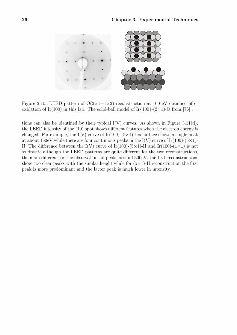
Firstly the Ir(100) surface is cleaned by Ar ion sputtering (HV=3 kV, Ie=20 mA,Isample ≈ 1 µA) at room temperature. After sputtering the sample is quickly heated toabout 1100◦C in an O2 atmosphere (5×10⁻⁶ mbar) and kept in the O2 atmosphere foranother 5 minutes until a fully oxidized layer is formed. The O(2×1+1×2) [76] LEEDpattern as shown in Figure 3.10 is taken as an indication of a successful oxidationprocess. Contaminations, such as carbon, are removed in this way. Finally, the sampleis flashed to 1200◦C and the Ir(100)-(5×1)Hex reconstruction is obtained. OfferingH2 to the Ir(100)-(5×1)Hex reconstructed surface at room temperature, the Ir(100)-(5×1)-H can be obtained above the critical exposure (approximately 4 Langmuir, seeSection 4.3, page 45.) After the oxidation procedure as described above, if the sampleis annealed at 120◦C in H2 atmosphere (2×10⁻⁷ mbar) for 5 minutes, the Ir(100)-(1×1)surface reconstruction can be obtained.
The LEED patterns of different Ir(100) surface reconstructions are shown in Fig-ure 3.11. Typical Ir(100)-(5×1)Hex and Ir(100)-(5×1)-H reconstructions appear in twomutually orthogonal domains. Furthermore, the different Ir(100) surface reconstruc-
26 Chapter 3. Experimental Techniques
Figure 3.10: LEED pattern of O(2×1+1×2) reconstruction at 100 eV obtained afteroxidation of Ir(100) in this lab. The solid-ball model of Ir{100}-(2×1)-O from [76] .
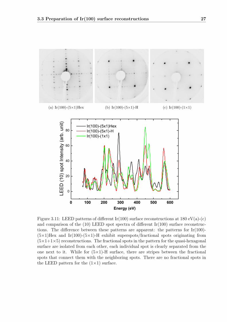
tions can also be identified by their typical I(V) curves. As shown in Figure 3.11(d),the LEED intensity of the (10) spot shows different features when the electron energy ischanged. For example, the I(V) curve of Ir(100)-(5×1)Hex surface shows a single peakat about 150eV while there are four continuous peaks in the I(V) curve of Ir(100)-(5×1)-H. The difference between the I(V) curve of Ir(100)-(5×1)-H and Ir(100)-(1×1) is notso drastic although the LEED patterns are quite different for the two reconstructions,the main difference is the observations of peaks around 300eV, the 1×1 reconstructionsshow two clear peaks with the similar height while for (5×1)-H reconstruction the firstpeak is more predominant and the latter peak is much lower in intensity.
3.3 Preparation of Ir(100) surface reconstructions 27
Figure 3.11: LEED patterns of different Ir(100) surface reconstructions at 180 eV(a)-(c)and comparison of the (10) LEED spot spectra of different Ir(100) surface reconstruc-tions. The difference between these patterns are apparent: the patterns for Ir(100)-(5×1)Hex and Ir(100)-(5×1)-H exhibit superspots/fractional spots originating from(5×1+1×5) reconstructions. The fractional spots in the pattern for the quasi-hexagonalsurface are isolated from each other, each individual spot is clearly separated from theone next to it. While for (5×1)-H surface, there are stripes between the fractionalspots that connect them with the neighboring spots. There are no fractional spots inthe LEED pattern for the (1×1) surface.