Chapter 3 Machine Translation

Chapter 3

Machine Translation

3.1 Problem (again)Remember that we motivated the language modeling problem by thinking about

machine translation as “deciphering” the source language into the target lan-

guage.

% (5 , 4) = % (4) % (5 | 4) (3.1)

4∗ = arg max

4

% (4 | 5 ) (3.2)

= arg max

4

% (4, 5 )% (5 ) (3.3)

= arg max

4

% (4, 5 ) (3.4)

= arg max

4

% (4) % (5 | 4). (3.5)

In this chapter, we start by focusing on % (5 | 4) (the translation model). We will

also consider so-called direct models that estimate % (4 | 5 ), in particular neural

networks.

All the models we’ll look at are trained on parallel text, which is a corpus of

text that expresses the same meaning in two (or more) di�erent languages. Usu-

ally we assume that a parallel text is already sentence-aligned, that is, it consists

of sentence pairs, each of which expresses the same meaning in two languages.

In the original work on statistical machine translation (Brown et al., 1993), the

source language was French (5 ) and the target language was English (4), and we’ll

use those variables even for other language pairs. Our example uses Spanish and

English.

Here is an example parallel text (Knight, 1999):

1. Garcia and associates

Garcıa y asociados

2. his associates are not strong

sus asociados no son fuertes

35

Chapter 3. Machine Translation 36

3.2 Finite Transducers? (No)A �nite-state transducer is like a �nite-state automaton, but has both an input

alphabet Σ and an output alphabet Σ′. �e transitions look like this:

@ A0 : 0′ / ?

where 0 ∈ Σ∪ {n}, 0′ ∈ Σ′ ∪ {n}, and ? is the weight. �e n stands for the empty

string, so a transition 0 : n means “delete input symbol 0,” and n : 0′means “insert

output symbol 0′.”Weighted �nite transducers have been used with huge success in speech pro-

cessing, morphology, and other tasks (Mohri, 1997; Mohri, Pereira, and Riley,

2002), and we’ll have more to say about them later on when we talk about those

tasks. Given their success, it might seem that �nite transducers would be a great

way to de�ne a translation model % (5 | 4). But a major limitation of transducers

is that they only allow limited reordering. For example, there’s no such thing as a

transducer that inputs a string and outputs the reverse string. Despite valiant ef-

forts to make them work for machine translation (Kumar and Byrne, 2003), they

do not seem to be the right tool.

3.3 IBM ModelsInstead, we turn to a series of �ve models invented at IBM in their original work

on statistical machine translation (Brown et al., 1993).

3.3.1 Word alignment�e IBM models are models of % (5 | 4) that make the simplifying assumption

that each Spanish word depends on exactly one English word. For example:

1. Garcia and associates EOS

Garcıa y asociados EOS

2. his associates are not strong EOS

sus asociados no son fuertes EOS

(We’ve made some slight changes compared to the original paper. Originally,

5 did not end with EOS, and there was a di�erent way to decide when to stop

generating 5 . And 4 did have EOS, but it was called NULL.)

More formally: let Σf and Σe be the Spanish and English vocabularies, and

• 5 = 51 · · · 5= range over Spanish sentences (5= = EOS)

• 4 = 41 · · · 4< range over English sentences (4< = EOS)

CSE 40657/60657: Natural Language Processing Version of August 28, 2021


• 0 = (01, . . . , 0=) range over possible many-to-one alignments, where each

1 ≤ 0 9 ≤ < and 0 9 = 8 means that Spanish word 9 is aligned to English

word 8 .

We will use these variable names throughout this chapter. Remember that 4 , 8 ,

and< come alphabetically before 5 , 9 , and =, respectively.

�us, for our two example sentences, we have

1. 5 = Garcıa y asociados EOS = = 4

4 = Garcia and associates EOS < = 4

0 = (1, 2, 3, 4)

2. 5 = sus asociados no son fuertes EOS = = 6

4 = his associates are not strong EOS < = 6

0 = (1, 2, 4, 3, 5, 6).

�ese alignments 0will be included in our “story” of how an English sentence

4 becomes a Spanish sentence 5 . In other words, we are going to de�ne a model

of % (5 , 0 | 4), not % (5 | 4), and training this model will involve summing over

all alignments 0:

maximize ! =∑

(5 ,4) ∈data

log % (5 | 4) (3.6)

=∑

(5 ,4) ∈data

log

∑0

% (5 , 0 | 4). (3.7)

(�is is similar to training of NFAs in the previous chapter, where there could be

more than one accepting path for a given training string.)

3.3.2 Model 1IBM Model 1 goes like this.

1. Generate each alignment 01, . . . , 0= , each with uniform probability1<

.

2. Generate Spanish words 51, . . . , 5= , each with probability C (59 | 40 9 ).

In equations, the model is:

% (5 , 0 | 4) ==∏9=1

(1

<C (59 | 40 9 )

). (3.8)

�e parameters of the model are the word-translation probabilities C (5 | 4).We want to optimize these parameters to maximize the log-likelihood,

! =∑

(5 ,4) ∈data

log

∑0

% (5 , 0 | 4). (3.9)



�e summation over 0 is over an exponential number of alignments, but we can

rearrange it to make it e�ciently computable:∑0

% (5 , 0 | 4) =∑0

=∏9=1

(1

<C (59 | 40 9 )

)(3.10)

=

<∑01=1

· · ·<∑

0==1

1

<C (51 | 401 ) · · ·

1

<C (5= | 40= ) (3.11)

=

<∑01=1

1

<C (51 | 401 ) · · ·

<∑0==1

1

<C (5= | 40= ) (3.12)

=

=∏9=1

<∑8=1

1

<C (59 | 48 ). (3.13)

�e good news is that this objective function is convex, that is, every local

maximum is a global maximum. �e bad news is that there’s no closed-form

solution for this maximum, so we must use some iterative approximation. �e

classic way to do this is expectation-maximization, but we can also use stochastic

gradient ascent. �e trick is ensuring that the C probabilities sum to one. We do

this by de�ning a matrix T with an element for every pair of Spanish and English

words. �e elements are unconstrained real numbers (called logits), and are the

new parameters of the model. �en we can use the so�max function to change

them into probabilities, which we use as the C probabilities.

T ∈ R |Σf |× |Σe |(3.14)

C (59 | 48 ) =[so�max T∗,48

]59

(3.15)

=exp T59 ,48∑

5 ′∈Σf

exp T5 ′,48. (3.16)

For large datasets, the vast majority of (Spanish word, English word) pairs

never cooccur (that is, in the same sentence pair), which means that the vast

majority of entries of T would be −∞. So to make this practical, we’d have to

store T as a sparse matrix.

3.3.3 Model 2 and beyondIn Model 1, we chose each 0 9 with uniform probability 1/<, which makes for a

very weak model. For example, it’s unable to learn that the �rst Spanish word is

more likely to depend on the �rst English word than (say) the seventh English

word. In Model 2, we replace 1/< with a learnable parameter:

% (5 , 0 | 4) ==∏9=1

(0(8 | 9,<, =) C (59 | 40 9 )

).

where for each 8, 9,<, =, the parameter 0(8 | 9,<, =) must be learned. (�is nota-

tion follows the original paper; I hope it’s not too confusing that 0 9 is an integer

but 0(·) is a probability distribution.) �en we can learn that (say) 0(1 | 1, 10, 10)is high, but 0(7 | 1, 10, 10) is low.



�ere are also Models 3, 4, and 5, which can learn dependencies between the

0 9 , like:

• Distortion: Even if the model gives low probability to 01 = 7, it should be

the case that given 01 = 7, the probability that 02 = 8 is high, because it’s

common for a block of words to move together.

• Fertility: It should be most common for one Spanish word to align to one

English word, less common for zero or two Spanish words to align to one

English word, and extremely rare for ten Spanish words align to one En-

glish word.

But for our purposes, it’s good enough to stop here at Model 2.

To train Model 2 by stochastic gradient ascent, we again need to express the 0

probabilities in terms of unconstrained parameters. Let" and# be the maximum

English and Spanish sentence length, respectively. �en:

A ∈ R"×#×"×# (3.17)

0(8 | 9,<, =) = [so�max A∗, 9,<,=]8 (3.18)

=exp A8, 9,<,=∑8′ exp A8′, 9,<,=

. (3.19)

3.4 From Alignment to AttentionSo far, we’ve been working in the noisy-channel framework,

% (5 , 4) = % (4) % (5 | 4). (3.20)

One reason for doing this is to divide up the translation problem into two parts

so each model (language model and translation model) can focus doing its part

well. But neural networks are rather good at doing two jobs at the same time,

and so modern MT systems don’t take a noisy-channel approach. Instead, they

directly model % (4 | 5 ). Let’s start by rewriting Model 1 in the direct direction:

% (4 | 5 ) =<∏8=1

=∑9=1

1

=

[so�max T∗,59

]48. (3.21)

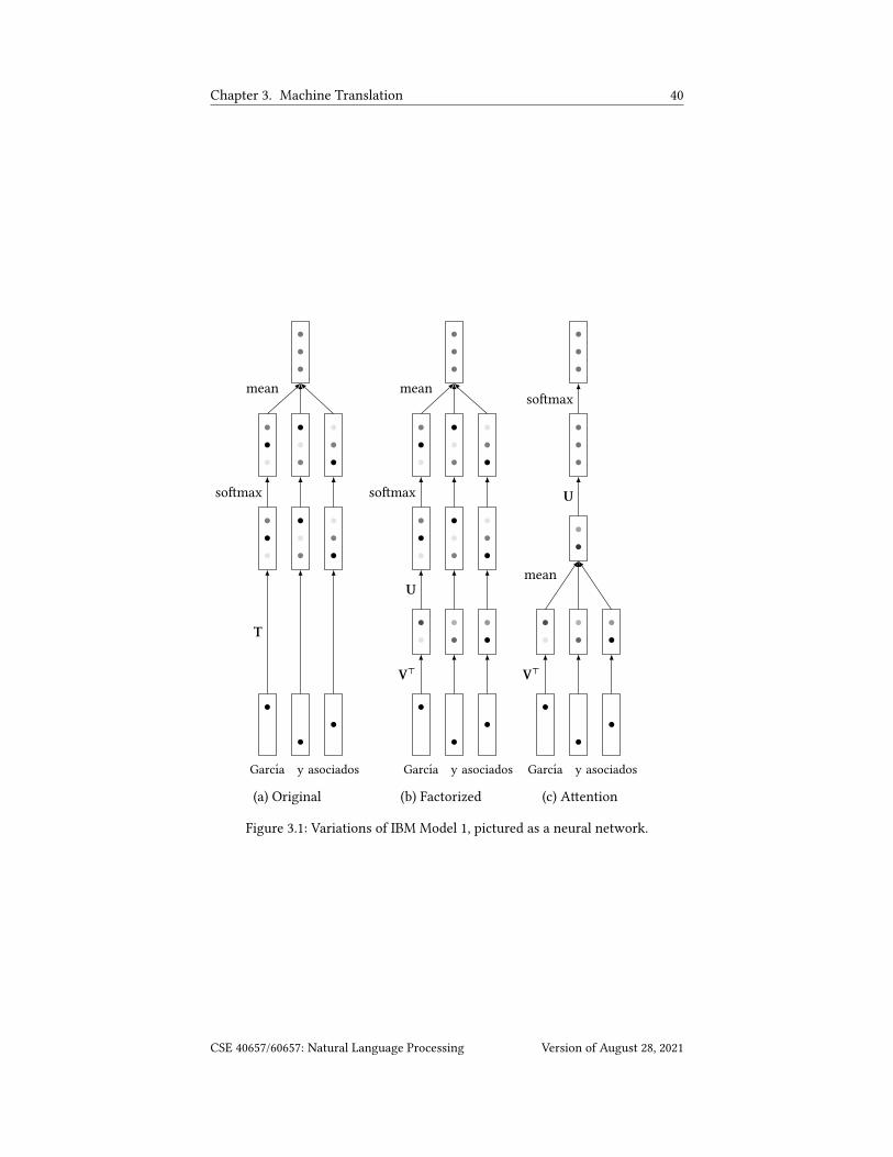
See Figure 3.1a for a picture of this model, drawn in the style of a neural network.

Factoring T. Above, we mentioned that matrix T is very large and sparse. We

can overcome this by factoring it into two smaller matrices (see Figure 3.1b):

U ∈ R |Σe |×3(3.22)

V ∈ R |Σf |×3(3.23)

T = UV> (3.24)

where 3 is some number that we have to choose.



•

Garcıa

•

y

•

asociados

•••

T

•••

•••

•••

so�max

•••

•••

•••

mean

•

Garcıa

•

y

•

asociados

••

V>

••

••

•••

U

•••

•••

•••

so�max

•••

•••

•••

mean

•

Garcıa

•

y

•

asociados

••

V>

••

••

••

mean

•••

U

•••

so�max

(a) Original (b) Factorized (c) A�ention

Figure 3.1: Variations of IBM Model 1, pictured as a neural network.



So the model now looks like

% (4 | 5 ) =<∏8=1

=∑9=1

1

=

[so�max UV59

]48

(3.25)

If you think of T as transforming Spanish words into English words (more

precisely, logits for English words), we’re spli�ing this transformation into two

steps. First, V maps the Spanish word into a size-3 vector, called a word embed-ding. �is transformation V is called an embedding layer because it embeds the

Spanish vocabulary into the vector space R3 which is (somewhat sloppily) called

the embedding space.

Second, U transforms the hidden vector into a vector of logits, one for each

English word. �is transformation U, together with the so�max, are known as a

so�max layer. �e rows of U can also be thought of as embeddings of the English

words.

In fact, for this model, we can think of U and V as embedding both the Spanish

and English vocabularies into the same space. Figure 3.2 shows that if we run

factored Model 1 on a tiny Spanish-English corpus (Knight, 1999) and normalize

the Spanish and English word embeddings, words that are translations of each

other do lie close to each other.

�e choice of 3 ma�ers. If 3 is large enough (at least as big as the smaller

of the two vocabularies), then UV> can compute any transformation that T can.

But if 3 is smaller, then UV> can only be an approximation of the full T (called a

low-rank approximation). �is is a good thing: not only does it solve the sparse-

matrix problem, but it can also generalize be�er. Imagine that we have training

examples

1. El perro es grande.

�e dog is big.

2. El perro es gigante.

�e dog is big.

3. El perro es gigante.

�e dog is large.

�e original Model 1 would not be able to learn a nonzero probability for C (gigante |large). But the factorized model would map both grande and gigante to nearby

embeddings (because both translate to big), and map that region of the space to

large (because gigante translates to large). �us it would learn a nonzero proba-

bility for C (gigante | large).

Attention. To motivate the next change, consider the Spanish-English sentence

pairs

1. por que EOS

why EOS

2. por que EOS

why EOS



40 20 0 20 40

60

40

20

0

20

40

60

.

.

<EOS>

<EOS>

theare

los

associatesasociados

groups

grupos

son

estan

not

sus

no

has

tiene

Garcia

García

clients

and

clientes

y

also

angry

tambien

enfadados

strongfuertes

its

company

three

empresa

tres

Carlos

Carlos

sellvenden

modern

modernos

enemies

enemigos

his

inEurope

en

Europa

la

dozenzanine

zanzanina

pharmaceuticalsmedicinas

smallpequenos

a

una

Figure 3.2: Two-dimensional visualization of the 64-dimensional word embed-

dings learned by the factored Model 1. �e embeddings were normalized and

then projected down to two dimensions using t-SNE (Maaten and Hinton, 2008).

In most cases, the Spanish word embedding is close to its corresponding English

word embedding.



3. por que EOS

why EOS

4. por EOS

for EOS

5. que EOS

what EOS

Here are the probabilities that Model 1 learns:

por que EOS

why 0.49 0.49 0

for 0.33 0 0

what 0 0.33 0

EOS 0.18 0.18 1

It learns a high probabiity for both C (why | por) and C (why | que). In fact, these

probabilities are high enough that if we ask the model to re-translate que EOS, it

will prefer the translation why over what. What went wrong?

When Model 1 looks at the �rst sentence, it imagines that there are two vari-

ants of this sentence, one in which why is translated from por and one in which

why is translated from que. It has no notion of why being translated from both porand que. Nor does it have any way to learn that the absence of por or the absence

of que should “veto” the translation why. Remember that something similar hap-

pened when we took the union of two NFAs, and the solution here is also kind

of similar.

We can �x this if we move the average (

∑=9=1

1=(·)) inside the so�max:

% (4 | 5 ) =<∏8=1

[so�max

(=∑9=1

1

=UV59

)]48

. (3.26)

How does this help? Here’s a near-optimal solution for the logits (the part

inside the so�max):

por que EOS

why 20 20 0

for 30 0 0

what 0 30 0

EOS 10 10 20

Because we’re now averaging logits, not probabilities, there’s a lot more room

for words to in�uence one another’s translations. If we average the columns for

each Spanish sentence, we get:

por que EOS por EOS que EOS

why 40 20 0

for 30 30 0

what 0 0 30

EOS 40 30 30



If por is by itself, then for is the best translation by a lot (10). Similarly if que is by

itself. But if por and que occur together, the score for why goes up to 40, which

is the best translation by a lot (10).

Why is a margin of 10 “a lot”? Because the so�max has an exp in it, so a

margin of 10 becomes a factor of exp 10 ≈ 22000. A�er taking the so�max, we

get something very close to

por que EOS por EOS que EOS

why 0.5 0.0 0.0

for 0.0 0.5 0.0

what 0.0 0.0 0.5

EOS 0.5 0.5 0.5

Since everything inside the so�max is linear, we can move the average to

wherever we want. Let’s move it to in between U and V:

% (4 | 5 ) =<∏8=1

[so�max

(U

=∑9=1

1

=V59

)]48

. (3.27)

�is model is shown in Figure 3.1c. If the V59 can be thought of as vector rep-

resentations of words, then the average

∑91=

V59 can be thought of as a vector

representation of the whole sentence 5 . So the model has two parts, an encoder

(V, then average) which converts 5 to a vector representation of 5 , and a decoder

(U, then so�max) which converts the vector representation to English words.

Now let’s do the same thing to Model 2. Recall that the di�erence between

Model 1 and Model 2 is that we changed the uniform average into a weighted

average, weighted by the parameters 0( 9 | 8). Similarly, here, we can make the

uniform average into a weighted average

% (4 | 5 ) =<∏8=1

[so�max

(U

=∑9=1

0( 9 | 8) V59

)]48

. (3.28)

At each time step 8 , the weights 0( 9 | 8), which must sum to one (

∑9 0( 9 | 8) = 1),

provide a di�erent “view” of 5 . �is mechanism is known as a�ention, and the

network is said to a�end to di�erent parts of the sentence at di�erent times.

�e weights 0( 9 | 8) are called a�ention weights. �ese days, they are usually

computed using dot-product a�ention, which factors 0(· | ·) like we did for C (· | ·)earlier:

Q ∈ R<×3 (3.29)

K ∈ R=×3 (3.30)

0( 9 | 8) = [so�max KQ8 ] 9 (3.31)

For each Spanish word 59 , the network computes a vector K9 , called a key. �is

vector could depend on the position 9 , the word 59 , or any other words in 5 .

�en, at time step 8 , the network computes a vector Q8 , called a query. �is

vector could depend on the position 8 , or the words 41, . . . , 48−1. �e above de�-

nition makes the network a�end most strongly to Spanish words 59 whose keys

K9 are most similar to the query Q8 .



�e vectors that are averaged together (here, the V59 ) are called the values.�ey are frequently (but not always) the same as the keys. And the resulting

weighted average is sometimes called the context vector.To get something similar to Model 2, we would let Q and K be learnable

parameters. More precisely, let " and # be the maximum length of any English

or Spanish or English sentence, respectively, and de�ne learnable parameters

Q ∈ R"×3 (3.32)

K ∈ R#×3 . (3.33)

�e rows of Q and K are called position embeddings (Gehring et al., 2017). �en

for a given Spanish-English sentence pair with lengths = and<, let the queries

and keys be the �rst< and = rows of Q and K, respectively:

Q =

Q1,∗...

Q<,∗

(3.34)

K =

K1,∗...

K=,∗

. (3.35)

3.5 Neural Machine TranslationOur modi�ed Model 2 (eqs. 3.28–3.35) is still not a credible machine translation

system. Its ability to model context on both the source side and target side is very

weak. But there have been two very successful extensions of this model, which

we describe in this section.

3.5.1 Remaining problems�e most glaring problem with our modi�ed Model 2 is that it outputs probabil-

ity distributions for each English word, % (48 | 5 ), but the English words are all

independent of one another. �e string el rıo Jordan can be translated as the riverJordan or the Jordan river, so if

% (42 = river | el rıo Jordan) = 0.5 % (43 = Jordan | el rıo Jordan) = 0.5 (3.36)

% (42 = river | el rıo Jordan) = 0.5 % (43 = Jordan | el rıo Jordan) = 0.5 (3.37)

then the translations the river river and the Jordan Jordan will be just as prob-

able as the river Jordan and the Jordan river. To �x this problem, we need to

make the generation of 48 depend on the previous English words. In the original

noisy-channel approach (% (5 | 4) % (4)), modeling dependencies between En-

glish words was the job of the language model (% (4)), but we threw the language

model out when we switched to a direct approach (% (4 | 5 )).Likewise, on the source side, although we’ve argued that our modi�ed Model

2 can, to a certain extent, translate multiple words like por que at once, it’s not

very sensitive to word order. Indeed, if the model a�ends equally to both words,



it cannot distinguish at all between por que and que por. So we’d like to make the

encoding of a Spanish word also take into account its surrounding context.

3.5.2 PreliminariesPlease note that my descriptions of these models are highly simpli�ed. �ey’re

good enough to get the main idea and to do the homework assignment on ma-

chine translation, but if you should ever need to implement a full-strength trans-

lation model, please consult the original papers or the many online tutorials

about them.

Even simpli�ed, these networks get rather large. To make their de�nitions

more manageable, we break them up into functions. �ese functions usually have

learnable parameters, and to make it unambiguous which function calls share

parameters with which, we introduce the following notation. If a function’s name

has a superscript that looks like 5ℓ

, then its de�nition may contain a parameter

with the same superscript, like Gℓ

. �e ℓ stands for 1, 2, etc., so if we call 51

twice, the same parameter G1

is shared across both calls. But if we call 51

and

52

, they have two di�erent parameters G1

and G2

. (In PyTorch, such functions

would be implemented as modules.)

So, we can de�ne some functions:

Embeddingℓ (:) = E ℓ

:(3.38)

A�ention(q,K,V) =∑9

[so�max Kq] 9 V9 (3.39)

So�maxLayerℓ (x) = so�max(W ℓ x) (3.40)

And now our modi�ed Model 2 (eqs. 3.28–3.35) can be wri�en as:

For 9 = 1, . . . , =:

V9 = Embedding1 (59 ) (3.41)

K9 = Embedding2 ( 9) (3.42)

For 8 = 1, . . . ,<:

q(8) = Embedding3 (8) (3.43)

c(8) = A�ention(q(8) ,K,V) (3.44)

% (48 ) = So�maxLayer4 (c(8) ). (3.45)

3.5.3 Using RNNs�e �rst way to introduce more context sensitivity (Bahdanau, Cho, and Bengio,

2015) is to insert an RNN on both the source and target side (see Figure 3.3). �ese

RNNs are called the encoder and decoder, respectively.

In addition to the functions de�ned above, we need a couple of new ones.

First, a tanh layer:

TanhLayerℓ (x) = tanh(W ℓ x + b ℓ ). (3.46)



•

Garcıa

one-hot vectors

•

y

•

asociados

••RNN encoder

••

••

••context vector

a�ention

•

Garcia

one-hot vectors

•

and

••RNN decoder

••

•••

logits

•••

% (43)

so�max

Figure 3.3: Simpli�ed diagram of an RNN translation model (Bahdanau, Cho, and

Bengio, 2015; Luong, Pham, and Manning, 2015).



To compute one step of an RNN:

RNNCellℓ (h, x) = tanh(A ℓ h + B ℓ x + c ℓ ). (3.47)

Now, the model is de�ned as follows. For 9 = 1, . . . , =, we compute a sequence

of source word embeddings v( 9) ∈ R3 , and use an RNN to compute a sequence

of vectors h( 9) ∈ R3 :

v( 9) = Embedding1 (59 ) 9 = 1, . . . , = (3.48)

h( 9) = RNNCellℓ (h( 9−1) , x( 9) ) 9 = 1, . . . , = (3.49)

where h(0) is a parameter to be learned. It will be convenient to pack the rest of

the h( 9) into a single matrix,

H ∈ R=×3

H = [h(1) · · · h(=) ]>. (3.50)

Usually fancier RNNs (using GRUs or LSTMs) are used instead of a simple RNN

as shown here. Also, it’s quite common to stack up several RNNs, with the output

of one feeding into the input of the next.

�e decoder RNN varies more from model to model; the one shown here is

most similar to that of Luong, Pham, and Manning (2015). Like the encoder, it

has an initial vector g(0) ∈ R3 , which is a parameter to be learned, and computes

a sequence of vectors g(8) :

u(8) = Embedding3 (48 ) 8 = 1, . . . ,< (3.51)

g(8) = RNNCell4 (g(8−1) , u(8) ) 8 = 1, . . . ,<. (3.52)

Rather than immediately trying to predict an output word, we �rst use a�ention

to compute a context vector:

c(8) ∈ R3

c(8) = A�ention(g(8−1) ,H,H) (3.53)

Using the Spanish encodings (H) as the keys and values is very standard, whereas

the choice of queries varies. For simplicity, we’re using the most recent English

word’s encoding (g(8−1) ).So we have an English encoding g(8−1) that summarizes the English sentence

so far (41 · · · 48−1), and a context vector c(8) that summarizes the Spanish sentence.

We concatenate the two and apply a tanh layer to get a single vector:

o(8) ∈ R3

o(8) = TanhLayer5

( [c(8)

g(8−1)

] )(3.54)

And �nally we predict an English word:

% (48 ) = So�maxLayer6 (o(8) ). (3.55)

Important implementation note: Whereas the encoder could be wri�en using

many loops over 9 , the decoder has to be wri�en as a single loop over 8 = 1, . . . , =.

�e order of computation is: c(1) , o(1) , % (41), u(1) , g(1) , c(2) , etc.



3.5.4 Using self-attention: Transformers�e other successful neural translation model, which is the current state of the

art, is called the Transformer (Vaswani et al., 2017). �e key idea here is to rec-

ognize that a�ention is not just useful for linking the source and target sides of

the model; it can transform a sequence into a sequence of the same length, and

therefore be used as a replacement for RNNs (Figure 3.4).

We de�ne a new self-a�ention layer, which applies three di�erent linear trans-

formations to the same sequence of vectors to get queries, keys, and values. �en

it uses a�ention to compute a sequence of context vectors.

SelfA�entionCellℓ (X, 8) = A�ention(W ℓ

QX8 ,K,V) (3.56)

where K9 = W ℓ

KX9 (3.57)

V9 = W ℓ

VX9 (3.58)

SelfA�entionℓ (X) = C (3.59)

where C8 = SelfA�entionCellℓ (X, 8). (3.60)

Like an RNN, it maps a sequence of = vectors to a sequence of = vectors, and so

it can, in principle, be used as a drop-in replacement for an RNN.

�ey’re not the same, though – self-a�ention is be�er at learning long-distance

dependencies, but (like Model 1) it knows nothing about word order. �e solution

is surprisingly simple: augment word embeddings with position embeddings.

�en the vector representation of a word token will depend both on the word

type and its position, and the model has the potential to be sensitive to word

order.

�e model is de�ned as follows. We represent the source words as word em-

beddings plus position embeddings:

V ∈ R=×3

V9 = Embedding1 (59 ) + Embedding

2 ( 9) 9 = 1, . . . , = (3.61)

Next comes a self-a�ention layer:

H ∈ R=×3

H = SelfA�ention3 (V). (3.62)

�e self-a�ention layer is always followed by a position-wise feedforward net-work:

H′ ∈ R=×3

H′9 = TanhLayer4 (H9 ) 9 = 1, . . . , =. (3.63)

�en, steps (3.62–3.63) are repeated: SelfA�ention5

, TanhLayer6

, and so

on, usually with 4 or 6 repetitions in total. To avoid running out of le�ers of the

alphabet, though, we don’t write equations for any more repetitions.

�e decoder is also a stack of self-a�ention layers, and again we need to write

the equations using a single iteration over 8 . For each time step 8 = 1, . . . , = − 1,



•

Garcıa

•

y

•

asociados

••

••

••

••

••

••

self-a�ention

••

••

••

••

••

••

self-a�ention

••

••

••

••

cross-a�ention

•

Garcia

•

and

••

••

••

••

self-a�ention

••

••

••

••

self-a�ention

•••

% (43)

Figure 3.4: Simpli�ed diagram of a Transformer translation model (Vaswani et

al., 2017).



we want to predict the next English word, % (48+1). Start by computing the vector

representation of 48 :

u(8) ∈ R3

u(8) = Embedding7 (48 ) + Embedding

8 (8). (3.64)

�en self-a�ention and feedforward layers, but note that at each time step 8 , self-

a�ention only operates on u(1) , . . . , u(8) because it can’t see the future:

g(8) ∈ R3

g(8) = SelfA�entionCell9 ( [u(1) · · · u(8) ]>, 8) (3.65)

g′ (8) ∈ R3

g′ (8) = TanhLayer10 (g(8) ). (3.66)

Now, just as in the RNN-based model, we have a sequence of source encod-

ings and a sequence of target encodings, and the rest of (our simpli�ed version

of) the model proceeds as before (cf. eqs. 3.53–3.55).

c(8) ∈ R3

c(8) = A�ention(g′ (8−1) ,H′,H′) (3.67)

o(8) ∈ R3

o(8) = TanhLayer5

( [c(8)

g′ (8−1)

] )(3.68)

% (48 ) = So�maxLayer6 (o(8) ). (3.69)

Vector g′(0) is a parameter to be learned.1

�e real Transformer is more complicated – in particular, there are actually

multiple cross-a�entions, one a�er each decoder self-a�ention – but hopefully

this su�ces to get the main idea across.

ReferencesBahdanau, Dzmitry, Kyunghyun Cho, and Yoshua Bengio (2015). “Neural Ma-

chine Translation by Jointly Learning to Align and Translate”. In: Proc. ICLR.

url: https://arxiv.org/abs/1409.0473.

Brown, Peter F. et al. (1993). “�e Mathematics of Statistical Machine Translation:

Parameter Estimation”. In: Computational Linguistics 19, pp. 263–311.

Gehring, Jonas et al. (2017). “Convolutional Sequence to Sequence Learning”. In:

Proc. ICML.

Knight, Kevin (1999). A Statistical MT Tutorial Workbook. Notes for the JHU CLSP

Summer Workshop. url: https://kevincrawfordknight.github.io/

papers/wkbk.pdf.

1�e standard formulation doesn’t need this because it prepends BOS to every sentence. I decided

not to prepend BOS in order to get a more uni�ed treatment of automata, RNNs, the IBM models, and

NMT, and painted myself into this corner.


https://arxiv.org/abs/1409.0473

https://kevincrawfordknight.github.io/papers/wkbk.pdf

https://kevincrawfordknight.github.io/papers/wkbk.pdf


Kumar, Shankar and William Byrne (2003). “A Weighted Finite State Transducer

Implementation of the Alignment Template Model for Statistical Machine

Translation”. In: Proceedings of the 2003 Human Language Technology Con-ference of the North American Chapter of the Association for ComputationalLinguistics, pp. 142–149. url: https://aclanthology.org/N03-1019.

Luong, �ang, Hieu Pham, and Christopher D. Manning (Sept. 2015). “E�ective

Approaches to A�ention-based Neural Machine Translation”. In: Proceedingsof the 2015 Conference on Empirical Methods in Natural Language Process-ing. Lisbon, Portugal: Association for Computational Linguistics, pp. 1412–

1421. doi: 10.18653/v1/D15- 1166. url: https://www.aclweb.org/

anthology/D15-1166.

Maaten, Laurens van der and Geo�rey Hinton (2008). “Visualizing High-Dimensional

Data Using t-SNE”. In: Journal of Machine Learning Research 9, pp. 2579–2605.

Mohri, Mehryar (1997). Finite-State Transducers and Language and Speech Pro-cessing.

Mohri, Mehryar, Fernando Pereira, and Michael Riley (2002). “Weighted �nite-

state transducers in speech recognition”. In: Computer Speech and Language16, pp. 69–88.

Vaswani, Ashish et al. (2017). “A�ention is All You Need”. In: Proc. NeurIPS,

pp. 5998–6008. url: https://papers.nips.cc/paper/7181-attention-

is-all-you-need.


https://aclanthology.org/N03-1019

https://doi.org/10.18653/v1/D15-1166

https://www.aclweb.org/anthology/D15-1166

https://www.aclweb.org/anthology/D15-1166

https://papers.nips.cc/paper/7181-attention-is-all-you-need

https://papers.nips.cc/paper/7181-attention-is-all-you-need

Date post:	12-Feb-2022
Category:	Documents
Upload:	others
View:	8 times
Download:	0 times

Chapter 3 Machine Translation

Documents