1 Chapter 3 Taxes, Tax Reform, Public Goods, and Steady-State Models Introduces Auxiliary Variables, Constraints, and Rationing In this chapter, we will begin with a simple problem in which there are taxes in the initial benchmark data, to illustrate how to calibrate a model with existing taxes. Then we will consider labor taxes with endogenous labor supply. These models will make the point that some taxes are less distortionary than others. However, replacing one tax with another rarely yields the same revenue in general equilibrium. Thus our third example will show how to model tax reforms that yield the government the same amount of revenue, referred to as “equal-yield tax reform”. In doing so, we will introduce a major feature of MPS/GE, the auxiliary variable and the constraint equation. The new tax rate will be an endogenous tax, whose value is set in general equilibrium by the revenue constraint. Next, we will introduce a public good, and show how that is modeled. Then we will set the tax rate to finance this public good endogenously according to the Samuelson rule for pure public goods. This will also involve the use of an endogenous tax rate, an auxiliary variable, and a constraint equation. But it will also involve the introduction of another new feature, the rationing constraint.
Transcript
1
Chapter 3Taxes, Tax Reform, Public Goods, and Steady-State ModelsIntroduces Auxiliary Variables, Constraints, and Rationing
In this chapter, we will begin with a simple problem in which there are taxes in theinitial benchmark data, to illustrate how to calibrate a model with existing taxes. Thenwe will consider labor taxes with endogenous labor supply.
These models will make the point that some taxes are less distortionary than others. However, replacing one tax with another rarely yields the same revenue in generalequilibrium. Thus our third example will show how to model tax reforms that yield thegovernment the same amount of revenue, referred to as “equal-yield tax reform”. Indoing so, we will introduce a major feature of MPS/GE, the auxiliary variable and theconstraint equation. The new tax rate will be an endogenous tax, whose value is set ingeneral equilibrium by the revenue constraint.
Next, we will introduce a public good, and show how that is modeled. Then we willset the tax rate to finance this public good endogenously according to the Samuelson rulefor pure public goods. This will also involve the use of an endogenous tax rate, anauxiliary variable, and a constraint equation. But it will also involve the introduction ofanother new feature, the rationing constraint.
2
Finally, we will end this chapter with two other extensions that are valuable forpolicy analysis. First, we will consider taxes and classical unemployment. Second, wewill consider an endogenous capital stock that adjusts according to a steady-state rule. Comparative statics experiments are then comparative steady-state experiments, showingthe general-equilibrium change in all variables after the capital stock has adjusted.
M31.GMS introduces taxes in the benchmark
M32.GMS labor supply and labor tax
M33.GMS introduces equal yield tax reform
M34.GMS introduces a public good
M35.GMS public good provision using a Samuelson rule
M36.GMS taxes and classical unemployment
M37.GMS steady-state capital stock
3
Model M31 taxes in the benchmark data
A positive tax and tax revenue are present in the benchmark data. The first task of isagain to construct a micro-consistent data set. Remember that entries are values.
Under this convention, each tax should be added as a row to the matrix. Taxes arenegative entries in a column indicating payments by a sector. There is a correspondingpositive entry somewhere. In the present case, the tax is simply redistributed lump sumto the consumer, so the consumer gets a positive entry of the tax revenue. A zero rowsum for the tax indicates that all tax receipts must be paid to someone.
The data indicate that the X sector receives 100 units of revenue, of which 20 is paidin taxes. This 20 is received as part of the consumer’s income. Note that these data donot indicate what type of tax is in place. It could be a tax on X output, on all the inputs,or on just one input. We interpret this as a tax on the labor input into sector X.
A crucial task for the modeler is to keep track of what prices firms and consumersface. It is (generally) not possible to calibrate a benchmark equilibrium with all pricesequal to one. For example, if a production input is taxed, then if its consumer price (pricereceived by the consumer) is chosen to be equal to one, then producer price (price paidby the producer) is specified as (1 + t). On the other hand, if the producer price is unity,the consumer price is 1/(1+t). We will discuss output taxes shortly.
Given that we interpret the above data as a tax on the labor input into the X sector,the data tell us that the tax rate is 100%. The amount paid by the X sector to labor (20) isequal to the tax revenue (20). Thus if we set the consumer price of labor to 1 (also theprice to the Y sector), then the price of labor to the X sector must be 2.
When the benchmark price of a production input or output is not equal to unity, it isnecessary to add a reference price field to the production block. The relative prices of
5
inputs fix the marginal rate of substitution (on inputs, marginal rate of transformation onoutputs). Benchmark reference prices and reference quantities are needed in order tocorrectly fit (calibrate) the technology to the data. If these fields are not correctlyspecified, then a run of the model will not reproduce the benchmark data as anequilibrium.
Here is the correct specification of the X production block (recall that default pricesequal 1 so only prices not equal to 1 must be specified).
where TLX (for tax on labor in X) is declared as a parameter elsewhere in the file, inorder to permit changes in TLX as counterfactual experiments.
There are two common mistakes that you need to avoid. First is to leave out theprice field thinking that the assignment of the tax will do that for you. That is incorrect,the P:2 must appear in the block. The tax itself is not used in the calibration, the Q and Pfields are.
6
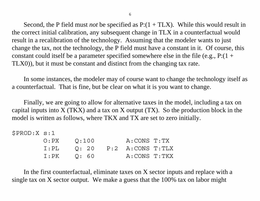
Second, the P field must not be specified as P:(1 + TLX). While this would result inthe correct initial calibration, any subsequent change in TLX in a counterfactual wouldresult in a recalibration of the technology. Assuming that the modeler wants to justchange the tax, not the technology, the P field must have a constant in it. Of course, thisconstant could itself be a parameter specified somewhere else in the file (e.g., P:(1 +TLX0)), but it must be constant and distinct from the changing tax rate.
In some instances, the modeler may of course want to change the technology itself asa counterfactual. That is fine, but be clear on what it is you want to change.
Finally, we are going to allow for alternative taxes in the model, including a tax oncapital inputs into X (TKX) and a tax on X output (TX). So the production block in themodel is written as follows, where TKX and TX are set to zero initially.
In the first counterfactual, eliminate taxes on X sector inputs and replace with asingle tax on X sector output. We make a guess that the 100% tax on labor might
7
generate revenue roughly equivalent to a tax of 25% on both inputs: 20 units of revenueis 100% of the benchmark labor input, or 25% of total benchmark inputs of labor andcapital (20 + 60 = 80). Of course, they will not in fact generate the same revenue as othervariables adjust in general equilibrium. Further discussion of this issue is postponed untilmodel M33.
Now consider a tax on X sector output. It is important to understand that the outputtax rate will be different from the corresponding tax rate on all inputs, because the taxbase is different in the two cases. Let mc denote the marginal cost of production (orproducer price) and p denote the price charged to the consumer. This is how MPS/GEinterprets input (ti) versus output (to) taxes.
Tax on all inputs: p = (1 + ti)mcTax on the output: p(1 - to) = mc
Note mc is the tax base for the input tax, and p is the tax base for the output tax. Theseare not the same. The output tax that is equivalent to the tax on all inputs is found by:
(1 + ti) = 1/(1+to)
8
If ti = TLX = TKX = 0.25 as we have assumed in our first counterfactual, then theequivalent output tax is given by to = TX = 0.20. Thus in our second counterfactual, weset the input taxes to zero and the output tax to 0.20.
One more equivalence can be demonstrated with this small model. The final counterfactual demonstrates that a 20% tax on the output of X is the same as a 25%subsidy to the production of Y. Let t be the tax on X and s the subsidy to Y. Formally,we have
Absolute prices may differ depending on the choice of the numeraire, but all quantitiesand welfare are the same.
Here is the program.
9
$TITLE Model M31.GMS: Closed 2x2 Economy - Calibrate to anExisting Tax
TY Proportional output tax on sector Y, TLX Ad-valorem tax on labor inputs to X, TKX Ad-valorem tax on capital inputs to X;
$ONTEXT
$MODEL:M31
$SECTORS: X ! Activity level for sector X Y ! Activity level for sector Y W ! Activity level for sector W (welfare index)
$COMMODITIES: PX ! Price index for commodity X PY ! Price index for commodity Y PL ! Price index for primary factor L (net of tax) PK ! Price index for primary factor K PW ! Price index for welfare
* In the first counterfactual, we replace the tax on * labor inputs* by a uniform tax on both factors:
13
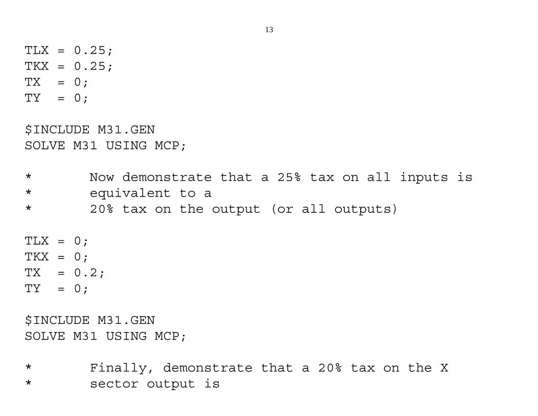
TLX = 0.25; TKX = 0.25;TX = 0;TY = 0;
$INCLUDE M31.GENSOLVE M31 USING MCP;
* Now demonstrate that a 25% tax on all inputs is * equivalent to a* 20% tax on the output (or all outputs)
TLX = 0;TKX = 0;TX = 0.2;TY = 0;
$INCLUDE M31.GENSOLVE M31 USING MCP;
* Finally, demonstrate that a 20% tax on the X* sector output is
14
* equivalent to a 25% subsidy on Y sector output* (assumes that the* funds for the subsidy can be raised lump sum from* the consumer!)
TKX = 0;TLX = 0;TX = 0;TY = -0.25;
$INCLUDE M31.GENSOLVE M31 USING MCP;
15
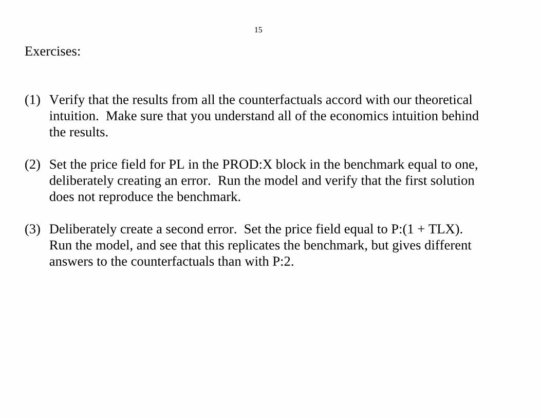
Exercises:
(1) Verify that the results from all the counterfactuals accord with our theoreticalintuition. Make sure that you understand all of the economics intuition behindthe results.
(2) Set the price field for PL in the PROD:X block in the benchmark equal to one,deliberately creating an error. Run the model and verify that the first solutiondoes not reproduce the benchmark.
(3) Deliberately create a second error. Set the price field equal to P:(1 + TLX). Run the model, and see that this replicates the benchmark, but gives differentanswers to the counterfactuals than with P:2.
16
Model 32 Labor supply and labor tax
This model is an extension of the previous model and also extends our earlier modelwith endogenous labor supply (M26) to a case with taxes in the benchmark.
Since the extension here is fairly straightforward, we will take the opportunity tointroduce two useful features. One is to first run the model without allowing it to iterate. This allows the modeler to check if the initial values of the model are an equilibrium; thatis, is it calibrated correctly? If it is not calibrated correctly, it will indicate what activitiesor markets are out of balance which is very useful in correcting the calibration.
Second, when the modeler wants to loop over a set of parameter values repeatedlysolving the model, there is a simple procedure for doing this.
There are supply activities for labor (TL) and capital (TK). Labor can also be used forleisure and so the activity level for labor supply will vary. Capital has no alternative useso it will always be completely supplied to the market. Still, it can be convenient tospecify a supply activity, since the tax on capital supply need only be specified once andthere will be two prices, one the consumer price and one the producer price (user cost) of
18
capital.
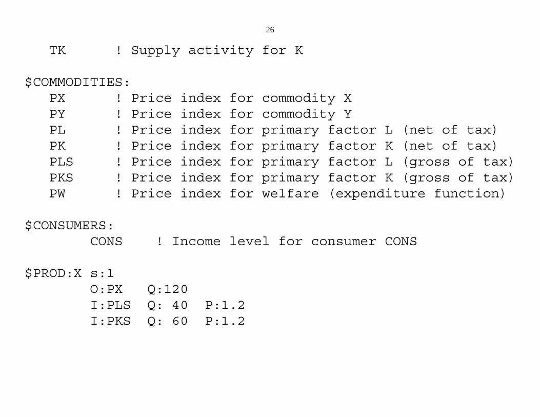
As in the previous model, we have to make a choice of units for prices. Our choicewill be that the consumer prices (prices received by the consumer) for labor and capitalwill be set to one. The data matrix indicates that there is a 20% tax on each factor in thebenchmark, so the producer prices (user costs) of labor and capital will be PLS = PKS =1.2.
We can also choose how to interpret the X and Y values, but there is only a singleprice for both producers and consumers, so we will interpret these as 120 units at a priceof 1 for each. From here on, things are rather straightforward, so let us introduce acouple of other useful features.
First, in complicated models with lots of sectors and taxes, benchmarking is adifficult task and it is often not possible to calibrate the model with all prices and activitylevels equal to one. One useful trick for checking the calibration and noting whichsectors or markets are out of balance is to not allow the model to iterate initially. Afterthe MPS/GE model itself, you will see the notation:
PLS.L =1.2; PKS.L =1.2;
19
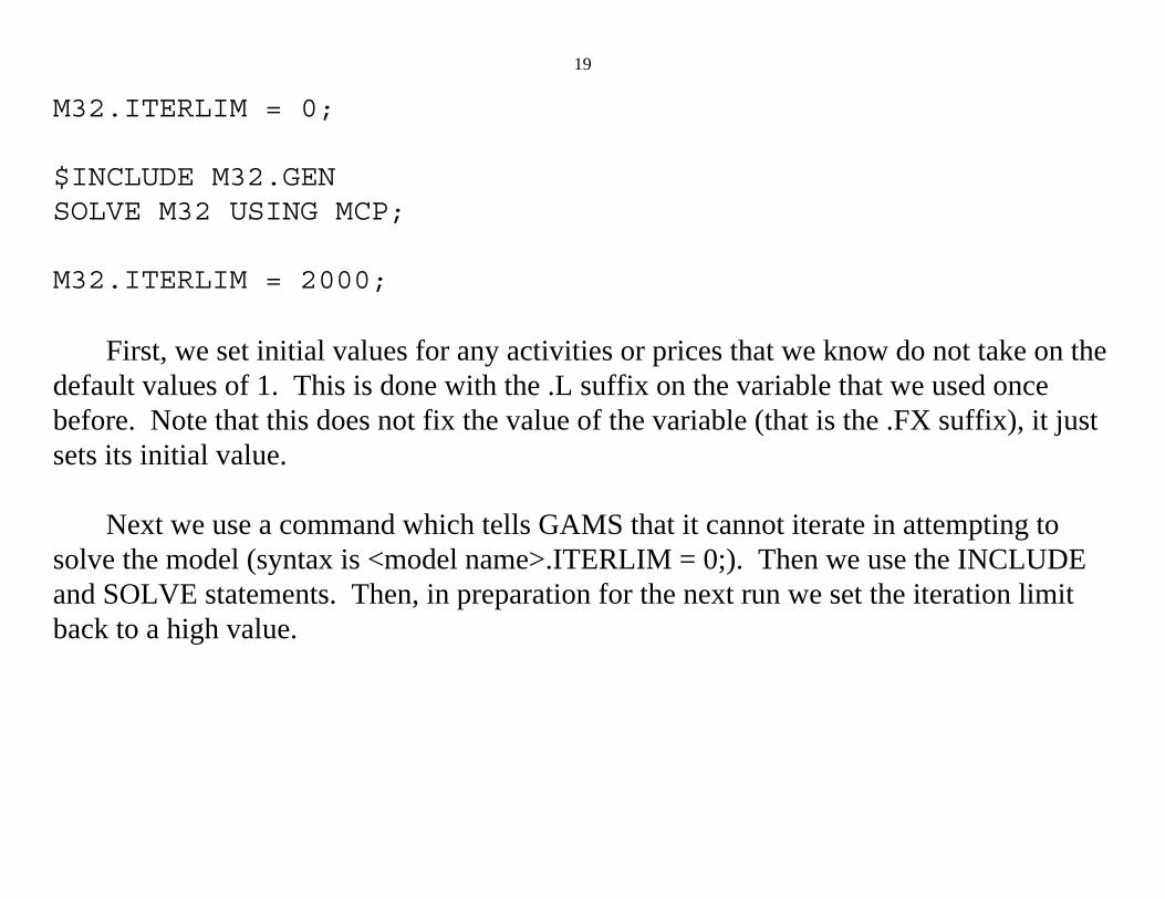
M32.ITERLIM = 0;
$INCLUDE M32.GENSOLVE M32 USING MCP;
M32.ITERLIM = 2000;
First, we set initial values for any activities or prices that we know do not take on thedefault values of 1. This is done with the .L suffix on the variable that we used oncebefore. Note that this does not fix the value of the variable (that is the .FX suffix), it justsets its initial value.
Next we use a command which tells GAMS that it cannot iterate in attempting tosolve the model (syntax is <model name>.ITERLIM = 0;). Then we use the INCLUDEand SOLVE statements. Then, in preparation for the next run we set the iteration limitback to a high value.
20
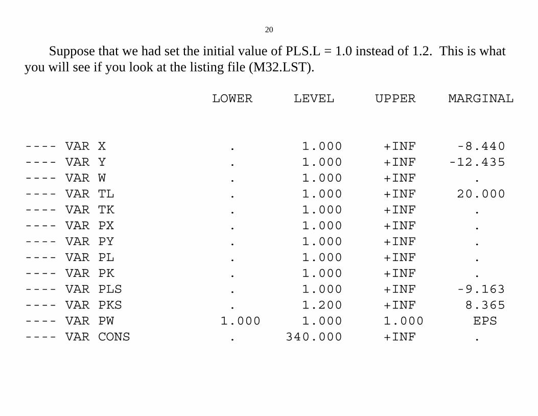
Suppose that we had set the initial value of PLS.L = 1.0 instead of 1.2. This is whatyou will see if you look at the listing file (M32.LST).
LOWER LEVEL UPPER MARGINAL
---- VAR X . 1.000 +INF -8.440 ---- VAR Y . 1.000 +INF -12.435 ---- VAR W . 1.000 +INF . ---- VAR TL . 1.000 +INF 20.000 ---- VAR TK . 1.000 +INF . ---- VAR PX . 1.000 +INF . ---- VAR PY . 1.000 +INF . ---- VAR PL . 1.000 +INF . ---- VAR PK . 1.000 +INF . ---- VAR PLS . 1.000 +INF -9.163 ---- VAR PKS . 1.200 +INF 8.365 ---- VAR PW 1.000 1.000 1.000 EPS ---- VAR CONS . 340.000 +INF .
21
The model has not solved. Recall from chapter 1 that GAMS writes inequalities in thegreater-than-or-equal-to format.
The MARGINAL column of the listing file gives the degree of imbalance in aninequality, left-hand side minus right-hand side. A positive number is ok if theassociated variable is zero, as in a cost equation (marginal cost minus price is positive ifassociated with a slack activity). A negative value of a marginal cannot be anequilibrium; for an activity it indicates positive profits and for a market it indicatesdemand exceeds supply.
In our incorrect calibration in which we give the producer price of labor too low avalue, we see that there are positive profits for X , Y and negative profits for laborsupply. There is an excess demand for labor and an excess supply for capital.
Most calibration errors are in the MPS/GE file itself, and not just in setting the initialvalues of the variables. You could work with this file as an exercise, deliberatelyintroducing errors (such as in the price fields) and see what happens. In any case, theiterlim = 0 statement is very useful in helping you identify where the errors are.
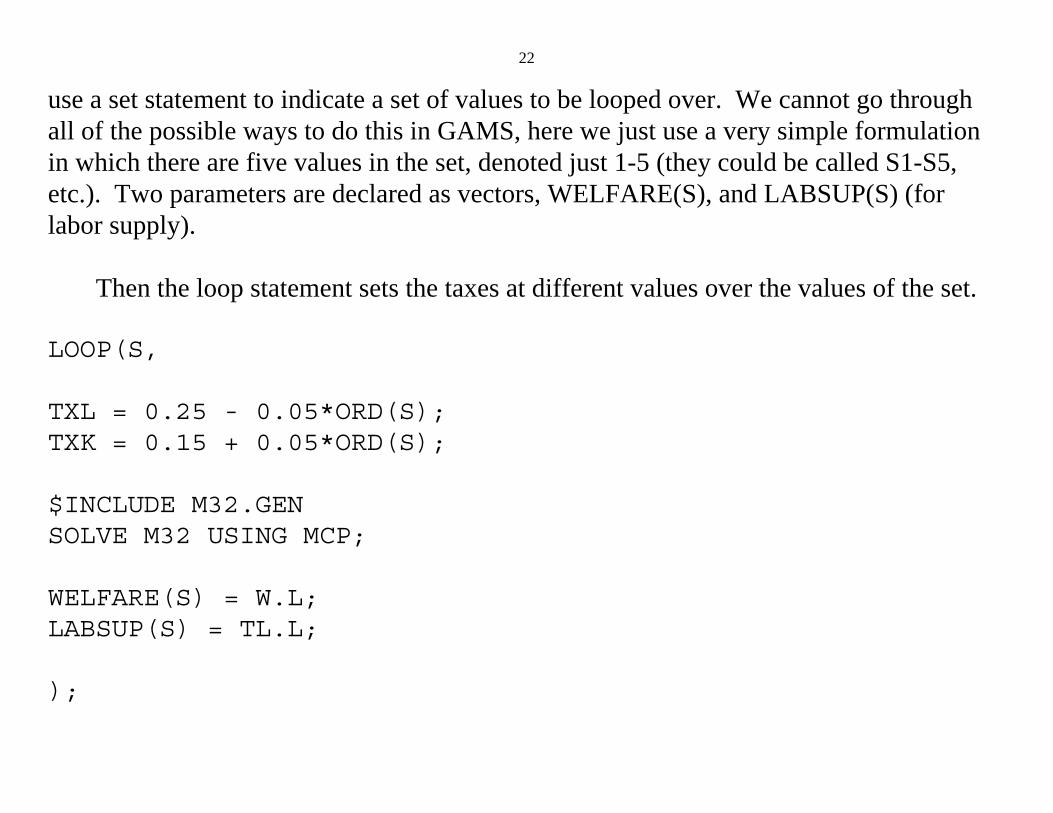
The other useful feature we introduce in this model is the use of the LOOP statementto simplify the repeated solving of the model over a series of parameter values. First, we
22
use a set statement to indicate a set of values to be looped over. We cannot go throughall of the possible ways to do this in GAMS, here we just use a very simple formulationin which there are five values in the set, denoted just 1-5 (they could be called S1-S5,etc.). Two parameters are declared as vectors, WELFARE(S), and LABSUP(S) (forlabor supply).
Then the loop statement sets the taxes at different values over the values of the set.
ORD(S) denotes the ordinal value of a member of a set. S is an indicator and is nottreated as a number in GAMS, so 0.05*S won’t work. ORD(S) is treated as a number, sothis is how the set index is translated into a number. Note from the tax assignmentstatement that when S = 1, the initial values of both taxes are 0.20, our benchmark values. At S = 5, the values are TXL = 0, and TXK = 0.40.
The model is repeatedly solved within the loop, and after each solve statement thevalue of the parameters WELFARE and LABSUP are assigned values. The loop isclosed with “ ); ” After the loop is closed we ask GAMS to display the parameters at theend of the listing file. Note the set index for the parameters is not used in the displaystatement, GAMS knows what it is.
24
$TITLE Model M32: Closed 2x2 Economy -- income taxes and*labor supply
* Declare parameters to be used in setting up* counter-factual equilibria:
SETS S /1*5/;
PARAMETERS TXL Labor income tax rate, TXK Capital income tax rate, WELFARE(S) Welfare, LABSUP(S) Labor supply;
$ONTEXT
$MODEL:M32
$SECTORS: X ! Activity level for sector X Y ! Activity level for sector Y W ! Activity level for sector W (welfare index) TL ! Supply activity for L
26
TK ! Supply activity for K
$COMMODITIES: PX ! Price index for commodity X PY ! Price index for commodity Y PL ! Price index for primary factor L (net of tax) PK ! Price index for primary factor K (net of tax) PLS ! Price index for primary factor L (gross of tax) PKS ! Price index for primary factor K (gross of tax) PW ! Price index for welfare (expenditure function)
(1) As suggested above in M31, deliberately create the same calibration errors in theMPS/GE file and see how this affects the attempt to reproduce the benchmark datausing the iterlim = 0 statement.
(2) Change the elasticity of substitution between leisure and goods from 0.7 to 0.5. Seeif you can guess how this should effect the results from the counter-factuals. Shouldthe shift to capital taxation increase welfare faster or not?
(3) In order to get more comfortable with setting producer versus consumer prices,reinterpret the bencmark data so that the producer prices (user costs) of capital andlabor are equal to one. So, for example, the value of labor in the X sector of 48 is 48units at a price of 1. Rewrite the MPS/GE file using this convention.
31
Model 33 Equal yield tax reform
This model is a follow-up on model M32 where we considered some income taxreform experiments. Like that model, here we apply taxes through activities whichtransform (supply) household owned factors into production inputs. The difference hereis that we set up a model in which we can do differential tax policy analysis holding thelevel of government revenue constant. In order to keep things simple, we continue torebate tax revenue in lump-sum fashion.
This model introduces a fourth (and final) class of MPSGE variables (in addition toactivity levels, commodity prices and income levels). The new entity is called an"auxiliary variable". In this model, we use an auxiliary variable to endogenously alter thetax rate in order to maintain an equal yield.
In the present case, we will hold the labor tax rate exogenous, but change its value,in each case solving for the value of the capital tax that yields the same value of revenueas the original tax. TXK now become a variable, not a parameter. In the initial MPS/GEstatements specifying the model, we declare a list of “auxiliary variables” (note thespelling of auxiliary, use a double “l” and the model will crash), in this case a singlevariable TXK.
32
$AUXILIARY: TXK ! Endogenous capital tax from equal yield constraint.
This variable appears in the production block for capital supply as follows.
N: is a new field in a production block, standing for eNdogenous tax rate followed by theauxiliary variable. This is read in words as “assign to consumer CONS the revenue froman endogenous tax rate TXK”. TXK is in turn associated with a constraint equation,which is written in GAMS syntax but inside the MPS/GE block. Here is how we write itin this model.
The left-hand side is tax revenue from the two taxes, one an exogenous parameter (TXL)and the other an endogenous variable (TXK). Each term is (tax rate) x (factor price) x(activity level for factor supply) x (the reference quantity supplied at an activity level
33
equal to one).
The right-hand side of the constraint specifies the target revenue. With priceschanging in general equilibrium, the modeler has to think carefully about what is meantby “constant” revenue: that is, constant in terms of what?
Here we assume that the government wants the taxes to yield an amount equal to thecost of purchasing given and equal amounts of X and Y, so for example the initial taxrevenue of 40 is spend (at prices for X and Y equal to one) on 20 X and 20 Y.
The right-hand side of the constraint equation will continue to allow the purchase of X = Y = 20 as the prices of the goods change in general equilibrium.
Of course, the government is not actually buying anything in this simple model, it isjust redistributing the revenue back to the consumer. But the point is that the modelermust specify what the revenue target is in real terms, and then allow the nominal value ofthat to adjust with prices.
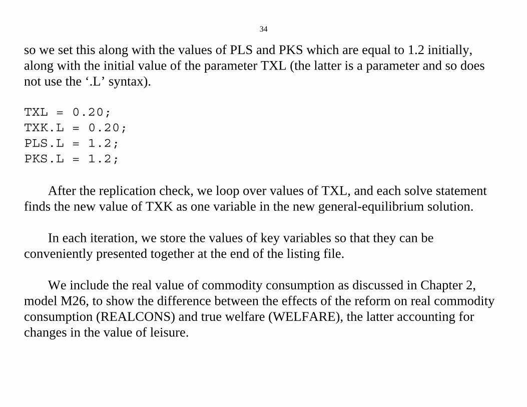
For historical reasons, the default values of auxiliary variables in MPS/GE are zero,not one. So the modeler should set the initial values of these variables for the replicationcheck even if they should happen to be one. In our case, the initial value of TXK = 0.20,
34
so we set this along with the values of PLS and PKS which are equal to 1.2 initially,along with the initial value of the parameter TXL (the latter is a parameter and so doesnot use the ‘.L’ syntax).
TXL = 0.20;TXK.L = 0.20;PLS.L = 1.2;PKS.L = 1.2;
After the replication check, we loop over values of TXL, and each solve statementfinds the new value of TXK as one variable in the new general-equilibrium solution.
In each iteration, we store the values of key variables so that they can beconveniently presented together at the end of the listing file.
We include the real value of commodity consumption as discussed in Chapter 2,model M26, to show the difference between the effects of the reform on real commodityconsumption (REALCONS) and true welfare (WELFARE), the latter accounting forchanges in the value of leisure.
35
Note from the results in the present case, that measuring only the change in realcommodity consumption significantly overstates the true welfare gain of the tax reform(which is tiny) because of the fall in leisure (increase in labor supply).
Finally, although the difference is small, note that the capital tax that needs to beassociated with TXL = 0 is TXK = 0.476, not the 0.50 value we assumed in the previousmodel adjusting the capital and labor taxes one for one in opposite directions.
36
$TITLE Model M33: Closed 2x2 Economy -- Equal Yield Tax*Reform
PARAMETERS TXL Labor income tax rate, WELFARE(S) Welfare, REALCONS(S) Real consumption of goods, LABSUP(S) Labor supply, CAPTAX(S) Capital tax rate; $ONTEXT
$MODEL:M33
$SECTORS: X ! Activity level for sector X Y ! Activity level for sector Y W ! Activity level for sector W (welfare index) TL ! Supply activity for L TK ! Supply activity for K
38
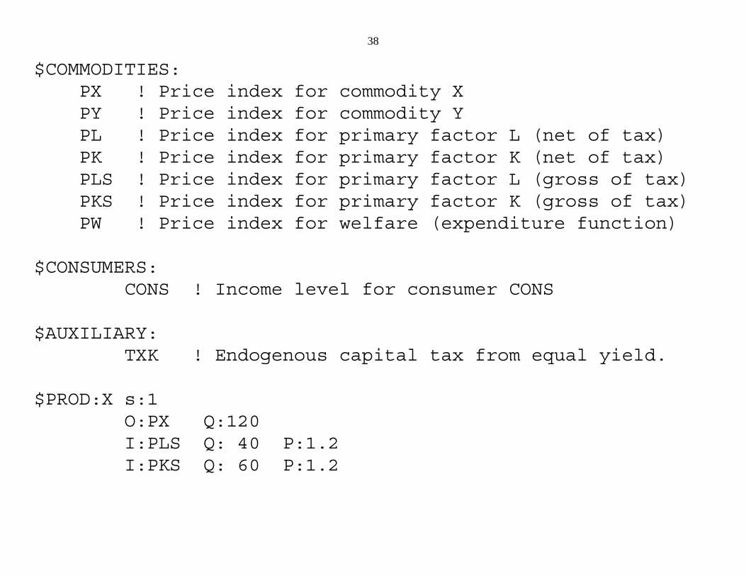
$COMMODITIES: PX ! Price index for commodity X PY ! Price index for commodity Y PL ! Price index for primary factor L (net of tax) PK ! Price index for primary factor K (net of tax) PLS ! Price index for primary factor L (gross of tax) PKS ! Price index for primary factor K (gross of tax) PW ! Price index for welfare (expenditure function)
$CONSUMERS: CONS ! Income level for consumer CONS
$AUXILIARY: TXK ! Endogenous capital tax from equal yield.
The assumption of lump-sum redistribution is a convenient trick which simplifies taxpolicy analysis. In practice, governments often use money to purchase things whichprivate markets do not provide. People value the public provision, but for some reason itis not easy to collect money from beneficiaries.
In this model, we first explicitly introduce government as an agent or “consumer”(GOVT). The tax revenue collected in the economy is assigned to the government. Thegovernment spends this on purchasing a good called G (price PG), which is producedfrom capital and labor like the other goods X and Y. Here is the production block for G(all inputs in all sectors are taxed at 25%) and the demand block for the consumer GOVT.
The government is the only agent demanding PG in the model. As we noted back inChapter 1, MPS/GE transfers the tax revenue to the government in the background, thisbeing the government’s only source of income.
Now comes the tricky part. Each consumer receives the full benefit of the publicgood without actually purchasing or paying for it. The community park is just there, freefor the consumer. How do we model this free transfer from the government to theconsumer?
To do this, we introduce another feature of MPS/GE, the rationing variable andrationing constraint. The rationing variable is declared as an auxiliary variable, denotedhere LGP It appears as a multiplier on an endowment field in a consumer’s demandequation. Here is the correct syntax for the demand blocks for the two consumers.
MPS/GE just multiplies the quantity in the Q field by the value of the variable in the Rfield, so in this case CONS1 has an endowment of PG1 equal to 50*LGP.
The value of LGP, like any auxiliary variable is set by a constraint equation. In ourcase, LGP takes on the value of G, the activity level for production of the public good. Note that 50 is the reference quantity for the G activity at G = 1, so the auxiliaryrationing variable LGP transfers the full amount of the public good to each consumer.
$CONSTRAINT:LGP LGP =E= G;
Note that we have defined and used two different commodities for the public goodendowments of the two consumers, PG1 and PG2 respectively, even though eachconsumer is getting the full (and therefore equal) amount of the public good. The reasonthat we do this is to prevent the consumers from being able to trade the goods in the event
45
that they have different valuations of public good.These “personalized” endowments ofthe public good are then inputs to each consumer’s welfare.
Only consumer 1 is endowed wit PG1 and only consumer 1 demands PG1. Similarcomments apply to consumer 2 and PG2.
What about the valuations of the public goods at a price PG1 = PG2 = 0.5? We aregoing to assume that the initial data represent an optimal initial provision of the publicgood. According to the Samuelson rule, discussed in connection with the next model, the
46
public good is optimally provided with non-distortionary taxation if the cost of providingone unit equals the sum of the demand prices, since each consumer consumes the fullamount. This is satisfied here if each consumer has a demand price of 0.5 in the initialbenchmark situation.
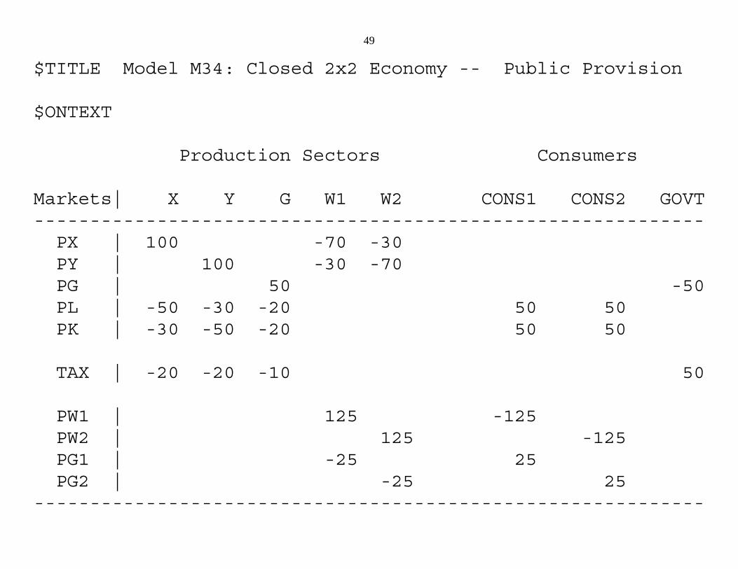
Now we will give the full micro-consistent data matrix for this problem. Factorsupplies are taxes at 25% to all sectors.
The government is treated as another consumer, with an income balance conditionthat the GOVT column sum is zero. Taxes are treated like a market subject to a zero-row-sum, market-clearing condition: all tax revenues generated must be assigned tosomething. The personalized public goods are endowments of the consumers and inputs
48
into consumers’ welfare functions.
Take some time working through the rows and columns of this matrix. Note the zerorow and column sums, and make sure that you understand each one.
Note finally that this data matrix is somewhat different from those used previous inthat some of these entries are valuations are not observed in the market data (this wasalso true of the labor/leisure models, where the endowment of leisure and its valuation isnot directly observed). The last four rows of the matrix are not observed in market data. We have constructed them under the assumptions that (a) the consumers have identicalpreferences for the public good, (b) the benchmark data represents a optimal provision ofthe public good.
Now we present the full model using these data. Note the specification of the initialvalues of variables not equal to one and the value of the auxiliary variable (default iszero, not 1) prior to the replication check (iterlim = 0).
49
$TITLE Model M34: Closed 2x2 Economy -- Public Provision
PARAMETERS TAX Tax rate on factor inputs to all sectors;
$ONTEXT
$MODEL:M34
$SECTORS: X ! Activity level for sector X Y ! Activity level for sector Y G ! Activity level for sector G (public provision) W1 ! Activity level for sector W1 (cons 1 welfare index) W2 ! Activity level for sector W2 (cons 2 welfare index)
51
$COMMODITIES: PX ! Price index for commodity X PY ! Price index for commodity Y PG ! Price index for commodity G(cost of public output) PL ! Price index for primary factor L (net of tax) PK ! Price index for primary factor K PW1 ! Price index for welfare (consumer 1) PW2 ! Price index for welfare (consumer 2) PG1 ! Private valuation of the public good (consumer 1) PG2 ! Private valuation of the public good (consumer 2)
M34.ITERLIM = 0;$INCLUDE M34.GENSOLVE M34 USING MCP;
M34.ITERLIM = 2000;
* The following counterfactuals check that the original* benchmark is indeed an optimum by raising/lowering the* tax
55
TAX = 0.20;
$INCLUDE M34.GENSOLVE M34 USING MCP;
TAX = 0.30;
$INCLUDE M34.GENSOLVE M34 USING MCP;
56
Exercises:
(1) Define a set, parameters, and write a loop statement over finer values of the tax rate(e.g., 1% steps) storing the welfare of each consumer for each tax rate. See if the taxof 25% is optimal.
(2) Change one consumer’s valuation of the public good. The first run of the modelshould reproduce the benchmark data, but one consumer will prefer a different taxrate. Conduct the same experiment as in (1) with the new valuation and see whathappens from the point of view of each consumer.
57
Model 35 Public good tax rate set endogenously by Samuelson rule
This model is exactly the same as the previous one, except that the tax used tofinance the public good is endogenous. Thus we will not repeat the data matrix here, andmost other elements of the model are already familiar.
Instead of TAX being a parameter, it is now an auxiliary variable. Its value is set bythe constraint equation:
$CONSTRAINT:TAX PG =E= PG1 + PG2;
This is a condition noted by Samuelson many years ago. Since each consumer getsthe full amount of the public good (the good is “non-rivaled”), the marginal benefit ofanother unit of the good is the sum of the demand prices for all the consumers. Efficiency is achieved when this sum of benefits is equal to the marginal cost ofproducing another unit. This is given by the above equation.
Note that the auxiliary variable itself need not appear in the constraint equationassociated with it. The solution algorithm will adjust TAX in order to satisfy thiscondition.
58
Strictly speaking, the Samuelson rule is valid only if the tax needed to pay for thepublic good can be raised in a non-distortionary way. If distortionary taxes must be used,the sum of marginal benefits must be weighed against the marginal cost of productionplus the marginal burden of taxation. It is beyond the scope of this chapter to discuss thisproblem further here.
When we run this model, we will get back a value of TAX = 0.25, because wecalibrated the prefences assuming that the initial data was optimal. As a counterfactualexperiment, we change one consumer’s valuation of the public good, using a parameterVG1 which is a multiplier on consumer 1's initial valuation of the good.
In the counterfactual experiment we double consumer 1's “willingness to pay”,setting VG1 = 2. Here are some results from the counterfactual.
59
---- VAR X . 0.909 +INF . ---- VAR Y . 0.909 +INF . ---- VAR G . 1.364 +INF . ---- VAR W1 . 1.041 +INF . ---- VAR W2 . 0.986 +INF . ---- VAR TAX . 0.375 +INF .
With consumer 1's increased valuation of the public good, it is optimal to raise thetax from 0.25 to 0.375 as shown. Resources are transferred out of producing final goodsX and Y and into producing G. The activity for G rises from 1.0 in the benchmark to1.364.
Note that, although the high tax is efficient according to the Samuelson rule, itnevertheless results in a redistribution of welfare from the low valuation consumer to thehigh valuation consumer.
There are many uses for the type of modeling in public and environmentaleconomics. Environmental economists in particular devote large amounts of effort tosoliciting individuals’ preferences for non-market goods. The results of such surveys andstudies can serve as inputs into calibrating the preferences for models such as this one.
60
When calibrated, it is unlikely that the initial level of public goods (or environmentalquality) is optimal. The following program can then be used to find what the optimumlevel and optimal taxes are.
61
$TITLE Model M35: Closed 2x2 Economy - Public Output with*Samuelson Rule
* This model is the same as M34 except that the tax to* finance the * public good is set endogenously
PARAMETER VG1 Preference index for public goods for consumer 1;
VG1 = 1;
$ONTEXT
$MODEL:M35
$SECTORS: X ! Activity level for sector X Y ! Activity level for sector Y G ! Activity level for sector G (public provision) W1 ! Activity level for sector W1 (consumer 1 welfare)
62
W2 ! Activity level for sector W2 (consumer 2 welfare)
$COMMODITIES: PX ! Price index for commodity X PY ! Price index for commodity Y PG ! Price index for commodity G (marg cost of pub out) PL ! Price index for primary factor L (net of tax) PK ! Price index for primary factor K PW1 ! Price index for welfare (consumer 1) PW2 ! Price index for welfare (consumer 2) PG1 ! Private valuation of the public good (consumer 1) PG2 ! Private valuation of the public good (consumer 2)
M35.ITERLIM = 0;$INCLUDE M35.GENSOLVE M35 USING MCP;
M35.ITERLIM = 2000;
* What happens to consumer 2 welfare if consumer 1* decides* she would like more public output:
VG1 = 2;
$INCLUDE M35.GENSOLVE M35 USING MCP;
Exercise:
Run this counterfactual again, except fix the tax rate at its initial optimal value: TAX.L =0.25. See how this changes the welfare of the two consumers.
67
Model 36 Taxes and classical unemployment
In many situations, initial data or the questions that a modeler may wish to analyzedo not correspond to an equilibrium with all markets clearing. Unemployment is anobvious situation. While MPS/GE is designed to compute equilibria with marketsclearing, there are some simple tricks to incorporate a rich set of situations and policyoptions into a model.
This model considers “classical” unemployment, by which we will simply mean thatthere is a wage which is rigid downward, perhaps a legal minimum wage. This constraintmay or may not be binding in equilibrium, and the complementarity features of GAMSand MPS/GE make this easy to compute. Other situations that the technique applies toinclude the analysis of quotas, which we will examine in the next chapter.
The model we use here is essentially the same as the one we used in M21, where weconsidered tax reform as a counterfactual experiment. The data matrix shown below isthe same one used in M21, except here we specify the total endowment of labor as 100units, but an initial unemployment rate of 20% limits the amount of labor used in X andY to 80 units. The parameter U0 is thus set at 0.20 initially. As was the case in M21, weassume that there is initially a tax of 100% on the labor used in the production of X. Theconsumer (supply) price of labor is chosen to be one, so the producer price (user cost) is
68
2, and this must appear in the price field for the X production block.
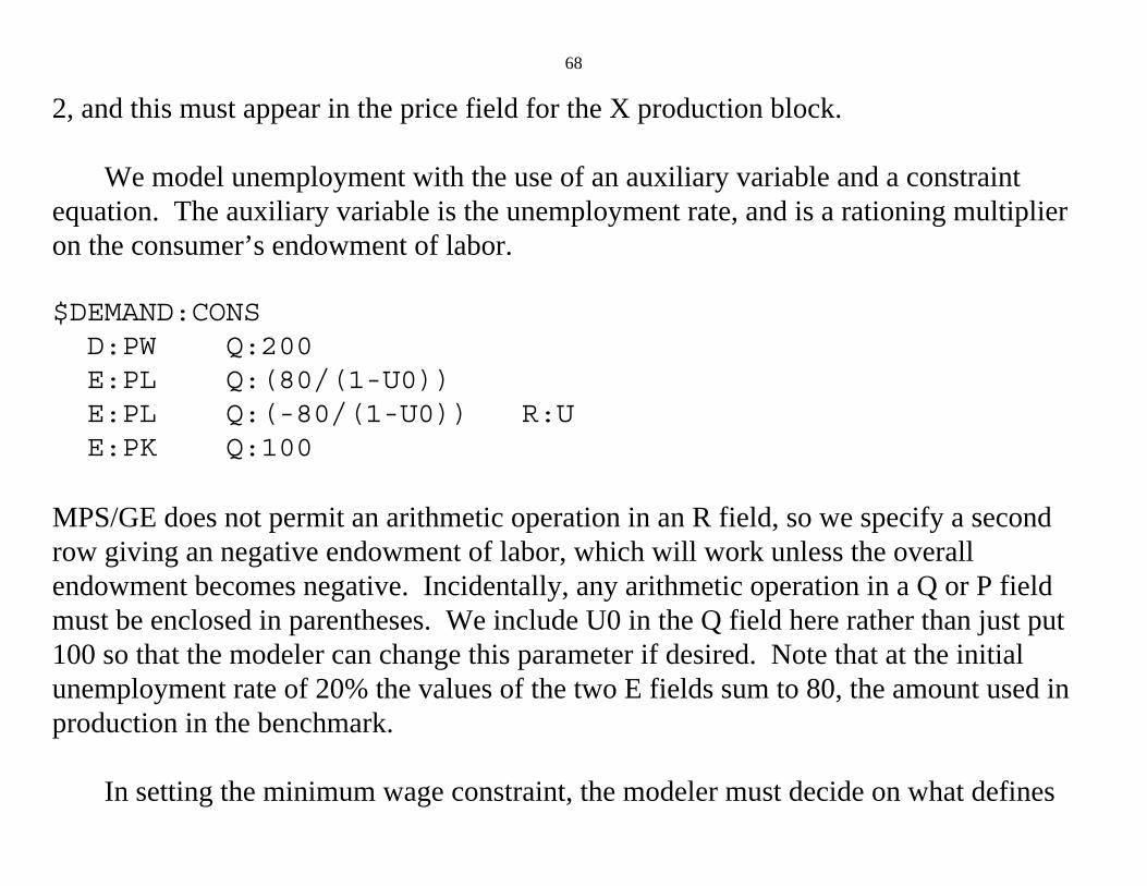
We model unemployment with the use of an auxiliary variable and a constraintequation. The auxiliary variable is the unemployment rate, and is a rationing multiplieron the consumer’s endowment of labor.
MPS/GE does not permit an arithmetic operation in an R field, so we specify a secondrow giving an negative endowment of labor, which will work unless the overallendowment becomes negative. Incidentally, any arithmetic operation in a Q or P fieldmust be enclosed in parentheses. We include U0 in the Q field here rather than just put100 so that the modeler can change this parameter if desired. Note that at the initialunemployment rate of 20% the values of the two E fields sum to 80, the amount used inproduction in the benchmark.
In setting the minimum wage constraint, the modeler must decide on what defines
69
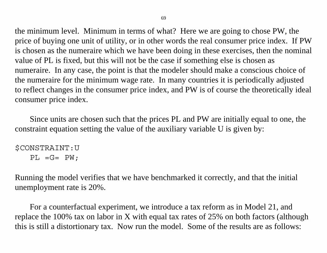
the minimum level. Minimum in terms of what? Here we are going to chose PW, theprice of buying one unit of utility, or in other words the real consumer price index. If PWis chosen as the numeraire which we have been doing in these exercises, then the nominalvalue of PL is fixed, but this will not be the case if something else is chosen asnumeraire. In any case, the point is that the modeler should make a conscious choice ofthe numeraire for the minimum wage rate. In many countries it is periodically adjustedto reflect changes in the consumer price index, and PW is of course the theoretically idealconsumer price index.
Since units are chosen such that the prices PL and PW are initially equal to one, theconstraint equation setting the value of the auxiliary variable U is given by:
$CONSTRAINT:UPL =G= PW;
Running the model verifies that we have benchmarked it correctly, and that the initialunemployment rate is 20%.
For a counterfactual experiment, we introduce a tax reform as in Model 21, andreplace the 100% tax on labor in X with equal tax rates of 25% on both factors (althoughthis is still a distortionary tax. Now run the model. Some of the results are as follows:
70
LOWER LEVEL UPPER MARGINAL
---- VAR X . 1.178 +INF ---- VAR Y . 1.106 +INF ---- VAR W . 1.142 +INF ---- VAR PX . 0.969 +INF ---- VAR PY . 1.032 +INF ---- VAR PL . 1.051 +INF ---- VAR PK . 1.005 +INF ---- VAR PW 1.000 1.000 1.000 EPS ---- VAR CONS . 228.374 +INF . ---- VAR U . . +INF 0.051
The minimum wage ceases to be binding (PL = 1.051) and unemployment falls tozero (note that the marginal on U is the excess of PL over PW). There is a very largeincrease in welfare, which goes to 1.142 as the increases in employment reinforces thetax reform.
71
There are some very interesting policy economics in this example. Initially, we havetwo distortions that are reinforcing one another. If we reform the tax structure, thesecond distortion is automatically removed by making it non-binding.
To see this effect, we do one final counterfactual in the model, which is to fix theunemployment rate at its initial value of 20%, but allow the tax reform. If you look at thelisting file, you will see that welfare rises to only 1.021.
Most of the effect of the tax reform shown above is its indirect effect in eliminatingthe binding minimum wage constraint.
72
$TITLE Model M36: Closed 2x2 Economy - Taxes and ClassicalUnemployment
PARAMETERS TX Proportional output tax on sector X, TY Proportional output tax on sector Y, TLX Ad-valorem tax on labor inputs to X,
73
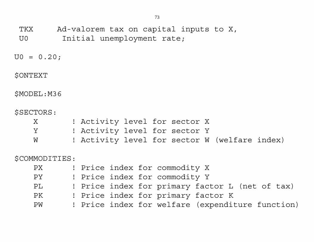
TKX Ad-valorem tax on capital inputs to X, U0 Initial unemployment rate;
U0 = 0.20;
$ONTEXT
$MODEL:M36
$SECTORS: X ! Activity level for sector X Y ! Activity level for sector Y W ! Activity level for sector W (welfare index)
$COMMODITIES: PX ! Price index for commodity X PY ! Price index for commodity Y PL ! Price index for primary factor L (net of tax) PK ! Price index for primary factor K PW ! Price index for welfare (expenditure function)
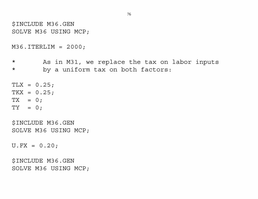
* As in M31, we replace the tax on labor inputs* by a uniform tax on both factors:
TLX = 0.25; TKX = 0.25;TX = 0;TY = 0;
$INCLUDE M36.GENSOLVE M36 USING MCP;
U.FX = 0.20;
$INCLUDE M36.GENSOLVE M36 USING MCP;
77
Exercises:
(1) Try a different numeraire for defining the minimum wage and see what happens.
(2) If you want to be a little bit more ambitious, try adding a labor-leisure decision to theproblem.
78
Model 37 Steady-state capital stock
As in the case of labor supply, we would like to have models in which the stock ofcapital is endogenous. This requires dynamic modeling, a significant complication ofwhat we have done to this point. This chapter will not consider true dynamic modeling. However, we will present a shortcut that is very valuable in many situations. In modelsfor which there exists a steady state, it is possible to represent this steady state as acomplementarity problem not that different from our static models. We can then at leastperform comparative steady-state experiments, in which a parameter change moves usfrom one steady state to another. But actually solving for the transition path requires amore complicated analysis that is postponed until later in the book.
Model 37 incorporates optimal capital accumulation via the use of a rationingconstraint and endogenous “taxes” to create a model for comparative steady state analysiswhen the capital stock is endogenously adjusted to its steady-state value. The labor forceis assumed fixed in this model.
Let r denote the rental price (for one period) of a unit of capital and let pk denote theprice of a new unit of capital. * will denote the rate of depreciation of capital per period,and D will denote the discount rate between periods. The steady-state optimal capitalaccumulation condition is a relationship between the price and rental rate on capital. The
79
rental rate must be given by:
The rental price (r) is equal to the price of creating a new unit of capital (pk) minus thepresent value of what the capital could be sold for next period. In the steady state, theprice of a new unit next period is the same, so an old unit can be sold for its originalvalue minus one period’s depreciation (1 - *). The present value of the undepreciatedportion is thus (1 - *)/(1+ D).
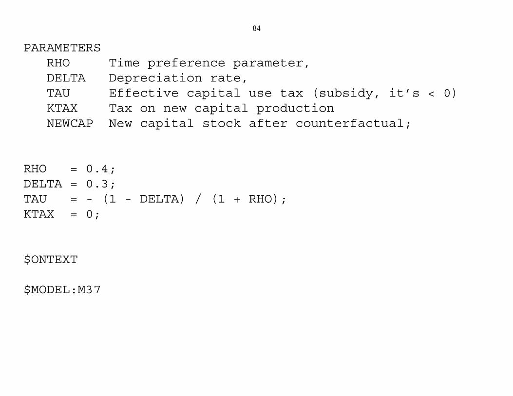
The dynamic steady-state problem is represented as a static problem using twotricks. First, the use of capital is subsidized to create the desired wedge (denoted TAU)between the rental price and the price of new capital. Following the declaration of theparameters DELTA, RHO, and TAU you will see:
TAU = - (1 - DELTA) / (1 + RHO);
80
This then appears as a subsidy to capital use, creating the wedge between the rental priceand the price of producing a new unit of capital (PK).
One unit of new capital is produced using one unit of labor, as you will see in theproduction block for activity K.
Second, since in the steady state newly produced capital is equal to depreciation anddepreciation is equal to a share DELTA of total capital, a rationing constraint is specifiedto "endow" consumers with the carryforward from the previous period. Let Ks denote thecapital stock and Kn the production of new capital. In the steady state, these are related
81
by:
The carryforward from the previous period is the steady state stock minus newproduction. It is is called KFORWD and given by:
carry forward = KFORWD =
So in the model below, we will give the consumer an endowment, via the rationingmultiplier KFORWD, the quantity of capital on the right-hand side of the above equation.
$DEMAND:CONS D:PW E:PL Q:160 E:PK Q:1 R:KFORWRD
82
$CONSTRAINT:KFORWRD KFORWRD =E= K * (1-DELTA) / DELTA;
That completes the model description. As has been our practice, we include theinitial micro-consistent data matrix in the program. Study this carefully in going throughthe program. Note that in the data matrix, the consumer is “endowed” with 140 units ofcapital. In the program, this is the carry forward and is subject to change incounterfactual experiments.
Two counterfactuals are run in the program. First the rate of time preference D israised. In the second, D is set back to its initial value, and there is a tax on new capitalproduction. See if you can guess what the effects of these changes should be, and thenlook at the results.
83
$TITLE Model M38: Closed 2x2 Economy - Steady State CapitalStock
$ONTEXT
Production Sectors Consumers
Markets | X Y K W | CONS ------------------------------------------------------ PX | 100 -100 | PY | 100 -100 | PW | 200 | -200 PL | -40 -60 -60 | 160 PK | -120 -80 60 | 140 SUB | 60 40 | -100 ------------------------------------------------------
$OFFTEXT
84
PARAMETERS RHO Time preference parameter, DELTA Depreciation rate, TAU Effective capital use tax (subsidy, it’s < 0) KTAX Tax on new capital production NEWCAP New capital stock after counterfactual;
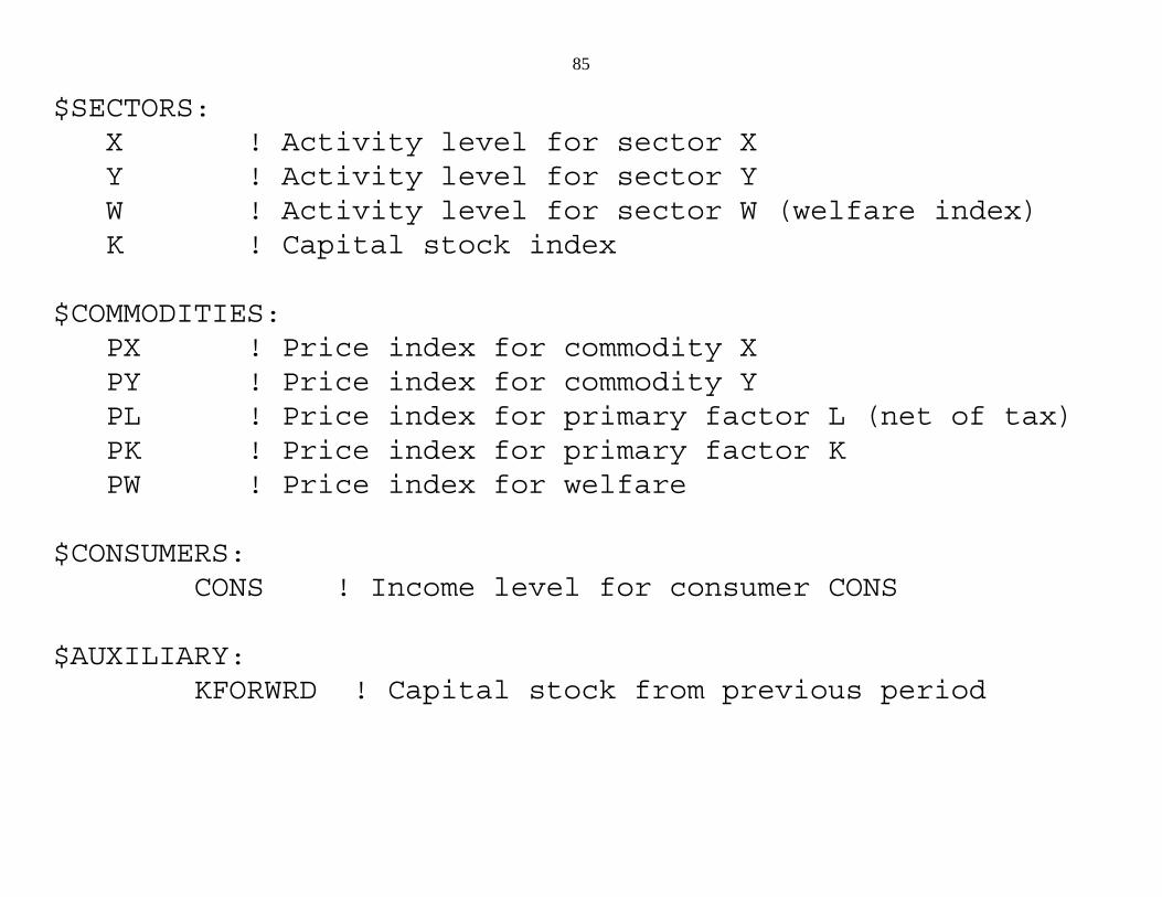
$SECTORS: X ! Activity level for sector X Y ! Activity level for sector Y W ! Activity level for sector W (welfare index) K ! Capital stock index
$COMMODITIES: PX ! Price index for commodity X PY ! Price index for commodity Y PL ! Price index for primary factor L (net of tax) PK ! Price index for primary factor K PW ! Price index for welfare
$CONSUMERS: CONS ! Income level for consumer CONS
$AUXILIARY: KFORWRD ! Capital stock from previous period
$CONSTRAINT:KFORWRD KFORWRD =E= K * (1-DELTA) / DELTA;
$OFFTEXT$SYSINCLUDE mpsgeset M37
K.L = 60;KFORWRD.L = 140;PW.FX = 1;
$INCLUDE M37.GENSOLVE M37 USING MCP;
88
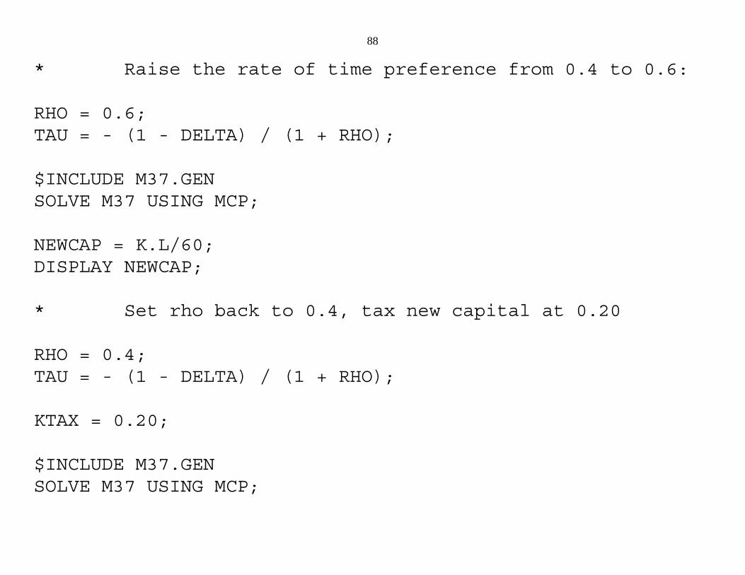
* Raise the rate of time preference from 0.4 to 0.6:
RHO = 0.6;TAU = - (1 - DELTA) / (1 + RHO);
$INCLUDE M37.GENSOLVE M37 USING MCP;
NEWCAP = K.L/60;DISPLAY NEWCAP;
* Set rho back to 0.4, tax new capital at 0.20
RHO = 0.4;TAU = - (1 - DELTA) / (1 + RHO);
KTAX = 0.20;
$INCLUDE M37.GENSOLVE M37 USING MCP;
89
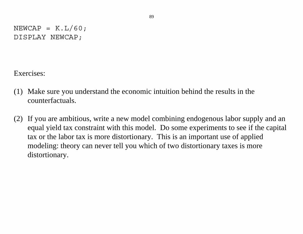
NEWCAP = K.L/60;DISPLAY NEWCAP;
Exercises:
(1) Make sure you understand the economic intuition behind the results in thecounterfactuals.
(2) If you are ambitious, write a new model combining endogenous labor supply and anequal yield tax constraint with this model. Do some experiments to see if the capitaltax or the labor tax is more distortionary. This is an important use of appliedmodeling: theory can never tell you which of two distortionary taxes is moredistortionary.