Page 1
Chapter 6. Water Quality Control
- 1 -
Chapter 4. Water Quality Control
2. Municipal Water and Wastewater Systems
FIGURE 1 Water and wastewater systems.
▶ Combined sewer systems(Sewer + Storm water)
- Collect run-off from urban streets and join sewer lines in old cities
- Overload capacity of the wastewater treatment system at heavy rainy days
- Overloaded portion must be released directly into the receiving water
▶ Complement for combined sewer system
- Prepare massive reservoirs, often underground
- Store the combined flow until the storm passes
- The reservoir is slowly drained back into the sanitary sewer system
Page 2
Chapter 6. Water Quality Control
- 2 -
3. The Safe Drinking Water Act(SDWA)
PrimaryStandards Based on health-related Enforceable
Drinkingwater
standards SecondaryStandards
Based on both aesthetics & non-aesthetic characteristics Un-enforceable
TABLE 1 Maximum Contaminant Levels(MCL, mg/L) for drinking water
Page 3
Chapter 6. Water Quality Control
- 3 -
<Secondary Standards>
TABLE 2 Secondary standards for drinking water
▶ EPA’s secondary standards
Page 4
Chapter 6. Water Quality Control
- 4 -
- Nonenforceable
- Maximum Contaminant Levels(MCL) intended to protect public welfare
- Public welfare criteria include factors such as taste, color, corrosivity, and
odor, rather than health effects.
- Some states have adopted as enforceable requirements.
▶ Effects of pollutants
- Excessive sulfate → laxative effect
- Fe and Mn → taste and their ability to stain laundry and fixtures
- Foaming and color → visually upsetting
- Excessive fluoride → a brownish discoloration of teeth
- Various dissolved gases → odor
Page 5
Chapter 6. Water Quality Control
- 5 -
4. Water Treatment Systems(or Water Treatment Plant, WTP)
▶ Purpose of WTP : treat raw water up to drinking water quality
▶ Source of raw water for drinking
Raw Water
for Drinking
GroundWater
Small TownsCommunities
focuses on removal of dissolved inorganic contaminants
SurfaceWater Large Cities focuses on particle removal by
filtration
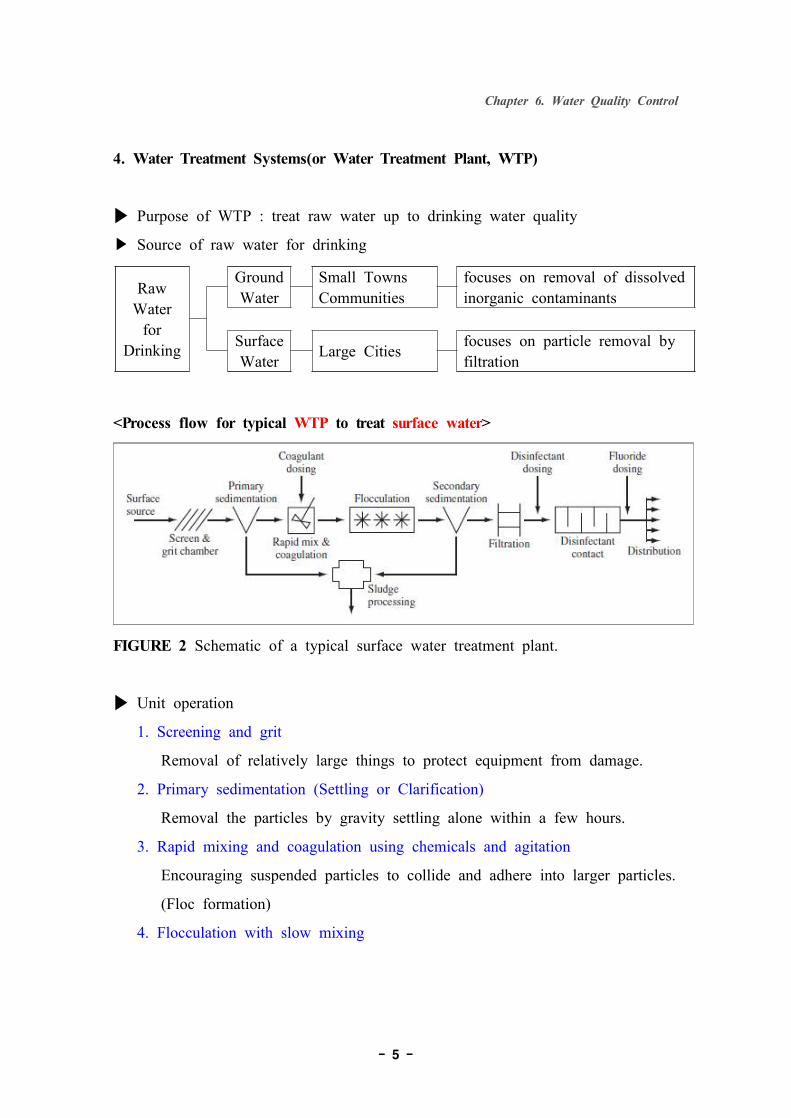
<Process flow for typical WTP to treat surface water>
FIGURE 2 Schematic of a typical surface water treatment plant.
▶ Unit operation
1. Screening and grit
Removal of relatively large things to protect equipment from damage.
2. Primary sedimentation (Settling or Clarification)
Removal the particles by gravity settling alone within a few hours.
3. Rapid mixing and coagulation using chemicals and agitation
Encouraging suspended particles to collide and adhere into larger particles.
(Floc formation)
4. Flocculation with slow mixing
Page 6
Chapter 6. Water Quality Control
- 6 -
Encouraging the formation of large particles of floc that will more easily
settle. (Enhance the floc size to be larger)
5. Secondary settling : Settling the floc slowly by Gravity.
6. Filtration
Removal of the floc that are too small or light to settle by gravity.
7. Sludge processing
Dewatering and disposing of sludge collected from the settling tanks.
8. Disinfection : Inactivating any remaining pathogens by adding disinfectant.
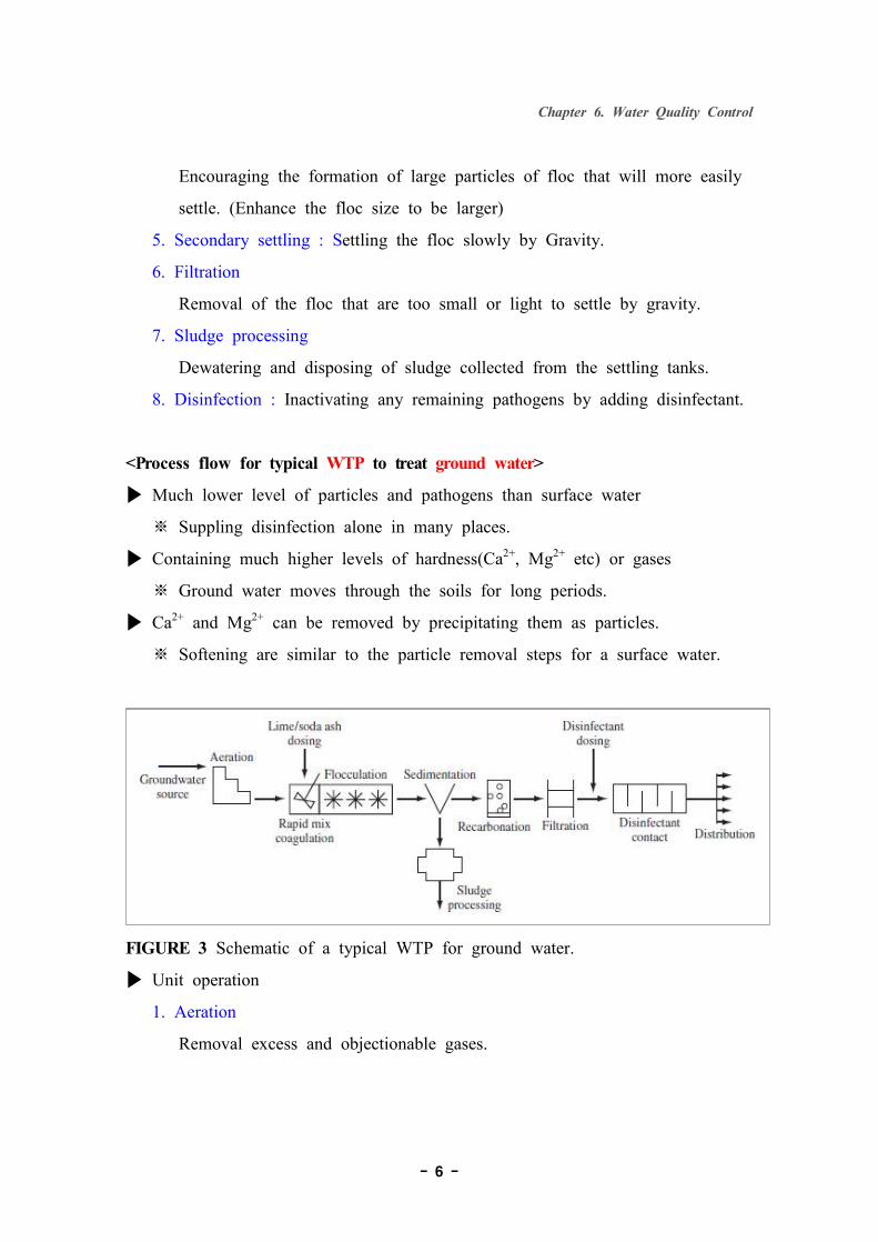
<Process flow for typical WTP to treat ground water>
▶ Much lower level of particles and pathogens than surface water
※ Suppling disinfection alone in many places.
▶ Containing much higher levels of hardness(Ca2+, Mg2+ etc) or gases
※ Ground water moves through the soils for long periods.
▶ Ca2+ and Mg2+ can be removed by precipitating them as particles.
※ Softening are similar to the particle removal steps for a surface water.
FIGURE 3 Schematic of a typical WTP for ground water.
▶ Unit operation
1. Aeration
Removal excess and objectionable gases.
Page 7
Chapter 6. Water Quality Control
- 7 -
2. Flocculation (and precipitation) follows chemical addition
Forcing Ca2+ and Mg2+ above their solubility limits. (Soluble → Solid)
3. Sedimentation
Removal the hardness particles that will now settle by gravity.
4. Re-carbonation
Re-adjusting the water pH and alkalinity.
※ Causing additional softening.
FIGURE 2-5 diagram for the carbonate system.
5. Others(filtration, disinfection, sludge processing)
Same with surface water treatment.
5.1 Sedimentation
▶ Similar Wording : Sedimentation = Clarification = Precipitation = Settling
▶ Equivalent diameter
- Hydrodynamic diameter for particles settling in water
Page 8
Chapter 6. Water Quality Control
- 8 -
- Aerodynamic diameter for particles settling in air
※ Irregular shapes of particles → equivalent diameter
(comparing them with spheres having the same settling velocity)
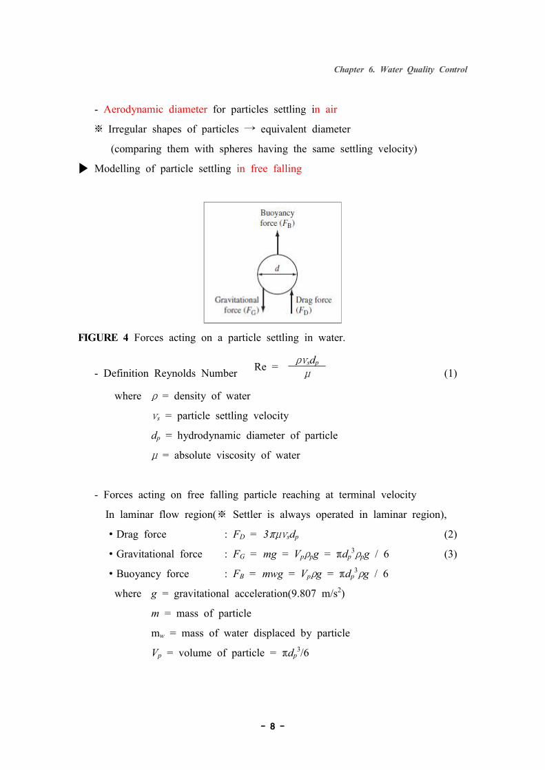
▶ Modelling of particle settling in free falling
FIGURE 4 Forces acting on a particle settling in water.
- Definition Reynolds Number Re = ρνsdp
μ (1)
where ρ = density of water
νs = particle settling velocity
dp = hydrodynamic diameter of particle
μ = absolute viscosity of water
- Forces acting on free falling particle reaching at terminal velocity
In laminar flow region(※ Settler is always operated in laminar region),
∙Drag force : FD = 3πμνsdp (2)
∙Gravitational force : FG = mg = Vpρpg = πdp3ρpg / 6 (3)
∙Buoyancy force : FB = mwg = Vpρg = πdp3ρg / 6
where g = gravitational acceleration(9.807 m/s2)
m = mass of particle
mw = mass of water displaced by particle
Vp = volume of particle = πdp3/6
Page 9
Chapter 6. Water Quality Control
- 9 -
ρp = density of particle
- Force Balance(Stock’s Law)
Gravity = Drag force(function of Re) + Buoyancy force → FG = FD + FB
FG = FD + FB → πdp3ρpg/6 = πdp
3ρg/6 + 3πμνsdp (4)
∴ Stock’s Law : νs = g(ρp - ρ)dp2
18μ (5)
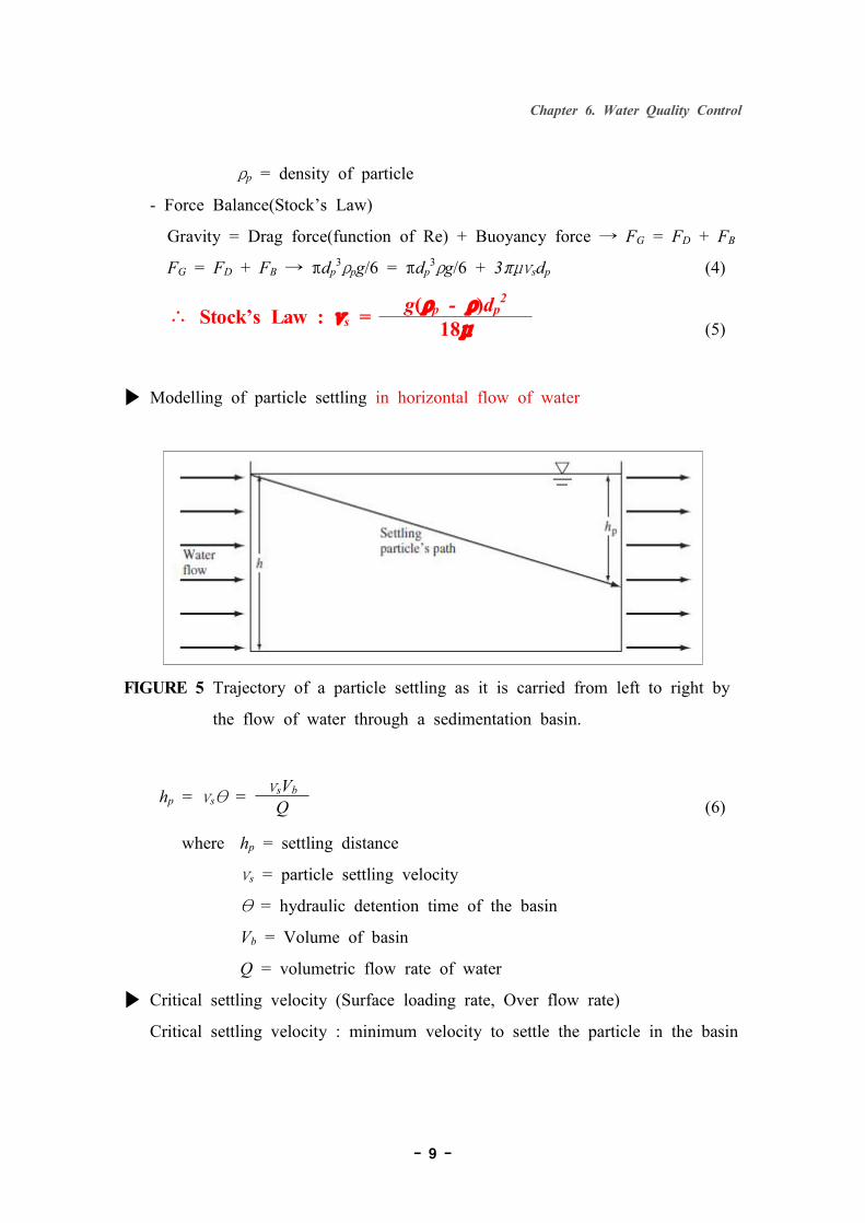
▶ Modelling of particle settling in horizontal flow of water
FIGURE 5 Trajectory of a particle settling as it is carried from left to right by
the flow of water through a sedimentation basin.
hp = νsθ = νsVb
Q (6)
where hp = settling distance
νs = particle settling velocity
θ = hydraulic detention time of the basin
Vb = Volume of basin
Q = volumetric flow rate of water
▶ Critical settling velocity (Surface loading rate, Over flow rate)
Critical settling velocity : minimum velocity to settle the particle in the basin
Page 10
Chapter 6. Water Quality Control
- 10 -
Critical settling velocity(νo) = h = hQ = hQ = Qθ Vb hAb Ab (7)
where Ab = Surface area of rectangular basin
So, minimum surface area of the basin to settle the particle must be
Minimum surface area(Ab) =
18Qμ
g(ρp - ρ)dp2 (8)
▶ Typical Design Parameter for Settler for WTP
- Settling velocity, Surface loading rate, Over flow rate = 1.0 ∼ 2.5 m/hr
- Detention time, Hydraulic Retention Time(HRT) = 1.0 ∼ 4.0 hr
EXAMPLE 1 Silt Removal in a Clarifier
A drinking water treatment plant uses a circular sedimentation basin to treat
3.0 MGD of river water. (MGD = million gallons/day = 0.0438 m3/s, a common
U.S. measure of flow rate used for water and wastewater treatment.). After
storms occur upstream, the river often carries 0.010 mm silt particles with an
average density of 2.2 g/cm3, and the silt must be removed before the water can
be used. The plant’s clarifier is 3.5 m deep and 21 m in diameter. The water is
15℃.
<Given Data>
Q = 3.0 MGD = 0.1314 m3/s = 473 m3/hr
dp = 0.01 mm = 0.01×10⁻³ m = 1×10⁻⁵ m
ρp = 2.2 g/cm3, = 2,200 kg/m3
hb = 3.5 m
ODb = 21 m
Temperature = 15℃
→ ρw = 999.1 kg/m3, μw = 0.00114 kg/(m∙s) = 4.104 kg/(m∙hr)
<Question>
1. θ = ?
Page 11
Chapter 6. Water Quality Control
- 11 -
2. Will the clarifier remove all of the silt particles from the river water?
<Solution>
1. θ = Vb = hb × (π ODb2/4) = 3.5 m π×212 m2
= 2.56 hrQ Q 473 m3/hr 4
2. From EQ(8), minimum surface area(Ab) is
Ab=18Qμ
=18×0.1314m3 0.00114kg s2 m3
g(ρp - ρ)dp2 s m∙s 9.8m (2200–999.1)kg 1×10⁻¹⁰m2
= 2,291 m2
Real surface area = πODb2 / 4= π × 212 / 4 =346.4 m2
So, this settler was too small to remove all of the silt particles from the river
water.
Page 12
Chapter 6. Water Quality Control
- 12 -
5.2 Coagulation and Flocculation
▶ Colloid : particles in the size range of about 0.01 ∼ 1㎛▶ Characteristics of most colloids in water treatment
- net negative surface charge
- causes the particles to repel each other
- tend to be suspended in solution
▶ Principle of coagulation : alter the particle surfaces to adhere to each other
▶ Goal of coagulation : size up to remove particles by settlement or filtration
▶ Purpose of coagulant
- neutralize the surface charge
- allowing the particles to come together to form larger particles
- more easily removed through sedimentation, filtration and etc.
▶ Usual coagulant
- alum(Al2(SO4)3∙18H2O)
- PACL(Poly-Aluminum-Chloride, AlCl3)
- Poly electrolytes like FeCl3, FeSO4 and etc
▶ Mechanism of coagulation
- alum ionizes in water(producing ions)
- some ions neutralize the negative charges on the colloids
- most of the aluminum ions react with alkalinity(bicarbonate) in the water
- form insoluble aluminum hydroxide, Al(OH)3. : light and fluffy floc
Al2(SO4)3∙18H2O + 6HCO3– ⇌ 2Al(OH)3↓ + 6CO2 + 18H2O + 3SO4
2– (10)
Alum Aluminum Sulfate
hydroxide
- for sufficient bicarbonate, adding lime(Ca(OH)2), Sodium carbonate(Na2CO3)
Page 13
Chapter 6. Water Quality Control
- 13 -
- Al(OH)3 adsorbs on the surface of colloidal(colloid + SS)
→ aggregation of particles → grow by colliding with each other → settle
▶ Collision efficiency factor(α)
- Expression of the degree of particle destabilization
- Collision efficiency factor(α) = number of aggregated colloidsnumber of collisions of colloids
∙α = 1.0 : every collision results in aggregation
∙α = 0.25 : 25% of collisions results in aggregation
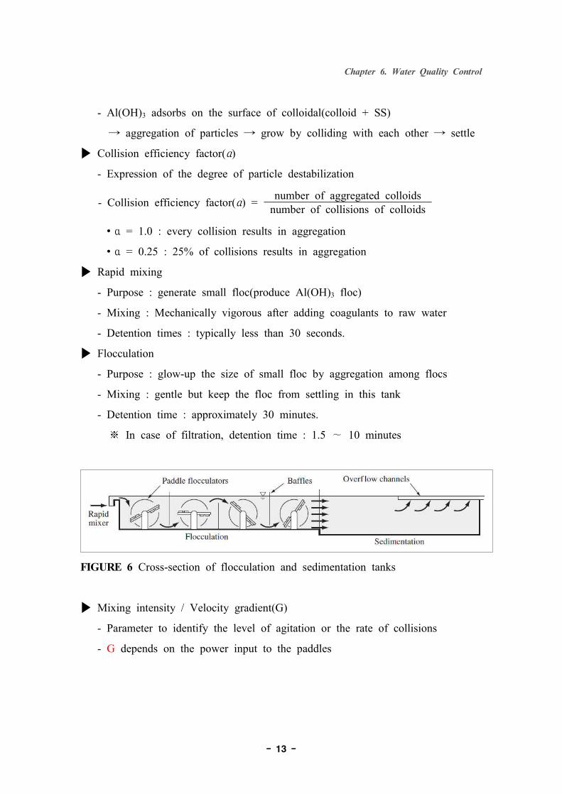
▶ Rapid mixing
- Purpose : generate small floc(produce Al(OH)3 floc)
- Mixing : Mechanically vigorous after adding coagulants to raw water
- Detention times : typically less than 30 seconds.
▶ Flocculation
- Purpose : glow-up the size of small floc by aggregation among flocs
- Mixing : gentle but keep the floc from settling in this tank
- Detention time : approximately 30 minutes.
※ In case of filtration, detention time : 1.5 ∼ 10 minutes
FIGURE 6 Cross-section of flocculation and sedimentation tanks
▶ Mixing intensity / Velocity gradient(G)
- Parameter to identify the level of agitation or the rate of collisions
- G depends on the power input to the paddles
Page 14
Chapter 6. Water Quality Control
- 14 -
(11)
where P = power input to the paddles (or other mixing method)
Vb = volume of the vessel
μ = viscosity of the water
▶ Concentration of particle(N)
- Number of aggregated particles↑ → Total number of particles↓
- Concentration of particle(N) = Total number of particlesVolume of water
▶ Modelling of the 1st order flocculation rate(dN/dt)
<Assumption>
① Mono-disperse distribution : all the particles are initially the same size
② Laminar mixing : water mixing is relatively mild
③ Coalescing aggregation : aggregate’s volume is the sum of the volumes of
the individual particles comprising the aggregate
▶ The 1st flocculation rate(dN/dt) = r(N) = - kN (12)
where k = α4ΩGπ (13)
α = collision efficiency factor
Ω = floc volume concentration(solids volume concentration)
= πdp3N0 = constant by assuming coalescing aggregation (14)6
dp = diameter of particle
N0 = initial number concentration of mono-disperse particles
EXAMPLE 2 Silt Flocculation Before Sedimentation
To improve their settling, the 0.010 mm silt particles in Example 1 are
completely destabilized by adding alum and are passed through one of two
side-by-side, well-mixed flocculation chambers. The chambers are cubic with each
Page 15
Chapter 6. Water Quality Control
- 15 -
dimension being 3.5 m. They are mixed with paddle mixers that input 2.50 kW
of power into the water in each chamber. The water entering the flocculation
chamber contains 105 particles per mL. What is the average diameter of the
aggregates leaving the flocculation chambers?
<Given Data>
Total Q = 3.0 MGD = 0.01314 m3/s
(2 Chamber → Q/chamber = 0.00657 m3/s)
dp = 0.01 mm = 0.01×10⁻³ m = 1×10⁻⁵ m
P = 2.5 kW = 2,500 W
Vb = 3.5 m × 3.5 m × 3.5 m = 42.875 m3
μ = viscosity of the water = 0.001145 kg/(m∙s)
N0 = 105 ea/ml
<Question> da leaving the flocculation chamber ?
<Solution>
FIGURE 7 Schematic of single flocculation basin with variables defined.
From Eq(11),
= = 226 s–1
Mass Balance at stead-state : QN0 = QN + VbkN
Page 16
Chapter 6. Water Quality Control
- 16 -
By using Eq(13), k = α4ΩGπ
From mass balance, QN0 = QN + α4ΩGVbNπ
QN0 = Q + α4ΩGVb →N0 = 1 + α4ΩGVb
N π N πQ
Ω = πdp3N0 = π(1×10⁻⁵ m3) 105 ea 106 mL = 5.24 × 10⁻⁵ 6 6 ea mL m3
Let’s assume, α = 1.0 for silt, then
N0 = 1 + α4ΩGVb = 1 + 4(5.24 × 10⁻⁵)(226 s–1)(42.875 m3) = 10.8N πQ π(0.0657 m3/s)
By assumption 3, Vd = Va → N0(dp)3 = N(da)3
∴ da = ( N0 )1/3 dp = (10.8)1/3 × 0.01 mm = 0.0221 mmN
Page 17
Chapter 6. Water Quality Control
- 17 -
5.3 Filtration
▶ Purpose of filtration : removal of small particles including pathogens
▶ Rapid depth filtration : the most common filtration technique in WTP
- Sand Filter(SF)
- Dual Media Filter(DMF) or Multi-Media Filter(MMF)
- Fiber Filter
▶ Structure : layer or layers of carefully sieved filter media
▶ Filter media
- Classical depth filter : sand, anthracite coal, diatomaceous earth, on top of
a bed of graded gravels.
- Advanced depth filter : PP fiber
▶ Filtration pore : openings between the media grains
▶ Pore size : bigger than size of the particles
▶ Important removal mechanism
- Simple sieving between media
- adsorption
- continued flocculation, and sedimentation in the pore spaces
▶ Operating cycle
Filtration → Backwash → Rinse → Filtration
※ When the filter becomes clogged with particles, the filter is shut down
for a short period of time and cleaned by forcing water backwards
through the media.
▶ Filtration velocity(va) : loading rates or superficial velocities
- Definition : input flow rate(Q) / filter’s cross sectional area(Af)
- Range of Filtration velocity(va) : 2∼8 gpm/ft2(5∼20 m/hr)
Page 18
Chapter 6. Water Quality Control
- 18 -
va = QAf (15)
Filter Efficiency(Production Efficiency) (ηa) = Vf – Vb – Vr
Vf (16)
Effective filtration rate(ref) = Vf/Af–Vb/Af–Vr/Af = (Vf–Vb–Vr)tf + tb + tr Af tc (17)
where Vf = filtrate volume / filter cycle(m3)
Vb = backwash water volume / filter cycle(m3)
Vr = rinse water volume after backwash / filter cycle(m3)
tf = filtration duration time(hr)
tb = backwashing duration time(hr)
tr = rinsing duration time(hr)
tc = operating cycle time to complete filter cycle(hr)
▶ ηa for rapid depth filters : > 95%
5.4 Disinfection
▶ Objectives of disinfection
- kill any pathogens in the water(primary disinfection)
- secondary(or residual) disinfection
▶ Disinfectant based on the free chlorine
- chlorine gas(Cl2)
- sodium hypochlorite(NaOCl)
- calcium hypochlorite(Ca(OCl)2).
Cl2(aq) + H2O = HOCl + H+ + Cl– (18)
HOCl = OCl– + H+
▶ Strength as disinfectant : Hypochlorous acid(HOCl) > hypochlorite(OCl–)
Page 19
Chapter 6. Water Quality Control
- 19 -
→ free chlorine disinfection is usually conducted in slightly acidic water
▶ Free chlorine
- very effective as secondary disinfection of the filtrate
- very effective against bacteria
- less effective with protozoan cysts of Giardia lamblia and Cryptosporidium
- less effective with viruses
▶ Chloramines (NH2Cl, NHCl2, and NCl3)
- Combined chlorine by adding ammonia to the filtrate
- Increase the lifetime of this residual
- Less effective as oxidants than HOCl(not used as primary disinfectants)
▶ Disadvantage of free chlorine
- Formation of the halogenated disinfectant byproducts(carcinogen)
∙DBPs include trihalomethanes (THMs)
∙Chloroform(CHCl3)
∙Haloacetic acids (HAAs)
▶ Approach to reducing THMs
- Remove more of the organics before chlorination
※ Pre-chlorination(chlorination of incoming raw water before processing)
∙Common practice in the past to kill algae
∙Big contribution to the formation of DBPs
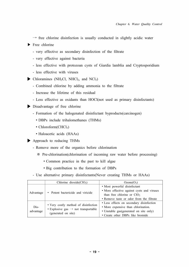
- Use alternative primary disinfectants(Never creating THMs or HAAs)
Chlorine dioxide(ClO2) Ozone(O3)
Advantage ∙ Potent bactericide and viricide
∙Most powerful disinfectant∙More effective against cysts and viruses than free chlorine or ClO2
∙Remove taste or odor from the filtrate
Dis-advantage
∙Very costly method of disinfection∙Explosive gas → not transportable (generated on site)
∙Less effects on secondary disinfection∙More expensive than chlorination.∙Unstable gas(generated on site only)∙Create other DBPs like bromide
Page 20
Chapter 6. Water Quality Control
- 20 -
▶ Modelling of the rate of inactivation of pathogens during disinfection
(Chick-Watson model)
r(N) = dN/dt = - kCnN (19)
where r(N) = rate of the change in the pathogen concentration
N = number of pathogens/unit volume
C = concentration of disinfectant
n = coefficient of dilution(empirical constant)
k = coefficient of specific lethality(empirical rate constant)
※ n = 1 for many cases
k = f (pathogen, disinfectant, temperature, and pH)
To simplify Eq(19), use a first-order reduction of pathogen concentration by
assuming Cn is constant and lumping k and Cn into a single rate constant, k*, as
r(N) = dN/dt = - k*N (20)
EXAMPLE 3 Giardia Inactivation by Ozone
Because of the purity of its groundwater source, a water utility only has to
disinfect the water before delivery. The utility uses ozone as its primary
disinfectant and treats 10 MGD (million gallons per day) of water. The ozone is
bubbled into the water as it passes sequentially through the four chambers of a
disinfectant contact tank (see Figure 8). Each chamber of the tank is well mixed,
holds 50,000 gallons of water, and receives the same ozone dose. As discussed
earlier in Section 3, EPA requires that the Giardia concentration be reduced to
11,000 of its initial concentration(referred to as 3-log reduction). What is the
minimum ozone concentration that must be used to achieve the required removal
of Giardia? The coefficient of specific lethality and coefficient of dilution for
ozone inactivation of Giardia under these conditions are 1.8 L∙mg-1∙min-1 and
1.0, respectively.
Page 21
Chapter 6. Water Quality Control
- 21 -
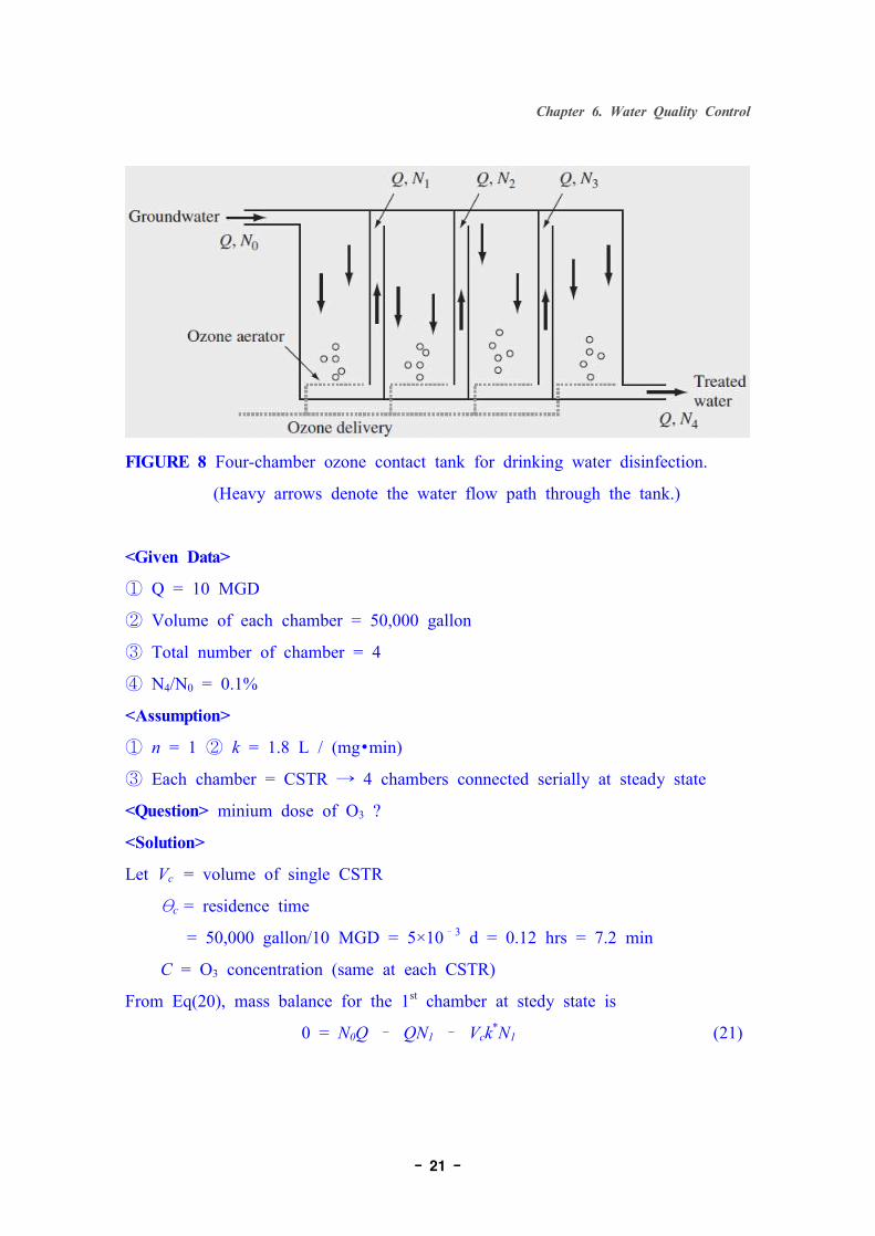
FIGURE 8 Four-chamber ozone contact tank for drinking water disinfection.
(Heavy arrows denote the water flow path through the tank.)
<Given Data>
① Q = 10 MGD
② Volume of each chamber = 50,000 gallon
③ Total number of chamber = 4
④ N4/N0 = 0.1%
<Assumption>
① n = 1 ② k = 1.8 L / (mg∙min)
③ Each chamber = CSTR → 4 chambers connected serially at steady state
<Question> minium dose of O3 ?
<Solution>
Let Vc = volume of single CSTR
θc = residence time
= 50,000 gallon/10 MGD = 5×10⁻³ d = 0.12 hrs = 7.2 min
C = O3 concentration (same at each CSTR)
From Eq(20), mass balance for the 1st chamber at stedy state is
0 = N0Q – QN1 – Vck*N1 (21)
Page 22
Chapter 6. Water Quality Control
- 22 -
N1 = Q N0 →N1 = Q
Q–Vck* N0 Q–Vck*
Since θc = Vc / Q, N1 = Q = 1N0 Q–Vck* 1 – θck* (22)
Similary, mass balance for the 2nd chamber is
N2 = Q = 1N1 Q–Vck* 1 – θck* (23)
Then N2 = N2 × N1 = 1N0 N1 N0 (1 – θck*)2 (24)
For m chamber of CSTR, Nm = 1N0 (1 – θck*)m (25)
For 4 chamber of CSTR, N4 = 1N0 (1 – θck*)4 and n=1, k* = kCn = kC
N4 =1,000 = 1 = 1 = 1 = 1N0 (1–θck*)4 (1–θckC)4 (1–7.2×1.8 C)4 (1–12.96 C)4
∴ C = 0.36 mg/L
5.5 Hardness and Alkalinity
▶ Hardness
- Defined as the concentration of all multivalent metallic cations
(Ca, Mg, Fe, Sr, Al and etc)
- Typical hardness : sum of only Ca+2 and Mg+2.
- Groundwater is especially prone to excessive hardness
- Hardness causes two distinct problems. First, the reaction between hardness
▶ Disadvantage of hardness
- Produces a sticky, gummy deposit called “soap curd” with soap
- Generate scaling problem(CaCO3 and Mg(OH)2 by heating)
▶ Equivalents and Equivalent weights.
Page 23
Chapter 6. Water Quality Control
- 23 -
Equivalent weight(EW) = Atomic or Molecular Wightn (27)
where n = ionic charge
For example,
EW of CaCO3 = (40+12+3×16) = 100 = 50 g/eq = 50 mg/meq2 2 (28)
EW of Ca2+ = 40.1≈ 20.0 mg/meq2
Equivalent concentration ofmultivalent cations of X(meq/L) = Concentration of X(mg/L)
EW of X(mg/meq) (29)
mg/L of X as CaCO3 = Conc. of X(mg/L) × 50.0 mg CaCO3/meqEW of X(mg/meq) (30)
TABLE 3 Equivalent weights for selected ions, and compounds
EXAMPLE 4 Expressing the Concentration of Hardness
Page 24
Chapter 6. Water Quality Control
- 24 -
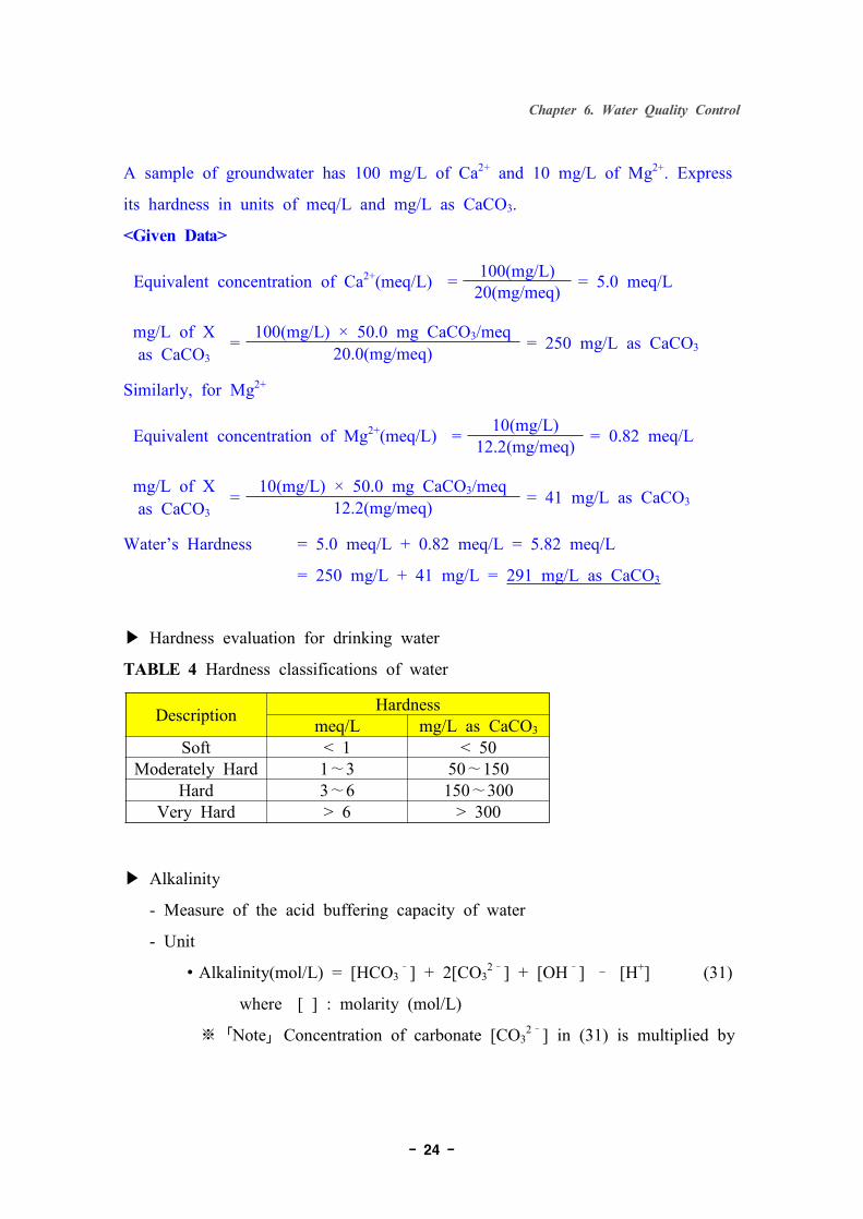
A sample of groundwater has 100 mg/L of Ca2+ and 10 mg/L of Mg2+. Express
its hardness in units of meq/L and mg/L as CaCO3.
<Given Data>
Equivalent concentration of Ca2+(meq/L) = 100(mg/L) = 5.0 meq/L20(mg/meq)
mg/L of Xas CaCO3
= 100(mg/L) × 50.0 mg CaCO3/meq = 250 mg/L as CaCO320.0(mg/meq)
Similarly, for Mg2+
Equivalent concentration of Mg2+(meq/L) = 10(mg/L) = 0.82 meq/L12.2(mg/meq)
mg/L of Xas CaCO3
= 10(mg/L) × 50.0 mg CaCO3/meq = 41 mg/L as CaCO312.2(mg/meq)
Water’s Hardness = 5.0 meq/L + 0.82 meq/L = 5.82 meq/L
= 250 mg/L + 41 mg/L = 291 mg/L as CaCO3
▶ Hardness evaluation for drinking water
TABLE 4 Hardness classifications of water
Description Hardnessmeq/L mg/L as CaCO3
Soft < 1 < 50Moderately Hard 1∼3 50∼150
Hard 3∼6 150∼300Very Hard > 6 > 300
▶ Alkalinity
- Measure of the acid buffering capacity of water
- Unit
∙Alkalinity(mol/L) = [HCO3–] + 2[CO3
2–] + [OH–] – [H+] (31)
where [ ] : molarity (mol/L)
※「Note」Concentration of carbonate [CO32–] in (31) is multiplied by
Page 25
Chapter 6. Water Quality Control
- 25 -
2, because each carbonate ion can neutralize two H+ ions.
∙ Alkalinity(meq/L) = (HCO3–) + (CO3
2–) + (OH–) – (H+) (32)
where ( ) : concentration in meg/L or mg/L of CaCO3
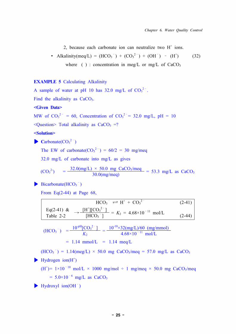
EXAMPLE 5 Calculating Alkalinity
A sample of water at pH 10 has 32.0 mg/L of CO32–.
Find the alkalinity as CaCO3.
<Given Data>
MW of CO32– = 60, Concentration of CO3
2–= 32.0 mg/L, pH = 10
<Question> Total alkalinity as CaCO3 =?
<Solution>
▶ Carbonate(CO32–)
The EW of carbonate(CO32–) = 60/2 = 30 mg/meq
32.0 mg/L of carbonate into mg/L as gives
(CO32-) = 32.0(mg/L) × 50.0 mg CaCO3/meq = 53.3 mg/L as CaCO330.0(mg/meq)
▶ Bicarbonate(HCO3–)
From Eq(2-44) at Page 68,
HCO3– ⇄ H+ + CO3
2– (2-41)Eq(2-41) &Table 2-2 →
[H+][CO32–] = K2 = 4.68×10⁻¹¹ mol/L[HCO3–] (2-44)
(HCO3–) = 10-pH[CO3
2–] = 10-10×32(mg/L)/60 (mg/mmol)K2 4.68×10⁻¹¹ mol/L
= 1.14 mmol/L = 1.14 meq/L
(HCO3–) = 1.14(meg/L) × 50.0 mg CaCO3/meq = 57.0 mg/L as CaCO3
▶ Hydrogen ion(H+)
(H+)= 1×10⁻¹⁰ mol/L × 1000 mg/mol ÷ 1 mg/meq × 50.0 mg CaCO3/meq
= 5.0×10⁻⁶ mg/L as CaCO3
▶ Hydroxyl ion(OH–)
Page 26
Chapter 6. Water Quality Control
- 26 -
[H+][OH–] = 10–14 and [H] = 10–10 → [OH–] = 10–4 mol/L
(OH–)=1×10⁻⁴ mol/L × 17,000 mg/mol ÷ 17 mg/meq × 50.0 mg CaCO3/meq
= 5.0 mg/L as CaCO3
▶ From Eq(32), total alkalinity is
(HCO3–)+(CO3
2–)+(OH–)–(H+)=53.3+57.0+5.0-5.0×10–6=115.3mg/L as CaCO3
▶ For nearly neutral water (pH between 6 and 8.5)
- Molarity of CO32–, OH–, H+ : very small
- Alkalinity(meq/L) = [HCO3–] for 6 ≤ pH ≤ 8.5 (34)
▶ Total hardness(TH) by assuming only Ca+2 + Mg+2 in water
- TH = Sum of individual hardness components = Ca+2 + Mg+2 (35)
- TH = Carbonate hardness(CH) + noncarbonate hardness(NCH)
∙ CH associated with the anions(HCO3–, CO3
2–
※ temporary hardness(can be removed by heating)
∙ NCH associated with other anions
- Alkalinity([HCO3–]+[CO3
2–]) ≥ TH → CH = TH and NCH = 0
- Alkalinity([HCO3–]+[CO3
2–]) ≤ TH → CH=alkalinity and NCH=TH–CH
▶ Scaling : Ca+2 + 2HCO3– ↔ CaCO3 + CO2 + H2O (36)
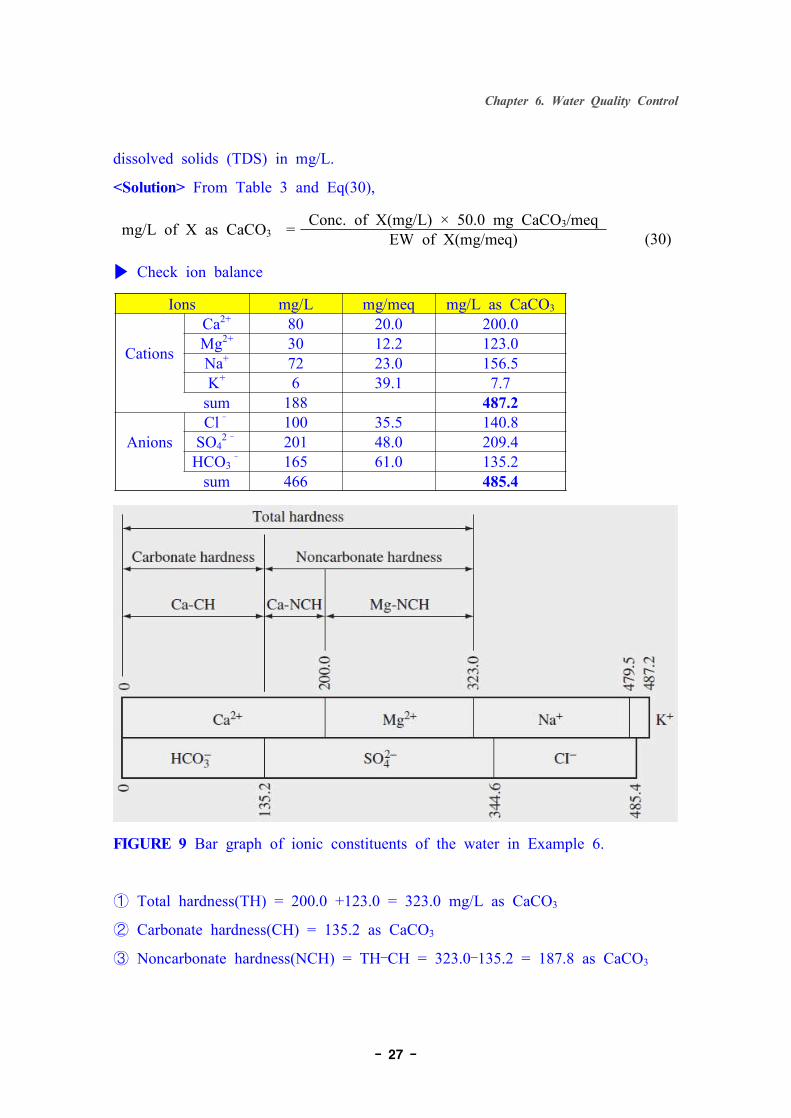
EXAMPLE 6 Chemical Analysis of a Sample of Water
The analysis of a sample of water with pH 7.5 has produced the following
concentrations(mg/L):
Cations AnionsCa2+ 80 Cl– 100Mg2+ 30 SO4
2– 201Na+ 72 HCO3
– 165K+ 6
Find the total hardness (TH), the carbonate hardness (CH), the noncarbonate
hardness (NCH), and the alkalinity, all expressed as CaCO3. Find the total
Page 27
Chapter 6. Water Quality Control
- 27 -
dissolved solids (TDS) in mg/L.
<Solution> From Table 3 and Eq(30),
mg/L of X as CaCO3 = Conc. of X(mg/L) × 50.0 mg CaCO3/meqEW of X(mg/meq) (30)
▶ Check ion balance
Ions mg/L mg/meq mg/L as CaCO3
Cations
Ca2+ 80 20.0 200.0Mg2+ 30 12.2 123.0Na+ 72 23.0 156.5K+ 6 39.1 7.7
sum 188 487.2
AnionsCl– 100 35.5 140.8
SO42– 201 48.0 209.4
HCO3– 165 61.0 135.2
sum 466 485.4
FIGURE 9 Bar graph of ionic constituents of the water in Example 6.
➀ Total hardness(TH) = 200.0 +123.0 = 323.0 mg/L as CaCO3
➁ Carbonate hardness(CH) = 135.2 as CaCO3
➂ Noncarbonate hardness(NCH) = TH–CH = 323.0–135.2 = 187.8 as CaCO3
Page 28
Chapter 6. Water Quality Control
- 28 -
➃ pH≈neutral → (H+) and (OH–)≈0 → Alkalinity≈(HCO3–) =135.2 mg/L
➄ Total dissolved solids(TDS) = 188 mg/L + 466 mg/L = 654 mg/L
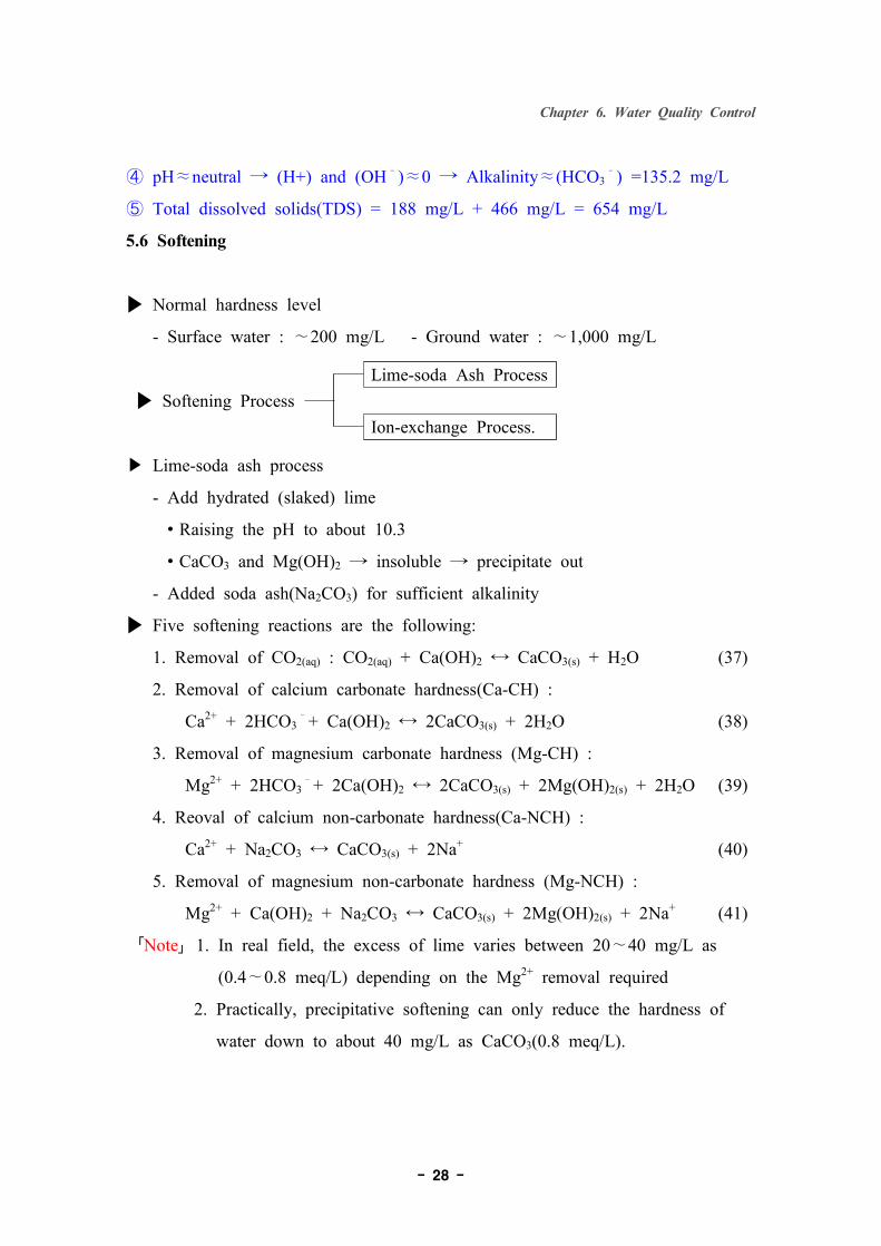
5.6 Softening
▶ Normal hardness level
- Surface water : ∼200 mg/L - Ground water : ∼1,000 mg/L
Lime-soda Ash Process▶ Softening Process
Ion-exchange Process.
▶ Lime-soda ash process
- Add hydrated (slaked) lime
∙Raising the pH to about 10.3
∙CaCO3 and Mg(OH)2 → insoluble → precipitate out
- Added soda ash(Na2CO3) for sufficient alkalinity
▶ Five softening reactions are the following:
1. Removal of CO2(aq) : CO2(aq) + Ca(OH)2 ↔ CaCO3(s) + H2O (37)
2. Removal of calcium carbonate hardness(Ca-CH) :
Ca2+ + 2HCO3–+ Ca(OH)2 ↔ 2CaCO3(s) + 2H2O (38)
3. Removal of magnesium carbonate hardness (Mg-CH) :
Mg2+ + 2HCO3–+ 2Ca(OH)2 ↔ 2CaCO3(s) + 2Mg(OH)2(s) + 2H2O (39)
4. Reoval of calcium non-carbonate hardness(Ca-NCH) :
Ca2+ + Na2CO3 ↔ CaCO3(s) + 2Na+ (40)
5. Removal of magnesium non-carbonate hardness (Mg-NCH) :
Mg2+ + Ca(OH)2 + Na2CO3 ↔ CaCO3(s) + 2Mg(OH)2(s) + 2Na+ (41)
「Note」1. In real field, the excess of lime varies between 20∼40 mg/L as
(0.4∼0.8 meq/L) depending on the Mg2+ removal required
2. Practically, precipitative softening can only reduce the hardness of
water down to about 40 mg/L as CaCO3(0.8 meq/L).
Page 29
Chapter 6. Water Quality Control
- 29 -
EXAMPLE 7 Lime-Soda Ash Softening
A utility treats 12 MGD of the water in Example 6.
1. Lime and soda ash(in mg/L as CaCO3) ?, 2. Softening sludge daily ?
<Given Data> pH = 7.5, Q = 12 MGD
Ions mg/L mg/meq mg/L as CaCO3
Cations
Ca2+ 80 20.0 200.0Mg2+ 30 12.2 123.0Na+ 72 23.0 156.5K+ 6 39.1 7.7
sum 188 487.2
AnionsCl– 100 35.5 140.8
SO42– 201 48.0 209.4
HCO3– 165 61.0 135.2
sum 466 485.4
<Solution>
1. Calculate the amount of CO2(aq) that must be neutralized.
From <Example 6>, pH = 7.5, and [HCO3–] = 165 mg/L = 0.002705 M
[CO2(aq)] = [HCO3–][H+] = (2.7105×10⁻³ M)(10–7.5 M) = 1.914×10⁻⁴ MK1 (4.47×10⁻⁷ M)
So, CO2(aq) as CaCO3 = 1.914×10–4 M × 100(MW of CaCO3) = 19.14
2. Draw a bar graph for the system
TABLE 5 Components, lime and soda ash dosage, and solids generated in
softening the water in Example 6
Component Concentration(mg/L CaCO3)
Lime(mg/L CaCO3)
Soda Ash(mg/L CaCO3)
CaCO3(s)
(mg/L CaCO3)Mg(OH)2(s)
(mg/L CaCO3)CO2(aq) 19.1 19.1 0 19.1 0Ca-CH 135.2 135.2 0 270.4 0Mg-CH 0 0 0 0 0Ca-NCH 64.8 0 64.8 64.8 0Mg-NCH 123.0 123.0 123.0 123.0 123.0
Exess 20Total 297.3 187.8 477.3 123.0
Page 30
Chapter 6. Water Quality Control
- 30 -
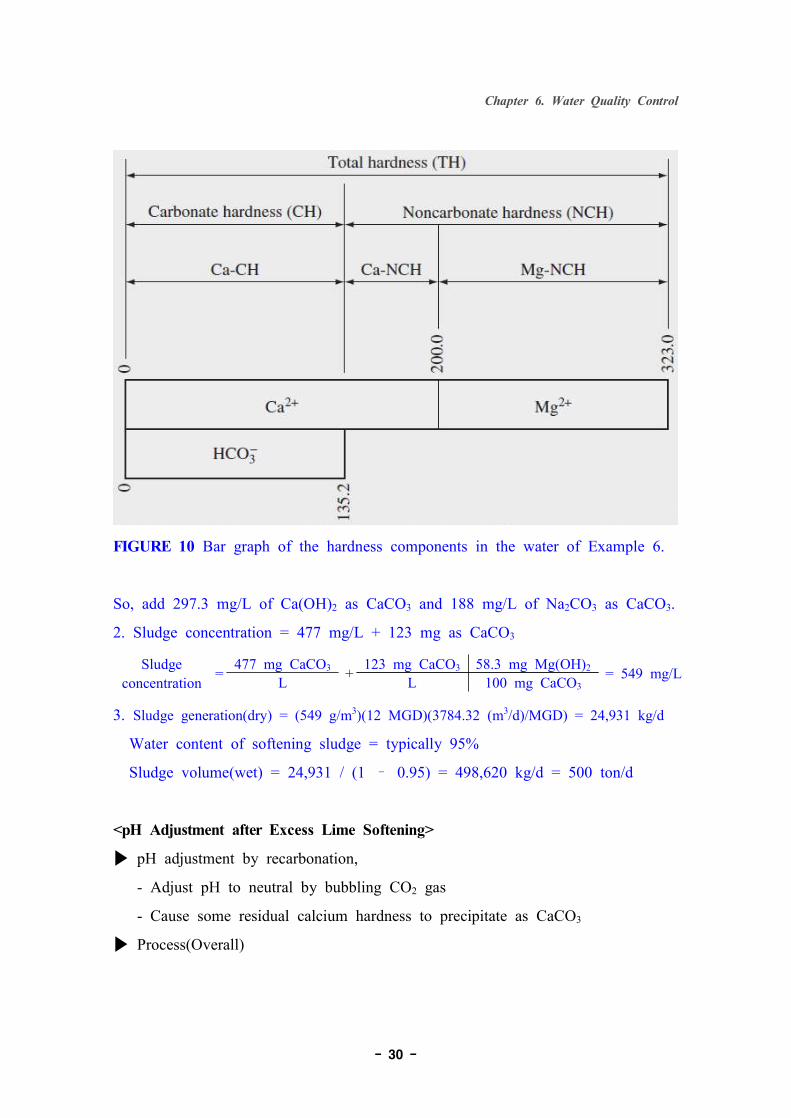
FIGURE 10 Bar graph of the hardness components in the water of Example 6.
So, add 297.3 mg/L of Ca(OH)2 as CaCO3 and 188 mg/L of Na2CO3 as CaCO3.
2. Sludge concentration = 477 mg/L + 123 mg as CaCO3
Sludgeconcentration = 477 mg CaCO3 + 123 mg CaCO3 58.3 mg Mg(OH)2 = 549 mg/LL L 100 mg CaCO3
3. Sludge generation(dry) = (549 g/m3)(12 MGD)(3784.32 (m3/d)/MGD) = 24,931 kg/d
Water content of softening sludge = typically 95%
Sludge volume(wet) = 24,931 / (1 – 0.95) = 498,620 kg/d = 500 ton/d
<pH Adjustment after Excess Lime Softening>
▶ pH adjustment by recarbonation,
- Adjust pH to neutral by bubbling CO2 gas
- Cause some residual calcium hardness to precipitate as CaCO3
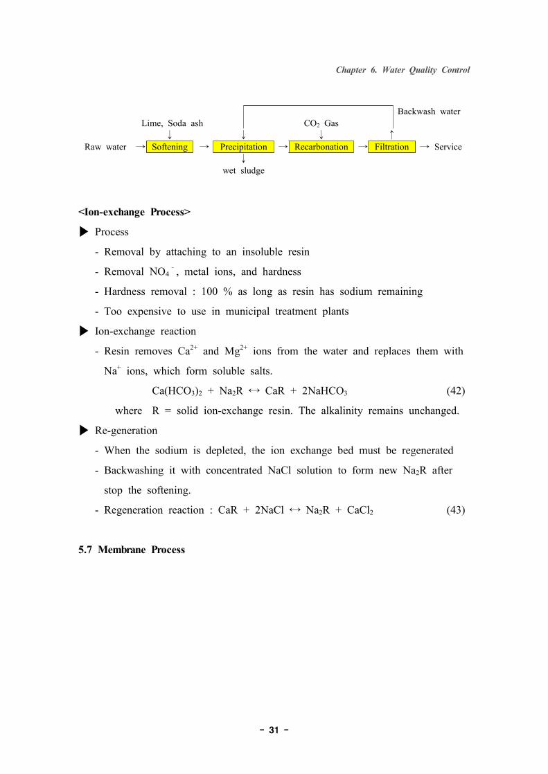
▶ Process(Overall)
Page 31
Chapter 6. Water Quality Control
- 31 -
Backwash waterLime, Soda ash CO2 Gas
↓ ↓ ↓ ↑
Raw water → Softening → Precipitation → Recarbonation → Filtration → Service↓
wet sludge
<Ion-exchange Process>
▶ Process
- Removal by attaching to an insoluble resin
- Removal NO4–, metal ions, and hardness
- Hardness removal : 100 % as long as resin has sodium remaining
- Too expensive to use in municipal treatment plants
▶ Ion-exchange reaction
- Resin removes Ca2+ and Mg2+ ions from the water and replaces them with
Na+ ions, which form soluble salts.
Ca(HCO3)2 + Na2R ↔ CaR + 2NaHCO3 (42)
where R = solid ion-exchange resin. The alkalinity remains unchanged.
▶ Re-generation
- When the sodium is depleted, the ion exchange bed must be regenerated
- Backwashing it with concentrated NaCl solution to form new Na2R after
stop the softening.
- Regeneration reaction : CaR + 2NaCl ↔ Na2R + CaCl2 (43)
5.7 Membrane Process
Page 32
Chapter 6. Water Quality Control
- 32 -
FIGURE 11 Size ranges and types of contaminants removed by membrane
processes.(Source: Adapted from Taylor and Wiesner, 1999.)
▶ Rejection(R) = 1 – Cp (45), Recovery(r) = Qp (46)CF QF
▶ Range of R and r :
- For MF/UF : R > 99% for most case and r > typically 90%
- For NF/BWRO : R > 97% and 75% < r < 90%
- For SWRO : R > 99% and 40% < r < 55% for SWRO
Page 33
Chapter 6. Water Quality Control
- 33 -
5. Wastewater Treatment
TABLE 6 Composition of Untreated Domestic Wastewater
Total Dissolved Solid(TDS) : dissolved solid, colloidal solid, very small SS
▶ Total Solid (TS)
Suspended Solid(SS) : Filterable particle(> 1.4 ㎛)
▶ Basic Process : Raw → Primary → Secondary → Tertiary → Discharge
Purpose : Remove big matters
Remove soluble one
- Remove SS- Emergency
Facilities : - Screen- Settler
- Bio-treat- Settler
- Filtration- Flotation
BOD removal : 35% 90% - 50% without chemical- 70% with chemical
SS removal : 60% 90%- 60% without chemical- 90% with chemical
Nutrients removal : - T-N < 50%- T-P < 33% for conventional process
Page 34
Chapter 6. Water Quality Control
- 34 -
FIGURE 12 Schematic of a typical wastewater treatment facility providing
primary and secondary treatment.
5.1 Primary Treatment
▶ Purpose : Preliminary remove big matters to prevent from damaging the
pumps or clog small pipes.
▶ Typical screening size : 2 ∼ 7 cm
▶ Grit chamber
- Settle out sand, grit, and other heavy material
- Detention time : typically 20 to 30 s
▶ Primary settling tank
- Settle out most of SS by gravity
- Detention time : 1.5 ∼ 3.0 hours
- Removal efficiency : 50 ∼ 65% of SS, 25 ∼ 40% of the BOD
※ Primary sludge or raw sludge : solids removed at primary treatment tank
▶ High-rate clarifiers
- Enhanced settling speed of SS
∙by adding various coagulants and ballast(additives such as sand that
make the settling particles more dense)
Page 35
Chapter 6. Water Quality Control
- 35 -
∙specialized settling equipment within the clarifier,
- Range of overflow rates or surface loading rate(vo) : 1,000 ∼ 3,000 m/d
※ vo of conventional clarification : 30 ∼ 100 m/d
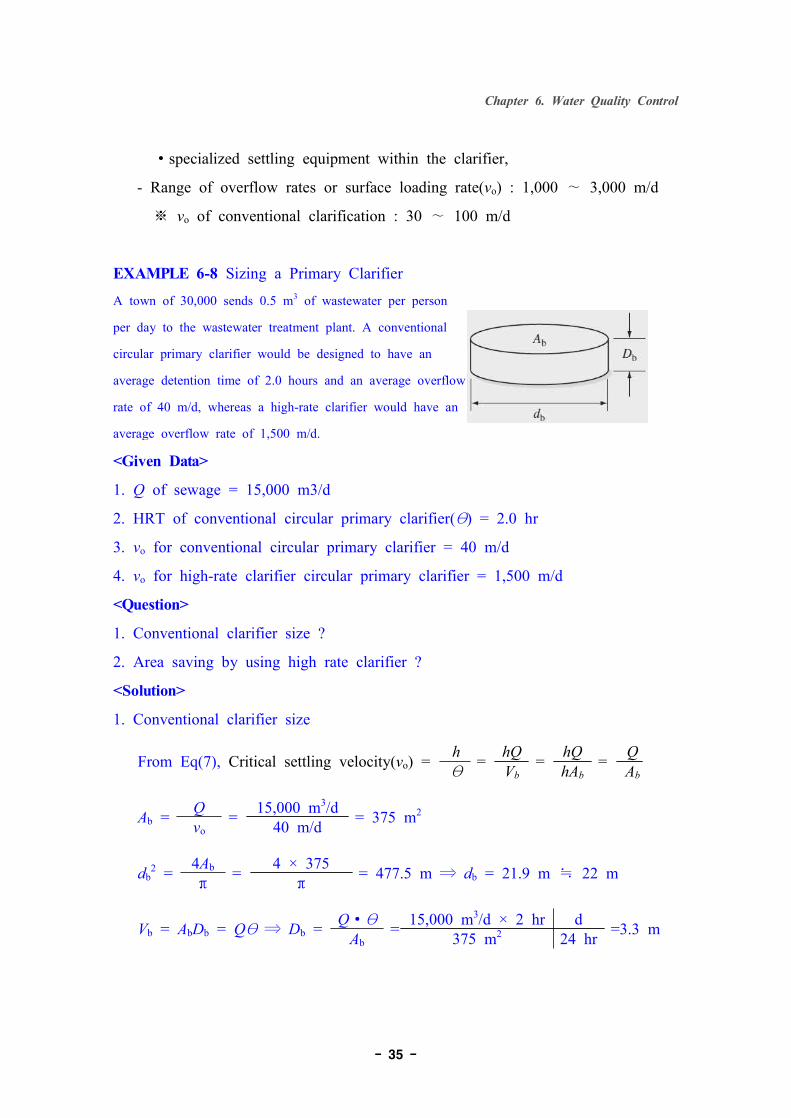
EXAMPLE 6-8 Sizing a Primary Clarifier
A town of 30,000 sends 0.5 m3 of wastewater per person
per day to the wastewater treatment plant. A conventional
circular primary clarifier would be designed to have an
average detention time of 2.0 hours and an average overflow
rate of 40 m/d, whereas a high-rate clarifier would have an
average overflow rate of 1,500 m/d.
<Given Data>
1. Q of sewage = 15,000 m3/d
2. HRT of conventional circular primary clarifier(θ) = 2.0 hr
3. vo for conventional circular primary clarifier = 40 m/d
4. vo for high-rate clarifier circular primary clarifier = 1,500 m/d
<Question>
1. Conventional clarifier size ?
2. Area saving by using high rate clarifier ?
<Solution>
1. Conventional clarifier size
From Eq(7), Critical settling velocity(vo) = h = hQ = hQ = Qθ Vb hAb Ab
Ab = Q = 15,000 m3/d = 375 m2
vo 40 m/d
db2 = 4Ab = 4 × 375 = 477.5 m ⇒ db = 21.9 m ≒ 22 m
π π
Vb = AbDb = Qθ ⇒ Db = Q∙θ = 15,000 m3/d × 2 hr d =3.3 mAb 375 m2 24 hr
Page 36
Chapter 6. Water Quality Control
- 36 -
So, dimension according to conventional design : 22m(ID)×3.3(H)
2. Area saving by using high rate clarifier ?
Ab = Q = 15,000 m3/d = 10 m2
vo 1,500 m/d
So, 97% of the land would be saved by changing the clarifier to high rate
clarifier, if other auxiliary equipments like coagulation tank was not
considered.
5.2 Secondary (Biological) Treatment
▶ Main purpose : Removal of BOD and SS
▶ Treatment process
- Suspended growth : microorganisms are suspended in and move with the
water.
- Attached growth : microorganisms are fixed on a stationary surface, and
the water flows past the microorganisms
5.3 Microbial Kinetics
▶ Substrate : organic matter that microorganisms consume(as mg/L of BOD)
▶ VSS(Volatile Suspended Solids, mg/L) or VS(Volatile Solids).
after drying at 105°C(Concentration = SS) ←
Difference in mass of solids→ after burning off at 500°C
(VSS or VS)
<Cell Birth Rate>
- Mass balances for water, substrate, and microbe mass
▶ The 1st order growth rate
Microbial mass growth rate(rg) = dX = μXdt (47)
where X = concentration of microorganism, VSS/L
μ = specific bio mass growth rate constant(time–1)
Page 37
Chapter 6. Water Quality Control
- 37 -
(dependent on the availability of substrate)
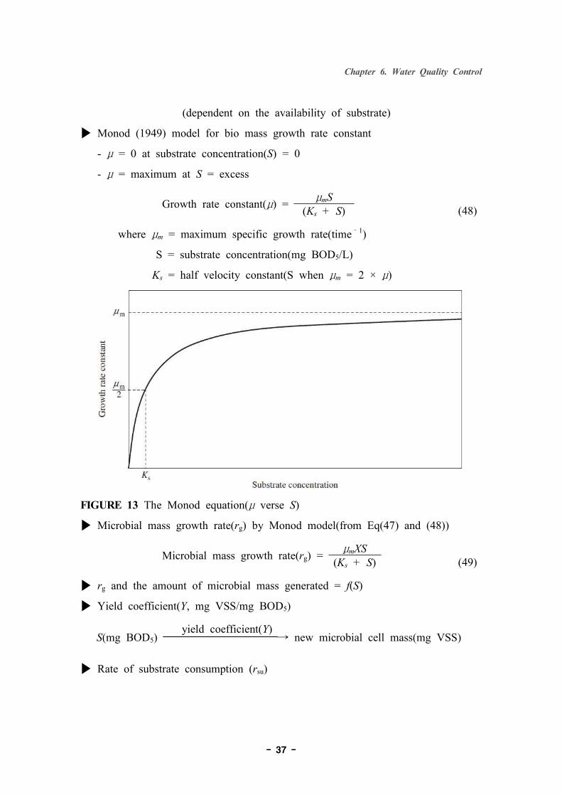
▶ Monod (1949) model for bio mass growth rate constant
- μ = 0 at substrate concentration(S) = 0
- μ = maximum at S = excess
Growth rate constant(μ) = μmS(Ks + S) (48)
where μm = maximum specific growth rate(time–1)
S = substrate concentration(mg BOD5/L)
Ks = half velocity constant(S when μm = 2 × μ)
FIGURE 13 The Monod equation(μ verse S)
▶ Microbial mass growth rate(rg) by Monod model(from Eq(47) and (48))
Microbial mass growth rate(rg) = μmXS(Ks + S) (49)
▶ rg and the amount of microbial mass generated = f(S)
▶ Yield coefficient(Y, mg VSS/mg BOD5)
S(mg BOD5)
yield coefficient(Y)→ new microbial cell mass(mg VSS)
▶ Rate of substrate consumption (rsu)
Page 38
Chapter 6. Water Quality Control
- 38 -
Rate of substrate consumption(rsu) = dS = –rg = - μmXSdt Y Y(Ks + S) (50)
▶ Maximum specific substrate utilization constant(k)
Maximum specific substrate utilization constant(k) = μm
Y (51)
From Eq(49), (50) and (51),
Rate of substrate consumption(rsu)=dS = –rg = - μmXS = - kXSdt Y Y(Ks+S) (Ks+S) (52)
<Cell Death Rate>
▶ Death rate for microbes(rd) = the 1st order with a negative reaction term
Death rate for microbes(rd) = dX =–kdXdt (53)
where kd = endogenous decay(death) rate constant(time–1)
<Kinetic Analysis of a Bioreactor>
▶ Net or observed rate of change of microbe concentration(r´g)
Net rate of change of microbe concentration(r´g) = rg + rd = μmXS–kdX(Ks+S) (54)
※ Reaction rate is the difference between the rate of birth(49) and rate of
death(53).
From Eq(50) and (54), (r´g) = rg + rd = –Yrsu –kdX (55)
※ Reaction rate for microbial growth is proportional to the rate that substrate
is consumed(rsu) minus the rate microbes die(rd).
TABLE 7 Typical Microbial Kinetic Parameters (All are given for 20°C)
Page 39
Chapter 6. Water Quality Control
- 39 -
EXAMPLE 6-9 BOD Consumption in Pond
The shallow pond depicted in Figure 14 stays well mixed due to the wind and
the steady flow through of a small creek.
FIGURE 14 A pond in which microbial activity consumes organic matter.
If the microbes in the pond consume the inflowing biodegradable organic matter
according to typical kinetics, determine :
1. The BOD5 leaving the pond
2. The biodegradable organic matter removal efficiency of the pond
3. The concentration of volatile suspended solids leaving the pond
<Assumptions>
1. Pond : CSTR in steady state
2. Flow rate and composition : at a steady for a long period
<Question>
1. Sf = ?
Page 40
Chapter 6. Water Quality Control
- 40 -
2. (So – Sf) / So = ?
3. Xf = ?
<Solution>
1. Mass balance on the microbial mass
0 = QXo–QXf + Vr´g = 0–QX + Vr´g = Vr´g–QX ⇒ 0 = θr´g–X (56)
Eq(56) → Eq(54) : 0 = θμmXS–θkdX–X ⇒ 1 = θμmS
–θkd(Ks+S) (Ks+S)
∴ S = Ks(1 + θkd)(θμm–1–θkd) (57)
- θ = 200 m3/(50 m3/day) = 4.0 day,
- From Table 7, default values for kinetic parameter are
Ks = 60 mg BOD5/L, kd = 0.06 day–1, μm = 3 day–1
S = Ks(1 + θkd) = 60 mg BOD5 (1+4×0.06) = 6.9 mg BOD5/L(θμm–1–θkd) L (4×3–1–4×0.06)
2. Efficiency =(So–Sf) × 100 =
(95–6.9) mg BOD5/L × 100 = 92.7 %So 95 mg BOD5/L
3. Substrate mass balance at steady state
0 = QSo–QSf + Vrsu = QSo–QS + Vrsu (59)
Eq(52) → Eq(59) : 0 = QSo–QS– VkXS⇒ Q(So–S) = VkXS
(Ks+S) (Ks+S)
- From Table 7, k = 5 mg BOD5/(mg VSS∙day)
∴ X= Q(So–S)(Ks+S) = (So–S)(Ks+S) = (95–6.9)(60+6.9) =42.7 mg VSS/LVkS θkS 4×5×6.9
『Note』BOD5 in the outflowing creek is underestimated substantially
▶ much of the microbial mass generated could actually be used as substrate by
other predatory microbes → cause a significant oxygen demand
▶ removal efficiency calculated is based only on the decrease in the original
quantity of biodegradable organic matter entering the pond and doesn’t
account for the organic matter synthesized in the pond.
Page 41
Chapter 6. Water Quality Control
- 41 -
5.4 Suspended Growth Treatment
AS(Activated Sludge)
Suspended Growth Treatment Aerated Lagoons
MBR(Membrane Bio-Reactor)
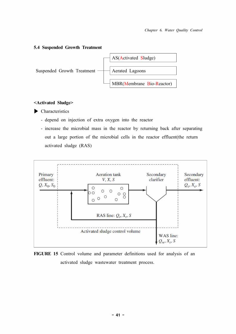
<Activated Sludge>
▶ Characteristics
- depend on injection of extra oxygen into the reactor
- increase the microbial mass in the reactor by returning back after separating
out a large portion of the microbial cells in the reactor effluent(the return
activated sludge (RAS)
FIGURE 15 Control volume and parameter definitions used for analysis of an
activated sludge wastewater treatment process.
Page 42
Chapter 6. Water Quality Control
- 42 -
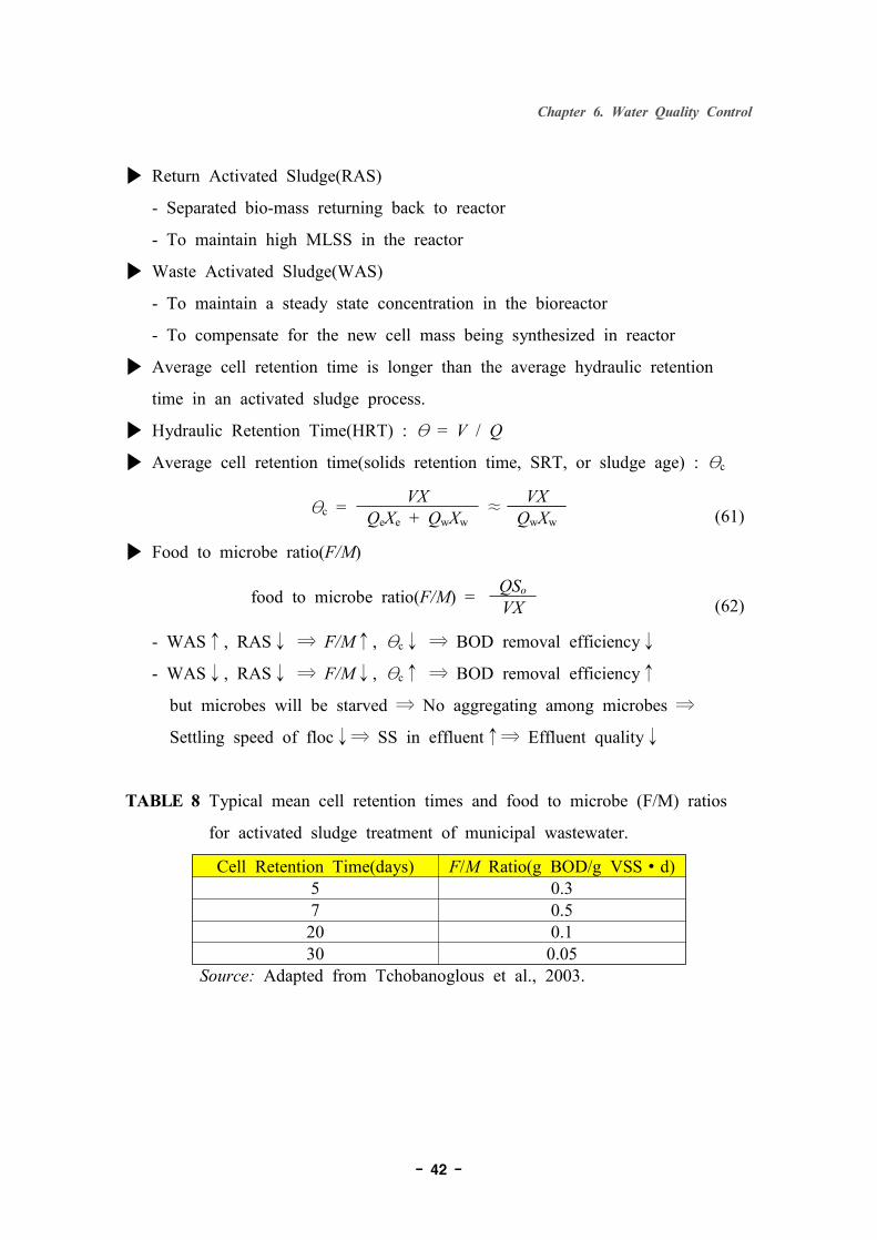
▶ Return Activated Sludge(RAS)
- Separated bio-mass returning back to reactor
- To maintain high MLSS in the reactor
▶ Waste Activated Sludge(WAS)
- To maintain a steady state concentration in the bioreactor
- To compensate for the new cell mass being synthesized in reactor
▶ Average cell retention time is longer than the average hydraulic retention
time in an activated sludge process.
▶ Hydraulic Retention Time(HRT) : θ = V / Q
▶ Average cell retention time(solids retention time, SRT, or sludge age) : θc
θc = VX≈
VXQeXe + QwXw QwXw (61)
▶ Food to microbe ratio(F/M)
food to microbe ratio(F/M) = QSo
VX (62)
- WAS↑, RAS↓ ⇒ F/M↑, θc↓ ⇒ BOD removal efficiency↓
- WAS↓, RAS↓ ⇒ F/M↓, θc↑ ⇒ BOD removal efficiency↑
but microbes will be starved ⇒ No aggregating among microbes ⇒
Settling speed of floc↓⇒ SS in effluent↑⇒ Effluent quality↓
TABLE 8 Typical mean cell retention times and food to microbe (F/M) ratios
for activated sludge treatment of municipal wastewater.
Cell Retention Time(days) F/M Ratio(g BOD/g VSS∙d)5 0.37 0.5
20 0.130 0.05
Source: Adapted from Tchobanoglous et al., 2003.
Page 43
Chapter 6. Water Quality Control
- 43 -
FIGURE 16 Approximate concentrations of BOD5, SS, T-N, and T-P at
conventional STP (Source: Based on Hammer and Hammer, 1996.)
<Membrane Bio-Reactors(MBR)>
▶ Purpose of MBR
- delete secondary clarifier
- improve the suspended solids separation efficiency
▶ Structure and Operation Principle ⇒ Refer to PPT file prepared separately
<Aerated Lagoons and Oxidation Ponds>
Page 44
Chapter 6. Water Quality Control
- 44 -
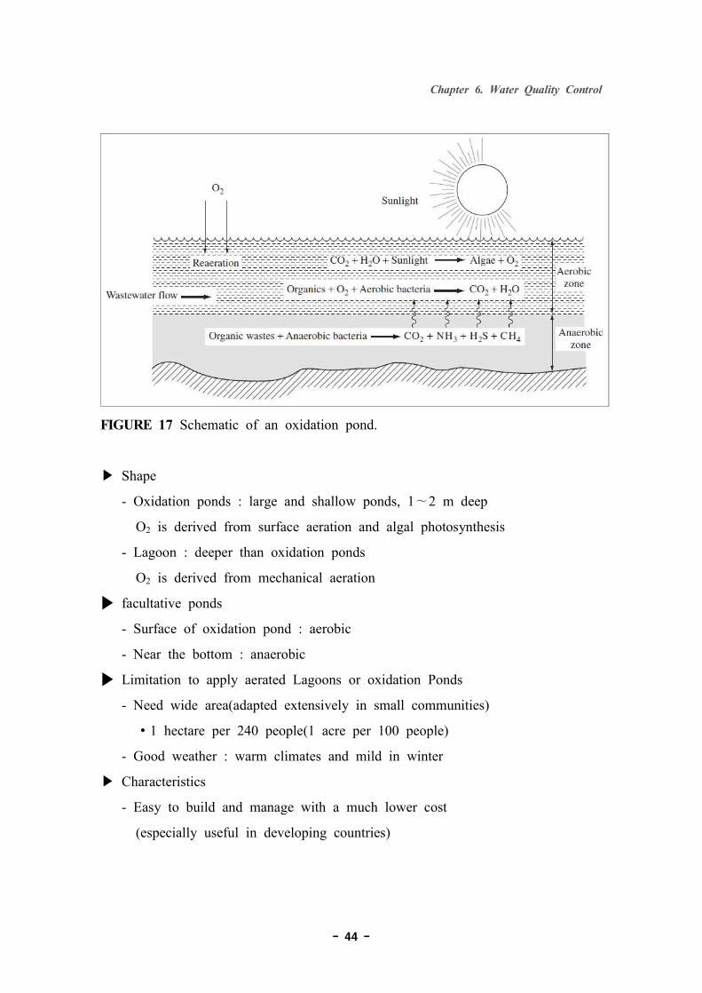
FIGURE 17 Schematic of an oxidation pond.
▶ Shape
- Oxidation ponds : large and shallow ponds, 1∼2 m deep
O2 is derived from surface aeration and algal photosynthesis
- Lagoon : deeper than oxidation ponds
O2 is derived from mechanical aeration
▶ facultative ponds
- Surface of oxidation pond : aerobic
- Near the bottom : anaerobic
▶ Limitation to apply aerated Lagoons or oxidation Ponds
- Need wide area(adapted extensively in small communities)
∙1 hectare per 240 people(1 acre per 100 people)
- Good weather : warm climates and mild in winter
▶ Characteristics
- Easy to build and manage with a much lower cost
(especially useful in developing countries)
Page 45
Chapter 6. Water Quality Control
- 45 -
- Accommodate large fluctuations in flow
- Produce unpleasant odors.
- Effluent quality may not meet the regulation(30 mg/L of BOD5 and SS)
Page 46
Chapter 6. Water Quality Control
- 46 -
5.5 Attached Growth Treatment
secondary treatment process
Attached Growth Treatment
Pre-treatment of activated sludge process
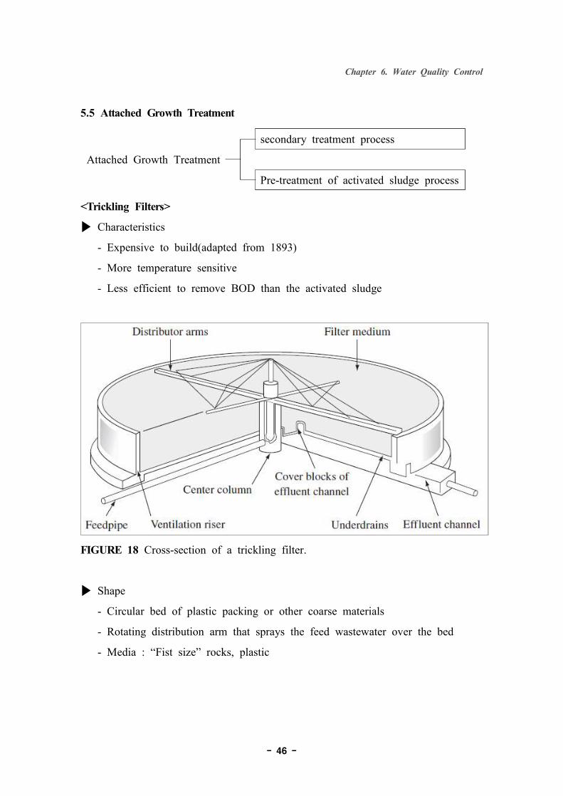
<Trickling Filters>
▶ Characteristics
- Expensive to build(adapted from 1893)
- More temperature sensitive
- Less efficient to remove BOD than the activated sludge
FIGURE 18 Cross-section of a trickling filter.
▶ Shape
- Circular bed of plastic packing or other coarse materials
- Rotating distribution arm that sprays the feed wastewater over the bed
- Media : “Fist size” rocks, plastic
Page 47
Chapter 6. Water Quality Control
- 47 -
<Rotating Biological Contactor(RBC)>
FIGURE 19 RBC cross-section and treatment system: (a) RBC cross-section; (b)
RBC series included in a secondary wastewater treatment system.
▶ Shape
- Series of closely spaced, circular, plastic disks, typically 3.6 m in diameter
- Attached to a rotating horizontal shaft
- Bottom 40% of each disk is submersed in a tank
- Biomass film that grows on the surface of the disks
▶ Characteristics
- More efficient than trickling filters to remove pollutants
- Easier to operate under varying load conditions than trickling filters
(because it is easier to keep the solid medium wet at all times)
Page 48
Chapter 6. Water Quality Control
- 48 -
5.6 Hybrid Suspended/Attached Growth Systems
▶ Developed and employed since the mid-1980s
▶ Decrease the cost and time to remove organic matter
▶ Fixed or suspended media submerged in the activated sludge tank
- More innovative and recent hybrid systems
- Microbial biofilms grow on the media surface
- Improve effluent clarification
- Maintain high MLSS(low F/M ratios)
▶ moving-bed biofilm reactors, fluidized bed biological reactors, submerged
fixed-film activated sludge reactors, and submerged rotating biological reactors
in Tchobanoglous et al. (2003).
Page 49
Chapter 6. Water Quality Control
- 49 -
5.7 Sludge Treatment
▶ Amount of sludge production : about 2% of WW(volume)
(Water content of sludge : about 97%)
▶ Cost of disposal based on volume of sludge
▶ Primary goals of sludge treatment
- lower the water content as possible
- Stabilize the solids
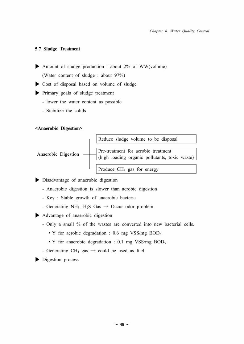
<Anaerobic Digestion>
Reduce sludge volume to be disposal
Anaerobic Digestion Pre-treatment for aerobic treatment(high loading organic pollutants, toxic waste)
Produce CH4 gas for energy
▶ Disadvantage of anaerobic digestion
- Anaerobic digestion is slower than aerobic digestion
- Key : Stable growth of anaerobic bacteria
- Generating NH3, H2S Gas → Occur odor problem
▶ Advantage of anaerobic digestion
- Only a small % of the wastes are converted into new bacterial cells.
∙Y for aerobic degradation : 0.6 mg VSS/mg BOD5
∙Y for anaerobic degradation : 0.1 mg VSS/mg BOD5
- Generating CH4 gas → could be used as fuel
▶ Digestion process
Page 50
Chapter 6. Water Quality Control
- 50 -
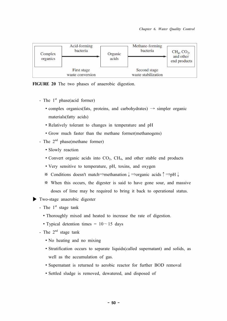
FIGURE 20 The two phases of anaerobic digestion.
- The 1st phase(acid former)
∙complex organics(fats, proteins, and carbohydrates) → simpler organic
materials(fatty acids)
∙Relatively tolerant to changes in temperature and pH
∙Grow much faster than the methane former(methanogens)
- The 2nd phase(methane former)
∙Slowly reaction
∙Convert organic acids into CO2, CH4, and other stable end products
∙Very sensitive to temperature, pH, toxins, and oxygen
※ Conditions doesn't match⇒methanation↓⇒organic acids↑⇒pH↓
※ When this occurs, the digester is said to have gone sour, and massive
doses of lime may be required to bring it back to operational status.
▶ Two-stage anaerobic digester
- The 1st stage tank
∙Thoroughly mixed and heated to increase the rate of digestion.
∙Typical detention times = 10∼15 days
- The 2nd stage tank
∙No heating and no mixing
∙Stratification occurs to separate liquids(called supernatant) and solids, as
well as the accumulation of gas.
∙Supernatant is returned to aerobic reactor for further BOD removal
∙Settled sludge is removed, dewatered, and disposed of
Page 51
Chapter 6. Water Quality Control
- 51 -
∙Gas produced in the digester is about 60% CH4
FIGURE 21 Schematic of a two-stage anaerobic digester.
Page 52
Chapter 6. Water Quality Control
- 52 -
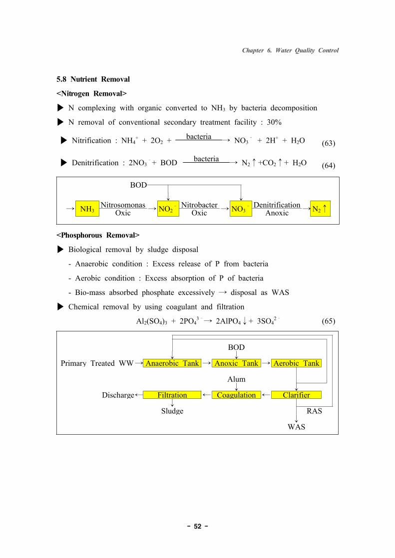
5.8 Nutrient Removal
<Nitrogen Removal>
▶ N complexing with organic converted to NH3 by bacteria decomposition
▶ N removal of conventional secondary treatment facility : 30%
▶ Nitrification : NH4+ + 2O2 + bacteria
→ NO3– + 2H+ + H2O (63)
▶ Denitrification : 2NO3–+ BOD bacteria → N2↑+CO2↑+ H2O (64)
BOD↓ ↓
→ NH3Nitrosomonas
→ NO2– Nitrobacter
→ NO3– Denitrification
→N2↑Oxic Oxic Anoxic
<Phosphorous Removal>
▶ Biological removal by sludge disposal
- Anaerobic condition : Excess release of P from bacteria
- Aerobic condition : Excess absorption of P of bacteria
- Bio-mass absorbed phosphate excessively → disposal as WAS
▶ Chemical removal by using coagulant and filtration
Al2(SO4)3 + 2PO43–→ 2AlPO4↓+ 3SO4
2– (65)
BOD↓ ↓
Primary Treated WW→ Anaerobic Tank → Anoxic Tank → Aerobic Tank
Alum↓ ↓
Discharge← Filtration ← Coagulation ← Clarifier↓
Sludge RAS↓
WAS