110

CHAPTER 6

OPTIMAL SIZING AND LOCATION OF DISTRIBUTED

GENERATORS USING MODIFIED BACTERIAL

FORAGING ALGORITHM UNDER VARIABLE

LOADING CONDITIONS

6.1 INTRODUCTION

Around the world, conventional power systems are facing the

problems of gradual depletion of fossil fuel resources, poor energy efficiency

and environmental pollution. Many private sectors invest huge money to meet

their contingent loads under power cut and also cater peak load demand

locally using conventional diesel generators. These problems have led to a

new trend of power locally at the distribution voltage level using non-

conventional/ renewable energy sources like Natural gas, Biogas, Wind-

power, Solar Energy and Fuel cells, Combined Heat and Power (CHP)

systems, Micro turbines, and Sterling Engines and their integration into the

utility distribution networks. This type of power generation is termed as

distributed generation and the energy sources are termed as distributed energy

distinguish this concept of generation from centralized conventional

generation. The distribution network becomes active with the integration of

D.G. and hence is termed as active distribution network Durga & Nadarajah

(2007).

114

can again be connected to the utility as a separate semi-

autonomous entity.

Stand-a

generation augmentation, thereby improving overall power

quality and reliability. Moreover, a deregulated environment

and open access to the distribution network also provide greater

opportunities for D.G. integration. In some countries, the fuel

diversity offered by DG is considered valuable, while in some

developing countries, the shortage of power is so acute that any

form of generation is encouraged to meet the load demand.

6.4 TYPES OF DG DEVICE

The D.G. device utilized in this paper is I.C Engine. The internal

combustion engine is an engine in which the combustion of a fuel (normally a

fossil fuel) occurs with an oxidizer (usually air) in a combustion chamber. In

an internal combustion engine, the expansion of the high-temperature and

high -pressure gases produced by combustion apply direct force to some

component of the engine. This force is applied typically to pistons, turbine

blades, or a nozzle. This force moves the component over a distance,

transforming chemical energy into useful mechanical energy. The first

functioning internal combustion engine was created by Étienne Lenoir.

ICEs cost less than its peers such as fuel cells and are of the

conventional form of energy. They can be integrated directly into the power

grid as compared to renewable forms like wind, solar that need power

converters for linkage purposes. Table 6.1 list out the various types of DG

device, their operation range and their utility interface.

115

Table 6.1 Various types of DG devices, their operation range andmeans

of implementation

Technology Typical Capability Ranges Utility Interface

Solar Cells A few W to several hundred kW

dc to ac converter

Wind A few hundred W to a few MW

Asynchronous generator

Geothermal A few hundred kW to a few MW

Synchronous generator

Ocean A few hundred kW to a few MW

Four-quadrant synchronous machine

Internal combustion engine

A few hundred kW to tens of MW

Synchronous generator or ac to ac converter

Combined cycle A few tens of MW to hundreds of MW

Synchronous generator

Combustion turbine

A few MW to hundreds of MW

Synchronous generator.

Micro turbines A few tens of kW to a few MW

ac to ac converter

Fuel cells A few tens of kW to a few tens of MW

dc to ac converter

6.5 MODIFIED BACTERIAL FORAGING ALGORITHM FOR

OPF

The following section explains the various steps involved in

implementation of Bacterial Foraging Algorithm (BFA) for the above

formulated problem. BFA is based on the principle of foraging theory and

used to solve numerous engineering problems. The advantages of BFA such

116

as speedy convergence, self-adaptive, computationally intensive etc. make it

superior over other existing intelligent techniques. The basic Bacterial

Foraging Optimization consists of three principal mechanisms; namely

chemotaxis, reproduction and elimination-dispersal. In case of MBFA the

chemotaxis step of normal BFA is altered by introducing variable step size in

each iteration (Hanning et al 2009).

Step 1: Initialization

1) S - Number of bacteria

2) p - Dimension of the search space.

3) sN - Swimming length, the maximum number of steps each

bacteria swims before tumbling

4) cN - Number of iterations to be undertaken in a chemotactic

loop;

5) reN - Maximum number of reproduction to be undertaken;

6) reN - Maximum number of elimination and dispersal;

7) edP - Probability of elimination and dispersal ;

8) )(iC - Unit run length for bacterium

9) Sii ........,,3,2,1, - Random Swim direction

Step 2: Read bus data, line data, active power limits and cost coefficients of

generator including DG

Step 3: Run Newton-Raphson (NR) load flow.

The following section explains the chemotaxis loop, swarming,

reproduction, and elimination and dispersion of a bacterium. Any

117

thi bacteria at the thj chemotactic, thk reproduction and thl

elimination stage is given by ),,( lkji and its corresponding

objective function is ),,,( lkjiJ . The values of ),,( lkji and

),,,( lkjiJ are updated using the following steps.

Step 4: Start Elimination dispersal loop 1ll

Step 5: Reproduction loop 1kk

Step 6: Chemotaxis loop 1jj

A) For each bacterium Si .......,,3,2,1 , compute objective function

),,,( lkjiJ .

a. Let )),,(),,,((),,,(),,,( lkjPlkjJlkjiJlkjiJ iccsw

b. Let ),,,( lkjiJJ swlast , to save this value since we find a

better cost via a run.

c. End of the loop

B) Tumble: Generate a random vector Pi)( with each element

being a random number in the range of [0,1]

C) Move:

Let )(i = )()(

)(ii

iT

)()(),,(),,1( iiClkjlkj ii

This results in a step size )(iC in the direction of the tumble for

the i th bacterium.

118

D) Compute ),,1,( lkjiJ and then let

)),,1(),,,1((),,1,(),,1,( lkjPlkjJlkjiJlkjiJ iccsw

E) Swim

a. Let m = 0 (counter length for swim)

b. While SNm

i. Let 1mm

ii. If lastsw JlkjiJ ),,1,(

then ),,1,( lkjiJJ swlast

)()(),,(),,1( iiClkjlkj ii

and use the above ),,1( lkji to compute

new ),,1,( lkjiJ

iii. Else SNm

F) Go to next bacterium )1(i till all the bacteria undergo

chemotaxis.

G) Update the run length unit using Equation (6.1)

Step 7: Reproduction

a. For the given k and l , for each Si ....,..........,3,2,1 , let 1

1),,,(

cNj

jsw

ihealth lkjiJJ be the health of i th bacterium and sort

healthJ in ascending order

119

b. The bacteria with the highest healthJ values die and those with

minimum values split and the already made copies are now

placed at the same location as their parent.

Step 8: If reNk , go to step 4. In this case, we have not reached the

number of specified reproduction steps, so we start the next

generation in the chemotactic loop.

Step 9: Elimination dispersal: for Si ....,..........,3,2,1 , a random number is

generated and if it is less than or equal to edP , then that bacterium

is dispersed to a new random location else it remains at its original

location. If edNl , then go to step 4; otherwise go to next step

Step 10: Run Newton-Raphson load flow

Step 11: Print OPF Results and end.

The flowchart for the proposed method is shown in Figure 6.1. The

flowchart for finding the optimal location and size of the DG using MBFA

algorithm is shown in Figure 6.2. The parameters selected for the proposed

MBFA algorithm are as follows.

Number of bacteria S : 20

Number of chemotactic steps Nc : 5

Swimming length Ns : 4

of reproduction steps Nre : 4

Number of elimination and dispersal events Ned : 2

Probability of elimination and dispersal Ped : 0.2

120

Depth of attractant : 0.01

Width of attractant : 0.04

Height of repellent : 0.01

Width of repellent : 10.0

6.6 PSEUDO CODE FOR OPTIMAL LOCATION AND SIZE OF

DG USING MBFA

Step 1: DG size and Maximum DG limit should be initialized.

Step 2: Objective Function should be evaluated using MBFA and Optimal

DG location should be updated.

Step 3: The DG size should be increased in all Load buses

Step 4: The condition , is to be checked, if yes go to step 5, else

go back to step 2.

Step 5: The DG size in optimal location is to be increased.

Step 6: Objective Function should be evaluated using MBFA and Optimal

DG location should be updated.

Step 7: The condition , is to be checked, if yes goto step 8 else

goto step 5

Step 8: Optimal DG location and size to be printed.

Step 9: Terminate

121

Figure 6.1 Flowchart for OPF using BFA

Initialize: BFA parameters Read power system

Run NR Load Flow

Compute OF for bacterium

Compute new OF

Tumble bacterium for a step size of along a randomly generated tumble vector

Set

Run NR Load Flow

Print OPF Results

=

End

Start

Elimination-Dispersal

Reproduction

X

X

Y

Y

Yes

No

Yes

Yes

Yes

Yes

Yes

No

No

No

No

No

122

Figure 6.2 Flowchart for obtaining optimal location and size of DG

using MBFA

Start

Initialize DG size ,

Evaluate Objective function using MBFA and update optimal DG Location

Increase DG Size in all Load buses

Increase DG Size in Optimal Location

Evaluate Objective function using MBFA and update optimal DG Size

Print: Optimal DG location and Size

End

No

No

Yes

Yes

123

6.7 RESULTS AND DISCUSSIONS

To solve the effectiveness of the proposed MBFA algorithm, in

finding the optimal location and rating of DG in IEEE 14 and IEEE 30 bus

system are used. A Matlab program is written and executed in intel core i5

3.2GHz processor system. The Distributed Generation data available in the

literature Durga & Nadarajah (2007) is used in this work. The quadratic cost

coefficients of DG used are given in Table 6.2. The line data, bus data and

generator data of IEEE 30 and IEEE 14 bus test systems are presented in

Appendix 1 and 2 respectively.

Table 6.2 Distributed Generation data

d ($/MW2h) e ($/MWh) f ($/h)

0.002 15 0

6.7.1 Variation of Objective Function (OF) with DG Placement

The problem formulated in chapter 3 is solved using proposed

BFOA algorithm. In this work, IC engine is considered as Distributed

Generator and it is added to the load buses of IEEE14 and IEEE30 bus

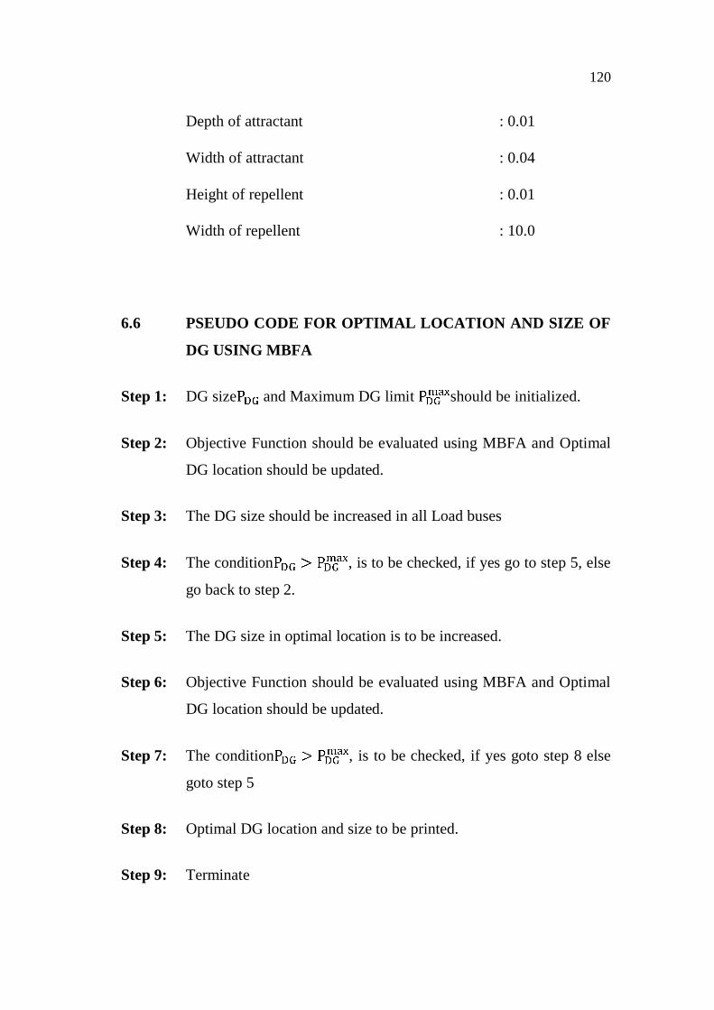
system. The rating of DG is varied between 1MW to 40 MW. Figure 6.3

shows the effect of DG placement on cost of power production on IEEE 14

bus system. From the figure, it is clear that the cost decreases when DG is

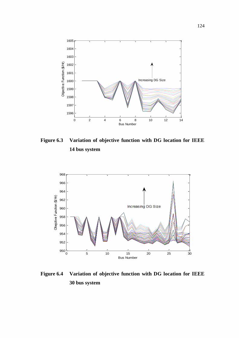
added at bus number 13. Similarly the optimal placement of DG for IEEE 30

bus system with increased loading of 30MW at bus number 2 is computed and

the results obtained are presented in Figure 6.4. From the figure, it is apparent

that the best cost minimization is obtained at bus number 7.

124

Figure 6.3 Variation of objective function with DG location for IEEE

14 bus system

Figure 6.4 Variation of objective function with DG location for IEEE

30 bus system

0 2 4 6 8 10 12 14

1596

1597

1598

1599

1600

1601

1602

1603

1604

1605

Bus Number

Increasing DG Size

0 5 10 15 20 25 30950

952

954

956

958

960

962

964

966

968

Bus Number

125

6.7.2 Optimal Size of DG

From the above discussion it is found that minimum OF is attained

when DG is placed at bus no 13 and bus number 7 for IEEE 14 and IEEE 30

bus system respectively. However, to identify the optimal rating of DG, for

reduced losses, now DG rating is increased between 1MW to 40MW in the

above identified optimal location. The results obtained for IEEE14 bus system

by connecting DG at bus no 7 is presented in Figure 6.5. Similarly the

variation of objective function with respect to change in DG size at optimal

location for IEEE30 bus system and 30 MW loading at bus number 2 is

shown in Figure 6.6. From the results presented in Figure 6.5 and 6.6, the

optimal values of DG are15 MW and 23 MW respectively.

Figure 6.5 Variation of objective function with DG size for IEEE

14 bus system at optimal location (bus no.13)

0 5 10 15 20 25 30 35 401596

1596.5

1597

1597.5

1598

1598.5

1599

1599.5

DG Size (MW)

126

Figure 6.6 Variation of objective function with DG size for IEEE 30

bus system at optimal location (bus no.7)

To test the effectiveness of the proposed algorithm, different levels

of loading was done at randomly selected PQ buses. The results obtained are

tabulated and presented in Table 6.3. From the table, it is observed that, when

30MW additional loading is done at buses 2, 4, 14, 17 and 10, the

corresponding optimal DG locations are found to be bus no 21, 7, 24, 9 and

22 respectively.

Further, it may be noted that, the rating of DG added to meet the

additional load is always less than that of the load increased; because of the

fact that, in the practical case, DGs are located closer to the demand point so

that it meets the required amount of additional load. However, the addition of

DG to the existing IEEE14 and IEEE30 bus system will contribute to increase

in total generation cost. This increased cost can be met with savings made in

loss reduction. It is also seen from the table that, in most of the cases, bus

number above 20 is found to be the optimal location.

127

Table 6.3 Optimal sizing and location of DG devices under variable

loading conditions

Bus No.

Normal Loading

New Loading

Optimal DG size

Optimal DG

Location

Total loss

Total Cost

Total Load

MW MW MW Bus No. MW $/Hr MW 30 MW loading

02 21.7 51.7 22.00 21 7.964 951.1 313.4

04 07.6 37.6 23.87 07 8.272 953.2 313.4

14 06.2 36.2 23.98 24 9.615 956.9 313.4

17 09.0 39.0 28.16 09 8.94 955.8 313.4

10 05.8 35.8 26.00 22 8.879 955.0 313.4

20 MW loading

15 08.2 28.2 18.18 19 8.575 919.7 303.4

15 MW loading

18 03.2 18.2 12.54 10 9.119 903.8 298.4

10 MW loading

20 02.2 12.2 8.188 27 8.755 885.3 293.4

23 03.2 13.2 7.733 06 9.021 886.0 293.4

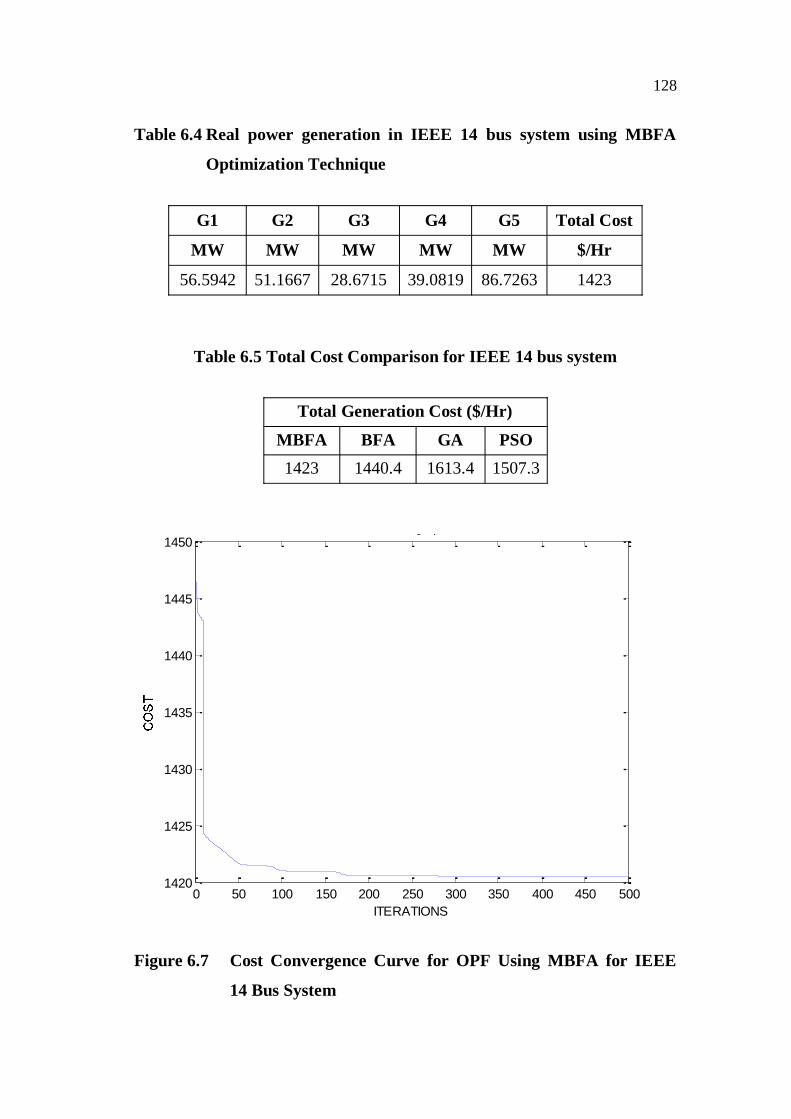
6.7.3 OPF without DG in IEEE 14 Bus System

The real power generations in IEEE 14 bus system under normal

loading conditions without including DG is given in Table 6.4. The total

generation cost including the cost of DG for a IEEE 14 bus system is found to

be 1423$/Hr using the proposed MBFA algorithm. This generation cost is

compared with other optimization techniques namely BFA, GA and PSO in

Table 6.5. The cost convergence curve for OPF Using MBFA in IEEE-14 Bus

System is shown in Figure 6.7. From the figure it is clear that the approximate

convergence takes near 52nd iteration.

128

Table 6.4 Real power generation in IEEE 14 bus system using MBFA

Optimization Technique

G1 G2 G3 G4 G5 Total Cost

MW MW MW MW MW $/Hr

56.5942 51.1667 28.6715 39.0819 86.7263 1423

Table 6.5 Total Cost Comparison for IEEE 14 bus system

Total Generation Cost ($/Hr)

MBFA BFA GA PSO 1423 1440.4 1613.4 1507.3

Figure 6.7 Cost Convergence Curve for OPF Using MBFA for IEEE

14 Bus System

0 50 100 150 200 250 300 350 400 450 5001420

1425

1430

1435

1440

1445

1450MBFA graph

ITERATIONS

129

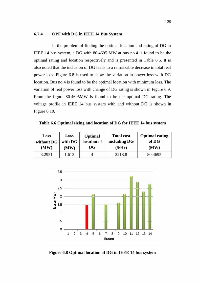
6.7.4 OPF with DG in IEEE 14 Bus System

In the problem of finding the optimal location and rating of DG in

IEEE 14 bus system, a DG with 80.4695 MW at bus no.4 is found to be the

optimal rating and location respectively and is presented in Table 6.6. It is

also noted that the inclusion of DG leads to a remarkable decrease in total real

power loss. Figure 6.8 is used to show the variation in power loss with DG

location. Bus no.4 is found to be the optimal location with minimum loss. The

variation of real power loss with change of DG rating is shown in Figure 6.9.

From the figure 80.4695MW is found to be the optimal DG rating. The

voltage profile in IEEE 14 bus system with and without DG is shown in

Figure 6.10.

Table 6.6 Optimal sizing and location of DG for IEEE 14 bus system

Loss without DG

(MW)

Loss with DG

(MW)

Optimal location of

DG

Total cost including DG

($/Hr)

Optimal rating of DG (MW)

3.2951 1.613 4 2218.8 80.4695

Figure 6.8 Optimal location of DG in IEEE 14 bus system

0

0.5

1

1.5

2

2.5

3

3.5

1 2 3 4 5 6 7 8 9 10 11 12 13 14Bus no

130

Figure 6.9 Power Loss variations with DG size in IEEE 14 bus system under normal loading condition

Figure 6.10 Voltage profile with and without DG in IEEE14 bus system

0 50 100 150 200 250 300 3500

2

4

6

8

10

12

14

16

18Loss variation at DG located bus

DG size

0 2 4 6 8 10 12 141.01

1.02

1.03

1.04

1.05

1.06

1.07

1.08

1.09

1.1

1.11VOLTAGE PROFILE

BUS NO.

131

6.7.5 OPF without DG in IEEE 30 Bus System

The total generation cost including the cost of DG for a IEEE 30

bus system using the proposed MBFA technique is found to be 798.22$/Hr.

This generation cost is compared with other optimization techniques namely

BFA, GA and PSO in Table 6.7. The cost convergence curve for OPF Using

MBFA in IEEE 30 Bus System is shown in Figure 6.7. From the figure it is

evident that the objective function converges at 35th iteration.

Table 6.7 Total Cost Comparison for IEEE 30 bus system

Total generation cost ($/Hr) MBFA BFA GA PSO

798.2 800.2052 803.5495 801.26

Figure 6.11 Cost Convergence Curve for OPF Using MBFA in IEEE 30

Bus System

0 10 20 30 40 50 60 70 80 90 100798

799

800

801

802

803

804

805

806

807

808

ITERATIONS

132

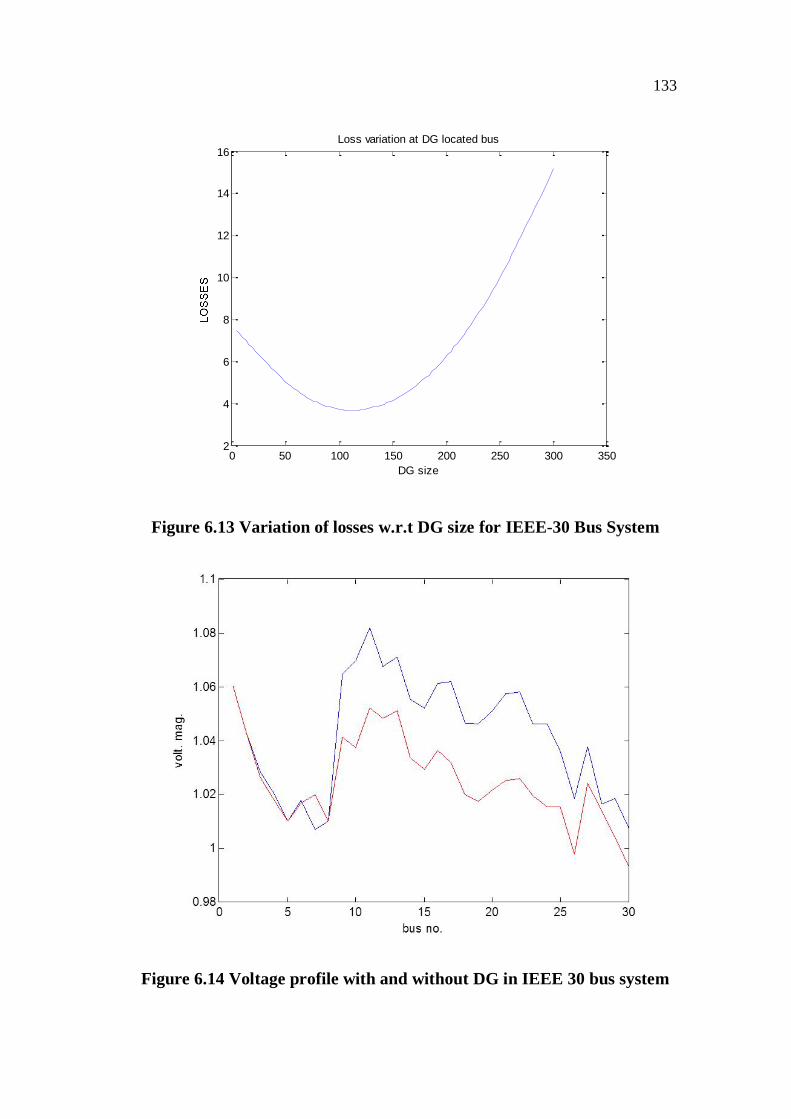
6.7.6 OPF with DG in IEEE 30 Bus System

In the problem of finding the optimal location and rating of DG in

IEEE 30 bus system, a DG with 128.823 MW at bus no.6 is found to be the

optimal rating and location respectively and is presented in Table 6.8. It is

also noted that the inclusion of DG leads to a remarkable decrease in total real

power loss of 5MW. Figure 6.12 is used to show the variation in power loss

with DG location. Bus no.6 is found to be the optimal location with minimum

loss. The variation of real power loss with change of DG rating is shown in

Figure 6.13. From the figure 128.8223MW is found to be the optimal DG

rating. The voltage profile in IEEE 30 bus system with and without DG is

shown in Figure 6.14.

Table 6.8 optimal sizing and location of DG for IEEE 30 bus system

Loss without

DG (MW)

Loss with DG

(MW)

Optimal location of DG

Total cost including DG

($/Hr)

Optimal rating of DG

(MW) 7.4016 2.437 6 2694.9 128.8223

Figure 6.12 Optimal location of DG in IEEE 30 bus system

0

1

2

3

4

5

6

7

8

1 3 5 7 9 11 13 15 17 19 21 23 25 27 29Bus no

133

Figure 6.13 Variation of losses w.r.t DG size for IEEE-30 Bus System

Figure 6.14 Voltage profile with and without DG in IEEE 30 bus system

0 50 100 150 200 250 300 3502

4

6

8

10

12

14

16Loss variation at DG located bus

DG size

134

6.7.7 OPF including DG under Variable Loading Condition

The proposed MBFA method for solving OPF including DG is

further analyzed under variable condition. An increased loading of 50MW,

40MW and 30MW is done on all buses except slack and PV buses and the

optimal location and rating of DG for this variable loading is obtained. The

corresponding total real power loss is also monitored. Table 6.9, Table 6.10

and Table 6.11 presents the optimal rating of DG, optimal location of DG and

total real power loss under 50MW, 40MW and 30MW respectively.

The total real power loss variation under each iteration in a IEEE

30 bus system for and increased loading of 50MW, 40MW and 30MW are

shown in Figure 6.15, Figure 6.16 and Figure 6.17 respectively. The voltage

profile in IEEE 30 bus system with and without DG for an increased loading

of 50MW, 40 MW and 30MW are shown in Figure 6.18, Figure 6.19 and

Figure 6.20 respectively.

Figure 6.21 shows the variation of total real power loss with change

in DG rating for 50MW increased loading in optimal DG location i.e bus

no.14. The optimal rating obtained is 78.96MW and the corresponding loss is

6.15MW. Similarly for 40 MW and 30MW increased loading, the optimal

rating is found to be 69.50MW with 6.34MW loss and 82.69MW with

5.42MW loss respectively and is shown in Figure 6.22 and Figure 6.23.

135

Table 6.9 Optimal rating and location of DG and Corresponding Losses

in IEEE-30 Bus system for 50MW increased loading

Bus No.

Load Optimal DG Power Loss Before After Size Location

(MW) (MW) (MW) (Bus No.) (MW)

3 2.4 52.4 140.71 9 4.12

4 7.6 57.6 167.844 4 3.88

6 0 50 127.96 6 3.88

7 22.8 72.8 137.01 7 3.60

9 0 50 158.64 9 3.18

10 5.8 55.8 162.75 9 3.1817

12 11.2 61.2 116.12 6 4.54

14 6.2 56.2 78.96 14 6.51

15 8.2 58.2 109.65 15 5.55

16 3.5 53.5 122.84 6 5.06

17 9 59 166.29 9 4.70

18 3.2 53.2 89.07 18 5.144

19 9.5 59.5 93.45 19 5.52

20 2.2 52.2 98.37 20 5.84

21 17.5 67.5 118.81 21 4.61

22 0 50 166.06 9 4.61

23 3.2 53.2 93.08 23 6.15

24 8.7 58.7 100.21 24 5.93

27 0 50 176.55 6 4.90

28 0 50 124.37 6 4.63

136

Table 6.10 Optimal rating and location of DG and Corresponding

Losses in IEEE-30 Bus system for 40MW increased loading

Bus No.

Load Optimal DG Power Loss Before After Size Location

(MW) (MW) (MW) (Bus No.) (MW)

3 2.4 42.4 135.30 9 3.88

4 7.6 47.6 164.88 4 4.07

6 0 40 148.36 9 4.36

7 22.8 62.8 129.38 7 3.54

9 0 40 152.07 9 3.71

10 5.8 45.8 155.53 9 3.33

12 11.2 51.2 96.16 6 3.43

14 6.2 46.2 154.43 4 6.49

15 8.2 48.2 99.39 15 5.19

16 3.5 43.5 147.22 9 5.37

17 9 49 153.49 9 4.08

18 3.2 43.2 81.48 18 5.43

19 9.5 49.5 83.98 19 5.94

20 2.2 42.2 90.54 20 5.28

21 17.5 57.5 152.05 9 4..38

22 0 40 151.33 9 3.96

23 3.2 43.2 79.32 23 5.57

24 8.7 48.7 87.63 24 5.12

27 0 40 143.03 6 4.34

28 0 40 109.60 6 4.52

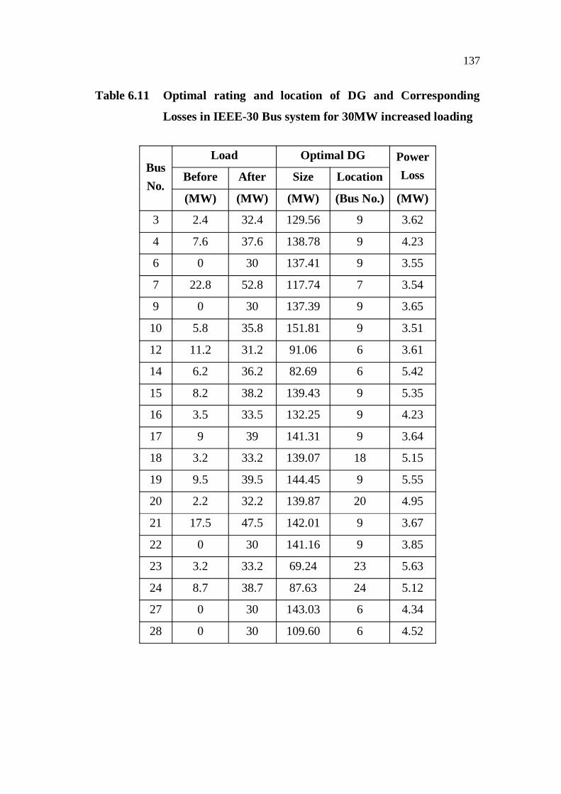
137

Table 6.11 Optimal rating and location of DG and Corresponding

Losses in IEEE-30 Bus system for 30MW increased loading

Bus No.

Load Optimal DG Power Loss Before After Size Location

(MW) (MW) (MW) (Bus No.) (MW)

3 2.4 32.4 129.56 9 3.62

4 7.6 37.6 138.78 9 4.23

6 0 30 137.41 9 3.55

7 22.8 52.8 117.74 7 3.54

9 0 30 137.39 9 3.65

10 5.8 35.8 151.81 9 3.51

12 11.2 31.2 91.06 6 3.61

14 6.2 36.2 82.69 6 5.42

15 8.2 38.2 139.43 9 5.35

16 3.5 33.5 132.25 9 4.23

17 9 39 141.31 9 3.64

18 3.2 33.2 139.07 18 5.15

19 9.5 39.5 144.45 9 5.55

20 2.2 32.2 139.87 20 4.95

21 17.5 47.5 142.01 9 3.67

22 0 30 141.16 9 3.85

23 3.2 33.2 69.24 23 5.63

24 8.7 38.7 87.63 24 5.12

27 0 30 143.03 6 4.34

28 0 30 109.60 6 4.52

138

Figure 6.15 Loss variation in DG installed bus under 50 MW loading

Figure 6.16 Loss variation in DG installed bus under 40 MW loading

0 10 20 30 40 50 60 70 80 90 1005

6

7

8

9

10

11

12

13

14Loss variation at DG located bus

ITERATIONS

139

Figure 6.17 Loss variation in DG installed bus under 30 MW loading

Figure 6.18 Voltage profile with and without DG for 50 MW increased

loading

0 5 10 15 20 25 300.95

1

1.05

1.1VOLTAGE PROFILE

BUS NO.

140

Figure 6.19 Voltage profile with and without DG for 40 MW increased

loading

Figure 6.20 Voltage profile with and without DG for 30 MW increased

loading

0 5 10 15 20 25 300.98

1

1.02

1.04

1.06

1.08

1.1

1.12VOLTAGE PROFILE

BUS NO.

0 5 10 15 20 25 300.98

1

1.02

1.04

1.06

1.08

1.1VOLTAGE PROFILE

BUS NO.

141

Figure 6.21 Loss variations with DG size in IEEE 30 bus system under

50 MW increased loading

Figure 6.22 Loss variations with DG size in IEEE 30 bus system under

40 MW increased loading

0 50 100 150 200 250 300 3500

10

20

30

40

50

60

70Loss variation at DG located bus

DG SIZE

0 50 100 150 200 250 300 3500

10

20

30

40

50

60

70Loss variation at DG located bus

DG SIZE

142

Figure 6.23 Loss variations with DG size in IEEE 30 bus system under 30 MW increased loading

6.8 CONCLUSION

In this work, Modified Bacterial Foraging Optimization Algorithm

is proposed to find the optimal location and sizing of DG for IEEE14 and

IEEE30 bus system. Minimization of total cost, in addition to optimal location

and sizing of DG, is framed as objective function and solved using the

proposed method. Further, the proposed method is tested under varying load

conditions and the results are presented. From the results, it is apparent that,

appropriate size and location of DG sources are highly crucial, and important

to maximize the benefits. The proposed algorithm is found to be effective in

finding the optimal DG size and location and the suitable DG sizes are 15MW

and 23MW for IEEE14 with increased loading of 30MW in bus number 4 and

IEEE30 bus system with increased loading in bus number 2 respectively.

Finally, the results obtained in this study, demonstrated that DG is a viable

economic alternative relative to upgrading substations and feeder facilities, if

the incremental cost of serving additional load is considered.

0 50 100 150 200 250 300 3504

5

6

7

8

9

10

11

12Loss variation at DG located bus

DG SIZE