134 CHAPTER 6 SEGMENTATION OF EXUDATES Like hemorrhages, exudates are also the pathological features in DR. The segmentation of exudates also greatly helps in automatic screening system. The exudates are precipitations of plasma protein in the retinal region and appear as bright, reflective, white or cream-colored lesions on the retinal image. The exudates are a developed stage from microaneurysms and hemorrhages. The vision loss is inevitable, if it is ignored. The segmentation of the exudates is carried out using various clustering techniques and the results are presented and discussed elaborately in this chapter. The images from the standard database are used for testing, validating and measure the performance of the proposed technique. The relative merits of each clustering technique have been presented. The segmentation of exudates will be successful only when the OD is eliminated from the retinal image as it has more or less equal brightness. Detection of the OD center and OD boundary using vessel-direction matched filter and masking of OD have been explained in the Chapter 4. In this process, the images with OD detection and elimination by masking techniques are used as input images. OD masked image is subjected to further processing to segment the exudates. As exudates are the bright region, Hussain et al (2010) and Giancardo et al (2011) applied the thresholding technique to segment the exudates.
Transcript
134
CHAPTER 6
SEGMENTATION OF EXUDATES
Like hemorrhages, exudates are also the pathological features in
DR. The segmentation of exudates also greatly helps in automatic screening
system. The exudates are precipitations of plasma protein in the retinal region
and appear as bright, reflective, white or cream-colored lesions on the retinal
image. The exudates are a developed stage from microaneurysms and
hemorrhages. The vision loss is inevitable, if it is ignored.
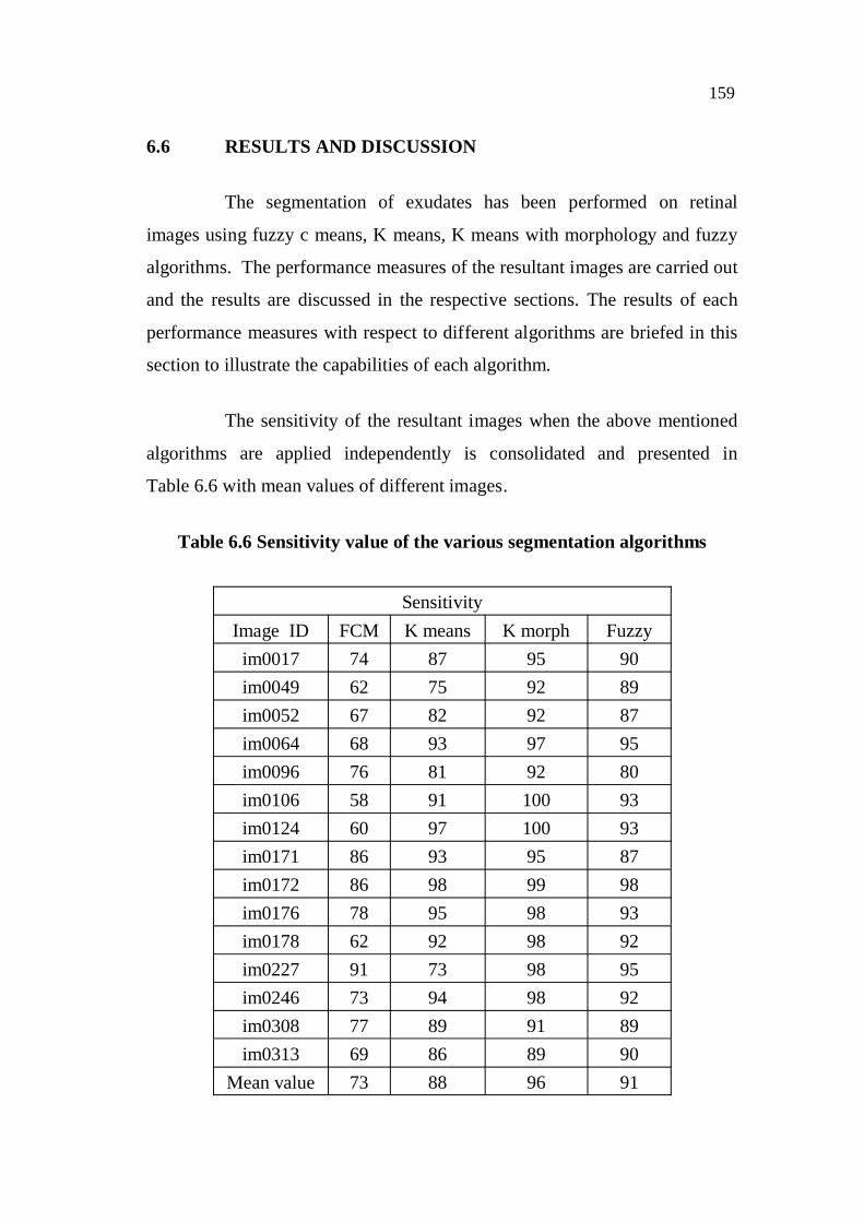
The segmentation of the exudates is carried out using various
clustering techniques and the results are presented and discussed elaborately
in this chapter. The images from the standard database are used for testing,
validating and measure the performance of the proposed technique. The
relative merits of each clustering technique have been presented.
The segmentation of exudates will be successful only when the OD
is eliminated from the retinal image as it has more or less equal brightness.
Detection of the OD center and OD boundary using vessel-direction matched
filter and masking of OD have been explained in the Chapter 4. In this
process, the images with OD detection and elimination by masking
techniques are used as input images. OD masked image is subjected to further
processing to segment the exudates. As exudates are the bright region,
Hussain et al (2010) and Giancardo et al (2011) applied the thresholding
technique to segment the exudates.
135
In th
resh
oldi
ng te
chni
que,
the
thre
shol
d va
lue
of th
e im
age
is s
et a
s
one
or m
ore
than
one
. If
thre
shol
d va
lue
is s
et a
s on
e, t
he i
mag
e w
ill b
e
divi
ded
into
two
regi
ons
as e
xpla
ined
in C
hapt
er 4
, Sec
tion
4.1.
2. I
n re
tinal
imag
es,
the
thre
shol
d va
lues
can
not
be f
ixed
eas
ily a
s th
ey h
ave
diff
eren
t
inte
nsity
lev
els.
Furth
er,
it w
ill n
ot b
e un
iform
. H
ence
, th
e th
resh
oldi
ng
tech
niqu
e is
not
abl
e to
yie
ld s
atis
fact
ory
resu
lts.
In o
rder
to
achi
eve
the
segm
enta
tion
proc
ess s
ucce
ssfu
lly, v
ario
us c
lust
erin
g te
chni
ques
like
Fuz
zy C
Mea
ns
(FC
M),
K
mea
ns
clus
terin
g,
com
bina
tion
of
K
mea
ns
with
mor
phol
ogy
and
fuzz
y ar
e us
ed i
n se
gmen
tatio
n pr
oces
s. Th
e pr
opos
ed
clus
terin
g te
chni
ques
are
app
lied
over
the
OD
mas
ked
imag
es a
fter c
onve
rting
them
into
gra
y sc
ale
imag
es. T
he e
ntire
pro
cess
is s
chem
atic
ally
illu
stra
ted
as
bloc
k di
agra
m in
Fig
ure
6.1.
Figu
re 6
.1 B
lock
dia
gram
for
exud
ates
segm
enta
tion
OD
mas
ked
Retin
al Im
age
RG
B to
gra
y K m
eans
and
m
orph
olog
y Fu
zzy
C M
eans
Fu
zzy
Exud
ates
Seg
men
tatio
n an
d Pa
ram
etric
Mea
sure
s
Km
eans
136
6.1
CL
UST
ER
ING
TE
CH
NIQ
UE
S
The
clus
terin
g te
chni
que
uses
int
ensi
ty r
elat
ions
hip
amon
g th
e pi
xels
of
an i
mag
e. I
t cla
ssifi
es th
e pi
xels
int
o di
ffer
ent g
roup
s ba
sed
on it
s in
tens
ity. I
n a
parti
cula
r gr
oup,
sim
ilarit
y m
easu
rem
ents
am
ong
the
pixe
ls a
re
carr
ied
out a
nd d
epen
ding
on
thei
r val
ue, t
he p
ixel
s will
be
clus
tere
d. A
mon
g th
e va
rious
clu
ster
s, th
e si
mila
rity
leve
l w
ill b
e va
ryin
g w
here
as i
n th
e pa
rticu
lar
clus
ter
the
sim
ilarit
y va
lue
will
be
mor
e or
less
the
sam
e w
ithou
t m
uch
varia
tion.
A s
tand
ard
proc
edur
e fo
r as
sign
ing
a pi
xel
to th
e cl
uste
r is
ba
sed
on th
e m
ean
valu
e of
the
pixe
ls p
rese
nt in
the
clus
ter.
Ach
ievi
ng s
uch
a gr
oupi
ng r
equi
res
a si
mila
rity
met
ric th
at in
volv
es th
e in
put
vect
ors
and
its
valu
e re
flect
s the
ir si
mila
rity
Jeya
ram
an (2
012)
.
In o
rder
to
achi
eve
bette
r re
sult,
the
RG
B c
olor
im
ages
are
co
nver
ted
into
gra
y sc
ale
imag
es a
nd re
duce
d in
to 2
56 X
256
siz
e be
fore
the
appl
icat
ion
of th
e cl
uste
ring
tech
niqu
e. T
his
proc
ess
will
ena
ble
one
to o
btai
n re
sults
in
a sh
ort
time
as t
hese
pro
cess
es a
re i
tera
tive
ones
. C
onve
rsio
n of
R
GB
col
or s
pace
to g
ray
scal
e is
exp
lain
ed in
Cha
pter
4, S
ectio
n 4.
1.1.
1. T
he
vario
us c
lust
erin
g te
chni
ques
are
dis
cuss
ed i
n th
e fo
llow
ing
sect
ions
in
a se
quen
tial m
anne
r.
6.2
FUZ
ZY
C M
EA
NS
CL
UST
ER
ING
(FC
M)
It is
a d
ata
clus
terin
g al
gorit
hm a
nd it
clu
ster
s th
e pi
xel b
ased
on
its
mem
bers
hip
grad
e in
to d
iffer
ent c
lust
ers.
The
vario
us s
teps
inv
olve
d in
this
137
(a)
(b)
(c)
(d)
138
The images with various clusters contain useful information based
on their grouping. From the above resultant image, the first cluster shows the
exudates clearly compared with the other clusters as the intensity level of the
exudates matches with the first cluster. In most of the tested images, the
exudates are segmented in first cluster only. However, it is not necessary that
in all the images the exudates will be segmented in the first cluster. The
segmentation process basically depends on the intensity of the exudates
corresponding to the clusters. In other clusters, the features like blood vessels
and optic disc are also segmented. The 1st cluster image is considered as the
segmented output of exudates. The algorithm is tested with images of STARE
database and the parametric measures are carried out. The results are
presented in Table 6.1 with image identification number, TP, FP, FN, TN, SE,
SPE, ACC and processing time in seconds.
Table 6.1 Parametric measures of the fuzzy c means method
FUZZY C MEANS Sl.No. Image ID Number of Pixels Percentage Time
From the results, it is inferred that the mean values of SE, SPE,
ACC and time in seconds are estimated as 73%, 97%, 95% and 9.5 sec
respectively. The FCM method has the highest specificity of 97% and
accuracy of 95%. However, the sensitivity is relatively lower as 73%. Hence,
it is attempted to increase the sensitivity using various other algorithms. In
continuation of this algorithm, K means clustering technique is adopted and
the various steps involved are briefed in the next section.
6.3 K MEANS CLUSTERING ALGORITHM
It is one of the clustering techniques that classify a given data set to
a certain fixed number of clusters based on the similarity of the pixels or
group of pixels. The fixed number of clusters is assumed as ‘K’. Unlike in the
previous technique, membership grade of the pixel is not considered in this
algorithm. Instead, it classifies each pixel in a group with the closest mean
distance between the centroid and the pixel. It is an iterative procedure and
this algorithm clusters the data iteratively by computing a mean intensity for
each group and the various steps involved in this algorithm are given below.
Step 1 : Provide the input data and number of clusters
Step 2 : Calculate the cluster centroids based on assumed initial
value
Step 3 : Calculate the distance of each pixel from class centroid
Step 4 : Group pixels into k clusters based on minimal distance
from centroids
Step 5 : Calculate new centroid for each cluster
Step 6 : Classify into groups based on new centroid and distance
Step 7 : Test if any centroid changes its position.
140
Step 8 : If there are changes repeat step 3- 8, else go to step 9
Step 9 : End
The above steps are illustrated as a flow diagram in Figure 6.3.
Figure 6.3 Flow chart for K means clustering technique
In this method, if there are ‘K’ number of clusters, the number of
centroids or cluster centers are also ‘K’ corresponding to each cluster. The
centroid for a cluster is based on the range of intensity values present in a
particular cluster. Usually, it is assumed as the mean value of the variation
range corresponding to the intensity levels. At the beginning stage, these
centroids are fixed at suitable positions and they are iterated towards the exact
location in the process.
No
Yes
Number of Cluster K Number of Cluster K
Start
End
Distance between the objects and Centroids
Centroid
Grouping Based on minimum distance
Object Move to the
Group
Number of Cluster K
141
The pixels present in the original image are transferred to different clusters based on their intensity value. This algorithm predicts a cluster center in each group so that a cost function (objective function) of dissimilarity (distance) measure is minimized. Euclidean distance is a measure of distance between the pixel intensity and the cluster center. It is used for calculating the error function. The equation for error function in terms of euclidean distance for the pixels contained in cluster is given in Equation (6.1). Finally, this algorithm aims at minimizing a squared error objective function (J).
2)(
1 1j
ji
k
j
n
i
cxJ (6.1)
where,
2)(j
ji cx - Euclidean distance measure between a data point
‘ ix ’belonging to cluster j and its cluster centre ‘ jc ’.
If a pixel has a value corresponding to the nearest value of the centroid of the particular cluster, it is transferred to that cluster. This process continues till all the pixels are grouped into any one of the clusters that are assumed to be initial clusters. Further, the centroids of the clusters are iterated towards the better values within the cluster. The above step is repeated until no pixel is moving from one cluster to another. When the step reaches this point, if the clusters are stable, the clustering process stops.
Usually, exudates are the high intensity pixel regions in the retinal image. Based on this property, this clustering technique is applied to segment the exudates in the retinal images. OD masked image is adopted for the K means clustering algorithm and is separated into five clusters based on the intensities in the image. Resultant clusters after the application of the K means clustering on STARE database image with an identification number im0049 are shown in Figures.6.4 (a) to (f). Figures 6.4 (a),(b),(c),(d) and (e) show the resultant images of five different clusters with various intensity levels.
142
(a) (b)
(c) (d)
(e) (f)
Figure 6.4 Resultant output of K means clustering technique (a) output of cluster1 (b) output of cluster 2 (c) output of cluster 3 (d) output of cluster 4 (e) output of cluster 5 (f) post processed output
143
The resultant images of the clusters shown in Figures 6.4 (d) and
(e) have segmented the exudates in comparison with other clusters. However,
Figure 6.4 (d) has segmented even small exudates compared to Figure 6.4 (e).
As a result, Figure 6.4 (d) is suitable for further processing to fill the image
regions and holes (contour of bright pixels contained darker region within the
boundary). The filling of the holes is achieved by filling bright pixels in the
holes.
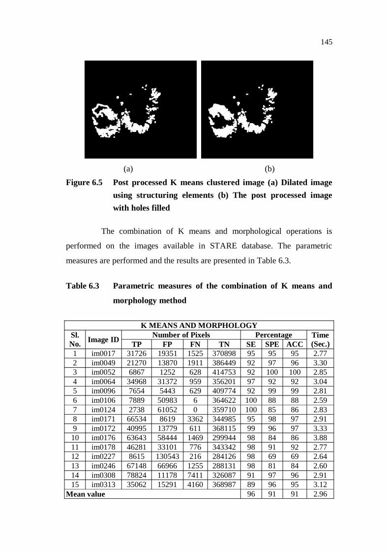
The image with holes filled is shown in Figure 6.4 (f) and the
image with the segmented exudates is considered as output using K means
clustering technique. Similar to FCM, K means clustering algorithm is
implemented in the exudates images in the STARE database and the predicted
SE , SPE, ACC and the processing time of are tabulated in Table 6.2.
Table 6.2 Parametric measures of the K means clustering method
K MEANS Sl.No. Image ID Number of Pixels Percentage Time