Chapter 6. SYSTEM SIMULATION

Min Soo KIM

Department of Mechanical and Aerospace EngineeringSeoul National University

Optimal Design of Energy Systems (M2794.003400)

Chapter 6. SYSTEM SIMULATION

- Calculation of operating variables(pressure, temp., flow rate, etc…) in a thermal system operating in a steady state.

- To presume performance characteristics and equations for thermodynamic properties of the working substances.

6.1 Description of system simulation

System System simulation


A

C

BD

① ②

④ ③

Mass balanceEnergy balance

①-② : Mathematic equations


②-③ : Mathematic equations


③-④ : Mathematic equations


④-① : Mathematic equations

Solutions

calculation

• a set of simultaneous equations• characteristics of all components• thermodynamic properties

6.2 Some uses of simulation


Part load

Overload

Cost of energy

engineer

Pressures

Temperatures

Flow rates

Operation variables

Pumps

Compressors

Heat exchangers

Components

Turbines

choose

normal operation

Design stage – to achieve improved design

Existing system – to explore prospective modifications

Design condition

Off design condition (part load / over load)

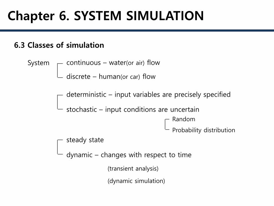
6.3 Classes of simulation


continuous – water(or air) flow

discrete – human(or car) flow

deterministic – input variables are precisely specified

stochastic – input conditions are uncertain

steady state

dynamic – changes with respect to time

(transient analysis)

(dynamic simulation)

Random

Probability distribution

System

6.4 Information-flow diagrams


- A block signifies that an output can be calculated when the input is known

w, flow rate

𝑝1

𝑝2

(a)

Pump

𝑓 𝑝1, 𝑝2, 𝑤 = 0

Pump

𝑓 𝑝1, 𝑝2, 𝑤 = 0

𝑝1

𝑝2𝑤

𝑝1𝑝2

𝑤

(b)

Fig. (a) Centrifugal pump in fluid-flow diagram (b) possible information-flow blocksrepresenting pumps.

or

Fluid

Energyfinput output

transferfunction


𝑓1 𝑤𝐴, 𝑝3 = 0

𝑓2 𝑤𝐵, 𝑝4 = 0

𝑓3 𝑤1, 𝑝1 = 0

𝑓4 𝑤1, 𝑝2, 𝑝3 = 0

𝑓5 𝑤2, 𝑝3, 𝑝4 = 0

Fig. (a) Fire-water system (b) pump characteristics.

(a) (b)

𝑤

𝑝2−𝑝1

𝑓 𝑝1, 𝑝2, 𝑤 = 0

pump characteristics

𝑝at𝑚

𝑤𝐴 𝑤𝐵

Hydrant A Hydrant B

3 412

0

𝑤2𝑤1

ℎ m

𝑤𝐴 = 𝐶𝐴 𝑝3 − 𝑝atm

𝑤𝐵 = 𝐶𝐵 𝑝4 − 𝑝atm

𝑝atm − 𝑝1 = 𝐶1𝑤12 + 𝜌𝑔ℎ

𝑝2 − 𝑝3 = 𝐶2𝑤12

𝑝3 − 𝑝4 = 𝐶3𝑤22

Section 0-1 :

Section 1-2 :

Section 2-3 :


Fig. Information-flow diagram for fire-water system.

𝑓6 𝑤1, 𝑝1, 𝑝2 = 0

𝑓7 𝑤1, 𝑤𝐴, 𝑤2 = 0

𝑓8 𝑤2, 𝑤𝐵 = 0

𝑤1 = 𝑤𝐴 + 𝑤2


Pump characteristics :

Mass balance : or

𝑤2 = 𝑤𝐵or

Pump

𝑓6 𝑤1, 𝑝1, 𝑝2

Pipe𝑓3 𝑤1, 𝑝1

Mass balance

𝑓7 𝑤1, 𝑤𝐴, 𝑤2


Pump

𝑓6 𝑤1, 𝑝1, 𝑝2


Pump𝑓6 𝑤1, 𝑝1, 𝑝2

Mass balance𝑓8 𝑤2, 𝑤𝐵

𝑤𝐴

𝑤1𝑝1𝑝2

𝑤2

𝑤𝐵

𝑝3

𝑝4


6.5 Sequential and simultaneous calculations

input outputinput

output𝑓1 𝑓2

Sequential calculation

Simultaneous calculations

𝑓1 𝑓2

𝑓4 𝑓3


6.6 Two methods of simulation:


Successive substitution

Newton-Raphson

- To solve a set of simultaneous algebraic equations

- The successive substitution is a straight-forward technique and is closelyassociated with the information-flow diagram of the system.

- The Newton-Raphson method is based on a Taylor-series expansion.

- Each method has advantages and disadvantages

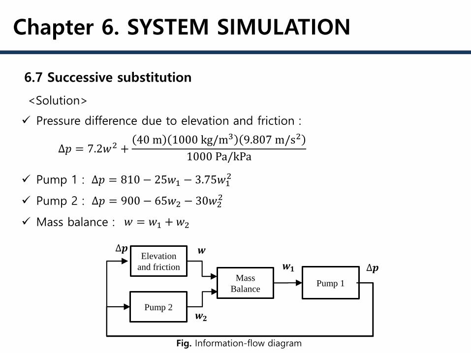
6.7 Successive substitution


𝑤2

𝑤140 m 𝑤

∆𝑝Fig. Water-pumping system

Pump 1: ∆𝑝 = 810 − 25𝑤1 − 3.75𝑤12 [kPa]

Pump 2: ∆𝑝 = 900 − 65𝑤2 − 30𝑤22 [kPa]

The friction in the pipe = 7.2𝑤2

<Example 6.1>

Determine the values ∆𝑝,𝑤1, 𝑤2 and 𝑤 by using successive substitution.

<Given>

- Assume a value of one or more variables and begin the calculation untilthe originally-assumed variables have been recalculated.

- The recalculated values are substituted successively, and the calculationloop is repeated until satisfactory convergence is achieved.



Elevation

and friction

Pump 2

Mass

BalancePump 1

∆𝒑

𝒘𝟏 ∆𝒑

𝒘

𝒘𝟐

Fig. Information-flow diagram

Pressure difference due to elevation and friction :

Pump 1 :

Pump 2 :

Mass balance :

<Solution>

∆𝑝 = 7.2𝑤2 +40 m 1000 kg/m3 9.807 m/s2

1000 Pa/kPa

∆𝑝 = 810 − 25𝑤1 − 3.75𝑤12

∆𝑝 = 900 − 65𝑤2 − 30𝑤22

𝑤 = 𝑤1 + 𝑤2



Iteration with initial assumption :

1 1

2 2

3

1 2 2

( )

( )

( )

( , )

p f w

w f p

w f p

w f w w

<Solution>

Iteration ∆𝑝 𝑤2 𝑤 𝑤1

1 638.85 2.060 5.852 3.792

2 661.26 1.939 6.112 4.174

3 640.34 2.052 5.870 3.818

4 659.90 1.946 6.097 4.151

︙ ︙ ︙ ︙ ︙

47 649.98 2.000 5.983 3.983

48 650.96 1.995 5.994 3.999

49 650.04 2.000 5.983 3.984

50 650.90 1.995 5.993 3.998

𝑤1 = 4.2

Divergence occurs

Diagram 2 Diagram 3

Iteration w1 [kg/s] w2 [kg/s] w [kg/s] Δp [kPa]

1 4.000 2.000 5.983 650.00

2 3.942 1.983 6.019 653.16

3 4.258 2.077 5.812 635.53

4 2.443 1.554 6.814 726.54

5 11.353 4.371 divergence 42.87

Iteration w1 [kg/s] w2 [kg/s] w [kg/s] Δp [kPa]

1 3.973 1.992 6.000 651.48

2 4.028 2.008 5.965 648.47

3 3.916 1.975 6.036 654.61

︙ ︙ ︙ ︙ ︙

9 divergence 8.811 951.23


6.7 Pitfalls in successive substitution

Elevation

and friction

Pump 1

Mass

BalancePump 2

∆𝒑

𝒘𝟐 ∆𝒑

𝒘

𝒘𝟏

initial assumption : 𝑤2 = 2.0 initial assumption : 𝑤 = 6.0

Pump 1

Pump 2

Mass

Balance

Elevation

and friction

∆𝒑

𝒘 ∆𝒑

𝒘𝟏

𝒘𝟐

Check the flow diagram in advance (Ch.14)

Divergence occurs

Near the point ( , , ( , ))a b z a b

6.9 Taylor-series expansion


- The Newton-Raphson method is based on a Taylor-series expansion.

𝑐0 = 𝑧(𝑎, 𝑏)

𝑐1 =𝜕𝑧(𝑎, 𝑏)

𝜕𝑥

𝑐2 =𝜕𝑧(𝑎, 𝑏)

𝜕𝑦

𝑐3 =1

2

𝜕2𝑧(𝑎, 𝑏)

𝜕𝑥2

𝑐4 =𝜕2𝑧(𝑎, 𝑏)

𝜕𝑥𝜕𝑦

𝑐5 =1

2

𝜕2𝑧(𝑎, 𝑏)

𝜕𝑦2

𝑧 = 𝑐0 + 𝑐1 𝑥 − 𝑎 + 𝑐2 𝑦 − 𝑏

+𝑐3 𝑥 − 𝑎 2+𝑐4 𝑥 − 𝑎 𝑦 − 𝑏 +𝑐5 𝑥 − 𝑎 2 +⋯

𝑧 = 𝑧(𝑥, 𝑦)

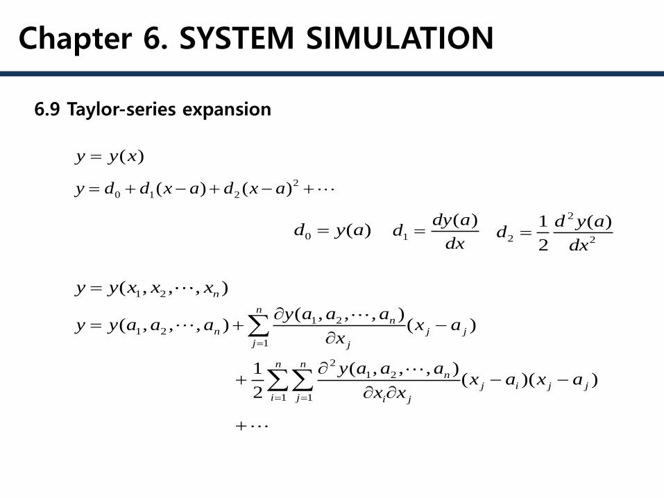
( )y y x

0 ( )d y a

2

0 1 2( ) ( )y d d x a d x a

1

( )dy ad

dx

2

2 2

1 ( )

2

d y ad

dx

1 2( , , , )ny y x x x

1 21 2

1

2

1 2

1 1

( , , , )( , , , ) ( )

( , , , )1( )( )

2

nn

n j j

j j

n nn

j i j j

i j i j

y a a ay y a a a x a

x

y a a ax a x a

x x



<Example 6.2> Express as a Taylor-series expansion at (x=2,y=1)

<Solution>

2ln( / )z x y

22 2

0 1 2 3 4 5ln ( 2) ( 1) ( 2) ( 2)( 1) ( 1)x

z c c x c y c x c x y c yy

2

0

2ln 1.39

1c

1 2

(2,1) 2 /1

/

z x yc

x x y

2 2

2 2

(2,1) /1

/

z x yc

y x y

2

3 2 2

1 (2,1) 1 2 1

2 2 4

zc

x x

2

4

(2,1)0

zc

x y

2

5 2 2

1 (2,1) 1 1 1

2 2 2

zc

y y

2 21 11.39 ( 2) ( 1) ( 2) ( 1)

4 2z x y x y



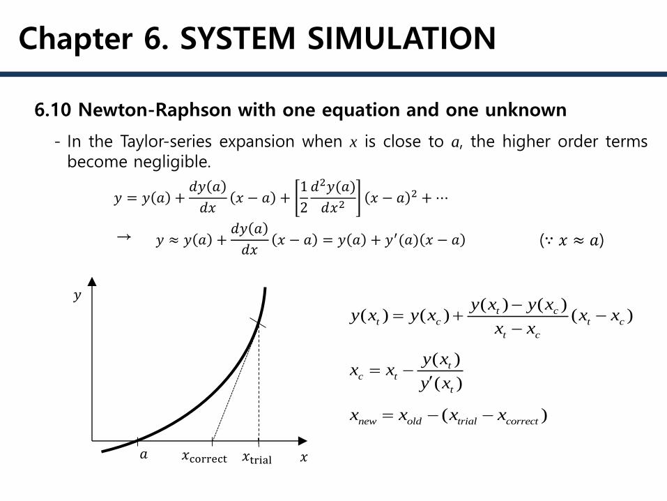
6.10 Newton-Raphson with one equation and one unknown


- In the Taylor-series expansion when x is close to a, the higher order termsbecome negligible.

→

𝑦 = 𝑦 𝑎 +𝑑𝑦 𝑎

𝑑𝑥𝑥 − 𝑎 +

1

2

𝑑2𝑦(𝑎)

𝑑𝑥2𝑥 − 𝑎 2 +⋯

(∵ 𝑥 ≈ 𝑎)

( ) ( )( ) ( ) ( )t c

t c t c

t c

y x y xy x y x x x

x x

( )

( )

tc t

t

y xx x

y x

( )new old trial correctx x x x

𝑎

𝑦

𝑥𝑥correct 𝑥trial

𝑦 ≈ 𝑦 𝑎 +𝑑𝑦 𝑎

𝑑𝑥𝑥 − 𝑎 = 𝑦 𝑎 + 𝑦′(𝑎) 𝑥 − 𝑎

Iteration xt y(x) y’(x) xc

1 2.000 -3.389 -6.389 1.470

2 1.470 -0.878 -3.347 1.207

3 1.207 -0.137 -2.345 1.149

4 1.149 -0.006 -2.154 1.146

5 1.146 0.000 -2.146

6.10 Newton-Raphson with one equation and one unknown


ex) 𝑦(𝑥) = 𝑥 + 2 − 𝑒𝑥 𝑦(𝑥𝑐) = 0

𝑥𝑡 = 2 𝑦 𝑥𝑡 = 𝑥𝑡 + 2 − 𝑒𝑥𝑡 = −3.39

𝑦 ≈ 𝑦 𝑥𝑐 + 𝑦′(𝑥𝑐) 𝑥 − 𝑥𝑐 𝑥𝑐 = 𝑥𝑡 −𝑦 𝑥𝑡𝑦′ 𝑥𝑡

= 2 −−3.39

1 − 𝑒2= 1.469 𝑥𝑡,𝑛𝑒𝑤

1 1 2 3

2 1 2 3

3 1 2 3

( , , ) 0

( , , ) 0

( , , ) 0

f x x x

f x x x

f x x x

trial value : 1 2 3, ,t t tx x x

1 1 2 31 1 2 3 1 1 2 3 1 1

1

1 1 2 32 2

2

1 1 2 33 3

3

( , , )( , , ) ( , , ) ( )

( , , )( )

( , , )( )

t t tt t t c c c t c

t t tt c

t t tt c

f x x xf x x x f x x x x x

x

f x x xx x

x

f x x xx x

x

2

3

f

f

6.11 Newton-Raphson with multiple equations and unknowns


1 1 11 1 1 1 2 3

1 2 3

2 2 22 2 2 1 2 3

1 2 3

3 3 3

3 3 3 1 2 3

1 2 3

( , , )

( , , )

( , , )

t c t t t

t c t t t

t c t t t

f f fx x f x x x

x x x

f f fx x f x x x

x x x

f f fx x f x x x

x x x

, , , ,( )i new i old i t i cx x x x →



2

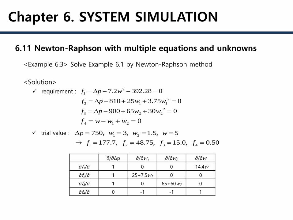
2 1 1810 25 3.75 0f p w w

2

1 7.2 392.28 0f p w

4 1 2 0f w w w

2

3 2 2900 65 30 0f p w w

1 2750, 3, 1.5, 5p w w w trial value :

requirement :

1 2 3 4177.7, 48.75, 15.0, 0.50f f f f →

∂/∂Δp ∂/∂w1 ∂/∂w2 ∂/∂w

∂f1/∂ 1 0 0 -14.4w

∂f2/∂ 1 25+7.5w1 0 0

∂f3/∂ 1 0 65+60w2 0

∂f4/∂ 0 -1 -1 1



<Solution>

<Example 6.3> Solve Example 6.1 by Newton-Raphson method

corrected variable :

1 2 3 498.84, 1.055, 0.541 1.096x x x x

1

2

3

4

1.0 0.0 0.0 72.0 177.7

1.0 47.5 0.0 0.0 48.75

1.0 0.0 155.0 0.0 15.0

0.0 1.0 1.0 1.0 0.50

x

x

x

x

, ,i i t i cx x x

1 2750 98.84 651.16 4.055, 2.041, 6.096p w w w

Iteration w1 [kg/s] w2 [kg/s] w [kg/s] Δp [kPa] f1 f2 f3 f4

1 3.000 1.500 5.000 750.00 177.720 48.750 15.000 0.500

2 4.055 2.041 6.096 651.16 -8.641 4.171 8.778 0.000

3 3.992 1.998 5.989 650.48 -0.081 0.015 0.056 0.000

4 3.991 1.997 5.988 650.49 0.000 0.000 0.000 0.000

1 2650.49, 3.991, 1.997, 5.988p w w w


<Solution>



6.13 Overview of system simulation

- The system simulation operate to achieve improved design or to exploreprospective modifications

- Choosing the combinations of dependent equation is important. But inlarge system is may not be simple to choose it.

- Successive substitution is a straight-forward technique and is usually easyto program. Its disadvantages are that sometimes the sequence may eitherconverge very slowly or diverge.

- The Newton-Raphson technique is based on a Taylor-series expansion. It ispowerful, but it is able to diverge on specific equations

Date post:	18-Dec-2021
Category:	Documents
Upload:	others
View:	2 times
Download:	0 times

Chapter 6. SYSTEM SIMULATION

Documents