Chapter 6 The Bow Shock and the Magnetosheath The solar wind plasma travels usually at speeds which are faster than any fluid plasma wave relative to the magnetosphere. Therefore a standing shock wave forms around the magnetosphere just as in front of an aircraft traveling at supersonic speeds. The bow shock is the shock in front of the magnetosphere and the magnetosheath is the shocked solar wind plasma. Therefore it is not directly the solar wind plasma which constitutes the boundary of the magnetosphere but the strongly heated and compressed plasma behind the bow shock. The region is rich in various wave phenomena, boundaries and shocks are often treated as discontinuities. 6.1 Solar Wind Solar coronal outflow: static atmosphere In a steady state with radial outflow the solar wind must satisfy continuity, momentum, and energy equations d dr r 2 nv = 0 (6.1) v dv dr = - GM r 2 - 1 m i n dp dr (6.2) d dr p n γ = 0 (6.3) with the gravitational constant G and the solar mass M . Exercise: Derive the above equation from the set of MHD equations The first solutions of these equations have assumed a static plasma (Chapman) yielding from (6.2) and (6.3) - GM r 2 - 1 m i n dp dr = 0 (6.4) d dr p n γ = 0 (6.5) 64
Transcript
Chapter 6
The Bow Shock and the Magnetosheath
The solar wind plasma travels usually at speeds which are faster than any fluid plasma wave relative tothe magnetosphere. Therefore a standing shock wave forms around the magnetosphere just as in frontof an aircraft traveling at supersonic speeds. The bow shock is the shock in front of the magnetosphereand the magnetosheath is the shocked solar wind plasma. Therefore it is not directly the solar windplasma which constitutes the boundary of the magnetosphere but the strongly heated and compressedplasma behind the bow shock. The region is rich in various wave phenomena, boundaries and shocksare often treated as discontinuities.
6.1 Solar Wind
Solar coronal outflow: static atmosphere
In a steady state with radial outflow the solar wind must satisfy continuity, momentum, and energyequations
d
dr
(r2nv
)= 0 (6.1)
vdv
dr= −GM
r2− 1
min
dp
dr(6.2)
d
dr
(p
nγ
)= 0 (6.3)
with the gravitational constant G and the solar mass M .
Exercise: Derive the above equation from the set of MHD equations
The first solutions of these equations have assumed a static plasma (Chapman) yielding from (6.2)and (6.3)
−GMr2− 1
min
dp
dr= 0 (6.4)
d
dr
(p
nγ
)= 0 (6.5)
64
CHAPTER 6. THE BOW SHOCK AND THE MAGNETOSHEATH 65
The energy equation can be written as
d
dr
(p
nγ
)=
1
nγdp
dr− γ p
nγ+1
dn
dr= 0
d
dr
(p
nγ
)=m
γ
d
dr
(c2snγ−1
)= −γ − 1
γmi
c2snγdn
dr+
1
γmi
1
nγ−1dc2sdr
= 0
with c2s = γp/min = γkBT/mi which yields
dp
dr= mic
2s
dn
dr(6.6)
γ − 1
n
dn
dr=
1
c2s
dc2sdr
(6.7)
or1
n
dp
dr=
mi
γ − 1
dc2sdr
(6.8)
and substitution into the force balance equation yields
1
γ − 1
dc2sdr
= −GMr2
where c2s = γp/min = γkBT/mi with the solution
T − T0 = −γ − 1
γ
GM
k
(1
r0− 1
r
)(6.9)
This represents the general solution for gravitational bound atmospheres if the radial velocity can beneglected. The temperature decreases at the so-called adiabatic lapse rate with height. The solutionfor the pressure p and n can be obtained from (6.3) using the ideal gas law p = nkBT to relatepressure and temperature. In the special case of constant temperature the force balance equation canbe directly integrated yielding
p = p0 exp(GMm
2kT
(1
r− 1
RS
))(6.10)
Parker’s steady state solar wind equation
Using the continuity equation2
r+
1
n
dn
dr+
1
2v2dv2
dr= 0
in the energy equation (6.6)2
rc2s +
c2s2v2
dv2
dr= − 1
min
dp
dr
Substitution in the force balance equation yields
1
2
dv2
dr= −Φ
r+
2
rc2s +
c2s2v2
dv2
dr
CHAPTER 6. THE BOW SHOCK AND THE MAGNETOSHEATH 66
orr
2
(v2 − c2s
) 1
v2dv2
dr= 2c2s − Φ
Normalization to solar radii Rs with Φ0 = GM/RS and R = r/RS yields
1
2R(v2 − c2s
) 1
v2dv2
dr= 2c2s −
Φ0
R(6.11)
An alternative form in terms of the sonic Mach number can be obtained by substitution of v2 = c2sM2s .(
Φ0
R+K
)RM2
s − 1
M2s
dM2s
dr=(
1 +γ − 1
2M2
s
) [4K +
3γ − 5
γ − 1
Φ0
R
](6.12)
where K is an integration constant. There is no known analytical solution to these equations but it ispossible to draw several qualitative conclusions:
For |Ms| = 1 the lhs of (6.11) vanishes such that the rhs must also be 0. This sonic point is located ata distance
Rc =Φ0
2c2s
To have the sonic point above the solar surface implies Rc > 1 or
c2s <Φ0
2
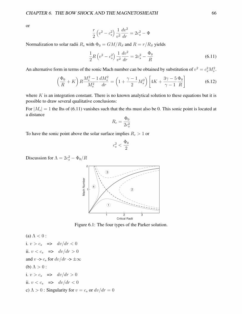
Discussion for Λ = 2c2s − Φ0/R
Mach N
um
ber
Critical Radii
1
2
1 2 3
4
3
2
1
Figure 6.1: The four types of the Parker solution.
(a) Λ < 0 :
i. v > cs => dv/dr < 0
ii. v < cs => dv/dr > 0
and v -> cs for dv/dr -> ±∞(b) Λ > 0 :
i. v > cs => dv/dr > 0
ii. v < cs => dv/dr < 0
c) Λ > 0 : Singularity for v = cs or dv/dr = 0
CHAPTER 6. THE BOW SHOCK AND THE MAGNETOSHEATH 67
Properties of the Solar Wind
Typical velocities of the solar wind range between 300 km/s and 1400 km/s with a typical value ofabout 500 km/s. Source region of the solar wind are the so-called coronal holes, which are regionwhere the magnetic field of the sun stretches out into interplanetary space, i.e., is not closed in a loopback to the sun. In the solar corona the temperature is about 1.6·106 K and density about 5·1017 cm−3.
• Velocities of the solar wind: between 300 km/s and 1400 km/s with a typical value of about500 km/s.
• Density: decreases from about 104cm−3 at 0.1 AU to about 5cm−3 at 1 AU.
• Temperature: decreases from about 106 K at 0.1 AU to about 105 K at 1 AU corresponding toapproximately 10 eV
• Thermal electron velocity ≈ 1500 km/s and thermal ion velocity 35 km/s
• Magnetic field: about 5 nT
• Alfvén speed: vA = Bsw/√µ0min ≈ 40 km/s
• Fast mode speed: cf =√
(B2 + γp) /µ0min ≈ 60 km/s
• Plasma β > 1 often
radially expanding plasma
Rotating Sun
SectorBoundary
B
Earth
Figure 6.2: Illustration of spiral and sector structure of the solar wind.
Thus the solar wind is much faster than the sound, Alfvén, and fast mode wave speeds in the frameof the Earths. This implies the existence of a shock in front of the magnetosphere - the bow shock -across which the solar wind plasma is decelerated to ‘sub-fast’ velocities which then interact with theEarth. Caused by the sun’s rotation the magnetic field has a spiral shape (Parker spiral configuration)and is usually closely aligned with the ecliptic plane.
CHAPTER 6. THE BOW SHOCK AND THE MAGNETOSHEATH 68
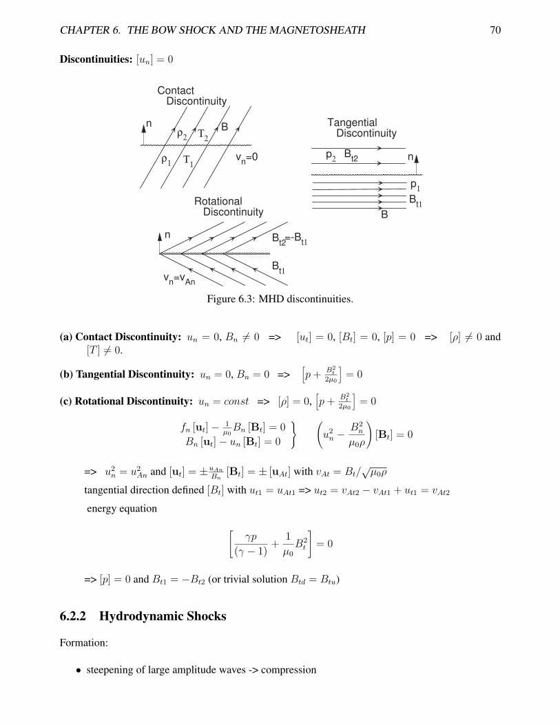
6.2 MHD Discontinuities and Shocks
The typical solar wind is much faster than the fastest MHD mode speed cf =√
(B2 + γp) /µ0min.Similar to supersonic flow past an aircraft the solar wind develops a shock in front of the magneto-sphere across which the solar wind is decelerated to velocities below the fast mode speed. In a fluidapproximation this shock can be represented as a discontinuity across which mass, momentum, andenergy has to be conserved. The jump conditions on large (fluid) scales can be derived from the MHDequations.
6.2.1 Rankine Hugoniot Conditions and MHD Discontinuities
To derive the jump conditions across a fluid boundary it is assumed that this boundary is infinitesi-mally thin and that the system is in a stationary state. The assumption of zero width is equivalent toassuming a one-dimensional boundary. Assuming a property which is conserved
∂f
∂t= −∇ · fu (6.13)
these assumption imply fun = const where un is the velocity normal to the discontinuity. Anotherway to express this result is
[fun] ≡ fdund − fuunu = 0 (6.14)
where the indexes d and u indicate the downstream and upstream regions. It is easy to show that[ab] = 1
2〈a〉 [b] + 1
2[a] 〈b〉 where In other words the flux of f is constant across the thin boundary.
To apply this method it is convenient to write the basic equation (the set of MHD equations) in aconservative form. This is already the case for the continuity equations. The momentum equation caneasily be brought into conservative form and similarly the total energy density (thermal, bulk flow,and magnetic energy) can be expressed in conservative from (implying energy conservation. Thecomplete set of equations which need to be solved are
∂ρ
∂t= −∇ · ρu (6.15)
∂ρu
∂t= −∇ ·
[ρuu +
(p+
B2
2µ0
)1− 1
µ0
BB
](6.16)
∂wtot∂t
= −∇ ·[(
1
2ρu2 +
γp
γ − 1+
1
µ0
B2
)u− u ·B
µ0
B− η
µ0
j×B
](6.17)
∂B
∂t= ∇× (u×B− ηj) (6.18)
0 = ∇ ·B (6.19)
with the total energy density
wtot =1
2ρu2 +
p
γ − 1+
1
2µ0
B2 (6.20)
Exercise: Derive the conservative form of the momentum equation.
Exercise: Derive the conservative form of the total energy density equation.
CHAPTER 6. THE BOW SHOCK AND THE MAGNETOSHEATH 69
Exercise: Why is the electric field energy not considered in the energy equation. ∇·B = 0 is usuallyan initial condition. Why is it included in the set of equation to derive the jump conditions.
Using the above set of MHD equations any steady state has to satisfy
∇ · ρu = 0 (6.21)
∇ ·[ρuu +
(p+
B2
2µ0
)1− 1
µ0
BB
]= 0 (6.22)
∇ ·[(
1
2ρu2 +
γp
γ − 1+
1
µ0
B2
)u− u ·B
µ0
B− η
µ0
j×B
]= 0 (6.23)
∇× (u×B− ηj) = 0 (6.24)∇ ·B = 0 (6.25)
To obtain the so-called Rankine Hugoniot conditions We now assume a one-dimensional boundarywith zero width and assume ideal MHD (η = 0):
n · [ρu] = 0 (6.26)
n · [ρuu] + n
[p+
B2
2µ0
]− 1
µ0
n · [BB] = 0 (6.27)
n ·[(
1
2u2 +
γp
(γ − 1) ρ+
1
µ0ρB2
)ρu
]− 1
µ0
n · [(u ·B) B] = 0 (6.28)
n× [u×B] = 0 (6.29)n · [B] = 0 (6.30)
Properties:
• Variables: ρ, u, p, B; No variables: 8; No of equations 8
• steepening of large amplitude waves -> compression
CHAPTER 6. THE BOW SHOCK AND THE MAGNETOSHEATH 71
t=t1
t=t2
cs>cs0
cs0
x
p
x
p
Figure 6.4: Illustration of wave steepening.
• fast motion of an obstacle in a gas or liquid (e.g., aircraft, space shuttle, low altitude satellites)
• waves propagating into a rarefied medium
Equations:
ndud = nuuu (6.35)pd +mndu
2d = pu +mnuu
2u (6.36)(
1
2mndu
2d +
γ
(γ − 1)pd
)ud =
(1
2mnuu
2u +
γ
(γ − 1)pu
)uu (6.37)
Introduce: Mach number M = u/cs with c2s = γp/mn
Relations:
ndnu
=(γ + 1)M2
u
2 + (γ − 1)M2u
(6.38)
uduu
=nund
(6.39)
pdpu
=2γM2
u − (γ − 1)
γ + 1(6.40)
Entropy (irreversibility):s = cV ln
p
ργ(6.41)
with cV = 1γ−1
kBm
= 3kB2m
such that ∆s = ∆s(Mu)
ds
dMu
=4γ (γ − 1) (M2
u − 1) cvMu [2γM2
u − (γ − 1)] [2 + (γ − 1)M2u ]
(6.42)
such that
ds
dMu
= 0 for Mu = 1
ds
dMu
> 0 for Mu > 1
Since sd = su for Mu = 1 => sd > su for Mu > 1 => Entropy must increase for shock!
Shock properties:
CHAPTER 6. THE BOW SHOCK AND THE MAGNETOSHEATH 72
• pressure and density increase
• velocity decreases
• entropy increases
• Mach number Md < 1
Strong shocks Mu � 1 with γ = 5/3:
ndnu
=γ + 1
γ − 1= 4 (6.43)
uduu
=γ − 1
γ + 1=
1
4(6.44)
pdpu
=2γM2
u
γ + 1(6.45)
M2d =
γ − 1
2γ=
1
5(6.46)
6.2.3 MHD Shocks
Coplanarity:
[un] 6= 0, and Bn 6= 0 =>B2n
µ0f[Bt] = [unBt]
Assume Btu = Btuey such that the z component becomes
− B2n
µ0fBzd = −undBzd (6.47)
with the solution und = B2n
µ0for Bzd = 0. Since in general und 6= B2
n
µ0f(except for Alfvén waves) the
general solution implies that the tangential fields on the two sides of the shock are aligned
Btu ‖ Btd. (6.48)
It follows that [ut] ‖ [Bt]. Thus a Galilei transformation can always render the velocities parallel tothe magnetic fields.
Basic Equations for MHD Shocks:
Assumptions: Bt = Byey, ut = uyey, and x in the normal n direction.
ρdund = ρuunu (6.49)
pd +1
2µ0
B2yd + ρdu
2nd = pu +
1
2µ0
B2yu + ρuu
2nu (6.50)
CHAPTER 6. THE BOW SHOCK AND THE MAGNETOSHEATH 73
ρdunduyd −1
µ0
BnByd = ρuunuuyu −1
µ0
BnByu (6.51)
undByd − uydBn = unuByu − uyuBn (6.52)(1
2ρdu
2d +
γpd(γ − 1)
+B2d
µ0
)und
−Bn
µ0
ud ·Bd =
(1
2ρuu
2u +
γpu(γ − 1)
+B2u
µ0
)unu −
Bn
µ0
uu ·Bu (6.53)
Parallel Shock For this case the magnetic field is parallel to the shock normal. The velocity isaligned with the magnetic field and one can always transform into a frame in which uy = 0.
Exercise: Demonstrate that the parallel shock reduces to the pure hydrodynamic shock.
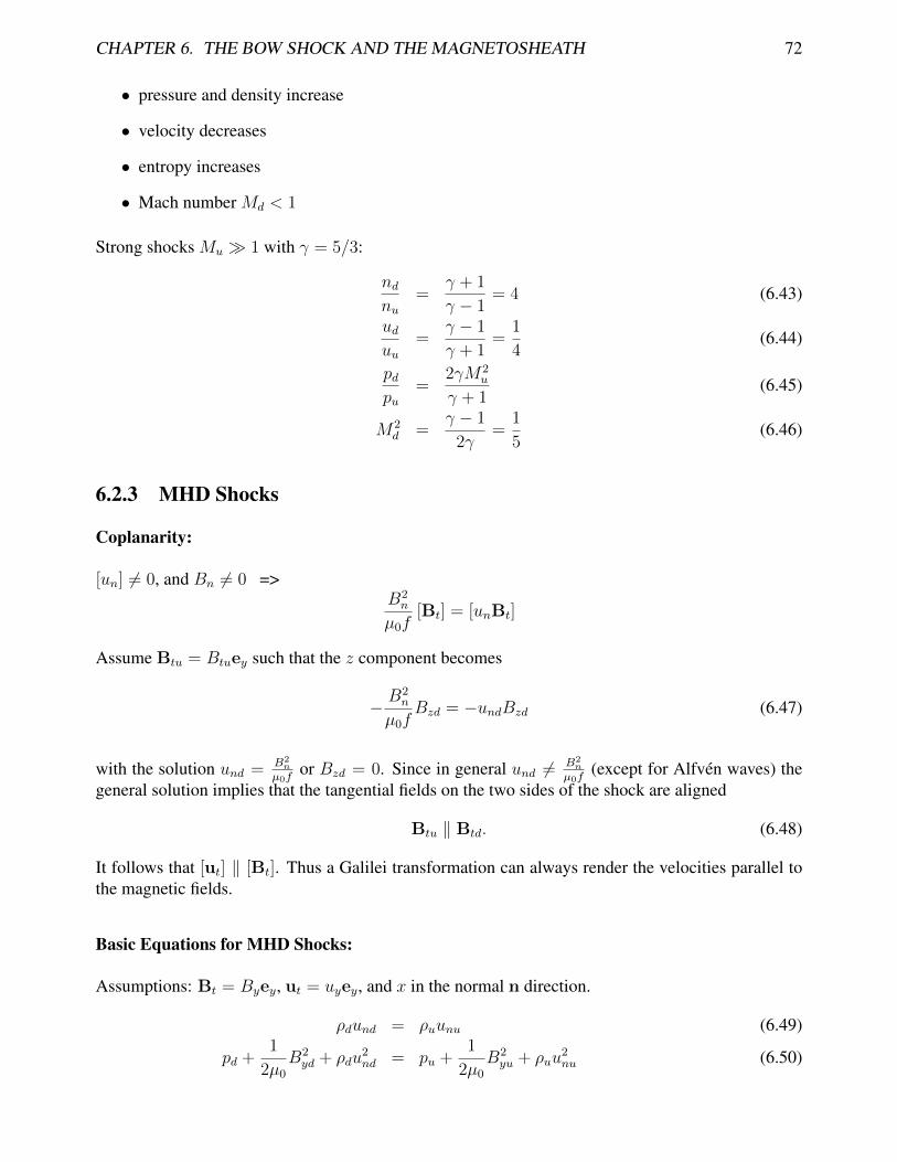
Perpendicular Shock Bn = 0. This is a special case we need to discuss because it is not containedin the general solution. Here the magnetic field is exactly perpendicular to the shock.
n
ρu
Bu
Bd
ρd p
dp
u
uu u
d uu u
d
n
Bu
Bd
ρu p
u ρdp
d
Parallel Shock Perpendicular Shock
Figure 6.5: Illustration of parallel and perpendicular shocks.
The basic equations reduce to
ρdund = ρuunu (6.54)
pd +1
2µ0
B2yd + ρdu
2nd = pu +
1
2µ0
B2yu + ρuu
2nu (6.55)
ρdunduyd = ρuunuuyu (6.56)undByd = unuByu (6.57)(
1
2ρdu
2d +
γpd(γ − 1)
+B2yd
µ0
)und =
(1
2ρuu
2u +
γpu(γ − 1)
+B2yu
µ0
)unu (6.58)
Straightforward relations:
uy = 0 (6.59)
X =ρdρu
(6.60)
undunu
=1
X(6.61)
Byd
Byu
= X (6.62)
CHAPTER 6. THE BOW SHOCK AND THE MAGNETOSHEATH 74
In addition we use
M =uucs
(6.63)
β =pthupBu
=2µ0puB2u
=2
γ
c2su2A
(6.64)
cs =
√γp
ρ(6.65)
uA =Bu√µ0ρu
(6.66)
From (6.55)
pdpu
= 1 +1
2µ0
B2yu
pu
(1−
B2yd
B2yu
)+ρuu
2nu
pu
(1− ρdu
2nd
ρuu2nu
)= 1 + β−1
(1−X2
)+ γM2
(1−X−1
)and from (6.58)
pdpu
=unuund
+γ − 1
2γ
ρuu2u
pu
(unuund− ρdu
2nd
ρuu2nu
)+γ − 1
γ
B2yu
µ0pu
(unuund−B2yd
B2yu
)
= X +γ − 1
2M2
(X −X−1
)+γ − 1
γ
2
β
(X −X2
)Equating the two expressions for pd/pu and multiplying with X and dividing by X − 1
X +γ − 1
2M2 (X + 1)− γ − 1
γ
2
βX2 + β−1X (1 +X)− γM2 = 0
Rearranging this expression X is the positive root of
f(X) = 2 (2− γ)X2 +[2β + (γ − 1) βM2 + 2
]γX − γ (γ + 1) βM2 = 0 (6.67)
Note: Only one positive root!
X
f(X)
1
Figure 6.6: f(X) for the shock equation.
(i) Shock must be compressive, i.e., X ≥ 1 implies f(1) < 0.
Using a frame of reference with Ez = −uxBy + uyBx = 0 such that
uy = unBy
Bn
(6.73)
Substitution in (6.49) - (6.53) with und = unu/X , X = ρd/ρu, u2And = u2Anu/X , and uAn = uAnuyields (
ρdu2nd −
1
µ0
B2n
)Byd =
(ρuu
2nu −
1
µ0
B2n
)Byu
orByd
Byu
=u2nu − u2Anu2nd − u2And
ρuρd
=u2nu − u2An
u2nu −Xu2AnuX
Byd
Byu
=u2u − u2Au2u −Xu2A
X (6.74)
The last result uses the property that the magnetic field and velocity are parallel (i.e., un/u = Bn/B,and the same for uAn). This also implies from Ohm’s law uy/ (Byun) = 1/Bn = const
uyduyu
=Byd
Byu
undunu
=u2u − u2Au2u −Xu2A
(6.75)
CHAPTER 6. THE BOW SHOCK AND THE MAGNETOSHEATH 76
The last two terms in the energy equation(B2yd +B2
n
µ0
)und −
Bn
µ0
ud ·Bd =
(B2yd +B2
n
µ0
)und −
Bn
µ0
(und
B2yd
Bn
+ undBn
)= 0
Such that
pd +1
2µ0
B2yd + ρdu
2nd = pu +
1
2µ0
B2yu + ρuu
2nu (6.76)(
1
2ρdu
2d +
γpd(γ − 1)
)und =
(1
2ρuu
2u +
γpu(γ − 1)
)unu (6.77)
remain to be solved. The energy equation yields
pdpu
= −γ − 1
2γ
ρdu2d
pu+unuund
(1 +
γ − 1
2γ
ρuu2u
pu
)
= −γ − 1
2
ρdu2d
ρuc2su+X
(1 +
γ − 1
2
u2uc2su
)
= X +γ − 1
2
Xu2uc2su
(1− u2d
u2u
)
Finally
pd +1
2µ0
B2yd + ρdu
2nd = pu +
1
2µ0
B2yu + ρuu
2nu
pdpu
= 1 + γu2nuc2su
(1− ρdu
2nd
ρuu2nu
)+
1
βu
(1−
B2yd
B2yu
)
= 1 + γM2u
(1−X−1
)+
1
βu
1−X2
(u2u − u2Au2u −Xu2A
)2
Combining the pressure equations yields
X
[1 +
γ − 1
2
1
c2su
(u2u − u2d
)]= 1 + γM2
u
(1−X−1
)+
1
βu
1−X2
(u2u − u2Au2u −Xu2A
)2
with u2yd from (6.75).
Introducing the angle θ between the incident magnetic field and the shock normal n, X is the solutionof (
u2u −Xu2A)2 [
Xc2s +1
2u2u cos2 θ {X (γ − 1)− (γ + 1)}
]+
1
2u2Au
2uX sin2 θ
[(γ +X (2− γ))u2u −Xu2A ((γ + 1)−X (γ − 1))
]= 0 (6.78)
CHAPTER 6. THE BOW SHOCK AND THE MAGNETOSHEATH 77
Relations:
ρdρu
= X (6.79)
undunu
=1
X(6.80)
uyduyu
=u2u − u2Auu2u −Xu2Au
(6.81)
Byd
Byu
=u2u − u2Auu2u −Xu2Au
X (6.82)
pdpu
= X +γ − 1
2
Xu2uc2su
(1− u2d
u2u
)(6.83)
Properties:
• (6.78) has 3 solutions
• Intermediate (Alfvén) wave for X = 1 and u2u = u2Au
• X ≈ 1 slow and intermediate waves => shocks for X > 1
n
Bu
Bd
uu
ud
Slow Shock
θn
Bu
Bd
ud
Fast Shock
θ
uu
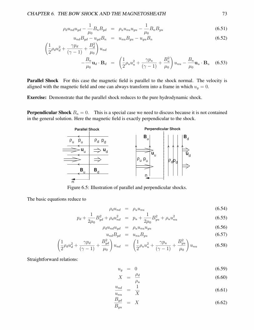
Figure 6.7: Illustration of slow and fast shocks.
Slow and fast shocks:
• Compressive with X > 1 => pd > pu
• Sign of By conserved for
– u2u ≤ u2Au => Byd < Byu and uyd < uyu - slow shock
– u2u ≥ Xu2Au => Byd > Byu and uyd > uyu - fast shock
• limit Bn -> 0
– fast: Byd/Byu -> X perpendicular shock
– slow: -> TD
CHAPTER 6. THE BOW SHOCK AND THE MAGNETOSHEATH 78
Two special cases of slow and fast shocks are switch-on and switch-off shocks
(a) Switch-off (slow) shockuu = uAu (6.84)
() => Byd = 0 tangential magnetic field is switched off!
Since uu ‖ Bu it follows that
unu =Bnu√µ0ρu
= uAn (6.85)
=> switch-off shock propagates at Alfvén speed. With the above relations the shock equationbecomes
(1−X)2[Xc2su2A
+1
2cos2 θ {X (γ − 1)− (γ + 1)}
]
+1
2X sin2 θ
[γ +X (2− γ)−X (γ + 1) +X2 (γ − 1)
]= 0
One can factorize this expression by noting that X = 1 is a solution
(1−X)2[Xc2su2A
+1
2cos2 θ {X (γ − 1)− (γ + 1)}
]
+1
2X sin2 θ ((X − 1) (γX −X − γ)) = 0
or
(X − 1)
[2X
c2su2A
+ cos2 θ {X (γ − 1)− (γ + 1)}]
+X sin2 θ ((γ − 1)X − γ) = 0
Re-arranging yields the equation which has one positive solution(2c2su2A
+ γ − 1
)X2 −
(2c2su2A
+ γ(1 + cos2 θ
))X + (γ + 1) cos2 θ = 0 (6.86)
Properties:
i. c2s/u2A > 1/2:
X ∈[1, 1 + (2c2s/u
2A + γ − 1)
−1] (X increases) for θ ∈ [0, π/2]
ii. c2s/u2A < 1/2:
X ∈[(γ + 1) / (2c2s/u
2A + γ − 1) , 1 + (2c2s/u
2A + γ − 1)
−1] (X decreases) for θ ∈ [0, π/2]
Switch-on (fast) Shock
For propagation along the magnetic field we assume
Byu = 0 (6.87)θ = 0 (6.88)
CHAPTER 6. THE BOW SHOCK AND THE MAGNETOSHEATH 79
n
Bu
Bd
uu
ud
θ = 0
Switch-on ShockSwitch-off Shock
n
Bu
Bd
uu
ud
θ
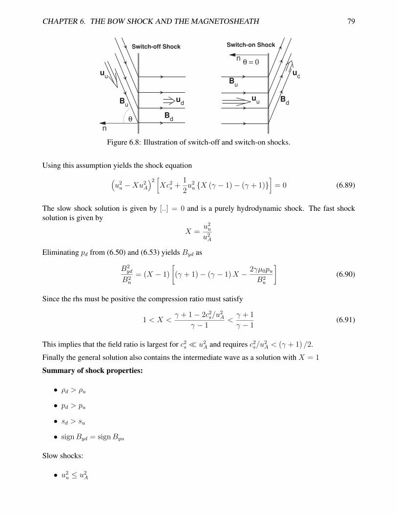
Figure 6.8: Illustration of switch-off and switch-on shocks.
Using this assumption yields the shock equation
(u2u −Xu2A
)2 [Xc2s +
1
2u2u {X (γ − 1)− (γ + 1)}
]= 0 (6.89)
The slow shock solution is given by [..] = 0 and is a purely hydrodynamic shock. The fast shocksolution is given by
X =u2uu2A
Eliminating pd from (6.50) and (6.53) yields Byd as
B2yd
B2n
= (X − 1)
[(γ + 1)− (γ − 1)X − 2γµ0pu
B2u
](6.90)
Since the rhs must be positive the compression ratio must satisfy
1 < X <γ + 1− 2c2s/u
2A
γ − 1<γ + 1
γ − 1(6.91)
This implies that the field ratio is largest for c2s � u2A and requires c2s/u2A < (γ + 1) /2.
Finally the general solution also contains the intermediate wave as a solution with X = 1
Summary of shock properties:
• ρd > ρu
• pd > pu
• sd > su
• signByd = signByu
Slow shocks:
• u2u ≤ u2A
CHAPTER 6. THE BOW SHOCK AND THE MAGNETOSHEATH 80
• Byd < Byu
• Bd < Bu
• uyd < uyu
• special case: switch-off shock
– unu = ±uAn– Byd = 0
– Strongest compression for c2s/u2A � 1, maximum X = 4
Fast Shocks
• u2u ≥ Xu2A
• Byd > Byu
• Bd > Bu
• uyd > uyu
• compression increases with Mach number
– special case: switch-on shock
– Byd = 0
– Strongest compression for c2s/u2A � 1, maximum X = 4
6.3 Properties of the Bow Shock and the Magnetosheath
6.3.1 Foreshocks and deHoffmann-Teller Frame
With the MHD plasma approximation one can analyze basic shock structure and determine down-stream conditions as a function of the upstream solar wind properties. We have argued that the reasonfor the formation of the bow shock is the super fast solar wind speed and that no information cantravel upstream from a fast shock. However, considering a kinetic plasma this is not anymore true. Inparticular any Maxwellian distribution will not only contain thermal particle but also particle althoughfew which have much higher energies than implied by the thermal motion.
To study the dynamics of particles in the vicinity of a fast shock it is instructive to use the deHoffmann-Teller frame, i.e., a frame of reference in which the shock is at rest and the electric field is 0. We haveused this frame already in deriving the general shock equation.
Usually it is simple to identify the upstream velocity normal to the shock plane unu. Moving with thisvelocity the upstream electric field is 0. However, from our derivation we know that the downstreamelectric field is nonzero. To transform into the deHoffmann-Teller frame in which the upstream and
CHAPTER 6. THE BOW SHOCK AND THE MAGNETOSHEATH 81
M'sheath
SolarWind
uu
uht
u'u
θ
B
B
y
x
Magneto
pause
Bow
Shock
Electron Foreshock
Ion Foreshock
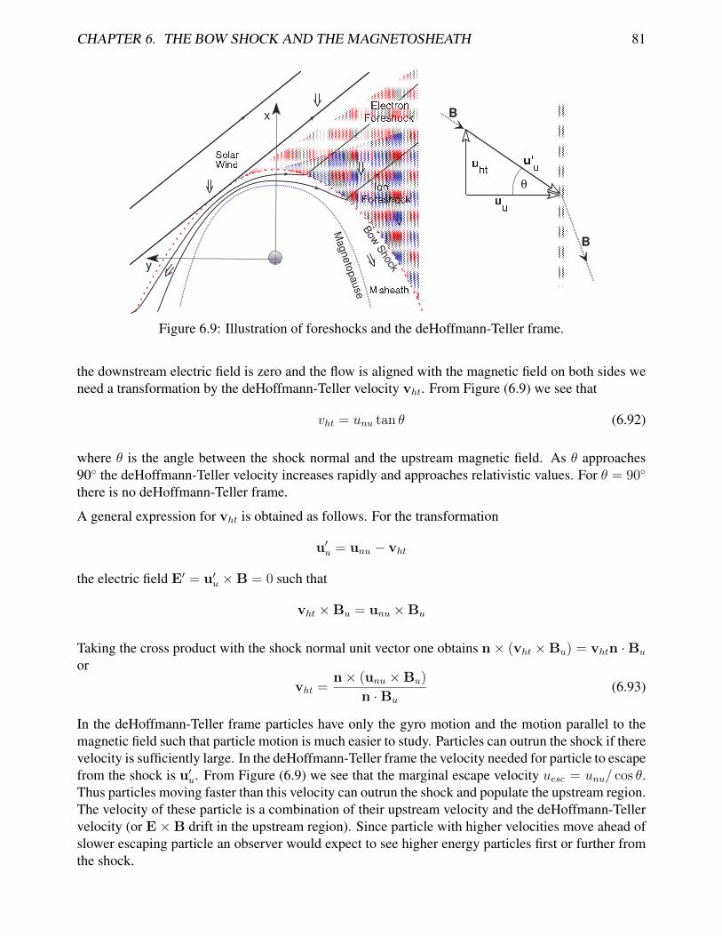
Figure 6.9: Illustration of foreshocks and the deHoffmann-Teller frame.
the downstream electric field is zero and the flow is aligned with the magnetic field on both sides weneed a transformation by the deHoffmann-Teller velocity vht. From Figure (6.9) we see that
vht = unu tan θ (6.92)
where θ is the angle between the shock normal and the upstream magnetic field. As θ approaches90◦ the deHoffmann-Teller velocity increases rapidly and approaches relativistic values. For θ = 90◦
there is no deHoffmann-Teller frame.
A general expression for vht is obtained as follows. For the transformation
u′u = unu − vht
the electric field E′ = u′u ×B = 0 such that
vht ×Bu = unu ×Bu
Taking the cross product with the shock normal unit vector one obtains n× (vht ×Bu) = vhtn ·Bu
or
vht =n× (unu ×Bu)
n ·Bu
(6.93)
In the deHoffmann-Teller frame particles have only the gyro motion and the motion parallel to themagnetic field such that particle motion is much easier to study. Particles can outrun the shock if therevelocity is sufficiently large. In the deHoffmann-Teller frame the velocity needed for particle to escapefrom the shock is u′u. From Figure (6.9) we see that the marginal escape velocity uesc = unu/ cos θ.Thus particles moving faster than this velocity can outrun the shock and populate the upstream region.The velocity of these particle is a combination of their upstream velocity and the deHoffmann-Tellervelocity (or E×B drift in the upstream region). Since particle with higher velocities move ahead ofslower escaping particle an observer would expect to see higher energy particles first or further fromthe shock.
CHAPTER 6. THE BOW SHOCK AND THE MAGNETOSHEATH 82
At the Earth the IMF is often in a Parker spiral configuration (Figure 6.2) implying that it has an angleof in the average 45◦ with the Sun-Earth line. The last field line which touches the bow shock hasa shock angle of θ = 90◦. Field lines further downstream have decreasing shock angles. Particlesoriginating from the vicinity of the first field line are the most energetic because only those can escapeup stream. The upstream region which is filled with the escaping electrons is called the electronforeshock. Ions appear to escape only if θ ≤ 70◦ such that they fill a region - the ion foreshock -downstream of the electron foreshock region.
The foreshock regions are highly turbulent. The stream of energetic particles against the incomingsolar wind is unstable with respect to many instabilities of the two-stream type. Thus the foreshockregions are rich in many different plasma waves excited by the energetic particles.
6.3.2 Shock Structure and Heating
The typical solar wind is a high-Mach number stream with Mu ≈ 8 such that the bow shock is a fastmagnetosonic shock. This also implies that density and magnetic field jump by almost a factor of 4at the subsolar (the location closest to the sun) location of the bow shock. This distance from Earthof this location is approximated by
Rbs =(
1 + 1.1nswnmsh
)Rmp (6.94)
where Rmpis the stand-off distance of the magnetopause (the location where the obstacle ‘magneto-sphere’ begins), nsw is the solar wind number density, and nmsh is the number density in the subsolarregion in the magnetosheath (downstream of the bow shock).
Away from the subsolar point the shock is curved (Figure 6.9). Because of the curvature the solarwind flow is not anymore exactly normal to the shock and the normal component of the solar windvelocity is given by
unu = nbs · usw = usw cosϕ (6.95)
where ϕ is the angle between the shock normal and the Sun-Earth line (GSM x direction). For asubsolar Mach number of 8 the Mach number is reduced to 1 for ϕ ≈ 80◦. Thus the bow shock isfinite in size limited to normal directions with ϕ < 80◦ and the shock structure changes from thesubsolar region to the periphery of the bow shock because the Mach number and the magnetic fieldand orientation relative to the shock changes.
The changing Mach number has additional implications. High-Mach number shocks are called super-critical with M > Mc and have a different structure than sub-critical M < Mc shocks. The criticalMach number is usually defined as the Mach number for which the downstream velocity is equal tothe downstream sound speed. This yields a critical Mach number ofMc ≈ 2.7. For practical purposesobservations indicate a critical Mach number < 2 for the bow shock.
The shock structure is also different for quasi-perpendicular (almost perpendicular) and quasi-parallelshocks. Particles cannot travel far into the upstream region for perpendicular shocks because the gyromotion brings them back into the shock. Typically perpendicular shocks show a shock foot where themagnetic field gradually increases in front of the main shock. Behind the main ramp the shock showsan overshoot with field values slightly larger than the asymptotic downstream values.
CHAPTER 6. THE BOW SHOCK AND THE MAGNETOSHEATH 83
Quasperp
endic
ula
rQ
uasperp
ara
llel
Foot
Ramp
Overshoot
Figure 6.10: Typical magnetic shock profiles.
Quasi-parallel shocks allow a more efficient the escape of particles. Small variations of the upstreammagnetic field orientation are amplified by the shock and generate considerable turbulence. In addi-tion - as mentioned - foreshock particles contribute to turbulent fields such that both the upstream andthe downstream region show oscillations in the plasma and magnetic field properties.
Shock Currents and Ion Acceleration
A shock leads by definition to an irreversible to heating and compression of the plasma. It thereforerequires the presence of irreversible physics such as viscosity or resistivity. The plasma at the bowshock is highly collisionless but the viscous-like or resistive-like processes can occur due the interac-tions of particles with the turbulent wave fields. However, resistivity and viscosity are insufficient toexplain shock structure and typical particle properties such as preferential ion heating. For instance,resistivity would preferentially heat electron. The dissipation in (supercritical) collisionless shock islargely controlled by the actual ion dynamics.
The change in the tangential field [Bt] corresponds to a current in the bow shock
jsh =[Bt]
µ0lsh(6.96)
where lsh is the width of the shock. This current is equivalent to the increase in the tangential fieldbehind the shock. Because of the larger gyroradii ions can penetrate deep into the compressed fieldthan electrons resulting in a thin layer with an electric field pointing toward the sun. Electrons areaccelerated by this electric field into the shock while some ions are can be reflected by this electricfield. The electric field is given by
ε0Es = e (nis + nes) le
where leis the width of the electric field layer and nis and nes are ion and electron densities in thelayer. Assuming the number of reflected ions as nir the number of ions in the shock is nis = nes−nirand the electric field is
Es =enesleε0
(1− nir
nes
)(6.97)
CHAPTER 6. THE BOW SHOCK AND THE MAGNETOSHEATH 84
Bsw
Bmsh
usw
umsh
Esw
jf
je
jsh
Es
lsh
lf
le
Figure 6.11: Ion motion at a perpendicular shock.
and all ions with energies less than eΦ = eEsle will be reflected back into the solar wind. In theE × B the reflected ions are accelerated to about twice the solar wind velocity. These reflected ionscarry the current observed in the foot region. In addition, the electric field layer causes the electronsto E×B drift while the large gyro-radii for the ions preclude this drift such that the electron carry a(Hall) current in this region.
Note, however, that the interpretation of the current structure based on single particle dynamics anddrifts should be considered with care. While the basic shock structure is reasonably representedcurrent based on single particle drifts may not be the correct representation because of diamagnetic(or in general collective) effects which are not included in the single particle dynamics. For instance,the foot current as derived from the particle drift (and acceleration is opposite to the current actuallyneeded for the magnetic field increase at the foot of the shock.
6.3.3 Magnetosheath Flow and Structure
The magnetosheath structure depends strongly on the properties of the bow shock and thus on the up-stream solar wind conditions. However, the overall shock location and the flow in the magnetosheathis to lowest order relatively well determined by purely gas dynamic models. But the magnetosheath isa very turbulent medium and there are many source for the turbulent nature of the magnetosheath. Themagnetosheath is en entirely open system with a large influx of energy from the solar wind. This is thebasic cause for the presence of the turbulence in the magnetosheath. Thus the turbulence is mainly theexpression of the many ways that the plasma (at the bow shock and in the magnetosheath) dissipatesthe energy which is carried into the system by the solar wind. Various aspect of this turbulence are
• kinetic and two-fluid (electrostatic and electromagnetic ) plasma waves close to bow shockcaused downstream plasma conditions:
– Whistler
– Lower-Hybrid
– Ion-Acoustic
• Non-MHD waves in the magnetosheath.
CHAPTER 6. THE BOW SHOCK AND THE MAGNETOSHEATH 85
– Mirror mode caused by pressure anisotropy.
– Ion-cyclotron waves driven by electrical current driven.
• Large scale magnetic field fluctuations associated with switch-on (quasi-parallel) shocks.
• MHD wave generation in the bow shock by changes in the upstream solar wind conditions.
• Fast mode wave bouncing between the bow shock and the magnetopause.
M'sheath
SolarWind
X
ZBowshock
SolarWind
X
Z
Bowshock
M'sheath
Quasi-Perpendicular Shock Quasi-Parallel Shock
Figure 6.12: Illustration of quasi-perpendicular and quasi-parallel bow shock situations.
Quasi-Perpendicular Shock
A largely perpendicular shock leads to a more pronounced pressure anisotropy with larger perpendic-ular pressure. The pressure anisotropy can be further enhanced as plasma travels from the bow shocktoward the magnetopause because field aligned flow cools the parallel pressure component This hasparticular importance for the presence of mirror waves in the magnetosheath.
Firehose and Mirror Waves: Low frequency ω � ωgi and long wavelength krgi � 1 limit kineticwaves. Without bulk motion the tensor component εs2 = 0 and with k = k‖e‖ + k⊥e⊥ the dispersionrelation splits into
k2‖c2
ω2− εs1 = 0(
k2‖c2
ω2+k2⊥c
2
ω2
)−(εs1 − εs0 +
ε2s5εs3
)= 0
The first term reduces to
ω2 = k2‖v2A
[1− 1
2
∑s
(βs‖ − βs⊥
)]
CHAPTER 6. THE BOW SHOCK AND THE MAGNETOSHEATH 86
This is the kinetic dispersion relation for the so-called fire hose instability. The instability operateswhen the rhs becomes negative ∑
s
(βs‖ − βs⊥
)> 2
Assuming εs3 � 1 in the low frequency limit the dispersion relation becomes(k2‖c
2
ω2+k2⊥c
2
ω2
)− (εs1 − εs0) = 0
or with ζs = ω/kvths‖ the dielectric yy component is
εyy =∑ω
2ps
ω2gs
−k2‖c
2
2ω2
βs⊥ − βs‖ + βs⊥k2⊥k2‖
(2 +
βs⊥βs‖
Z ′(ζs)
)In the very low frequency limit and small phase velocities, ω/kvthi ∼ ω/kvA � 1 one can expandthe plasma dispersion function for large arguments which yields
i(π
2
)β2i⊥βi‖
ω
kvths‖= 1 +
∑s
(βs⊥ −
β2s⊥βs‖
)+k2‖k2⊥
[1 +
1
2
∑s
(βs⊥ − βs‖
)]
B
δV||
Satellite
Path
|B|
n
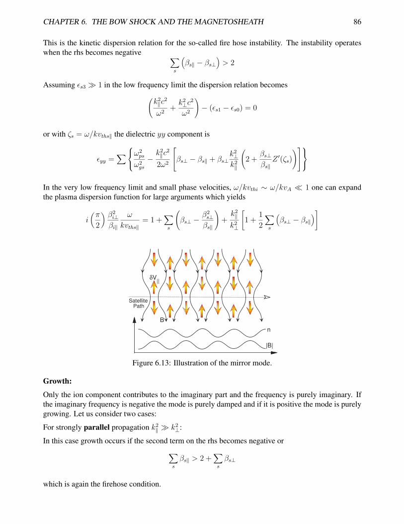
Figure 6.13: Illustration of the mirror mode.
Growth:
Only the ion component contributes to the imaginary part and the frequency is purely imaginary. Ifthe imaginary frequency is negative the mode is purely damped and if it is positive the mode is purelygrowing. Let us consider two cases:
For strongly parallel propagation k2‖ � k2⊥:
In this case growth occurs if the second term on the rhs becomes negative or∑s
βs‖ > 2 +∑s
βs⊥
which is again the firehose condition.
CHAPTER 6. THE BOW SHOCK AND THE MAGNETOSHEATH 87
For strongly perpendicular propagation k2‖ � k2⊥:
Growth occurs for ∑s
β2s⊥βs‖
> 1 +∑s
βs⊥
and the growth rate is
γm =
√2
π
βi‖β2i⊥
[∑s
βs⊥
(βs⊥βs‖− 1
)− 1
]kvthi‖
• Electrons and ion anisotropy contribute equally to instability
• Growth rate is proportional to ion thermal speed.
• Growth is favored for higher plasma beta βs = 2µ0psB2u
= 2γc2su2A
Ion-Cyclotron Waves
Dielectric function for electrostatic plasma waves for propagation with a component parallel to themagnetic field:
ε(ω k) = 1−∑s
∞∑l=−∞
ω2psΛl(ηs)
k2v2ths
[Z ′(ζs.l)−
2lωgsk‖vths
Z(ζs.l)
]
with
ζi.l =ω − lωgik‖vthi
ζe.l =ω − lωge − k‖vd
k‖vthe
Here a uniform plasma drift vd parallel to the magnetic field is assumed for the electron. For purelyparallel propagation the dispersion relation also contains ion acoustic wave for Te � Ti. For ioncyclotron waves we assume k‖ � k⊥and Te ≈ Ti with the solution
ω ≈ ωgi
[1 +
Λ1(ηi)
1 + Ti/Te −G
]
with G = Λ1 + (1− Λ0) /ηi, and ηe � 1, ζe.l � 1 and ζi.l � 1 are used. Since Λ1(ηi) < 1, andG < 1 the correction term is usually smaller than 0.5 such that the frequency is close to the ion gyrofrequency. In the limit ηi -> 0 the frequency is
ω ≈ ωgi(1 + k2⊥c
2ia/2ω2gi
)= ωgi (1 + ∆)
with c2ia = kBTe/mi
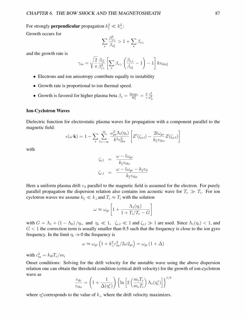
Onset conditions: Solving for the drift velocity for the unstable wave using the above dispersionrelation one can obtain the threshold condition (critical drift velocity) for the growth of ion-cyclotronwave as
vdcvthi
=
(1 +
1
∆(η∗i )
){ln[2(miTemeTi
)Λ1(η
∗i )]}1/2
where η∗i corresponds to the value of k⊥ where the drift velocity maximizes.
CHAPTER 6. THE BOW SHOCK AND THE MAGNETOSHEATH 88
0.1
vdc/v
the
Te/Ti
1.0
1 10
Unstable
Stable
l=1
l=2
Figure 6.14: Stability of ion-cyclotron waves.
Quasi-parallel shock
We know already that a quasi-parallel shock generates more turbulence both in the upstream and inthe down stream region. The shock for θ ≈ 0 is a switch-on fast shock. Therefore the downstreammagnetic field direction can vary strongly and depends on the history of the plasma and on the smallchanges in the upstream magnetic field orientation. Thus upstream changes are extremely amplifiedand small changes can entirely change the magnetosheath magnetic field.
Northward versus southward IMF
Switching the IMF from a northward to a southward direction should not have any influence on themagnetosheath flow and structure if this structure is entirely controlled by the bow shock. Albeitthe magnetosheath structure is different for north- and southward fields. A characteristic propertyof a northward IMF is a region of depleted density and thermal pressure in front of the subsolarmagnetopause. This region is absent during periods of strongly southward IMF.
B
V
V
MagnetosphereB
V
V
Streamlines
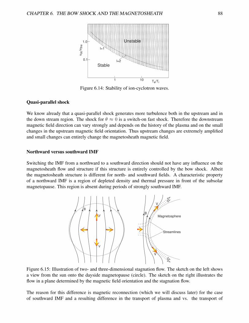
Figure 6.15: Illustration of two- and three-dimensional stagnation flow. The sketch on the left showsa view from the sun onto the dayside magnetopause (circle). The sketch on the right illustrates theflow in a plane determined by the magnetic field orientation and the stagnation flow.
The reason for this difference is magnetic reconnection (which we will discuss later) for the caseof southward IMF and a resulting difference in the transport of plasma and vs. the transport of
CHAPTER 6. THE BOW SHOCK AND THE MAGNETOSHEATH 89
magnetic flux. The magnetosheath flow and therefore the transport of plasma is three-dimensional,i.e., it occurs in the dawn and dusk directions as well as in the north and south directions as illustratedin Figure 6.15. However, the magnetic flux extends in the north-south direction and for northwardIMF it can only be removed by dawn and duskward flow. Thus plasma can be transported moreefficiently away from the subsolar region because the removing flow has an additional degree offreedom compared to the flow which can remove the magnetic field.
This may be better illustrated in two dimensions where we assume the Earth to be a cylinder and themagnetosphere a two-dimensional dipole with infinite extend in the GSM y direction. In this situationplasma can still flow around this two-dimensional magnetosphere. However, magnetic flux is stuckin front of the cylinder and cannot be removed if the IMF is northward. Thus the magnetic flux pilesup in front of this magnetosphere. For southward IMF reconnection at the dayside magnetopause candisconnect a magnetic field line and remove it from the dayside.
The fact that plasma is more easily removed along the magnetic field for northward IMF leads toan increase in the magnetic flux and magnetic field strength in front of the magnetopause. Pressurebalance then requires that the thermal pressure in this region has to decrease giving rise to the so-called plasma depletion layer.
The bow shock as a filter for solar wind perturbations
Thus far we have focused on the stationary structure of the bow shock for given solar wind conditions.However, the solar wind is a relatively unsteady medium. The typical correlation time for solar windconditions is of the order of 10 to 20 minutes, i.e, solar wind conditions typically change on thistime scale. Any perturbation present in the solar wind is transmitted through the bow shock. Theseperturbations clearly contribute significantly to the turbulent nonlinear waves in the magnetosheath.
t=t1
t=t2
p
t=t3
t=t4
-xBS MP
Figure 6.16: Illustration of fast mode bouncing between the bow shock and the magnetopause.
To illustrate the basic aspects of this wave interaction consider a one-dimensional system along theSun-Earth line. Let us assume that a fast mode rectangular wave pulse travels in the solar wind
CHAPTER 6. THE BOW SHOCK AND THE MAGNETOSHEATH 90
toward the Earth. At the bow shock this pulse cannot be reflected such that all energy, momentum,mass, and magnetic flux which is transported by the pulse must be transmitted into the downstreamregion. During the interaction the plasma condition just upstream of the shock are modified by thewave. Thus shock properties like the compression, tangential field, velocity change. In particular, alsothe deHoffmann-Teller frame will change implying that the shock location moves up- or downstreamdepending on the properties of the wave.
The downstream properties are changed because of the intermittent different shock properties. Ingeneral the perturbation created downstream cannot be represented by a single rectangular fast wave.Thus the transmitted mass, momentum, energy, and flux transport requires the presence of severalMHD waves one o which will be a now modified rectangular fast wave. The fast wave propagatesfaster downstream than Alfvén and slow waves such that it outruns the other waves. Since the fastmode wave is the only large scale fluid wave with a significant group velocity perpendicular to themagnetic field, the fast wave is the only wave that can reach the magnetopause.
At the magnetopause some of the wave energy is transmitted into the magnetosphere, however mostof it is reflected again as fast wave because of the steep density gradient at the magnetopause. Duringthe reflection/transmission other wave modes are generated to maintain mass, momentum, energy, andmagnetic flux conservation. The transmitted waves will undergo further modifications and reflectionsin the magnetosphere. The reflected fast wave is traveling back upstream through the magnetosheathto the bow shock location where it is reflected again with the side effects to move the location of thebow shock again and to generate other MHD wave. In the entire process the amplitude of the fast waveis decreasing because of coupling to other waves, transmission into the magnetosphere, transport inthe stagnation flow away from the subsolar region, and because of curvature (three-dimensionalitywhich is not considered in this simplified example.