JOURNAL OF GEOPHYSICAL RESEARCH: SPACE PHYSICS, VOL. 118, 5454–5466, doi:10.1002/jgra.50519, 2013
Magnetospheric response to magnetosheath pressure pulses:A low-pass filter effectM. O. Archer,1 T. S. Horbury,1 J. P. Eastwood,1 J. M. Weygand,2 and T. K. Yeoman3
Received 31 May 2013; revised 19 July 2013; accepted 15 August 2013; published 5 September 2013.
[1] We present observations from the magnetopause to the ground during periods oflarge amplitude, transient dynamic pressure pulses in the magnetosheath. Whileindividual magnetosheath pulses are sharp and impulsive, the magnetospheric response ismuch smoother with frequencies in the Pc5–6 range being excited in the compressionaland poloidal components of the magnetic field. We show that the magnetopause acts likea low-pass filter, suppressing timescales shorter than a few minutes. Further filteringappears to occur locally within the magnetosphere, which may be due to the unusual fieldline resonance frequency profile on this day. Ground magnetometer and radar data alongwith equivalent ionospheric currents show signatures of traveling convection vortices,similar to the response from pressure variations of solar wind origin. However, thesignatures are associated with groups of magnetosheath pulses rather than individual onesdue to the impulsive nature of the pressure variations. Thus, the scale-dependentmagnetospheric response to these transient pressure variations results in coherentsignatures on longer timescales than any individual pulse.Citation: Archer, M. O., T. S. Horbury, J. P. Eastwood, J. M. Weygand, and T. K. Yeoman (2013), Magnetospheric response tomagnetosheath pressure pulses: A low-pass filter effect, J. Geophys. Res. Space Physics, 118, 5454–5466, doi:10.1002/jgra.50519.
1. Introduction[2] Solar wind pressure variations can perturb the magne-
topause, enhance the magnetospheric field, excite direct andresonant waves (often in the Pc5 range, i.e., 2–7 mHz) in themagnetosphere, and generate traveling convection vortices(TCVs) in the ionosphere [e.g., Sibeck, 1990, and referencestherein]. Pressure variations can also originate at the bowshock and ion foreshock, e.g., hot flow anomalies (HFAs)[e.g., Burgess, 1989; Thomas et al., 1991], foreshock cavi-ties [e.g., Sibeck et al., 2002], and foreshock bubbles [Omidiet al., 2010]. These transient phenomena are also known tohave somewhat similar magnetospheric effects to those ofsolar wind origin [e.g., Sibeck et al., 2003; Hartinger et al.,2013]. In turn, Pc5 waves are believed to play a significantrole in the mass, energy, and momentum transport withinthe Earth’s magnetosphere: ULF waves accelerate auroralelectrons [e.g., Lotko et al., 1998] and are thought to playa role in mass transport [e.g., Allan et al., 1986] and the
1Blackett Laboratory, Imperial College London, London, UK.2Institute of Geophysics and Planetary Physics and Department of Earth
and Space Sciences, University of California, Los Angeles, California,USA.
3Radio and Space Plasma Physics Group, Department of Physics andAstronomy, University of Leicester, Leicester, UK.
Corresponding author: M. O. Archer, Space and Atmospheric PhysicsGroup, Blackett Laboratory, Imperial College London, Prince Consort Rd.,London SW7 2BW, UK. ([email protected])
energization and transport of radiation belt electrons [e.g.,Elkington et al., 1999].
[3] The position of the magnetopause in a steady stateis given by a balance of the solar wind dynamic pressureand the magnetic pressure at the boundary. A number ofapproaches have been used to model perturbations about thisequilibrium: Smit [1968] treated the nose of the magneto-sphere as a rigid body, Freeman et al. [1995] consideredthe magnetopause analogous to an elastic membrane, andBørve et al. [2011] approximated the boundary as a per-fectly conducting wall. All three models were linearized,resulting in damped harmonic oscillator equations of motionfor the magnetopause driven by variations in the solar winddynamic pressure. The calculated characteristic periodsranged from 2 to 12 min depending on solar wind condi-tions though were typically about 6 or 7 min, in agreementwith observed magnetopause oscillations [e.g., Andersonet al., 1968]. Freeman et al. [1995] and Børve et al. [2011]also predicted that the magnetopause motion would bestrongly damped due to the relative motion of the magne-topause and solar wind, estimating the damping ratio (thelevel of damping relative to the critical case) to be �0.41.The theoretical transmissibility (ratio of output to input) ofsuch a driven harmonic oscillator has a resonant peak of only1.63: Much lower frequencies are fully transmitted whereashigher-frequency oscillations are increasingly suppressed.Therefore, the magnetopause is thought to act somewhat likea low-pass filter to pressure variations.
[4] Inside the magnetosphere, the local characteristictimescale is given by field line resonances (FLRs), stand-ing Alfvén waves fixed at their ionospheric ends and usually
5454
ARCHER ET AL.: RESPONSE TO MAGNETOSHEATH PRESSURE PULSES
−5 0 5 10 15
−5
0
5
xGSE (RE)
y GS
E (
RE)
2008 Sep 30 (274) 12:00 − 00:00 (UT)
Figure 1. Orbits of the THEMIS and GOES spacecraftprojected in the x-y GSE plane for 30 September 2008 12:00-00:00 UT. The spacecraft positions are shown for 15:00 UT.The magnetopause (MP) and bow shock (BS) are shown(solid lines) using the Farris et al. [1991] and Peredo et al.[1995] models, respectively. The estimated orientation ofdirectional discontinuities (DD) in the solar wind on this dayis indicated by the dashed line with corresponding normal n.
described in terms of poloidal and toroidal modes [e.g.,Southwood, 1974]. Since the poloidal mode correspondsto radial motion of the plasma, implying the expansionand compression of the magnetosphere, it is necessarilycoupled to the compressional mode via density fluctuations[Kivelson et al., 1984]. However, mode conversion can alsooccur to the toroidal [e.g., Warnecke et al., 1990]. Gough andOrr [1984] modeled these transverse mode oscillations againas a damped harmonic oscillator, driven by compressionalwaves due to magnetopause disturbances. By comparisonwith observations, they suggested that a damping ratio of 0.1or greater is typical for the dayside magnetosphere. Whilstexhibiting a larger resonant peak, the suppression of higherfrequencies is expected to be greater in this case than withthe magnetopause models.
[5] Pressure variations in the magnetosheath can be usedto test these models’ predicted magnetospheric response.Glassmeier et al. [2008] showed that when the subsolarmagnetosheath pressure varies on timescales of 5–7 minwith amplitudes �0.5 nPa (�50% the ambient value) themagnetopause motion and compression/expansion of themagnetospheric field are quasi-static. However, recentlytransient pulses in the magnetosheath dynamic pressure(sometimes called jets) have been reported [e.g., Savin et al.,2008, 2011, 2012; Hietala et al., 2009, 2012; Amata et al.,2011]. These occur around 2% of the time, predominantlydownstream of the quasi-parallel shock, and have durationsof around 30 s on average and amplitudes of up to�15 timesthe ambient dynamic pressure (principally due to velocityincreases) and �2 times the ambient total pressure [Archerand Horbury, 2013]. They also tend to be quasiperiodic,recurring on timescales of a few minutes (F. Plaschke et al.,Anti-sunward high-speed jets in the subsolar magnetosheath,submitted to Annales Geophysicae, 2013).
[6] It is known that these pressure pulses or jets can haveimpacts within the magnetosphere. Shue et al. [2009] andAmata et al. [2011] showed that individual magnetosheathjets were able to distort and move the magnetopause �0.5–1.5 RE. Irregular magnetic pulsations at geostationary orbitand localized flow enhancements in the ionosphere werereported by Hietala et al. [2012] to be caused by jets understeady quasi-radial interplanetary magnetic field (IMF). The“mesoscale” ionospheric signatures shared some similari-ties with magnetic impulse events (MIEs) and TCVs, thoughthey did not appear to travel. In contrast, Dmitriev andSuvorova [2012] showed that a plasma jet due to a solarwind discontinuity resulted in a large-scale magnetopausedistortion of an expansion-compression-expansion sequencelasting �15 min, effective penetration of magnetosheathplasma inside the magnetosphere, and traveling ground mag-netometer signatures at low to middle latitudes over muchlarger spatial scales. It was unclear, however, how the dis-continuity of duration �1 min resulted in a much longertimescale in the response.
[7] Whilst it is evident that magnetosheath pressure pulsescan cause magnetopause motion, their subsequent effectsand how these relate to other magnetospheric phenomena arenot well understood. The response to quasiperiodic pulses,as opposed to isolated ones, is also unclear. In this paper wecontinue the study of Archer et al. [2012], who presentedTime History of Events and Macroscale Interactions duringSubstorms (THEMIS) [Angelopoulos, 2008] observations ofmagnetosheath pressure pulses consistent with being gener-ated by solar wind discontinuities interacting with the bowshock [Lin et al., 1996a, 1996b; Tsubouchi and Matsumoto,2005]. They showed evidence of magnetopause motionunder the action of groups of pulses as opposed to isolated,individual ones. Here we use data from the THEMIS Flux-gate Magnetometer [Auster et al., 2008] and ElectrostaticAnalyzer [McFadden et al., 2008a], magnetometers fromthe GOES spacecraft [Grubb, 1975], ground magnetometersacross North America and Greenland (THEMIS, CanadianArray for Realtime Investigations of Magnetic Activ-ity (CARISMA), Canadian Magnetic Observatory System(CANMOS), Magnetometer Array for Cusp and Cleft Stud-ies (MACCS), Geophysical Institute Magnetometer Array(GIMA), Technical University of Denmark (DTU), U.S.Geological Survey (USGS), and Solar-Terrestrial EnergyProgram (STEP)), and Super Dual Auroral Radar Network(SuperDARN) radar data [Greenwald et al., 1995; Chishamet al., 2007], which provide a comprehensive chain of obser-vations from the magnetosheath to the ground in order tostudy the pulses’ magnetospheric response.
2. Outer Magnetosphere2.1. Observations
[8] Figure 1 shows the positions of the spacecraft on30 September 2008. Between 15:01 UT and 22:47 UT, bothTHD and THE were in the magnetosheath, separated by�1 RE and observed periods of large amplitude pressurepulses in the magnetosheath, shown in Figure 2 (first panel).The pressure pulses were typically of duration 10 s to 2 minin the spacecraft frame and tended to recur on timescalesof 3–5 min; however, there were also large periods of time(of the order of an hour) when no pulses were observed at all.
5455
ARCHER ET AL.: RESPONSE TO MAGNETOSHEATH PRESSURE PULSES
HFAPulses
0
2
4
6
8M
agne
tosh
eath
Pto
t (nP
a)
UTTHD MLTTHE MLT
18 0010 3210 11
20 0011 0010 38
22 0011 3011 05
THDTHE
16 0010 0609 44
−20
−10
0
10
UTMLT
L (RE)
UTMLT
L (RE)
UTMLT
L (RE)
16 0012 13
6.9
18 0014 13
6.9
20 0016 13
6.8
22 0018 11
6.8
G10
ΔBF (
nT)
G11
ΔBF (
nT)
−20
−10
0
10
G12
ΔBF (
nT)
16 0011 11
6.8
18 0013 12
6.8
20 0015 12
6.8
22 0017 10
6.8
0
10
20
30
16 0007 07
6.7
18 0009 076.7
20 0011 076.6
22 0013 066.6
−10
0
10
20
30
UTMLT
L (RE)
16 00 18 0011 31
9.3
20 0012 18
7.7
22 0013 40
5.0
TH
AΔB
F (
nT)
ObservationsQuasistatic & 6 min smooth Predictions
Figure 2. (first panel) Magnetosheath total pressure as measured by THD (turquoise) and THE (blue).Periods of pressure pulses are indicated by magenta bars and a pressure decrease consistent with a HFA ishighlighted by the downward pointing triangle. (second to fifth panels) Changes in the mean field-alignedcomponent of the magnetic field observed by THA and the three GOES spacecraft are given by the blacklines where the predicted field magnitude from the T96 model for average upstream conditions has beensubtracted. Predicted changes in field magnitude from T96 using THD observations are shown for quasi-static (grey) and 6 min smoothed (red) magnetospheric responses. Additional horizontal axes indicate thespacecraft magnetic local time (MLT) and L-shell.
The total pressure (ion thermal + electron thermal + dynamic+ magnetic) of the pulses was 2–4 times that of the ambi-ent plasma, with the enhancements chiefly being due to 3–10times increases in the dynamic pressure. These dynamicpressure enhancements were mainly due to increases in theflow velocity [Archer et al., 2012].
[9] Magnetic field data from THA and the GOES space-craft were transformed into a mean field-aligned coordinatesystem (MFA) with the field-aligned component F (givenby a 20 min moving average) representative of compres-sional modes, the azimuthal component A = F � r (wherer is the spacecraft’s geocentric position, thus A points east)representative of toroidal Alfvénic modes, and the radialcomponent R (completing the right-handed set pointing
toward the Earth) representative of poloidal Alfvénic modes.Figure 2 shows the changes in the field-aligned compo-nent (black), where the predicted field magnitude from theT96 model [Tsyganenko, 1995; Tsyganenko and Stern, 1996]using average upstream conditions has been subtracted sothat observed fluctuations are clearer. We only show THAdata between 18:00 and 22:00 UT as a number of low-latitude boundary layer crossings were observed before then[Archer et al., 2012] and afterward the magnetic field direc-tion was changing faster than the averaging period, resultingin a poor estimate of F.
[10] Using the magnetosheath total pressure measure-ments as input to the T96 model, the predicted quasi-staticresponse of the magnetosphere to pressure variations at the
5456
ARCHER ET AL.: RESPONSE TO MAGNETOSHEATH PRESSURE PULSES
3 4 5 6 7 8 9 10
L (RE)
n (
cm)
0
1
2
3
4
5
6
f FLR
(m
Hz)
Figure 3. L-shell profiles of the magnetospheric electronnumber density observed by THA (light and dark blue, thelatter has been smoothed) and the estimated fundamentalfield line resonant frequency (black).
spacecraft locations can be found as shown in Figure 2(grey) using THD data. During intervals without pulses,the compressional variations of the magnetospheric fieldwere similar to these predictions (with some systematic dif-ferences due to the statistical nature of the T96 model),consistent with Glassmeier et al. [2008]. It is clear, how-ever, that the response to the pulses was different since theobserved compressions of �1–10 nT (similar to those ofHietala et al. [2012] and Dmitriev and Suvorova [2012])were much weaker and smoother than the sharp and impul-sive magnetosheath pressure variations.
2.2. Analysis[11] Although the magnetosheath pressure pulses con-
tained variations over a wide range of frequencies due totheir short timescales and quasiperiodicity, the harmonicoscillator models of the magnetopause [Freeman et al.,1995; Børve et al., 2011] predict a response somewhat likea low-pass filter with a typical timescale of about 6 or7 min. Therefore, we smoothed the THD magnetosheathtotal pressure measurements by a 6 min running average(THE yielded qualitatively similar results) before inputtingto the T96 model, giving more realistic predictions whichare shown in Figure 2 (red). The predicted responses tothe pulses, which could not be accounted for simply by thesolar wind pressure, show good agreement with the mag-netospheric observations overall. For the periods of pulsesbetween 18:30 and 19:05 UT, the prediction yields threecompressions of similar amplitude to those observed byTHA and G11. THA also observed some higher frequen-cies which the smoothing does not capture, e.g., the twopeaks in the 18:35 UT compression corresponding to twoindividual magnetosheath pressure pulses. These featureswere not as prominent at geostationary orbit, consistentwith further filtering occurring at progressively lower L-shells. Between 21:00 and 23:00 UT, G11 and THA (whenapplicable) observations showed further agreement with thepredictions (G10 and G12 were close to dusk during thisperiod) though underestimated the response by �0.5–1 nT.Around 17:00 UT, the agreement was less clear, though bothsignatures were small at less than �0.5 nT.
[12] The predictions made through smoothing the mag-netosheath pressure highlight the collective effect ofpulses: The magnetospheric responses occurred over longer
timescales and were due to many pulses rather than individ-ual ones. This furthers the suggestion of Hietala et al. [2012]that pulses may have cumulative effects and that a one-to-one correspondence between individual pulses and theireffects is not always clear. The filtering effect of the mag-netopause may also account for the 15 min period responsereported by Dmitriev and Suvorova [2012] due to a �1 minmagnetosheath jet associated with a discontinuity, thoughthe origin of the expansion-compression-expansion signa-ture for that event is not clear since the magnetosheathpressure was only observed during the jet.2.2.1. Time-Frequency Analysis
[13] Whilst a characteristic period of about 6 min isthought to be associated with the magnetopause, the localrelevant timescale within the magnetosphere is that of fieldline resonances (FLRs) and these were estimated using thetime of flight approximation:
fFLR =�
2Z
dsvA
�–1
(1)
where fFLR is the fundamental FLR frequency, vA is theAlfvén speed, and the integration is carried out over theentire length of the field line. Note that we make no dis-tinction between poloidal and toroidal mode FLRs in thiscalculation, though they are typically similar [Cummings etal., 1969]. The average T96 model was used along with apower law density distribution along the field line [Radoskiand Carovillano, 1966]:
� (L, r) = �0 (L)�
Lr
�m
(2)
where r is the geocentric radial distance, L is the equato-rial distance to the field line, �0 (L) is the equatorial massdensity, and the exponent m is taken to be 2 [Denton et al.,2002; Clausen et al., 2009]. Since THA traveled from themagnetopause to the inner magnetosphere close to the equa-torial plane, �0 (L) can be determined using equation (2) andthe spacecraft potential inferred density [McFadden et al.,2008b] shown in Figure 3. Unlike the standard magneto-spheric density profile which shows a sharp jump in densityat the plasmapause, the wave implications of which havebeen modeled extensively [e.g., Lee and Lysak, 1989], THAobserved a steady increase in electron density of 4 ordersof magnitude from L � 9–5 similar to that reported byTu et al. [2007] during magnetospheric quiet times. In ourcalculation, the density was smoothed using a 20 min run-ning average to remove fluctuations and the atomic masswas assumed to be 1. Assuming �0 (L) did not change sig-nificantly over this interval, the FLR frequencies were alsoestimated for the GOES spacecraft. The calculations resultedin fFLR � 0.5–6 mHz, i.e., in the Pc5–6 range, though itshould be noted that due to the density profile here, the con-figuration of the FLR frequencies is rather different to thosepreviously modeled [e.g., Lee and Lysak, 1989]. Our com-puted frequencies are consistent with those obtained by Wildet al. [2005] using a similar method which were validatedagainst numerical solutions to the wave equations as wellas observed geomagnetic pulsations. While previous studieshave shown that the difference between estimated FLR fre-quencies using different models can be large [Berube et al.,2006; McCollough et al., 2008], here it was found that using
5457
ARCHER ET AL.: RESPONSE TO MAGNETOSHEATH PRESSURE PULSES
a dipole model field changed the results by only �1 mHzat the largest L-shells and this difference rapidly becamenegligible with decreasing L-shell. Similarly, changing theexponent of the density distribution had little effect on theresults. Thus, we are confident that our estimated frequenciesare broadly correct; indeed in this study, we do not requireprecise FLR frequencies.
[14] To examine the frequency content of magneto-spheric pulsations during intervals of magnetosheath pulses,dynamic spectra of the magnetic field data in the MFA sys-tem were calculated using the Morlet wavelet transform[Torrence and Compo, 1998]. The results for the field-aligned (with the mean field subtracted) and radial com-ponents are shown in Figure 4 for THA, G10, and G11(G12 was similar to G10, an hour later in MLT) along withthe phase difference when well defined (wavelet coherence[Torrence and Webster, 1999] greater than 0.75). The esti-mated first three harmonics of FLR frequencies are shownas the black lines. Also shown is the expected frequencyof upstream ULF waves generated in the ion foreshock[Takahashi et al., 1984] which are convected into the mag-netosphere [e.g., Clausen et al., 2009]:
fUW [mHz] = 7.6B0[nT] cos2 �Bx (3)
where B0 is the IMF strength and �Bx is the IMF cone angle,calculated from 1 min smoothed (to remove contaminationfrom upstream waves) THB data. At the spacecraft loca-tions this was typically distinct from the FLR frequency.Pulsations at the upstream wave frequency are seen inFigure 4 often coincident with periods of pulses since theyoccur downstream of the quasi-parallel shock [Archer et al.,2012].
[15] Figure 4 shows that THA observed, between 18:30and 19:05 UT, large increases in the compressional modepower at the fundamental FLR frequency and below, withmuch less power at higher frequencies (apart from at theupstream wave frequency). The same interval observed bythe GOES spacecraft, whilst lower power, also showedthe largest increases at or below their respective funda-mental FLR frequencies, which were lower than those forTHA. Thus, further filtering of the compressional compo-nent occurred at lower L-shells. This may be due to theunusual FLR frequency profile on this day, which went downwith decreasing L-shell from the magnetopause to L � 6.Near the magnetopause, broadband compressional waves attimescales of �3 min and longer would be expected due tothe action of the pulses, as was observed by THA at around18:35 UT. At each L-shell, compressional power may res-onantly convert to toroidal modes, thus at a lower L-shell,there would appear to have been a filtering effect suppress-ing frequencies greater than the fundamental. It is beyond thescope of this study to discount other potential mechanismsof filtering under this unusual magnetospheric configura-tion. Future modeling and observational work could helpdistinguish between these mechanisms.
[16] During other periods of pulses, GOES observationsagain showed enhancements in the power typically at orbelow the FLR frequency. At around 21:00 UT, THAobserved enhancements in power at frequencies �3 mHzwhich, while above the local FLR frequency, were consis-tent with the characteristic timescales of the magnetopause.
Since we lack observations close to the magnetopause at thistime, it is unclear whether this response is contrary to thatreported for the earlier pulses or due to other effects.
[17] The dynamic spectra of the radial component ofthe magnetic field (indicating poloidal modes) were simi-lar to the field-aligned component, but contained slightlyless power. The coherence between the two components atPc5–6 frequencies was generally good and the radial com-ponent lagged the field-aligned one, though the phasedifference did not appear to be in perfect quadrature oreven constant. The radial component of the magnetic fieldobserved by THA between 18:30 and 19:05 UT was anti-correlated with the velocity fluctuations reported by Archeret al. [2012] (not shown here), consistent with poloidalAlfvén waves propagating parallel to the magnetic field.
[18] The azimuthal component of the magnetic fieldcontained significantly less power with some evidence oftoroidal mode FLRs (typically the first and second harmon-ics) due to magnetosheath pressure pulses with �0.2 nTamplitudes at geostationary orbit, comparable to those trig-gered by solar wind pressure pulses [Sarris et al., 2010].However, frequencies consistent with FLRs were alsoobserved during some periods without any pulses. It shouldbe noted that the magnetic perturbations associated with thefundamental toroidal mode are expected to be weak near themagnetic equator and thus difficult to observe by the space-craft in this study [Singer and Kivelson, 1979]. Standingwaves have a ˙90° phase relationship between the elec-tric and magnetic fields, however, testing this using waveletanalysis on data from THA’s Electric Field Instrument[Bonnell et al., 2008] proved inconclusive.
[19] On this day, there was a notable exception to thefiltered magnetospheric response to pressure variations. Asharp drop in the magnetosheath pressure was observed byTHC, THD, and THE at around 19:15 UT (indicated infigures by a triangle) due to a tangential discontinuity inthe solar wind which satisfied the Schwartz et al. [2000]conditions for the formation of hot flow anomalies (HFAs).While no plasma data upstream of the shock were available,the magnetosheath observations were qualitatively similarto the HFA signatures reported by Eastwood et al. [2008]exhibiting flow deflections, magnetic field enhancements,density cavities, and hot plasma. The magnetospheric space-craft observed a sharp decrease in the magnetic field dueto the HFA (Figure 2) which consisted chiefly of frequen-cies at or above the fundamental FLR (Figure 4). Furtherwork is required to understand why the magnetosphericresponse to HFAs is different to those expected purely frompressure variations.2.2.2. Transfer Function
[20] We quantify the low-pass filter response of the mag-netosphere by estimating the magnetopause pressure transferfunction during periods of pressure pulses using data fromTHD and THA between 18:30 and 19:05 UT, since theywere closest in MLT (just over an hour apart) and THAwas only �1 RE antisunward of the magnetopause. Thisgives an estimate of to what degree pressure balance atthe magnetopause holds over different timescales. Using thewavelet transforms of the magnetosheath total pressure fromTHD and the magnetosphere magnetic pressure from THA,we calculate the ratio of the square-rooted time-averagedwavelet spectra over this interval (these are comparable
5458
ARCHER ET AL.: RESPONSE TO MAGNETOSHEATH PRESSURE PULSES
10−3
10−2
10−1
10−3
10−2
10−1
10−3
10−2
10−1
10−3
10−2
10−1
Rad
ial
Pol
oida
lf (
Hz)
Pha
se D
ifff (
Hz)
UTMLT
L (RE)
16 00 18 0011 319.3
20 0012 187.7
22 0013 40
5.0
Rad
ial
Pol
oida
lf (
Hz)
Pha
se D
ifff (
Hz)
UTMLT
L (RE)
16 0012 13
6.9
18 0014 13
6.9
20 0016 136.8
22 0018 116.8
HFAPulses
02468
Mag
neto
shea
thP
(nP
a)
UTTHD MLTTHE MLT
16 0010 0609 44
18 0010 3210 11
20 0011 0010 38
22 0011 3011 05
THDTHE
10−3
10−2
10−1
10−3
10−2
10−1
10−3
10−2
10−1
10−3
10−2
10−1
10−3
10−2
10−1
Fie
ld A
ligne
dC
ompr
essi
onal
f (H
z)
UW
Fie
ld A
ligne
dC
ompr
essi
onal
f (H
z)
Fie
ld A
ligne
dC
ompr
essi
onal
f (H
z)
Pha
se D
ifff (
Hz)
UTMLT
L (RE)
16 0007 076.7
18 0009 076.7
20 0011 076.6
22 0013 06
6.6
Rad
ial
Pol
oida
lf (
Hz)
(a)
(b)
(c)
(d)
Figure 4. (a) Magnetosheath total pressure in the same format as Figure 2. (b-d) Dynamic power spectrafrom the wavelet transforms of the field-aligned and radial components of the magnetic field for THA,G10, and G11. The phase difference is also shown where grey areas indicate a wavelet coherence ofless than 0.75. Estimates of the first three harmonics of field line resonances at the spacecrafts’ locationare indicated by the black lines. The expected frequency of upstream waves is shown as the white lines.Additional horizontal axes indicate the spacecraft magnetic local time (MLT) and L-shell.
5459
ARCHER ET AL.: RESPONSE TO MAGNETOSHEATH PRESSURE PULSES
THD Ptot→THA PB
18:30−19:05 UT
FLR UW
Coh
eren
ce
f (Hz)
10−3 10−2 10−10
0.2
0.4
0.6
0.8
1 10−2
10−1
100
Tra
nsfe
r F
unct
ion
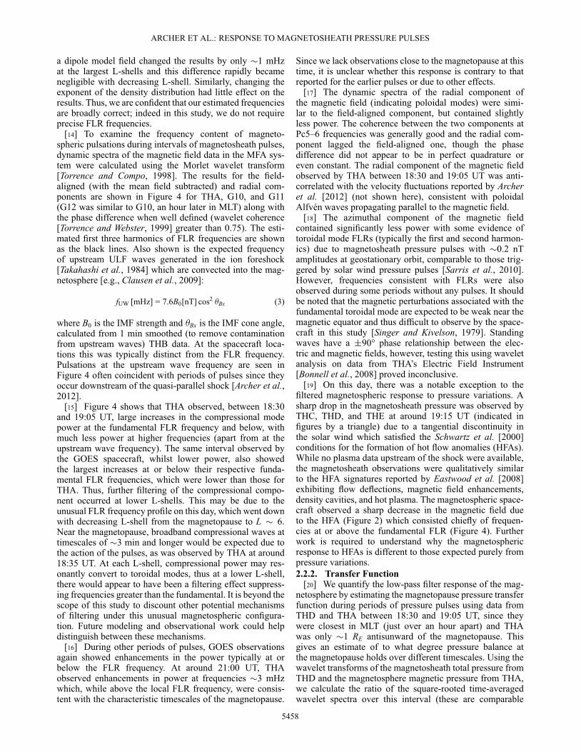
Figure 5. Estimate of the (top) magnetopause pressuretransfer function and (bottom) corresponding coherenceduring the 18:30–19:05 UT magnetosheath pulses. The reddashed lines indicate the theoretical frequency response ofa 6 min running average using the same method. Dottedblue lines indicate the range of field line resonant (FLR)frequencies over the interval used, with the light blue areaalso incorporating the spectral width of the Morlet wavelet.The magenta dotted line shows the average frequency ofupstream waves (UW) during this interval, with the lightpurple area again indicating the width of the wavelet.
to Fourier power spectral densities [Torrence and Compo,1998]). This transfer function is shown in Figure 5 (top)along with the corresponding time-averaged wavelet coher-ence (bottom), which can be interpreted as a local squaredcorrelation coefficient at a given frequency.
[21] At frequencies below the local FLR frequency, thetransfer function is large (�0.5) and the coherence is closeto unity at �0.9; hence, these frequencies are transmittedand the magnetopause reacts quasi-statically, consistent withGlassmeier et al. [2008]. At the lowest FLR frequency, thecoherence drops to �0.45 varying by only �0.05, imply-ing only some correlation between the magnetosheath andmagnetosphere. The transfer function above the range ofFLR frequencies, however, is small at �0.05. There is asmall peak corresponding to the upstream wave frequencyduring this period; however, no increase in coherence isobserved. Since upstream waves in the foreshock and mag-netosphere are quasi-monochromatic [e.g., Clausen et al.,2009] and magnetosheath pressure pulses are highly broad-band, it is unlikely that the pulses are the mechanism bywhich foreshock ULF waves propagate through the mag-netosheath. Song et al. [1993] suggested that the pressurevariations associated with compressional waves in the mag-netosheath cause the magnetopause to oscillate and reportedthat 17% of the Pc3–4 wave energy was transmitted acrossthe magnetopause. The waves in their study had a frequencyof �10 mHz, which according to our transfer function cor-responds to �5% transmission. Since our magnetosphericobservations are farther from the boundary (�1 RE), ourresults are not inconsistent with theirs.
[22] The red dashed lines in Figure 5 show the frequencyresponse and coherence of a 6 min running average. Theseare somewhat similar to the observations with some notabledifferences: At frequencies above �20 mHz, the runningaverage underestimates the transfer function and the peakin the coherence of the running average at �5 mHz is notobserved. Therefore, whilst a 6 min running average doesnot precisely capture the response of the outer magneto-sphere to the pressure variations, it nonetheless provides areasonable first approximation.
3. Ground Magnetometers3.1. Observations
[23] The times of the magnetosheath pressure pulses weresuch that many ground magnetometer (GMAG) stationsacross North America were on the dayside. Figure 6 dis-plays examples from latitudinally separated (�50° and 60°geomagnetic latitude) stations close to 12:00 MLT where theD (mean magnetic east) and H (mean magnetic north) com-ponents with the 2 h linear trend removed are shown (grey)along with 6 min smoothed data (black). Time lags (between�3 and 10 min) have been applied manually to the magne-tosheath data to align with the GMAG data since accuratelycalculating such lags is difficult.
[24] Ionospheric Hall currents rotate magnetic pulsationsby approximately 90° [Hughes and Southwood, 1976a,1976b]; hence, the D component should chiefly containpoloidal mode waves, linked to the magnetospheric com-pressions. Indeed at The Pas (TPAS), BD was very similarto the compressions observed by THA (compare withFigure 2). The lower latitude Pine Ridge (PINE) stationobserved smaller amplitudes and a much smoother response.This smoothing effect is similar to that noted when compar-ing THA observations to GOES. During the other periodsof magnetosheath pressure pulses, there was some agree-ment with the variations in the D component and thesmoothed magnetosheath pressure with some evidence ofhigher frequencies (other than the upstream wave frequency)being transmitted but suppressed, similar to the spacecraftobservations. These features were observed by all daysideGMAGs, though the amplitude of the pulsations and theirrelative frequency content varied significantly betweenstations. Variations in the H component were unlike theD component, though they were found to resemble itsnegative time derivative, e.g., at 18:35 UT TPAS observeda positive excursion in the D component and a negative-positive bipolar signature in the H component. Such arelationship is often associated with traveling convectionvortices [e.g., Glassmeier et al., 1989].
3.2. Analysis[25] To quantify the varying amplitudes of features and
their relative timings, GMAG BD observations were binnedby magnetic longitude and the time intervals containing theresponse to groups of pulses were manually identified. The2 h linear trend was removed from the time series andthe time and amplitude of the largest peak within this inter-val was then found. The results for the group of pulsesaround 18:35 UT are shown in Figure 7 (those for around18:50 UT proved similar), where the amplitudes are indi-cated by the size of the circles and their relative timings are
5460
ARCHER ET AL.: RESPONSE TO MAGNETOSHEATH PRESSURE PULSES
1
2
3
4
5
Mag
neto
shea
thP
tot (
nPa) THD
THE
BD (
nT)
BH (
nT)
UTMLT
16 3011 11
17 0011 41
17 3012 11
18 3011 24
19 0011 54
19 3012 24
21 0012 00
21 3012 30
22 0013 00
Figure 6. (top row) Magnetosheath total pressure as measured by THD (turquoise) and THE (blue). Theblack line shows the THD measurements smoothed by a 6 min running average. The applied time lagsfor the three panels are indicated and a HFA is highlighted by the downward pointing triangle. (middleand bottom rows) Stacked plots of GMAG data near the subsolar point. Grey lines show the detrended Dand H components of the field, with 6 min smoothed data shown in black. Station names, geomagneticlatitudes, and the average magnetic local time are indicated also.
given by the colors. It is clear that the signatures trackedwestward. We calculate the speed from a least squares lin-ear fit of the high-latitude data to be 9˙ 2 km s–1. Assumingevents propagate through the ionosphere and magnetospherewith a constant angular velocity [Korotova et al., 2002], thiscorresponds to a velocity of 245˙ 25 km s–1 at the magne-topause nose. The velocity along the normal of a rotationaldiscontinuity is
vn = vsw � n + vA (4)
where vsw is the solar wind velocity vector, vA is theAlfvén speed and the normal n (see Figure 1) was estimatedby the cross-product method [e.g., Knetter et al., 2004].Sibeck et al. [2003] argue pressure variations approximatelyretain their solar wind alignment in the magnetosheathsince the sum of the fast mode and convection velocitiesare of the order of the solar wind speed. Thus, we esti-mate the westward speed that the discontinuities associatedwith the group of pulses swept across the magnetopauseto be 260 km s–1 (assuming a tangential discontinuity only
Figure 7. Map of North America in geomagnetic coordinates (magnetic local time along the horizontaland geomagnetic latitude ƒ along the vertical) showing the response to the period of magnetosheathpulses at around 18:35 UT. GMAG stations are indicated by circles, where the amplitude of the observedpulsation in the D component is indicated by its size and their relative timings are given by the colors.The footprints (from the T96 model) of the spacecraft are shown as crosses and the field of view of theRankin radars is given by the green area. The GMAG stations used in Figure 6 are also highlighted.
5461
ARCHER ET AL.: RESPONSE TO MAGNETOSHEATH PRESSURE PULSES
−50
−25
0
25
50
75
j Hor
(m
A/m
)
UTMLT
18 3011 50
18 4012 00
18 5012 10
19 0012 20
19 1012 30
19 2012 40
19 3012 50
0
4
8
Mag
neto
shea
thP
tot (
nPa)
THDTHE
Figure 8. (top) Magnetosheath total pressure as measured by THD (turquoise) and THE (blue). (bottom)Feather plot of equivalent ionospheric currents at one grid point (with geomagnetic latitude 71° andthe magnetic local time indicated in the horizontal axis) as a function of time, where geomagneticnorth points upward and geomagnetic east to the right. The horizontal current magnitude is shownin red.
reduces this by �25 km s–1), consistent with the estimatefrom the ground signatures. These results are comparableto Dmitriev and Suvorova [2012] who showed low- tomiddle-latitude GMAG signatures due to a single mag-netosheath jet whose locations were consistent with thetransition in shock geometries of a solar wind discontinuityand whose relative timings were in fair agreement with thediscontinuity’s motion.
[26] The amplitude of the ground signatures increasednot only with magnetic latitude but also toward the west,e.g., at 65° geomagnetic latitude, it varied from �5 nTat 15:00 MLT to �30 nT at 07:30 MLT. This maybe because the morning sector corresponded to a morequasi-parallel bow shock and thus perhaps larger pressurevariations. Whilst such pulses are known to be most preva-lent downstream of the quasi-parallel shock [Archer andHorbury, 2013], the factors that control their amplitude areunknown. Nonetheless, it is generally known that magne-topause motions and magnetic pulsations are greater pre-noon rather than post-noon, corresponding to the location ofthe quasi-parallel bow shock under Parker spiral IMF [e.g.,Sibeck, 1990]. There are of course many other factors whichmay affect the observed amplitudes on the ground includ-ing azimuthal wave number, frequency, density distributionalong field lines, and ionospheric conductivity [e.g., Scifferand Waters, 2011].
[27] Wavelet analysis was also performed on the D andH components of the GMAG data. The results were similarto the spacecraft data in Figure 4, with enhanced Pc5–6 fre-quencies during periods of magnetosheath pressure pulses.The peaks in the spectra during the pulses, while at differ-ent powers depending on latitude and MLT, were at the samefrequencies for all stations; therefore, there was no evidenceof L-shell-dependent FLRs observed on the ground.
4. Ionosphere
4.1. Equivalent Ionospheric Currents[28] GMAG data can be used to calculate ionospheric
currents using the spherical elementary current systemmethod developed by Amm and Viljanen [1999]. Weygandet al. [2011] have applied this method to the GMAGs acrossNorth America and Greenland, finding that close to GMAGstations the derived currents were accurate to as good as 1%whereas in low coverage areas this was around 15%.
[29] An example time series of equivalent ionosphericcurrents (EICs), from the Weygand et al. [2011] database,during magnetosheath pressure pulses is shown in Figure 8,taken at 71° geomagnetic latitude and around 12:00 MLTbetween 18:30 and 19:30 UT. This grid point was only�310km away from a GMAG station; therefore, the EICs arelikely reliable. During the periods of magnetosheath pulses,there were enhancements in the horizontal currents (red).The directions of the currents showed two counterclockwiserotations between 18:30 and 19:10 UT. These signaturestracked westward like the magnetic deflections observedby the GMAGs. Assuming that ionospheric currents arecomposed mainly of Hall currents, EICs can be usedas an approximation to the plasma convection. Weygandet al. [2012] showed that in general, the EICs derivedfrom this method are antiparallel to the flows observed bythe SuperDARN radars. Therefore, the counterclockwiserotations in Figure 8 are consistent with pairs of travel-ing convection vortices (TCVs), where the vortex centerswere north of the grid point. Such pairs of vortices areexpected from transient compressions of the magnetopauseas they generate a pair of field-aligned currents which inturn have associated Hall current vortices [e.g., Sibeck et al.,2003]. The timescales of these TCV signatures were close
5462
ARCHER ET AL.: RESPONSE TO MAGNETOSHEATH PRESSURE PULSES
18 15 18 30 18 45 19 00 19 15 19 3002468
Mag
neto
shea
thP
tot (
nPa)
(a) (b) (c) (d)
Λ (°
)
18:30
MLT
(a)
06 00 08 00 10 00 12 00 14 00 16 004050607080
18:37
MLT
(b)
06 00 08 00 10 00 12 00 14 00 16 00
|jHor| mA/m
0 10 20 30 40 50Λ
(°)
18:53
MLT
(c)
08 00 10 00 12 00 14 00 16 004050607080
19:05
MLT
(d)
08 00 10 00 12 00 14 00 16 00 18 00
Figure 9. (top) Magnetosheath total pressure as measured by THD (turquoise) and THE (blue). Blackvertical lines indicate the times corresponding to subsequent panels. (a–d) Maps of North America ingeomagnetic coordinates (magnetic local time along the horizontal and geomagnetic latitude ƒ alongthe vertical). The magnitude of equivalent ionospheric currents are given by the color scale and theirdirection are shown by the arrows. Magnetometer stations used in calculating the currents are indicatedby pink squares.
to the peak of the distribution of TCVs by Clauer andPetrov [2002]. Current enhancements and signatures consis-tent with TCVs were again seen in the EICs between 21:00and 22:00 UT (not shown) which corresponded to groupsof magnetosheath pulses; however, this association was lessclear at 17:00 UT due to a following decrease in the solarwind pressure.
[30] Figure 9 shows maps of the EICs, where Figure 9a isan example of the currents without magnetosheath pressurepulses and Figures 9b–9d show the responses to three groupsof pulses. Contours of the current magnitude are shownas the colors whereas its direction is given by the arrows(which are generally smoothly varying suggesting they arereliable). The current was enhanced due to the groups ofpulses most prominently at around 70° geomagnetic latitudeand above (red areas in Figure 9). This is consistent with theoccurrence distribution of magnetic impulse events (MIEs)often associated with TCVs [e.g., Moretto et al., 2004].Note that the number of magnetometers (pink squares) atthese high latitudes is however small. The scale sizes ofthe current enhancements ranged from around 30° in mag-netic longitude up to almost the entire dayside. It is helpfulto convert timescales at the magnetopause into transversescale sizes. Since we assume the discontinuities retain theirsolar wind alignment, the responses of �3–10 min in theouter magnetosphere correspond (through multiplying bythe solar wind speed) to scale sizes along the Sun-Earth lineof �13–42 RE. Subsequently using the discontinuities’ ori-entation yields transverse scale sizes at the magnetopauseof �8–27 RE, i.e.,�30–160° magnetic longitude. Therefore,the scale sizes of the current enhancements are consistent
with the timescales on which the magnetopause responds.The vortical structure associated with TCVs is not clearfrom the EIC maps, likely because the vortex centers wereat higher latitudes than the locations of the majority ofGMAG stations.
4.2. Radar Observations[31] The Super Dual Auroral Radar Network (Super-
DARN) uses radars to measure the line-of-sight componentof the ionospheric E�B drift [Greenwald et al., 1995] and onthis day data were available from radars at Rankin and Inu-vik. Figure 10 shows data from the Rankin radars (at around10:15 MLT) in four beam directions between 16:15 and17:15 UT (see Figure 7 for the field of view). Enhancedflows were observed in a number of beam directions and inat least one beam a reversal of line-of-sight velocity. Theenhancements were typically strongest between 78 and 82°geomagnetic latitude, though coverage above this latitudewas poor. Comparing these observations with the closestGMAGs showed them to correspond to the magnetic signa-tures of the pulses shown in Figure 6. The flow structurespropagated westward (indicated by the arrow), seen from therelative timings at different beam directions (beam numberincreases toward east). Thus, SuperDARN observed a TCV(very similar to that reported by Engebretson et al. [2013])due to a group of magnetosheath pressure pulses. Whilefor other groups of pulses, further flow structures wereobserved, the data quality and coverage were often poor,and the azimuthal propagation between beam directions wasnot clear.
5463
ARCHER ET AL.: RESPONSE TO MAGNETOSHEATH PRESSURE PULSES
Bea
m 1
2Λ
(°)
Λ (°
)
75
80
85
Bea
m 9
Λ
(°)
75
80
85
Bea
m 6
75
80
85
Bea
m 3
Λ
(°)
16 15 16 30 16 45 17 00 17 1575
80
85
−800 −520 −240 40 320 600
GroundScatter
Figure 10. SuperDARN observations by the Rankin radarsfor a number of different beam directions. The color showsthe ionospheric line-of-sight velocity at different geomag-netic latitudes ƒ.
5. Discussion and Conclusions
[32] In this paper, the impact of large amplitude, tran-sient dynamic pressure pulses in the magnetosheath has beeninvestigated using observations from the magnetopause tothe ground. The pulses triggered compressional and poloidalmode waves in the outer magnetosphere typically in thePc5–6 range; such waves are important in the mass, energy,and momentum transport within Earth’s magnetosphere[e.g., Allan et al., 1986; Lotko et al., 1998; Elkington et al.,1999]. Solar wind pressure variations have similar effects[e.g., Sibeck, 1990], though these variations are generallyon comparable timescales to their responses. In contrast, themagnetosheath pulses are sharp, impulsive, and quasiperi-odic meaning they are much more broadband. Thus, themagnetopause and (under this unusual magnetospheric pro-file) lower L-shells process these variations resulting inmuch smoother responses with longer periods which are acollective effect of numerous pulses. This magnetosphericlow-pass filter suppresses frequencies much higher thanthose characteristic to the magnetopause and local field lineresonances, consistent with the suggestions of models [Smit,1968; Gough and Orr, 1984; Freeman et al., 1995; Børveet al., 2011].
[33] The GMAG networks in North America allowedsampling over a large range of geomagnetic latitudes andmagnetic local times. Signatures due to groups of pulseswere observed in the D component, which traveled westward(i.e., tailward in the morning sector) at a speed in agree-ment with the solar wind discontinuities (associated withthe pulses) sweeping across the magnetopause. The H com-ponent of the field varied like the negative time derivativeof the D component, consistent with traveling convection
vortices [e.g., Glassmeier et al., 1989]. Equivalent iono-spheric currents (EICs) also showed TCV signatures due togroups of pulses, assuming that the EICs consisted mostlyof Hall currents. In addition, SuperDARN observationsclearly showed TCV signatures due to one period of mag-netosheath pulses. Therefore, the filtered response at theouter magnetosphere to a number of magnetosheath pres-sure pulses can collectively generate a pair of TCVs inthe ionosphere. Hietala et al. [2012] presented SuperDARNdata during an interval containing many magnetosheath jets,showing localized flow enhancements which were similar toTCVs but did not appear to travel. The differences betweenthose observations and ours are likely due to the differ-ent mechanisms generating these pulses: They were notassociated with solar wind discontinuities and the authorsproposed the jets were due to ripples in the bow shock understeady quasi-radial IMF. This may explain their smaller scalesizes and why they did not travel tailward due to solarwind convection.
[34] Archer and Horbury [2013] showed that the major-ity of dynamic pressure enhancements in the magnetosheathwere not associated with discontinuities in the solar windand that the IMF was indeed steadier than usual dur-ing periods of pulses, suggesting that foreshock structuresand processes are important in their generation. Recently,Hartinger et al. [2013] showed that transient ion foreshockphenomena can be a source of Pc5 waves in the magneto-sphere. Since the response to the magnetosheath pressurepulses here was typically in the Pc5–6 range, this is sugges-tive that the signatures of transient ion foreshock phenomenain the magnetosheath may contain similar pressure pulsesthough further work is required.
[35] Finally, an interesting point is the difference in themagnetospheric response to the pressure pulses and theHFA. While models suggest that the magnetopause canonly respond to pressure variations on timescales of theorder of minutes or longer, consistent with the response tothe pulses, the impact of the HFA was on much shortertimescales, though this was in agreement to previouslyreported events [e.g., Eastwood et al., 2008; Jacobsen et al.,2009]. The reason for the different temporal responsesbetween the two transient phenomena could be addressed inthe future.
[36] Acknowledgments. This research at Imperial College Londonwas funded by STFC grant ST/I505713/1. J. P. Eastwood holds an STFCAdvanced Fellowship at Imperial College London. The work of T. K.Yeoman was supported by STFC grant ST/H002480/1. We acknowledgeNASA contract NAS5-02099 and V. Angelopoulos for use of data from theTHEMIS Mission, specifically, C. W. Carlson and J. P. McFadden for useof ESA data; J. W. Bonnell and F. S. Mozer for use of EFI data; and K. H.Glassmeier, U. Auster and W. Baumjohann for the use of FGM data pro-vided under the lead of the Technical University of Braunschweig and withfinancial support through the German Ministry for Economy and Technol-ogy and the German Center for Aviation and Space (DLR) under contract50 OC 0302. For GOES magnetometer data, we thank H. J. Singer. ForGMAG data, we thank S. Mende, C. T. Russell, I. R. Mann, D. K. Milling,M. Connors, E. Steinmetz, K. Hayashi, the CARISMA team, TromsøGeophysical Observatory, Geophysical Institute University of Alaska, theGeological Survey of Canada, and the USGS Geomagnetism Program. Theauthors acknowledge the use of SuperDARN data. SuperDARN is a collec-tion of radars funded by national scientific funding agencies of Australia,Canada, China, France, Japan, South Africa, United Kingdom, and UnitedStates of America. We also thank the reviewers for their comments.
[37] Masaki Fujimoto thanks Naiguo Lin and another reviewer for theirassistance in evaluating this paper.
5464
ARCHER ET AL.: RESPONSE TO MAGNETOSHEATH PRESSURE PULSES
ReferencesAllan, W., S. P. White, and E. M. Poulter (1986), Impulse-excited hydro-
magnetic cavity and field-line resonances in the magnetosphere, Planet.Space Sci., 34, 371–385, doi:10.1016/0032-0633(86)90144-3.
Amata, E., S. P. Savin, D. Ambrosino, Y. V. Bogdanova, M. F. Marcucci, S.Romanov, and A. Skalsky (2011), High kinetic energy density jets in theEarth’s magnetosheath: A case study, Planet. Space Sci., 59, 482–494,doi:10.1016/j.pss.2010.07.021.
Amm, O., and A. Viljanen (1999), Ionospheric disturbance mag-netic field continuation from the ground to the ionosphere usingspherical elementary current systems, Earth Planets Space, 51,431–440.
Anderson, K. A., J. H. Binsack, and D. H. Fairfield (1968), Hydromag-netic disturbances of 3- to 15-minute period on the magnetopause andtheir relation to bow shock spikes, J. Geophys. Res., 73, 2371–2386,doi:10.1029/JA073i007p02371.
Angelopoulos, V. (2008), The THEMIS mission, Space Sci. Rev., 141,5–34, doi:10.1007/s11214-008-9336-1.
Archer, M. O., and T. S. Horbury (2013), Magnetosheath dynamic pres-sure enhancements: Occurrence and typical properties, Ann. Geophys.,31, 319–331, doi:10.5194/angeo-31-319-2013.
Archer, M. O., T. S. Horbury, and J. P. Eastwood (2012), Magne-tosheath pressure pulses: Generation downstream of the bow shock fromsolar wind discontinuities, J. Geophys. Res., 117, A05228, doi:10.1029/2011JA017468.
Auster, H. U., et al. (2008), The THEMIS fluxgate magnetometer, SpaceSci. Rev., 141, 235–264, doi:10.1007/s11214-008-9365-9.
Berube, D., M. B. Moldwin, and M. Ahn (2006), Computing mag-netospheric mass density from field line resonances in a realisticmagnetic field geometry, J. Geophys. Res., 111, A08206, doi:10.1029/2005JA011450.
Bonnell, J. W., F. S. Mozer, G. T. Delory, A. J. Hull, R. E. Ergun,C. M. Cully, V. Angelopoulos, and P. R. Harvey (2008), The elec-tric field instrument (EFI) for THEMIS, Space Sci. Rev., 141, 303–341,doi:10.1007/s11214-008-9469-2.
Børve, S., H. Sato, H. L. Pécseli, and J. K. Trulsen (2011), Minute-scaleperiod oscillations of the magnetosphere, Ann. Geophys., 29, 663–671,doi:10.5194/angeo-29-663-2011.
Burgess, D. (1989), On the effect of a tangential discontinuity on ionsspecularly reflected at an oblique shock, J. Geophys. Res., 94, 472–478,doi:10.1029/JA094iA01p00472.
Chisham, G., et al. (2007), A decade of the Super Dual Auroral RadarNetwork (SuperDARN): Scientific achievements, new techniques andfuture directions, Surv. Geophys., 28, 33–109, doi:10.1007/s10712-007-9017-8.
Clauer, C. R., and V. G. Petrov (2002), A statistical investigation oftraveling convection vortices observed by the west coast Greenlandmagnetometer chain, J. Geophys. Res., 107(A7), 1148, doi:10.1029/2001JA000228.
Clausen, L. B. N., T. K. Yeoman, R. C. Fear, R. Behlke, E. A. Lucek, andM. J. Engebretson (2009), First simultaneous measurements of wavesgenerated at the bow shock in the solar wind, the magnetosphere andon the ground, Ann. Geophys., 27, 357–371, doi:10.5194/angeo-27-357-2009.
Cummings, W. D., R. J. O’Sullivan, and P. J. Coleman Jr. (1969), Stand-ing Alfvén waves in the magnetosphere, J. Geophys. Res., 74, 778–793,doi:10.1029/JA074i003p00778.
Denton, R. E., J. Goldstein, J. D. Menietti, and S. L. Young (2002), Magne-tospheric electron density model inferred from Polar plasma wave data,J. Geophys. Res., 107(A11), 1386, doi:10.1029/2001JA009136.
Dmitriev, A. V., and A. V. Suvorova (2012), Traveling magnetopausedistortion related to a large-scale magnetosheath plasma jet: THEMISand ground-based observations, J. Geophys. Res., 117, A08217,doi:10.1029/2011JA016861.
Eastwood, J. P., et al. (2008), THEMIS observations of a hot flow anomaly:Solar wind, magnetosheath, and ground-based measurements, Geophys.Res. Lett., 35, L17S03, doi:10.1029/2008GL033475.
Elkington, S. R., M. K. Hudson, and A. A. Chan (1999), Accelerationof relativistic electrons via drift-resonant interaction with toroidal-modePc5 ULF oscillations, Geophys. Res. Lett., 26, 3273, doi:10.1029/1999GL003659.
Engebretson, M. J., et al. (2013), Multi-instrument observations fromSvalbard of a traveling convection vortex, electromagnetic ion cyclotronwave burst, and proton precipitation associated with a bow shock insta-bility, J. Geophys. Res. Space Physics, 118, 2975–2997, doi:10.1002/jgra.50291.
Farris, M. H., S. M. Petrinec, and C. T. Russell (1991), The thickness of themagnetosheath: Constraints on the polytropic index, Geophys. Res. Lett.,18, 1821–1824, doi:10.1029/91GL02090.
Freeman, M. P., N. C. Freeman, and C. J. Farrugia (1995), A linear pertur-bation analysis of magnetopause motion in the Newton-Busemann limit,Ann. Geophys., 13, 907–918, doi:10.1007/s00585-995-0907-0.
Glassmeier, K. H., M. Hönisch, and J. Untiedt (1989), Ground-based and satellite observations of traveling magnetospheric convec-tion twin vortices, J. Geophys. Res., 94, 2520–2528, doi:10.1029/JA094iA03p02520.
Glassmeier, K.-H., et al. (2008), Magnetospheric quasi-static response tothe dynamic magnetosheath: A THEMIS case study, Geophys. Res. Lett.,35, L17S01, doi:10.1029/2008GL033469.
Gough, H., and D. Orr (1984), The effect of damping on geomagnetic pul-sation amplitude and phase at ground observatories, Planet. Space Sci.,32, 619–628, doi:10.1016/0032-0633(84)90112-0.
Greenwald, R. A., et al. (1995), DARN/SuperDARN: A global viewof the dynamics of high-latitude convection, Space Sci. Rev., 71,761–796.
Grubb, R. N. (1975), The SMS/GOES space environment monitor subsys-tem, NOAA technical memorandum ERL SEL 42., National Oceanic andAtmospheric Administration.
Hartinger, M. D., D. L. Turner, F. Plaschke, V. Angelopoulos, and H.Singer (2013), The role of transient ion foreshock phenomena in drivingPc5 ULF wave activity, J. Geophys. Res. Space Physics, 118, 299–312,doi:10.1029/2012JA018349.
Hietala, H., et al. (2009), Supermagnetosonic jets behind a collision-less quasiparallel shock, Phys. Rev. Lett., 103, 245,001, doi:10.1103/PhysRevLett.103.245001.
Hietala, H., et al. (2012), Supermagnetosonic subsolar magnetosheath jetsand their effects: From the solar wind to the ionospheric convection, Ann.Geophys., 30, 33–48, doi:10.5194/angeo-30-33-2012.
Hughes, W. J., and D. J. Southwood (1976a), The screening of micropul-sation signals by the atmosphere and ionosphere, J. Geophys. Res., 81,3234–3240, doi:10.1029/JA081i019p03234.
Hughes, W. J., and D. J. Southwood (1976b), An illustration of modificationof geomagnetic pulsation structure by the ionosphere, J. Geophys. Res.,81, 3241–3247, doi:10.1029/JA081i019p03234.
Jacobsen, K. S., et al. (2009), THEMIS observations of extreme magne-topause motion caused by a hot flow anomaly, J. Geophys. Res., 114,A08210, doi:10.1029/2008JA013873.
Kivelson, M., J. Etcheto, and J. G. Trotignon (1984), Global compressionaloscillations of the terrestrial magnetosphere: The evidence and a model,J. Geophys. Res., 89, 9851–9856, doi:10.1029/JA089iA11p09851.
Knetter, T., F. M. Neubauer, T. Horbury, and A. Balogh (2004), Four-pointdiscontinuity observations using Cluster magnetic field data: A statisticalsurvey, J. Geophys. Res., 109, A06102, doi:10.1029/2003JA010099.
Korotova, G. I., D. G. Sibeck, H. J. Singer, and T. J. Rosenberg (2002),Tracking transient events through geosynchronous orbit and in the high-latitude ionosphere, J. Geophys. Res., 107(A11), 1345, doi:10.1029/2002JA009477.
Lee, D.-H., and R. L. Lysak (1989), Magnetospheric ULF wave couplingin the dipole model: The impulsive excitation, J. Geophys. Res., 94,17,097–17,103, doi:10.1029/JA094iA12p17097.
Lin, Y., L. C. Lee, and M. Yan (1996a), Generation of dynamic pressurepulses downstream of the bow shock by variations in the interplan-etary magnetic field orientation, J. Geophys. Res., 101, 479–493,doi:10.1029/95JA02985.
Lin, Y., D. W. Swift, and L. C. Lee (1996b), Simulation of pressure pulsesin the bow shock and magnetosheath driven by variations in interplan-etary magnetic field direction, J. Geophys. Res., 101, 27,251–27,269,doi:10.1029/96JA02733.
Lotko, W., A. V. Streltsov, and C. W. Carlson (1998), Discrete auroralarc, electrostatic shock and suprathermal electrons powered by disper-sive, anomalously resistive field line resonance, Geophys. Res. Lett., 25,4449–4452, doi:10.1029/1998GL900200.
McCollough, J. P., J. L. Gannon, D. N. Baker, and M. Gehmeyr (2008), Astatistical comparison of commonly used external magnetic field models,Space Weather, 6, S10001, doi:10.1029/2008SW000391.
McFadden, J. P., C. W. Carlson, D. Larson, M. Ludlam, R. Abiad, B. Elliott,P. Turin, M. Marckwordt, and V. Angelopoulos (2008a), The THEMISESA plasma instrument and in-flight calibration, Space Sci. Rev., 141,277–302, doi:10.1007/s11214-008-9440-2.
McFadden, J. P., C. W. Carlson, J. Bonnell, F. Mozer, V. Angelopoulos,K. H. Glassmeier, and U. Auster (2008b), THEMIS ESA firstscience results and performance issues, Space Sci. Rev., 141, 447–508,doi:10.1007/s11214-008-9433-1.
Moretto, T., D. Sibeck, and J. F. Watermann (2004), Occurrencestatistics of magnetic impulse events, Ann. Geophys., 22, 585–602,doi:10.5194/angeo-22-585-2004.
Omidi, N., J. P. Eastwood, and D. G. Sibeck (2010), Foreshock bubblesand their global magnetospheric impacts, J. Geophys. Res., 115, A06204,doi:10.1029/2009JA014828.
5465
ARCHER ET AL.: RESPONSE TO MAGNETOSHEATH PRESSURE PULSES
Peredo, M., J. A. Slavin, E. Mazur, and S. A. Curtis (1995), Three-dimensional position and shape of the bow shock and their variationwith Alfvénic, sonic and magnetosonic Mach numbers and interplan-etary magnetic field orientation, J. Geophys. Res., 100, 7907–7916,doi:10.1029/94JA02545.
Radoski, H. R., and R. L. Carovillano (1966), Axisymmetric plasmas-phere resonances: Toroidal mode, Phys. Fluids, 9, 285, doi:10.1063/1.1761671.
Sarris, T. E., W. Liu, X. Li, K. Kabin, E. R. Talaat, R. Rankin, V.Angelopoulos, J. Bonnell, and K. H. Glassmeier (2010), THEMISobservations of the spatial extent and pressure-pulse excitation offield line resonances, Geophys. Res. Lett., 37, L15104, doi:10.1029/2010GL044125.
Savin, S., et al. (2008), High energy jets in the Earth’s magnetosheath:Implications for plasma dynamics and anomalous transport, JETP Lett.,87, 593–599, doi:10.1134/S0021364008110015.
Savin, S., et al. (2011), Anomalous interaction of a plasma flow withthe boundary layers of a geomagnetic trap, JETP Lett., 93, 754–762,doi:10.1134/S0021364011120137.
Savin, S., et al. (2012), Super fast plasma streams as drivers of tran-sient and anomalous magnetospheric dynamics, Ann. Geophys., 30, 1–7,doi:10.5194/angeo-30-1-2012.
Schwartz, S. J., G. Paschmann, N. Sckopke, T. M. Bauer, M. Dunlop,A. N. Fazakerley, and M. F. Thomsen (2000), Conditions for the forma-tion of hot flow anomalies at Earth’s bow shock, J. Geophys. Res., 105,12,639–12,650, doi:10.1029/1999JA000320.
Sciffer, M. D., and C. L. Waters (2011), Relationship between ULF wavemode mix, equatorial electric fields, and ground magnetometer data,J. Geophys. Res., 116, A06202, doi:10.1029/2010JA016307.
Shue, J.-H., J.-K. Chao, P. Song, J. P. McFadden, A. Suvorova, V.Angelopoulos, K. H. Glassmeier, and F. Plaschke (2009), Anoma-lous magnetosheath flows and distorted subsolar magnetopause forradial interplanetary magnetic fields, Geophys. Res. Lett., 36, L18112,doi:10.1029/2009GL039842.
Sibeck, D. G. (1990), A model for the transient magnetospheric responseto sudden solar wind dynamic pressure variations, J. Geophys. Res., 95,3755–3771, doi:10.1029/JA095iA04p03755.
Sibeck, D. G., T.-D. Phan, R. Lin, R. P. Lepping, and A. Szabo (2002),Wind observations of foreshock cavities: A case study, J. Geophys. Res.,107(A10), 1271, doi:10.1029/2001JA007539.
Sibeck, D. G., N. B. Trivedi, E. Zesta, R. B. Decker, H. J. Singer, A. Szabo,H. Tachihara, and J. Watermann (2003), Pressure-pulse interaction withthe magnetosphere and ionosphere, J. Geophys. Res., 108(A2), 1095,doi:10.1029/2002JA009675.
Singer, H. J., and M. G. Kivelson (1979), The latitudinal structure of Pc5 waves in space: Magnetic and electric field observations, J. Geophys.Res., 84, 7213–7222, doi:10.1029/JA084iA12p07213.
Smit, G. R. (1968), Oscillatory motion of the nose region ofthe magnetopause, J. Geophys. Res., 73, 4990–4993, doi:10.1029/JA073i015p04990.
Song, P., C. T. Russell, R. J. Strangeway, J. R. Wygant, C. A. Cattell, R. J.Fitzenreiter, and R. R. Anderson (1993), Wave properties near the sub-solar magnetopause: Pc3–4 energy coupling for northward interplanetarymagnetic field, J. Geophys. Res., 98, 187–196, doi:10.1029/92JA01534.
Southwood, D. J. (1974), Some features of field line resonances in themagnetosphere, Planet. Space Sci., 22, 483–491, doi:10.1016/0032-0633(74)90078-6.
Takahashi, K., R. L. McPherron, and T. Terasawa (1984), Dependence ofthe spectrum of Pc3–4 pulsations on the interplanetary magnetic field,J. Geophys. Res., 89, 2770–2780, doi:10.1029/JA089iA05p02770.
Thomas, V. A., D. Winske, M. F. Thomsen, and T. G. Onsager (1991),Hybrid simulation of the formation of a hot flow anomaly, J. Geophys.Res., 96, 11,625–11,632, doi:10.1029/91JA01092.
Torrence, C., and G. P. Compo (1998), A practical guide to waveletanalysis, Bull. Am. Meteorol. Soc., 79, 61–78, doi:10.1175/1520-0477(1998)079<0061:APGTWA>2.0.CO;2.
Torrence, C., and P. Webster (1999), Interdecadal changes in theENSO–Monsoon system, J. Clim., 12, 2679–2690, doi:10.1175/1520-0442(1999)012<2679:ICITEM>2.0.CO;2.
Tsubouchi, K., and H. Matsumoto (2005), Effect of upstream rotationalfield on the formation of magnetic depressions in a quasi-perpendicularshock downstream, J. Geophys. Res., 110, A04101, doi:10.1029/2004JA010818.
Tsyganenko, N. A. (1995), Modeling the Earth’s magnetospheric magneticfield confined within a realistic magnetopause, J. Geophys. Res., 100,5599–5612, doi:10.1029/94JA03193.
Tsyganenko, N. A., and D. P. Stern (1996), Modeling the global magneticfield of the large-scale Birkeland current systems, J. Geophys. Res., 101,27,187–27,198, doi:10.1029/96JA02735.
Tu, J., P. Song, B. W. Reinisch, and J. L. Green (2007), Smooth elec-tron density transition from plasmasphere to the subauroral region, J.Geophys. Res., 112, A05227, doi:10.1029/2007JA012298.
Warnecke, J., H. Lühr, and K. Takahashi (1990), Observational featuresof field line resonances excited by solar wind pressure variations on 4September 1984, Planet. Space Sci., 38, 1517–1531, doi:10.1016/0032-0633(90)90157-L.
Weygand, J. M., O. Amm, A. Viljanen, V. Angelopoulos, D. Murr,M. J. Engebretson, H. Gleisner, and I. Mann (2011), Application andvalidation of the spherical elementary currents systems technique forderiving ionospheric equivalent currents with the North American andGreenland ground magnetometer arrays, J. Geophys. Res., 116, A03305,doi:10.1029/2010JA016177.
Weygand, J. M., O. Amm, V. Angelopoulos, S. E. Milan, A. Grocott, H.Gleisner, and C. Stolle (2012), Comparison between SuperDARN flowvectors and equivalent ionospheric currents from ground magnetometerarrays, J. Geophys. Res., 117, A05325, doi:10.1029/2011JA017407.
Wild, J. A., T. K. Yeoman, and C. L. Waters (2005), Revised time of flightcalculations for high latitude geomagnetic pulsations using a realisticmagnetospheric magnetic field model, J. Geophys. Res., 110, A11206,doi:10.1029/2004JA010964.