CHAPTER 7: FUNDAMENTAL MIXING AND COMBUSTION EXPERIMENTS FOR PROPELLED HYPERSONIC FLIGHT

A. D. Cutler*, G. S. Diskin†, P. M. Danehy‡, J. P. Drummond§

8.1 NOMENCLATURE ks Thermal conductivity of wall (W/mK) ns Number of samples np Number of parameters pamb Ambient pressure pexit Nozzle exit pressure pref,CJ Center-jet nozzle reference pressure pref,coflow Coflow nozzle reference pressure Prt Turbulent Prandtl number q Heat flux (W/m2) Sct Turbulent Schmidt number t Time (s) T Temperature (K) Tamb Ambient temperature Tt,CJ Center-jet nozzle total temperature Tt,coflow Coflow nozzle total temperature u Velocity x, y, z Position coordinates αs Thermal diffusivity of wall (m2/s) χ Mole fraction center-jet gas σ Standard deviation 8.2 INTRODUCTION Computational fluid dynamics (CFD) codes are extensively employed in the design of high-speed air breathing engines. CFD analysis based on the Reynolds averaged Navier-Stokes equations uses models for the turbulent fluxes that employ many ad hoc assumptions and empirically determined coefficients. Typically, these models cannot be applied with confidence to a class of flow for which they have not been validated. Two studies have been conducted to provide data suitable for code development and testing. The first experiment1, ,2 3 is a study of a coaxial jet discharging into stagnant laboratory air, with center jet of a mixture of 5% oxygen and 95% helium by volume and coflow jet of air. The exit flow pressure of both center-jet and coflow nozzles is 1 atmosphere. The presence of oxygen in the center jet is to allow the use of an oxygen flow-tagging technique (RELIEF4) to obtain non-intrusive velocity measurements. Both jets are nominally Mach 1.8, but, because of the greater speed of sound, the center jet velocity is more than twice that of the coflow. The mixing layer which forms between the center jet and the coflow near the nozzle exit is compressible, with a calculated convective Mach number5 of ~ 0.7. This geometry has several advantages: The streamwise development of the flow is generally dominated by turbulent

_____________________________________________________

* The George Washington University, MS 335, NASA Langley Research Center, Hampton, VA 23681. † Laser & Electro-optics Branch, MS 468, NASA Langley Research Center, Hampton, VA 23681. ‡ Instrumentation Systems Development Branch, MS 236, NASA Langley Research Center, Hampton, VA 23681. § Hypersonic Airbreathing Propulsion Branch, MS 197, NASA Langley Research Center, Hampton, VA 23681.

1

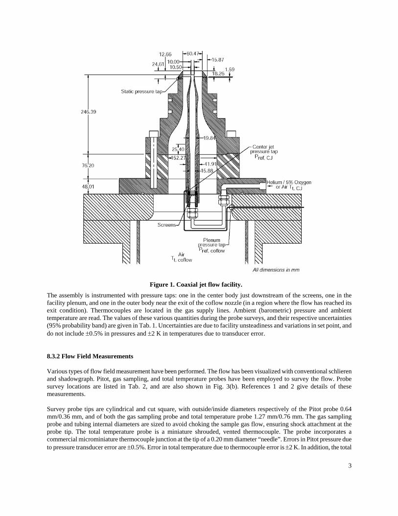
stresses (rather than pressure forces), and thus calculations are sensitive to turbulence modeling. It includes features present in supersonic combustors, including a compressible mixing layer near the nozzle exit and a light-gas/air plume downstream. Since it is a free jet, it provides easy access for both optical instrumentation and probes. Since it is axisymmetric, it requires fewer experimental measurements to fully characterize, and calculations can be performed with more modest computer resources. However, weak shock waves formed at the nozzle exit strengthen and turn normal as they approach the axis, complicating the flow. Care is thus taken in the design of the facility to provide as near as possible to 1-D flow at the exit of both center and coflow nozzles, and to minimize the strength of waves generated at the nozzle exit. Results from this experiment are compared to CFD solutions obtained by VULCAN, a previously developed code used in engine analysis.6 The second experiment7 is a study of a supersonic combustor consisting of a diverging duct with single downstream-angled wall injector. Thus, the geometry is relatively simple and large regions of subsonic recirculating flow are avoided. The nominal entrance Mach number is 2 and the enthalpy of the test gas (hot air “simulant”) is nominally that of Mach 7 flight. It was believed, on the basis of calculations performed8 that this would produce mixing-limited flow, that is to say, one for which chemical reaction to equilibrium proceeds at a much greater rate than mixing. It later proved that this was not the case. The primary experimental technique employed is coherent anti-Stokes Raman spectroscopy, known by its acronym CARS. An introduction to CARS is given by Eckbreth9, and an application of CARS to supersonic combustors is given by Smith et al.10. The species probed is molecular nitrogen and the quantity measured is temperature. Intrusive probes, such as Pitot, total temperature, hot-wire, etc., are not used due to access difficulty and high heat flux in the combustor, and because they may alter the flow. CARS has several advantages over other optical methods. It is a relatively mature and well-understood technique. Signal levels are relatively high and the signal is in the form of a coherent (laser) beam that can be collected through small windows. Incoherent (non-CARS) interferences are rejected by spatial filtering. Application of a complicated technique like CARS in high-speed engine environments is not routine. Since it is a pointwise (rather than planar) technique, building a “picture” of the internal temperature field of the combustor requires hundreds of facility runs, which is expensive. Thus, modern-design-of-experiments (MDOE) techniques are used to minimize the quantity of data required to meet the goals of this work and to minimize systematic errors associated with random errors. Details of the MDOE aspects are not discussed in this paper, but may be found in Ref. 7. 8.3 SUPERSONIC COAXIAL JET EXPERIMENT 8.3.1 Flow Facility The coaxial jet assembly is shown in Fig. 1. It is axisymmetric and consists of an outer body and a center body. The passages formed by the space between these bodies, and by the interior passage of the center body, are nozzles designed by the method of characteristics to produce 1-D flow at their exits. The nozzle assembly is joined to the Transverse Jet Facility, located in the laboratories of the Hypersonic Airbreathing Propulsion Branch at NASA Langley Research Center. The plenum of this facility contains porous plates for acoustic dampening and screens for flow conditioning. Air is provided to the facility from a central air station, and the helium-oxygen mixture is provided to the center body from a bottle trailer containing premixed gas.

pref,coflow (kPa) 580 ± 2

Tt,coflow (K) 300 ± 6 pref,CJ/pref,coflow 1.060 ± 0.008 Tt,CJ/Tt,coflow 1.02 ± 0.05 pamb/pref,coflow 0.1758 ± 0.0012 Tamb/Tt,coflow 0.982 ± 0.017 pexit/pref,coflow 0.1748 ± 0.0005

Table 1. Experimental flow parameters.

2

The assemblyfacility plenuexit conditiotemperature a(95% probabido not includ 8.3.2 Flow F Various typesand shadowgsurvey locatimeasurement Survey probemm/0.36 mmprobe and tubprobe tip. Thcommercial mto pressure tra

Figure 1. Coaxial jet flow facility.

is instrumented with pressure taps: one in the center body just downstream of the screens, one in the m, and one in the outer body near the exit of the coflow nozzle (in a region where the flow has reached its n). Thermocouples are located in the gas supply lines. Ambient (barometric) pressure and ambient re read. The values of these various quantities during the probe surveys, and their respective uncertainties lity band) are given in Tab. 1. Uncertainties are due to facility unsteadiness and variations in set point, and e ±0.5% in pressures and ±2 K in temperatures due to transducer error.

ield Measurements

of flow field measurement have been performed. The flow has been visualized with conventional schlieren raph. Pitot, gas sampling, and total temperature probes have been employed to survey the flow. Probe ons are listed in Tab. 2, and are also shown in Fig. 3(b). References 1 and 2 give details of these s.

tips are cylindrical and cut square, with outside/inside diameters respectively of the Pitot probe 0.64 , and of both the gas sampling probe and total temperature probe 1.27 mm/0.76 mm. The gas sampling ing internal diameters are sized to avoid choking the sample gas flow, ensuring shock attachment at the e total temperature probe is a miniature shrouded, vented thermocouple. The probe incorporates a icrominiature thermocouple junction at the tip of a 0.20 mm diameter “needle”. Errors in Pitot pressure due nsducer error are ±0.5%. Error in total temperature due to thermocouple error is ±2 K. In addition, the total

3

temperature probe is found to read about 1% low, due to incomplete stagnation of the flow at the sensor and/or radiation losses.

Figure 2. The RELIEF technique.

The mole fraction of the center-jet gas (i.e., the helium-oxygen mixture) in the gas withdrawn from the flow, χ, is found in real time by a hot-film probe based system11. The largest contribution to the uncertainty of the system is the manufacturer-quoted ±1% of full scale in the mass flow controller used to provide a known helium-oxygen/air mixture to calibrate the system. Maximum uncertainty in mole fraction of helium-oxygen is in the range ±1-1.5%, but uncertainty is less than this with mole fractions near 0.0 or 1.0 where there is no uncertainty in the composition of the calibration mixture.

4

The probes were mounted in a diamond-airfoil strut, and translated in the flow by a two-component stepping-motor driven translation stage. Probe “zero” location was determined using machined fixtures mounted to the nozzle exit (conical extension cap removed). Surveys were conducted across a diameter of the flow. Analysis of the data to find the best-fit center showed it to be within 0.4 mm (95% of the time) of the measured center. Thus, probe surveys are taken to pass through the axis of the jet ±0.4 mm. Survey data presented have been shifted (by less than ±0.4 mm) so that the best fit center lies at y = 0. Resulting data are found to be almost perfectly symmetrical. In addition to these “conventional” techniques, the RELIEF4 (Raman Excitation plus Laser-Induced Electronic Fluorescence) oxygen flow tagging technique, illustrated in Fig. 2, has been used to provide measurements of (instantaneous) axial component velocity. RELIEF is a time-of-flight technique which involves two steps. In the first (“tag”) step, oxygen in a line segment of the flow is excited to a non-equilibrium vibrational state by stimulated Raman scattering. This is achieved by focusing (50 cm focal length) collinear laser beams at 532nm and 580 nm. These beams are generated by passing a 200 mJ doubled Nd:YAG laser beam (532 nm) through a 6.9 MPa Raman cell containing a 50:50 mixture of helium and

oxygen. The Raman cell is seeded with light from a broadband dye laser pumped by doubled residual infrared light from

Number x, mm x, mm

RELIEF 1 0.13 2 2 3.1 5 3 10.0 12 4 17.9 17 5 27.8 27 6 42.9 42 7 61.9 62 8 81.1 82 9 100.6 102

10 121.4 123 11 150.8 153 12 181.0 190 13 220.4 220 14 261.0 258

Table 2. Experimental survey locations.

the Nd:YAG laser. The non-equilibrium oxygen returns to equilibrium only slowly as it convects with the flow. In the second “probe” step of the technique, the non-equilibrium region is found by laser-induced fluorescence imaging. This is achieved with a 20 mJ narrow band (approximately 0.5 cm-1) ArF excimer (193 nm) laser beam cylindrically focused to a 10 mm high Η 0.5 mm thick sheet in the region where the tagged flow is expected to be. The resulting fluorescence is imaged using a double intensified video-rate CCD camera, with f/4.5 UV lens and extension rings for closeup operation. Data were acquired at 5 Hz. The resulting data consist of images of displaced line pairs, acquired either at different delay times after the tag, or with one of the lines acquired prior to operation of the jet (i.e., with zero flow velocity). The instantaneous velocity is determined by finding, in subsequent data reduction, the line displacement at various points along it, and dividing by the probe delay time. A calibration is required to establish the relationship between position in the image and position in space. Mean u-component velocity and root mean square fluctuation have been obtained by this technique. Uncertainties in this data are approximately ±3% due to uncertainty in the magnification factor between flowfield and image and uncertainty in the zero point.

8.3.3 Calculation The Favre-averaged Navier-Stokes equations are solved using VULCAN, a structured, finite-volume CFD code. The calculation assumes an axisymmetric flow of a mixture of thermally perfect gases. The calculation was performed on a structured grid generated by a separate, commercial code. There are a total of 188,080 cells, distributed among five blocks. Grid points are clustered near the walls of the nozzles to resolve the boundary layers, at the exit of the center-jet nozzle to resolve the recirculation zone and shocks in the vicinity of the nozzle lip, and to a lesser degree near the axis to resolve shock reflections. The distance from the wall of the centers of the closest cells is less than y+ = 1.5 for all surfaces. The walls are specified to be adiabatic, and wall velocities are specified to be no slip. Total pressure and temperature conditions are specified at subsonic

F r

igure 3. (a) (left) Schlieren image with vertical knife edge (conical extension capemoved) and (b) (right) computed Mach number distribution with data survey

lines.

5

inflow/outflow planes, while the code switches to extrapolation where the code detects that outflow is supersonic. The flow is assumed to be axisymmetric. At the exterior boundary the composition is air with density of 1.177 kg/m3 and pressure (pamb) 101.3 kPa. At the coflow nozzle inflow boundary the composition is air with total density 6.735 kg/m3 and total pressure (pref,coflow) 580.0 kPa. At the center-jet nozzle inflow boundary the composition is 0.7039 by mass He and 0.2961 by mass O2 with total density 1.3343 kg/m3 and total pressure 628.3 kPa (computed from pref,CJ and the area ratio between the reference plane and sonic throat, assuming quasi-1-D flow). The flow is assumed to be turbulent, and Wilcox’s12 ω~

~−k turbulence model is used with the high Reynolds number

model. The compressibility correction proposed by Wilcox was not used, but Wilcox’s generalization of Pope’s modification to the ε~

~−k model (which attempts to

resolve the “round jet/ plane jet anomaly”) was. Turbulent Prandtl number and Schmidt number were set equal to 0.75. More details of the calculation may be found in Ref. 3.

Figure 4. Mole fraction center-jet gas at several data.

8.3.4 Results Figure 3(a) is a typical schlieren image (with knife edge vertical) showing the jet with coflow nozzle conical extension ring removed. Vertical dark and bright bands are due to transverse gradients of refractive index. Notice the shock-expansion wave structure emanating outward from the (0.25 mm thick) center-body lip. Similar waves propagate in the center jet, but are not visible in the schlieren due to the low refractive index there. The continuation of these initially inward propagating waves, after they have crossed at the axis and passed out of the center jet into the coflow air, is visible. Figure 3(b) is a flooded contour plot of Mach number from the CFD calculation. Although the contour levels are not labeled, the results may be qualitatively compared to the schlieren. The waves seen radiating from the center-jet nozzle lip in the schlieren are found in the calculation, though are not fully resolved. A more detailed inspection shows that the wave from the center-jet nozzle forms a normal shock where it intersects the axis. This results in a small deficit in total pressure at the axis that is visible downstream of the shock in both CFD and experimental Pitot pressure (see Fig. 6). This deficit persists as far downstream as Plane 9 before being obscured by the mixing of the coflow into the center jet.

Figures 4 - 8 show comparisons between the results of the experiment and the results of the CFD calculations. The range of y in the plots does not correspond to the full range of the data or of the calculation, but is truncated to show more clearly the regions of interest. In these figures, y is given in m

Figure 5. Mean velocity.

6

and u in m/s.

7

The mole fraction centerjet gas data is shown in Fig. 4. The centerjet spreads smoothly, with the peak χ falling below 1.0 downstream of Plane 11. The experimental values are well reproduced by the calculation near the axis, but, moving away from the axis, the calculation is first high and then, near χ = 0, too low. The calculation is discontinuous in slope at χ = 0 (a most unphysical behavior). This discontinuity is not believed to be a problem with the grid, which extends a substantial distance in to the surrounding (stagnant) ambient air, and has a high concentration of points in the vicinity of the centerjet.

Figure 6. Pitot pressure.

The mean velocity data is shown in Fig. 5. At Plane 1 there is a layer with velocity deficit at the boundary between the centerjet and the coflow that is several times the thickness of the nozzle lip. This layer results from the merging of the coflow nozzle inner surface boundary layer and the region of separation at the lip. The spikes in velocity near the edge of the centerjet are due to the shock waves emanating from the nozzle lip. Downstream of the nozzle exit the velocity data is consistent with theχ data, showing a similar spread of the centerjet, but the drop in peak velocity below the nozzle exit value begins significantly further upstream then the drop in χ, nearer Plane 7. Calculated velocity is high compared to the data near the axis, but near the edge of the centerjet it is low or, further downstream, close to the data. The Pitot pressure is shown in Fig. 6. At Plane 1, as with velocity, there is a layer with reduced Pitot pressure at the boundary between the centerjet and the coflow. Small axisymmetric irregularities in Pitot pressure in the centerjet (-0.005 m < y < 0.005 m) may be attributed to machining flaws in the center-jet nozzle. In general, however, experiment and calculation agree very well, indicating that the calculation of the flow in the nozzles was good. Downstream of Plane 1 the centerjet spreads, with Pitot pressure near the axis falling downstream of Plane 10 and rising in the wake of the nozzle lip. As with χ, erroneous discontinuities in slope may be observed in the calculation at the outer boundary of the centerjet and the inner boundary the outer (coflow-ambient) shear layer.

Figure 7. Total temperature at Plane 9.

Total temperature was acquired at Plane 9 only (Fig. 7). On the axis and in the coflow experimental data are about 1% below the known supply gas temperatures, due to probe error. Otherwise, the quality of agreement between calculation and experiment is similar to that for other variables, with the calculation reproducing both overshoot and undershoot.

8.4 SUPERSONIC COMBUSTOR EXPERIMENT 8.4.1 Flow Facility This experiment was conducted in NASA Langley’s Direct-Connect Supersonic Combustion Test Facility (DCSCTF)13. “Vitiated air” is produced at high pressure in the “heater”, shown in Fig. 8. Oxygen and air are premixed and hydrogen is burned in the mixture. Flow rates are selected so that the mass fraction of oxygen in the resulting products is the same as that of standard air. The test enthalpy is nominally that of Mach 7 flight. The vitiated air is accelerated through a water-cooled converg

Gas flow rates to the heater are: 0.915±0.00heater stagnation pressure is 0.765±0.008 Mnot include a ±3% uncertainty in the mass Heater and nozzle exit conditions are estimausing one-dimensional (1D) analysis14. Theequilibrium, but has unknown enthalpy dueknown mass flow rate, geometrical area of tat the throat. Nozzle exit conditions are cequilibrium and frozen composition diffetemperature or pressure. The nominal calcuand run-to-run variations in heater conditionexit pressure 100±1.5 kPa, exit Mach numbflow (the effects of non-uniform compositi A study of the flow at the exit of the fato map the exit Pitot pressure and additionaadded to the heater hydrogen and burned to laser-sheet and imaged with a CCD camera.the nozzle exit was not completely 1D, but tflow appeared well mixed. The test model is shown in Fig. 9. Thedownstream section. Stainless steel flangesThe internal passage, from left to right, has constant area segment followed by a constanpilot fuel injector holes are located ahead ofthe 3° divergence. The injection angle is 3characteristics to produce Mach 2.5, 1D f2.12±0.07 MPa, temperature of 302±4 K,injection is provided by the 5 pilot injecto±0.008. The pilots are turned on and off at

Figure 8. DCSCTF heater and nozzle.

8

ent-divergent nozzle and entering the test model.

8 kg/s air, 0.0284±0.0006 kg/s hydrogen, and 0.300±0.005 kg/s oxygen. The Pa. These uncertainties are due to the random run-to-run variations and do

flow rate measurements.

ted from the flow rates, heater pressure, and nozzle minimum and exit areas flow exiting the heater into the nozzle is assumed to be in thermodynamic to heat lost to the structure and cooling water. Enthalpy is found from the

he nozzle (sonic) throat, assuming isentropic flow in the nozzle and 1-D flow omputed similarly from the geometrical exit area. Calculations assuming r in minor species concentration, but not significantly in major species, lated conditions, and uncertainties due to mass flow rate measurement error s are: heater stagnation temperature 1827±75 K, exit temperature 1187±60 K, er 1.989±0.005. Errors arising in the calculation due to the assumption of 1D on, boundary layers, etc.) are not considered.

cility nozzle was conducted previously 15. A Pitot probe rake was employed lly the flowfield at the exit of the nozzle was visualized. Silane (SiH4) was form silica particles in the heater. The particles were illuminated by a pulsed Results were compared to CFD calculations of the nozzle flow. The flow at he computed Pitot pressure distribution agreed well with measurement. The

re are two main sections: the copper upstream section and the carbon steel and carbon gaskets separate these sections from each other and the nozzle. a constant area segment, a small outward step at the top wall, a second short t 3° divergence of the top wall. The span is constant at 87.88 mm. Five small

the step, and the main fuel injector is located just downstream of the start of 0° to the opposite wall. The injector nozzle is designed by the method of low at the injector exit. Hydrogen injection is provided at a pressure of and equivalence ratio of 0.99±0.04. On some runs, additional hydrogen rs at the same nominal temperature and a total equivalence ratio of 0.148 the same time as the main fuel injector.

9

The duct is uncooled; however, the wall thickness of the copper duct is greater than 32 mm and the carbon steel duct is 19 mm. Thus, fueled run times in excess of 20 s (and unfueled much greater) are possible. With atmospheric temperature air flowing in the model between runs, runs could be repeated every 10 - 15 minutes. The model is equipped with 7 slots to allow the CARS beams to penetrate the duct, of which slots 1, 3, 5, 6, 7, depicted in Fig. 9(a), are used in this study. The slots are in pairs, one on each side of the duct, 4.8 mm wide, extending the full height of the duct. When not in use the slots are plugged flush to the wall. Windows covering the slots are mounted at the end of short rectangular tubes. The model is instrumented with both pressure taps and wall temperature probes. More

details of this instrumentation may be found in Ref. 7.

Figure 9. Test model: (a) nozzle, copper and carbon steel (C.S.) duct sections, (b)

detail in vicinity of fuel injector and pilots.

8.4.2 CARS Technique The CARS system uses an unseeded Spectra-Physics DCR-4 pulsed Nd:YAG laser, frequency doubled to 532 nm. The nominal power at 532 nm is 550 mJ per pulse and repetition rate is 10 Hz. A broadband dye laser utilizing two longitudinally pumped Brewster’s angle pumped dye cells is employed in the system. Dye laser wavelength is centered between 605 nm and 606 nm to match the Raman shift of nitrogen by adjusting the dye concentration. The dye laser and two 532 nm beams are combined at a dichroic mirror and relayed via a periscope to a spherical lens. The three beams are crossed at their focal points in a vertical planar BOXCARS configuration3. At the focus, the diameters of the 532 nm and dye beams are respectively ~ 0.12 mm and ~ 0.15 mm. The length of the measurement volume is found by translating the CARS measurement volume through a thin planar jet of nitrogen surrounded by a coflowing jet of helium. The length over which CARS signal is recorded is ~ 4.5 mm and the full width half maximum (FWHM) of the signal distribution is ~ 2.25 mm. The beam energy levels per pulse obtained at the focusing lens are ~85 mJ for each green, and from 12 mJ to 24 mJ for the dye. The beams (including the CARS signal beam) are relayed via a second spherical (collimating) lens and a second periscope back to the optical bench. The CARS beam is separated, directed through additional filters as needed and a polarizer that allows only horizontally polarized light to pass, then focused to the entrance of a 1 m monochrometer with

1200 groove/mm grating. An EG&G PAR model 1420 intensified, linear, self-scanned silicon photodiode array detector (IPDA) is mounted at the exit plane of the detector. The detector consists of 1024 elements of which the central 598 elements are used. An optical splitter16 creates a secondary signal on the detector, identical to the primary but offset by 290 pixels and 6.1% the intensity. When the intensity of the primary signal exceeds the dynamic range of the detector, the secondary signal is used for analysis. The two top prisms of the periscope are mounted on stepping motor driven vertical translation stages. The two bottom prisms and the vertical translation stages are mounted on similar horizontal stages. By translating the vertical and/or horizontal stages in tandem the measurement volume could be moved in the y and/or z direction. CARS data acquisition is under the control of a personal computer (PC). Two types of acquisition are employed. In the first, data is acquired at a single point in space. In the second, data is acquired while either the vertical or the horizontal stages are in constant velocity motion. CARS data are acquired in the supersonic combustor during multiple sets of test runs. During a set of runs (which might last as long as 5 hours), access to the model and optical system is prohibited for safety reasons. Test runs consisted of approximately 5 s during which the heater is operating but no fuel is injected in the model, followed by from 11 s to 20 s during which fuel is injected. CARS data is acquired over a period 2 s shorter than the period of fuel injection. Immediately after a run, 10 s of data is acquired with the system operating as before, the dye laser beam blocked by a remotely operated beam block. These “background” scans measure non-CARS interferences such as scattered laser light. CARS data are analyzed on a separate workstation. Prescans are subtracted from data scans. Background scans (after subtraction of prescans) are averaged and subtracted from data scans. Both primary and secondary (produced by the splitter) CARS signals are contained within the data scan. If the primary is saturated, the secondary is selected for analysis. Data scans are divided, pixel by pixel, by the reference spectrum to remove the effect of the dye laser spectral power distribution, and normalized to unit area (primary or secondary). Data are compared to a library of similarly normalized theoretical spectra to determine the temperature and nitrogen concentration. The pixel location of the start of the theoretical spectra is allowed to vary for best fit. The combination of temperature, concentration, and pixel location that produces the least mean square deviation between theory and data is selected. Theoretical CARS spectra are generated using the program CARSFT17. The combustion gases are assumed to be a mixture of nitrogen and non-resonant buffer gas, both having non-resonant susceptibility of 8.5×10-18 cm3/erg. The static pressure is assumed to be 1 atmosphere, although, in reality, the pressure varied (see Fig. 10). The Exponential Gap Model for collisional narrowing of the Raman line shape is used. A 532 nm laser line width of 1 cm-1 is assumed. An experimentally determined instrument probe function is used. The peak of the reference CARS spectrum can shift significantly during a set of runs. Techniques developed to derive suitable reference spectra from the CARS data are described in Ref. 7.

The techniques used for acquisition and analysis of CARS data in the supersonic combustor were tested in a “Hencken” adiabatic, flat-flame burner burning hydrogen in air. Equivalence ratio (ratio of hydrogen rate to stoichiometric hydrogen rate for given

Figure 10. Surface pressure distributions along centerline of bottom wall.

10

air flow) was varied and the measured temperature compared to calculations based on measured flow rates and equilibrium chemistry (including minor species). Tests were conducted in which the total laser power was varied from 200 mJ to 550 mJ. Also data were obtained in which, through the use of different neutral density filters, the signal in the primary is saturated, forcing use of the secondary in analysis. No trends are found with either of these variables, indicating that the nitrogen spectrum is not saturated by high laser powers and that the splitter device works well. The average of all the data at an equivalence ratio 1.0 is 2360 K, compared to the theoretical value of 2380 K. The measurements agreed with calculation within ±100 K at an equivalence ratio less than or equal to one. However, for hydrogen rich flames, the measured temperature is consistently 100 K - 150 K high. This problem is being investigated but, for now, it is accepted that measured temperature may be as much as 150 K high in hydrogen rich regions.

11

Figure 11. Wall temperature history, unpiloted, top wall: data and fits.

Figure 12. Surface heat flux distributions: top and bottom walls, centerline.

8.4.3 Surface Pressure and Temperature Surface pressure and temperature data are presented for two typical runs, one in which the pilot injectors are operating and one in which they are not. These runs are chosen because the gas flow rates to the heater, injector and pilot and the heater pressure are all very close to their respective averages over the total set of runs. Surface pressure distributions for the pressure taps at the bottom wall centerline, averaged over 1 s intervals, are shown in Fig. 10. The heater is initiated at time t0 = 1 s and fuel injection commences at time t1 = 6.0 s (piloted) or 6.4 s (unpiloted). Data are shown 10 s and 22 s into the run. Pressures vary widely in the upstream region due to the complex nature of the shock wave system created by the injectors and step. The pressure for the piloted case is higher than the unpiloted case between the pilot (x = 0.074 m) and about x = 0.7 m, due to combustion of gas from the pilot and main fuel injector. In the unpiloted case, pressure generally falls moving downstream due to divergence of the duct, until 0.5 m where it rises rapidly, peaking at about 0.75 m. Presumably, there is minimal combustion upstream of this region. Downstream of 0.75 m the pressure drops smoothly in both cases but is higher in the unpiloted case, despite the greater total injected fuel rate in the piloted case. Differences between the two cases suggest that significant combustion of the fuel does not take place upstream of 0.5 m in the unpiloted case, but that the combustion then proceeds to completion by 0.75 m. It is not expected that fuel and air are fully mixed at 0.75 m, so that further mixing and combustion is expected to occur downstream.

Comparison between measurements at 10 s and at 22 s reveals only small differences. There is no suggestion that the combustion delay experienced by the unpiloted case is affected by the increase in surface temperature that occurs during the course of a run. Surface pressure varies as much as 20 kPa or more between top, bottom, and sidewall taps (not shown) upstream of about 0.65 m, consistent with the effects of shock waves. Downstream of this point, there are no differences between the walls. Since the duct is uncooled, surface temperatures vary greatly during the course of the run. In the copper section, temperature is typically about ~ 360 K at the start of fuel injection but rises to as high as ~ 610 K. In the carbon steel section, it typically is ~ 440 K at the start and as high as ~ 950 K at the end. These variations in surface temperature are least-squares fit to the solution for wall temperature of a semi-infinite body at initially uniform temperature, subject to steps in surface heat flux at heater start and fuel injection start. Fit parameters include heater flux with heater only, q0, and heat flux rise due to fuel injection, q1. The fit is conducted out to t = 11 s. Representative temperature histories and fits are shown in Fig. 11. Fits often diverge from the data beyond about 11 s, indicating that heat flux continues to change slowly during the run. The material property ss k/α is taken to be 36.7 kW K/m2s1/2 for the copper duct and 12 kW K/m2s1/2 for the steel duct. These values have not been verified experimentally, so this analysis should not be relied upon except in a relative sense (i.e., case to case, location to location within the copper duct, injection to no injection). Heat fluxes are presented in Fig. 12, on both top and bottom walls, at the centerline. Heat flux varies from 1.0 MW/m2 to 0.3 MW/m2 without fuel injection, and from 0.7 MW/m2 to 1.8 MW/m2 with injection. Without injection, heat flux varies at a given location 10% to 30% from case to case, reflecting variation in the initial temperature of the wall between runs. With injection, heat flux shows large increases relative to before injection. Large increases occur in the piloted case on the top wall, downstream of the main injector (x = 0.166 m). In the unpiloted case, a smaller heat flux rise occurs ahead of 0.5 m (where the pressure rise starts), indicating either the start of combustion near the wall, or an increase in heat transfer coefficient. (An increase in heat transfer coefficient could occur under the fuel plume due to an injection-induced streamwise vortex pair.) 8.4.4 CARS Temperatures Data was acquired over 201 facility runs over 10 test days. Except for one day, when laser beams clipped the edge of the duct window slots due to thermal expansion and movements of the duct, the vast majority of the data were found acceptable and analyzed. At each plane, data were acquired at 6 or 7 fixed points near the horizontal centerline. Data were also acquired during 16 s of horizontal motion of the translation stages at 5 mm/s, or from 9 s to 18 s of 5 or 6 mm/s vertical motion, during which time fuel is continuously injected. All CARS temperature data are fit to a cosine series bivariate function of order 5 at plane 1 or order 6 at the other planes, with the number of fit parameters respectively 21 and 28. Commercial software was used18. 2000 to 4000 data points were acquired per plane and the standard deviation of the data from the fit at the various planes ranges from 196 K to 304 K. Thus, the fitted functions represent an estimate of the mean temperature distribution with mean uncertainty, given by

sp nn /98.1 σ 19, from 36 K to 59 K depending on the plane. It is important to point out that the uncertainty in the

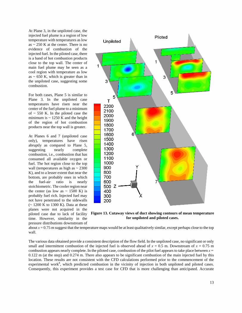
surface fits to the data is lower near the center of the measurement plane and higher near the edge. This uncertainty does not include the previously noted error in fuel rich regions of the flow, or any other non-statistical error. Figure 13 contains 3-dimensional cutaway views of the duct showing contour plots of the fitted temperature functions. Flow is from top left to bottom right. Recall that the main fuel injector is on the top wall between Planes 1 and 3, and the pilot injectors are in the top wall upstream of Plane 1. At Plane 1 in the unpiloted case the temperature is fairly uniform, between 1030 K and 1250 K. The mean temperature for all the data points of this plane and case is 1162 K. This mean compares favorably with the value computed assuming 1-D flow from the heater, which is 1187±60 K. In the piloted case, the temperature drops slightly close to the top wall where the (cold) pilot fuel is injected. There is no indication of combustion in this plane.

12

At Plane 3, in the unpiloted case, the injected fuel plume is a region of low temperature with temperatures as low as ~ 250 K at the center. There is no evidence of combustion of the injected fuel. In the piloted case, there is a band of hot combustion products close to the top wall. The center of main fuel plume may be seen as a cool region with temperature as low as ~ 650 K, which is greater than in the unpiloted case, suggesting some combustion.

For both cases, Plane 5 is similar to Plane 3. In the unpiloted case temperatures have risen near the center of the fuel plume to a minimum of ~ 550 K. In the piloted case the minimum is ~ 1250 K and the height of the region of hot combustion products near the top wall is greater. At Planes 6 and 7 (unpiloted case only), temperatures have risen abruptly as compared to Plane 5, suggesting nearly complete combustion, i.e., combustion that has consumed all available oxygen or fuel. The hot region close to the top wall (temperatures as high as ~ 2300 K), and to a lesser extent that near the bottom, are probably ones in which the fuel-air ratio is nearly stoichiometric. The cooler region near the center (as low as ~ 1500 K) is probably fuel rich. Injected fuel may not have penetrated to the sidewalls (~ 1200 K to 1300 K). Data at these planes were not acquired in the piloted case due to lack of facility time. However, similarity in the pressure distributions downstream of about x = 0.75 m suggest that the temperatwall.

F

The various data obtained provide a consismall and intermittent combustion of thecombustion appears nearly complete. In t0.122 m (at the step) and 0.274 m. Therelocation. These results are not consistenexperimental work8, which predicted coConsequently, this experiment provides

igure 13. Cutaway views of duct showing contours of mean temperaturefor unpiloted and piloted cases.

13

ure maps would be at least qualitatively similar, except perhaps close to the top

stent description of the flow field. In the unpiloted case, no significant or only injected fuel is observed ahead of x = 0.5 m. Downstream of x = 0.75 m

he piloted case, combustion of the pilot fuel appears to take place between x = also appears to be significant combustion of the main injected fuel by this t with the CFD calculations performed prior to the commencement of the mbustion in the vicinity of injection in both unpiloted and piloted cases. a test case for CFD that is more challenging than anticipated. Accurate

calculation will require accurate modeling of the chemical kinetics and turbulence-chemistry interactions as well as accurate modeling of the turbulent mixing. 8.5 SUMMARY Two experiments to acquire data for the validation of computational fluid dynamics (CFD) codes used in the design of supersonic combustors have been described. The first study was of a supersonic coaxial jet with center jet helium and coflowing jet air. Data include schlieren visualization, gas sampling and Pitot probe surveys, and RELIEF flow tagging velocity measurements. Calculations utilizing a structured finite difference code and Wilcox’s ω~

~−k model have been presented. Calculations demonstrated

non-physical discontinuities in slope of mole fraction and Pitot pressure due to inadequacies in the turbulence model. The second study was of a supersonic combustor with single downstream angled hydrogen fuel injector. Data include CARS temperature maps, and wall pressures and temperatures. Modern design of experiments techniques have been used to maximize data value. Contrary to the result of previously performed CFD calculations, it was found that (without pilot injectors) ignition did not occur until significantly downstream of injection. This is attributed to inadequacies in the kinetics model and/or the model for turbulence chemistry interaction. 8.6 ACKNOWLEDGEMENTS The 1st author would like to acknowledge the support of the NASA Langley Research Center through grant NCC1-370. 8.7 REFERENCES 1 Carty, A. A., Cutler, A. D., “Development and Validation of a Supersonic Helium-Air Coannular Jet Facility,” NASA CR-1999-209717, Nov 1999. 2 Cutler, A. D., Carty, A. A., Doerner, S. E., Diskin, G. S., Drummond, J. P., “Supersonic Coaxial Jet Experiment for CFD Code Validation,” AIAA Paper 99-3588, June 1999. 3 Cutler, A. D., White, J. A., “An Experimental and CFD Study of a Supersonic Coaxial Jet,” AIAA Paper 2001-0143, Jan 2001. 4 Diskin, G. S., “Experimental and Theoretical Investigation of the Physical Processes Important to the RELIEF Flow Tagging Diagnostic,” Ph.D. Dissertation, Princeton University, 1997. 5 Papamoschou, D., Roshko, A., “The compressible turbulent shear layer: an experimental study,” J. Fluid Mech., Vol 197, pp. 453-577, 1988. 6 White, J. A., Morrison, J. H., “A Pseudo-Temporal Multi-Grid Relaxation Scheme for Solving the Parabolized Navier-Stokes Equations,” AIAA Paper 99-3360, June 1999. 7 Cutler, A. D., Danehy, P. M., Springer, R. R., Deloach, R., Capriotti, D. P., “CARS Thermometry in a Supersonic Combustor for CFD Code Validation,” AIAA Paper 2002-0743, Jan. 2002. 8 Drummond, J. P., Diskin, G. S., Cutler, A. D., “Fuel-Air Mixing and Combustion in Scramjets,” Technologies for Propelled Hypersonic Flight, NATO Research and Technology Organization, Working Group 10, RTO Report AVT 10, January 2001. 9 Eckbreth, A. C., Laser Diagnostics for Combustion Temperature and Species, 2nd Ed., Combustion Science and Technology Series, Gordon and Breach, 1996. 10 Smith, M. W., Jarrett, O. Jr., Antcliff, R. R., Northam, G. B., Cutler, A. D., Taylor, D. J., “Coherent anti-Stokes Raman spectroscopy temperature measurements in a hydrogen-fueled supersonic combustor,” Journal of Propulsion and Power, Vol. 9, No. 2, 1993, pp. 163-168. 11 Cutler, A. D., Johnson, C. H., “Analysis of intermittency and probe data in a supersonic flow with injection,” Experiments in Fluids, Vol. 23, pp. 38-47, 1997.

14

15

12 Wilcox, D. C., Turbulence Modeling for CFD, 2nd Edition, DCW Industries, Inc., July 1998. 13 Direct-Connect Supersonic Combustion Facility, Facility Brochure, Wind Tunnel Enterprise, NASA Langley Research Center, www.wte.larc.nasa.gov. 14 Auslender, A. H., “An Application of Distortion Analysis to Scramjet Combustor Performance Assessment,” Final Report, 1996 JANNAF Propulsion and Joint Subcommittee Meeting Scramjet Performance Workshop, Dec. 12, 1996. 15 Springer, R. R., Cutler, A. D., Diskin, G. S., Smith, M. W., “Conventional/Laser Diagnostics to Assess Flow Quality in a Combustion-Heated Facility,” AIAA Paper 99-2170, 35th AIAA/ASME/SAE/ASEE Joint Propulsion Conference and Exhibit, Los Angeles, CA, June 20-24, 1999. 16 Eckbreth, A. C., “Optical Splitter for Dynamic Range Enhancement of Optical Multichannel Detectors,” Applied Optics, July 15, 1983. 17 Clark, G., Farrow, R. L., The CARSFT Code: User and Programmer Information, Sandia National Laboratories, Livermore, CA, Aug. 3, 1990. 18 Table Curve 3D Version 3.0 User’s Manual, AISN Software Inc., www.spss.com, 1997. 19 Box, G. E. P and Draper, N. R., Empirical Model Building and Response Surfaces, New York, John Wiley and Sons, 1987.