CHAPTER 6: FUEL-AIR MIXING AND COMBUSTION IN SCRAMJETS J. Philip Drummond and Glenn S. Diskin NASA Langley Research Center, Hampton, Virginia [email protected], [email protected]Andrew D. Cutler The George Washington University Joint Institute for Advancement of Flight Sciences, Hampton, Virginia [email protected]6.1 Introduction At flight speeds, the residence time for atmospheric air ingested into a scramjet inlet and exiting from the engine nozzle is on the order of a millisecond. Therefore, fuel injected into the air must efficiently mix within tens of microseconds and react to release its energy in the combustor. The overall combustion process should be mixing controlled to provide a stable operating environment; in reality, however, combustion in the upstream portion of the combustor, particularly at higher Mach numbers, is kinetically controlled where ignition delay times are on the same order as the fluid scale. Both mixing and combustion time scales must be considered in a detailed study of mixing and reaction in a scramjet to understand the flow processes and to ultimately achieve a successful design. Although the geometric configuration of a scramjet is relatively simple compared to a turbomachinery design, the flow physics associated with the simultaneous injection of fuel from multiple injector configura- tions, and the mixing and combustion of that fuel downstream of the injectors is still quite complex. For this reason, many researchers have considered the more tractable problem of a spatially developing, primarily supersonic, chemically reacting mixing layer or jet that relaxes only the complexities introduced by engine geometry. All of the difficulties introduced by the fluid mechanics, combustion chemistry, and interactions between these phenomena can be retained in the reacting mixing layer, making it an ideal problem for the detailed study of supersonic reacting flow in a scramjet. With a good understanding of the physics of the scramjet internal flowfield, the designer can then return to the actual scramjet geometry with this knowledge and apply engineering design tools that more properly account for the complex physics. This approach will guide the discussion in the remainder of this section. 6.2 Reacting Mixing Layers and Jets As described earlier, compressible shear/mixing layers and jets provide good model problems for studying the physical processes occurring in high-speed mixing and reacting flow in a scramjet. Mixing layers are characterized by large-scale eddies that form due to the high shear that is present between the fuel and air streams. These eddies entrain fuel and air into the mixing region. Stretching occurs in the interfacial region between the fluids leading to increased surface area and locally steep concentration gradients. Molecular diffusion then occurs across the strained interfaces. There has been a significant amount of experimental and numerical research to study mixing layer and jet flows [1]- [9]. For the same velocity and density ratios between fuel and air, increased compressibility, to the levels present in a scramjet, results in reduced mixing layer growth rates and reduced mixing. The level of compressibility in a mixing layer with air stream 1 and fuel stream 2 can be approximately characterized by the velocity ratio, r = U 2 /U 1 , the density ratio, 121 https://ntrs.nasa.gov/search.jsp?R=20060020221 2018-04-08T06:34:02+00:00Z
At flight speeds, the residence time for atmospheric air ingested into a scramjet inlet and exiting from theengine nozzle is on the order of a millisecond. Therefore, fuel injected into the air must efficiently mixwithin tens of microseconds and react to release its energy in the combustor. The overall combustion processshould be mixing controlled to provide a stable operating environment; in reality, however, combustion inthe upstream portion of the combustor, particularly at higher Mach numbers, is kinetically controlled whereignition delay times are on the same order as the fluid scale. Both mixing and combustion time scales mustbe considered in a detailed study of mixing and reaction in a scramjet to understand the flow processes andto ultimately achieve a successful design.
Although the geometric configuration of a scramjet is relatively simple compared to a turbomachinerydesign, the flow physics associated with the simultaneous injection of fuel from multiple injector configura-tions, and the mixing and combustion of that fuel downstream of the injectors is still quite complex. For thisreason, many researchers have considered the more tractable problem of a spatially developing, primarilysupersonic, chemically reacting mixing layer or jet that relaxes only the complexities introduced by enginegeometry. All of the difficulties introduced by the fluid mechanics, combustion chemistry, and interactionsbetween these phenomena can be retained in the reacting mixing layer, making it an ideal problem for thedetailed study of supersonic reacting flow in a scramjet. With a good understanding of the physics of thescramjet internal flowfield, the designer can then return to the actual scramjet geometry with this knowledgeand apply engineering design tools that more properly account for the complex physics. This approach willguide the discussion in the remainder of this section.
6.2 Reacting Mixing Layers and Jets
As described earlier, compressible shear/mixing layers and jets provide good model problems for studyingthe physical processes occurring in high-speed mixing and reacting flow in a scramjet. Mixing layers arecharacterized by large-scale eddies that form due to the high shear that is present between the fuel and airstreams. These eddies entrain fuel and air into the mixing region. Stretching occurs in the interfacial regionbetween the fluids leading to increased surface area and locally steep concentration gradients. Moleculardiffusion then occurs across the strained interfaces. There has been a significant amount of experimentaland numerical research to study mixing layer and jet flows [1]- [9]. For the same velocity and density ratiosbetween fuel and air, increased compressibility, to the levels present in a scramjet, results in reduced mixinglayer growth rates and reduced mixing. The level of compressibility in a mixing layer with air stream 1and fuel stream 2 can be approximately characterized by the velocity ratio, r = U2/U1, the density ratio,
s = ρ2/ρ1, and the convective Mach number,Mc = (U2−U1)/(a1+a2) where a is the speed of sound. Increasedcompressibility reorganizes the turbulence field and modifies the development of turbulent structures. Theresulting suppressed transverse Reynolds normal stresses appear to result in reduced momentum transport.In addition, the primary Reynolds shear stresses responsible for mixing layer growth rate also are reduced.The primary mixing layer instability becomes three-dimensional with a convective Mach number above 0.5,reducing the growth of the large scale eddies. Finally, the turbulent eddies become skewed, flat, and lessorganized as compressibility increases. All of these effects combine to reduce the growth rate of the mixinglayer and the overall level of mixing that is achieved.
Several phenomena result in the reduction of mixing with increasing flow velocity, including the velocitydifferential between fuel and air, and compressibility. Potentially, the existence of both high and low growthand mixing rates are possible, and the engine designer with an understanding of the flow physics controllingthese phenomena can advantageously use these effects. The shock and expansion wave structure in andabout the mixing layer can interact with the turbulence field to affect mixing layer growth [1]. Shock andexpansion waves interacting with the layer result from the engine internal structure. Experiments haveshown that the shocks that would result from wall and strut compressions appear to enhance the growthof the two-dimensional eddy structure (rollers) of a mixing layer. This effect is most pronounced when theduct height in the experiment and the shear layer width become comparable. Waves may be produced bythe mixing layer itself under appropriate conditions. Localized shocks (often termed shocklets) occur withinthe mixing layer when the accelerating flow over an eddy becomes supersonic even when the surroundingflow is subsonic. When the overall flow is supersonic, the eddy shocklets will extend as shocks into the flowbeyond the individual eddies. These shocklets can retard eddy growth due to increased localized pressurearound the eddy.
The growth of a mixing layer produces a displacement effect on the surrounding flow field. This displace-ment in confined flow produces pressure gradients that can affect the later development of the mixing layer,typically retarding growth. When chemical reaction occurs in a mixing layer, resulting in heat release, thegrowth of the mixing layer is retarded in both subsonic and supersonic flow [1, 2]. The effect of heat releasecan also vary spatially as a function of the local stoichiometry and chemical reaction. The retarded growthin both instances can be reversed, however, by allowing the bounding wall to diverge relative to the initialwall angles where retarded growth was noted [1]. While the process of mixing layer growth is affected by thecombustor geometry and design, fuel injector design carried out with proper consideration for the inlet andcombustor geometry can have a strong influence on overall mixing and combustion efficiency. Considerableeffort has been expended over the past fifteen years to achieve efficient fuel injector designs. Injector designwill be considered in the next section.
6.3 Scramjet Fuel Injectors
There are several key issues that must be considered in the design of an efficient fuel injector. Of particularimportance are the total pressure losses created by the injector and the injection processes, that must beminimized since the losses reduce the thrust of the engine. The injector design also must produce rapidmixing and combustion of the fuel and air. Rapid mixing and combustion allow the combustor length andweight to be minimized, and they provide the heat release for conversion to thrust by the engine nozzle.The fuel injector distribution in the engine also should result in as uniform a combustor profile as possibleentering the nozzle so as to produce an efficient nozzle expansion process. At moderate flight Mach numbers,up to Mach 10, fuel injection may have a normal component into the flow from the inlet, but at higher Machnumbers, the injection must be nearly axial since the fuel momentum provides a significant portion of theengine thrust. Intrusive injection devices can provide good fuel dispersal into the surrounding air, but theyrequire active cooling of the injector structure. The injector design and the flow disturbances produced byinjection also should provide a region for flameholding, resulting in a stable piloting source for downstreamignition of the fuel. The injector cannot result in too severe a local flow disturbance, that could result inlocally high wall static pressures and temperatures, leading to increased frictional losses and severe wallcooling requirements.
A number of options are available for injecting fuel and enhancing the mixing of the fuel and air in
122
high-speed flows typical of those found in a scramjet combustor [10, 11]. Two traditional approaches forinjecting fuel include injection from the combustor walls and in-stream injection from struts. The simplestapproach for wall injection involves the transverse injection of the fuel from wall orifices. Transverse injectorsoffer relatively rapid near-field mixing and good fuel penetration. Penetration of the fuel stream into thecross-flow is governed by the jet-to-freestream momentum flux ratio. The fuel jet interacts strongly with thecross-flow, producing a bow shock and a localized highly three-dimensional flow field. Resulting upstreamand downstream wall flow separations also provide regions for radical production and flameholding, but theycan also result in locally high wall heat transfer. Compressibility effects that were noted earlier for mixinglayer flows also are evident in the mixing regime downstream of a transverse jet. Compressibility againretards eddy growth and breakup in the mixing layer and suppresses entrainment of fuel and air, resultingin a reduction in mixing and reaction.
Improved mixing has also been achieved using alternative wall injector designs. Wall injection using geo-metrical shapes that introduce axial vorticity into the flow field has been successful. Vorticity can be inducedinto the fuel stream using convoluted surfaces or small tabs at the exit of the fuel injector. Alternatively,vorticity can be introduced into the air upstream of the injector using wedge shaped bodies placed on thecombustor walls. Vorticity addition to the air stream provides more significant mixing enhancement of fueland air [12]. When strong pressure gradients are present in the flowfield, e.g. at a shock, vorticity alignedwith the flow can be induced at a fuel-air interface, where a strong density gradient exists, by virtue of thebaroclinic torque. Fuel injection ramps have proven to be an effective means for fuel injection in a scramjetengine [2]. Fuel is injected from the base of the ramp. The unswept ramp configuration provides nearlystreamwise injection of fuel to produce a thrust component. The effects of angled injection on axial thrustonly go as the cosine of the angle, so small injection angles result in little loss in thrust. Flow separation atthe base of the ramp provides a region for flame holding and flame stabilization through the buildup of aradical pool. The ramp itself produces streamwise vorticity as the air stream sheds off of its edges, improvingthe downstream mixing. The swept ramp design provides all of the features of the unswept ramp, but thesweep results in better axial vorticity generation and mixing. A novel variation on the swept wedge injector,termed the aero-ramp injector [13], utilizes three arrays of injector nozzles at various inclination and yawangles to approximate the physical swept ramp design.
In-stream injection also has been utilized for fuel injection in a scramjet. Traditional approaches involvefuel injection from the sides and the base of an in-stream strut. Transverse injection results in behavior similarto transverse fueling from the wall, although differences can occur due to much thinner boundary layers onthe strut. Injection from the base of the strut results in slower mixing as compared to transverse injection. Acombination of transverse and streamwise injection, varied over the flight Mach number range, often has beenutilized to control reaction and heat release in a scramjet combustor. As noted earlier, however, streamwiseinjection has the advantage of adding to the thrust component of the engine. To increase the mixing fromstreamwise injectors, many of the approaches used to improve wall injection, including non-circular orifices,tabs, and ramps, have been successfully utilized. Several new concepts have emerged as well. Pulsed injectionusing either mechanical devices or fluidic oscillation techniques have shown promise for improved mixing.Pulsed injection of fuel utilizing a shuttering technique to control injection has been shown to improvemixing [12]. Fuel injection schemes integrated with cavities also provide the potential for improved mixingand flameholding. This type of integrated fuel injection/flameholding device, utilizing fuel injection intoa cavity and from its base, integrates the fuel injection with a cavity that provides flameholding, flamestabilization, and mixing enhancement if the cavity is properly tuned. Air exchange rates with the cavitymay be low, however, limiting the amount of fuel that can be added. Additional scramjet fuel injector designscontinue to be introduced and studied to achieve even higher levels of mixing and combustion efficiency.
Scramjet design is built upon both experimental and computational research. To assure that computa-tional tools properly represent the complex flow physics in a scramjet, careful evaluation of the computationaltools is necessary. Benchmark experiments are becoming available that provide the necessary data for evalu-ating the accuracy of the numerical algorithms and the physical models that the computational tools employ.In addition, these experiments provide in some instances the information necessary to improve the modelingemployed by the codes. Two experiments available for assessing high-speed combustion codes are describedin the next section. Results obtained from the application of a combustion code to these experiments arealso shown and discussed.
123
18.261.59
60.47
10.5010.00 15.87
Static pressure tap
76.20
25.40
19.84
15.88
41.91
152.27 Pref, CJ
Helium / 5% Oxygenor Air Tt, CJ
48.01
246.39
Center jet pressure tap
Plenumpressure tapPref, coflow
All dimensions in mm
Screens
AirTt, coflow
24.61
12.66
Figure 1: Coaxial jet assembly cross-section
6.4 Mixing and Combustion Experiments
Two basic experiments are being conducted at the NASA Langley Research Center to collect detailed high-speed mixing and combustion data for use in physical model development and code validation. The firstexperiment concerns coaxial jet mixing of a helium/oxygen center jet with a coflowing air outer jet andwas chosen to provide detailed supersonic mixing data. The second experiment was developed to studyhigh-speed mixing and combustion in a simple “scramjet like” engine environment. The experiment utilizesa ducted flow rig containing vitiated supersonic air with a single fuel injector that introduces supersonicgaseous hydrogen from the lower wall. Detailed wall and in flow surveys and noninterference diagnostics areused in both experiments. These experiments will be described in the following sections.
6.4.1 Coaxial Jet Mixing Experiment
A coaxial jet mixing experiment has been developed to study the high-speed compressible mixing of heliumand air. Details of the experiment are described in references [14] and [15]. The low-density helium, whichserves as a simulant of hydrogen fuel, was chosen to allow detailed studies of mixing without chemicalreaction. Oxygen is added to the helium jet as a diagnostic aid for an oxygen flow-tagging technique(RELIEF). Several methods are utilized to characterize the flow field including Schlieren visualization, pitotpressure, total temperature, and gas sampling probe surveying, and RELIEF velocimetry. A schematic ofthe coaxial jet configuration is shown in Figure 1. The rig consists of a 10 mm inner nozzle from whichhelium, mixed with 5 percent oxygen by volume, is injected at Mach 1.8 and an outer nozzle 60 mm indiameter from which coflowing air is introduced also at Mach 1.8. The velocity ratio between the two jets is2.25, the convective Mach number is 0.7, and the jet exit pressures are matched to one atmosphere.
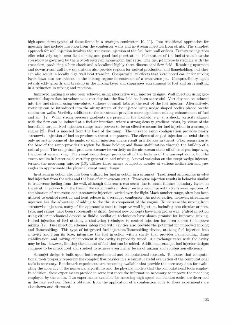
The resulting flow downstream of the nozzles can be seen in Figure 2, which shows a Schlieren image ofthe flowfield. The development of the mixing layer between the central helium jet and the air jet can be
124
Figure 2: Schlieren image of coaxial jet mixing (conical extension cap removed)
seen along with the shear layer development between the air jet and the surrounding quiescent laboratoryair into which the air jet exhausts. Shock-expansion wave structure emanating outward from the centerbodynozzle lip can also be seen. Inward propagating waves from the inner lip, due to the finite thickness of the lip(0.25 mm), can be observed in the air jet once they pass through the helium jet. These waves are not visiblein the helium jet due to the low refractive index within the center jet. A third wave can also be observedemanating inward from the outer nozzle lip and traversing both the air jet and the helium jet. Additionalresults from the experiment will also be considered later in this section when comparisons of the measureddata with numerical simulations are made.
6.4.2 SCHOLAR Combustor Experiment
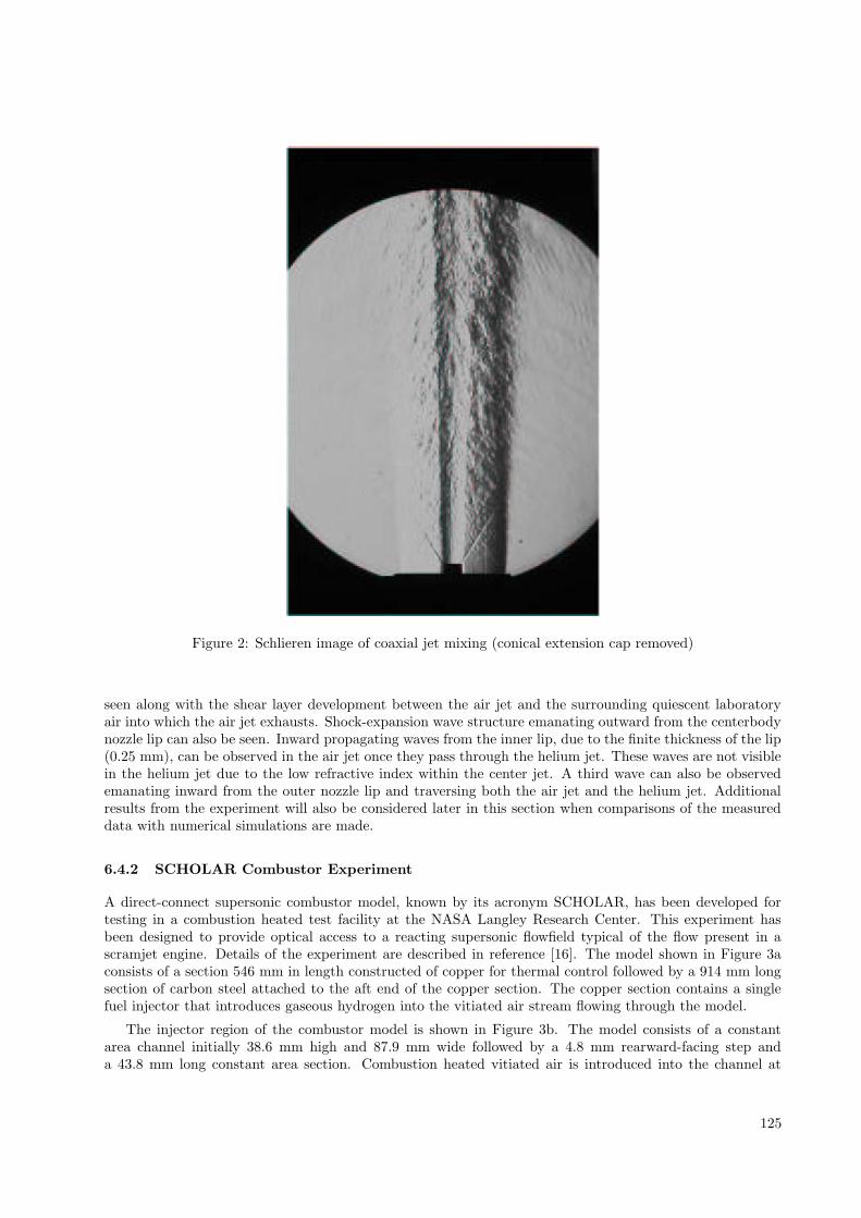
A direct-connect supersonic combustor model, known by its acronym SCHOLAR, has been developed fortesting in a combustion heated test facility at the NASA Langley Research Center. This experiment hasbeen designed to provide optical access to a reacting supersonic flowfield typical of the flow present in ascramjet engine. Details of the experiment are described in reference [16]. The model shown in Figure 3aconsists of a section 546 mm in length constructed of copper for thermal control followed by a 914 mm longsection of carbon steel attached to the aft end of the copper section. The copper section contains a singlefuel injector that introduces gaseous hydrogen into the vitiated air stream flowing through the model.
The injector region of the combustor model is shown in Figure 3b. The model consists of a constantarea channel initially 38.6 mm high and 87.9 mm wide followed by a 4.8 mm rearward-facing step anda 43.8 mm long constant area section. Combustion heated vitiated air is introduced into the channel at
125
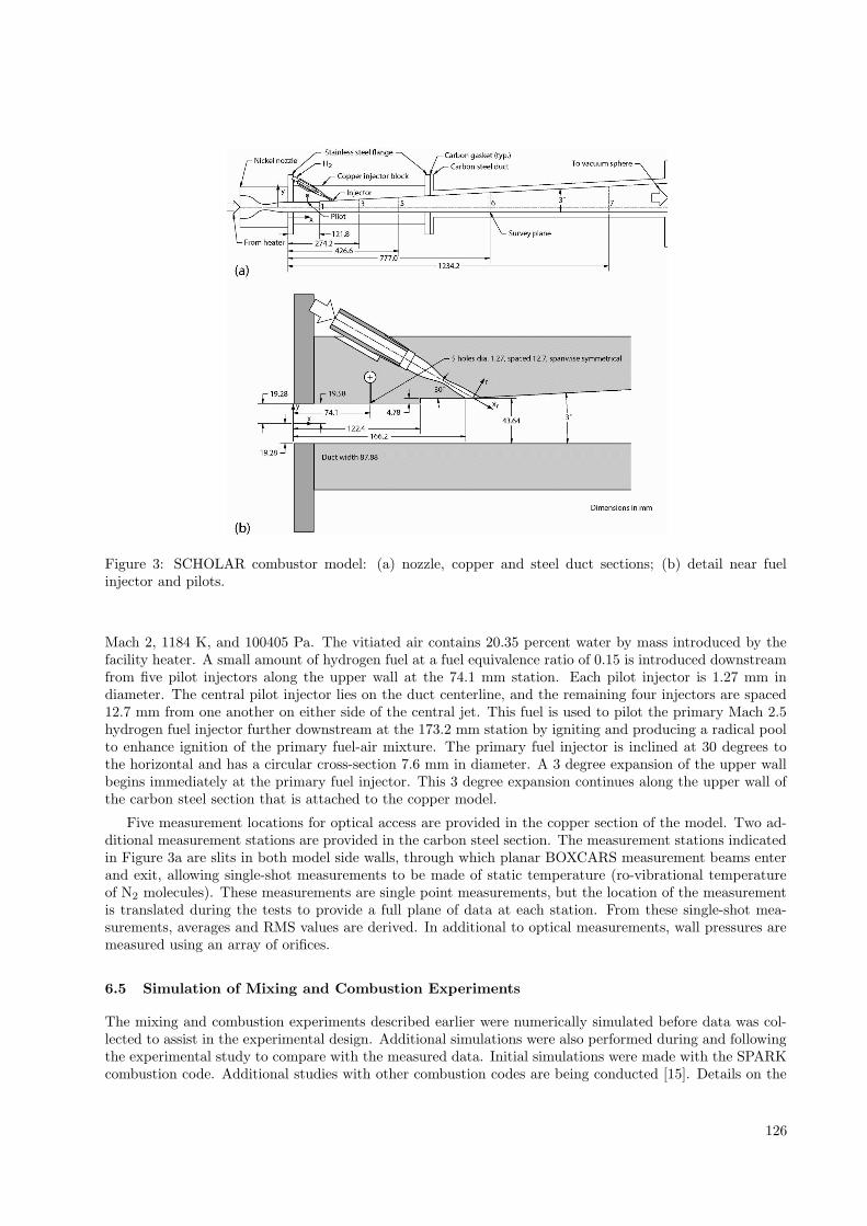
Figure 3: SCHOLAR combustor model: (a) nozzle, copper and steel duct sections; (b) detail near fuelinjector and pilots.
Mach 2, 1184 K, and 100405 Pa. The vitiated air contains 20.35 percent water by mass introduced by thefacility heater. A small amount of hydrogen fuel at a fuel equivalence ratio of 0.15 is introduced downstreamfrom five pilot injectors along the upper wall at the 74.1 mm station. Each pilot injector is 1.27 mm indiameter. The central pilot injector lies on the duct centerline, and the remaining four injectors are spaced12.7 mm from one another on either side of the central jet. This fuel is used to pilot the primary Mach 2.5hydrogen fuel injector further downstream at the 173.2 mm station by igniting and producing a radical poolto enhance ignition of the primary fuel-air mixture. The primary fuel injector is inclined at 30 degrees tothe horizontal and has a circular cross-section 7.6 mm in diameter. A 3 degree expansion of the upper wallbegins immediately at the primary fuel injector. This 3 degree expansion continues along the upper wall ofthe carbon steel section that is attached to the copper model.
Five measurement locations for optical access are provided in the copper section of the model. Two ad-ditional measurement stations are provided in the carbon steel section. The measurement stations indicatedin Figure 3a are slits in both model side walls, through which planar BOXCARS measurement beams enterand exit, allowing single-shot measurements to be made of static temperature (ro-vibrational temperatureof N2 molecules). These measurements are single point measurements, but the location of the measurementis translated during the tests to provide a full plane of data at each station. From these single-shot mea-surements, averages and RMS values are derived. In additional to optical measurements, wall pressures aremeasured using an array of orifices.
6.5 Simulation of Mixing and Combustion Experiments
The mixing and combustion experiments described earlier were numerically simulated before data was col-lected to assist in the experimental design. Additional simulations were also performed during and followingthe experimental study to compare with the measured data. Initial simulations were made with the SPARKcombustion code. Additional studies with other combustion codes are being conducted [15]. Details on the
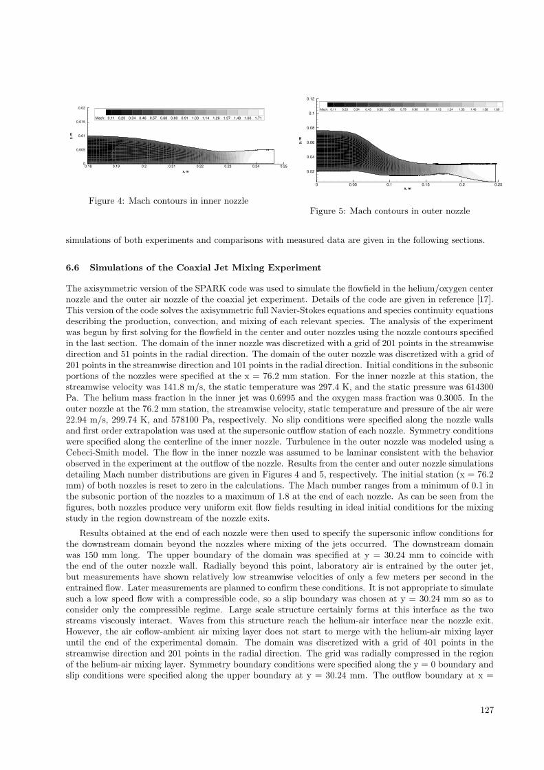
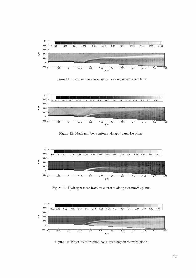
simulations of both experiments and comparisons with measured data are given in the following sections.
6.6 Simulations of the Coaxial Jet Mixing Experiment
The axisymmetric version of the SPARK code was used to simulate the flowfield in the helium/oxygen centernozzle and the outer air nozzle of the coaxial jet experiment. Details of the code are given in reference [17].This version of the code solves the axisymmetric full Navier-Stokes equations and species continuity equationsdescribing the production, convection, and mixing of each relevant species. The analysis of the experimentwas begun by first solving for the flowfield in the center and outer nozzles using the nozzle contours specifiedin the last section. The domain of the inner nozzle was discretized with a grid of 201 points in the streamwisedirection and 51 points in the radial direction. The domain of the outer nozzle was discretized with a grid of201 points in the streamwise direction and 101 points in the radial direction. Initial conditions in the subsonicportions of the nozzles were specified at the x = 76.2 mm station. For the inner nozzle at this station, thestreamwise velocity was 141.8 m/s, the static temperature was 297.4 K, and the static pressure was 614300Pa. The helium mass fraction in the inner jet was 0.6995 and the oxygen mass fraction was 0.3005. In theouter nozzle at the 76.2 mm station, the streamwise velocity, static temperature and pressure of the air were22.94 m/s, 299.74 K, and 578100 Pa, respectively. No slip conditions were specified along the nozzle wallsand first order extrapolation was used at the supersonic outflow station of each nozzle. Symmetry conditionswere specified along the centerline of the inner nozzle. Turbulence in the outer nozzle was modeled using aCebeci-Smith model. The flow in the inner nozzle was assumed to be laminar consistent with the behaviorobserved in the experiment at the outflow of the nozzle. Results from the center and outer nozzle simulationsdetailing Mach number distributions are given in Figures 4 and 5, respectively. The initial station (x = 76.2mm) of both nozzles is reset to zero in the calculations. The Mach number ranges from a minimum of 0.1 inthe subsonic portion of the nozzles to a maximum of 1.8 at the end of each nozzle. As can be seen from thefigures, both nozzles produce very uniform exit flow fields resulting in ideal initial conditions for the mixingstudy in the region downstream of the nozzle exits.
Results obtained at the end of each nozzle were then used to specify the supersonic inflow conditions forthe downstream domain beyond the nozzles where mixing of the jets occurred. The downstream domainwas 150 mm long. The upper boundary of the domain was specified at y = 30.24 mm to coincide withthe end of the outer nozzle wall. Radially beyond this point, laboratory air is entrained by the outer jet,but measurements have shown relatively low streamwise velocities of only a few meters per second in theentrained flow. Later measurements are planned to confirm these conditions. It is not appropriate to simulatesuch a low speed flow with a compressible code, so a slip boundary was chosen at y = 30.24 mm so as toconsider only the compressible regime. Large scale structure certainly forms at this interface as the twostreams viscously interact. Waves from this structure reach the helium-air interface near the nozzle exit.However, the air coflow-ambient air mixing layer does not start to merge with the helium-air mixing layeruntil the end of the experimental domain. The domain was discretized with a grid of 401 points in thestreamwise direction and 201 points in the radial direction. The grid was radially compressed in the regionof the helium-air mixing layer. Symmetry boundary conditions were specified along the y = 0 boundary andslip conditions were specified along the upper boundary at y = 30.24 mm. The outflow boundary at x =
Figure 6: Helium mass fraction contours downstream of nozzles
150 mm remained supersonic, and extrapolation conditions were specified at this location. Turbulence wasmodeled in the downstream domain with the turbulent jet mixing model of Eggers and Eklund [18, 19].
Results from the downstream calculation are shown in Figures 6 through 8. Helium-air mixing down-stream of the nozzles is shown in Figure 6. The helium mass fraction in the figure ranges from a minimumof zero to a maximum of approximately 0.7. There is significant mixing of the helium and air throughoutthe downstream region although relatively high mass fractions of helium still remain near the centerline.
A comparison of the measured helium mass fraction data with the simulation results at several stationsdownstream of the nozzles is given in Figure 7. Agreement between the simulation and the data is very goodat each station. The code somewhat overpredicts the mixing near the centerline at the x = 0.12 m station,although the prediction improves with increasing radial distance. A comparison of measured pitot pressureswith the simulation is shown in Figure 8. Agreement is good in the region of the air coflowing jet, but thesimulation somewhat overpredicts the pitot pressure in the helium-air mixing region. The comparison withthe experimental data differs at large radial distances greater than 0.025 m as the code does not considerthe effects of the laboratory air entrained by the coaxial air jet. The RELIEF streamwise velocity data iscompared with the simulation in Figure 9. The prediction agrees well with the data at the first three stationsand slightly overpredicts the data at the remaining stations near the centerline. The simulation somewhatunderpredicts the the velocity at the final three stations in the mixing region between the helium and aircoflowing jets in agreement with the pitot pressure results.
6.6.1 Simulations of the SCHOLAR Combustor Experiment
The three-dimensional version of the SPARK code was used to simulate the flowfield in the SCHOLARcombustor model. Details of the code are given in the references [17, 20]. This version of the code solvesthe 3-D full Navier-Stokes equations and species continuity equations describing the production, convection,and mixing of chemical species. Calculations have been used in the design and refinement of the experiment.In the calculation the model was rotated from the orientation shown in Figure 3 such that the injector wallwas aligned with the lower computational boundary.
Calculations were begun at the x = 0 station of the SCHOLAR model where vitiated air from the facilityenters the duct. Vitiated air entered the model at Mach 2.0 yielding a velocity of 1395.7 m/s, a statictemperature of 1184 K, and a static pressure of 100405 Pa. The calculated equilibrium mole fractions of thespecies present in the vitiated air, determined by a quasi-one-dimensional nozzle code, are given in Table 1.
The initial channel cross-section is 38.6 mm high and 87.9 mm wide. The hydrogen fuel injector introduces
Figure 10: Static pressure contours along streamwise plane
hydrogen through a choked nozzle at Mach 2.5, a static temperature of 134.2 K, and a static pressure of201300 Pa. The pilot fuel injectors described earlier were activated to improve flameholding under thepresent test conditions. The pilot injectors are assumed to be choked at the wall surface, resulting in a statictemperature and pressure of 251.7 K and 722535 Pa, respectively. No slip conditions were specified alongthe upper, lower, and near- and far-side channel walls. First order extrapolation was used at the supersonicoutflow station located at the 546 mm station for this calculation. This domain was discretized with a grid of401 points in the streamwise direction, 61 points in the cross-stream direction, and 121 points in the spanwisedirection. The grid was compressed near the solid walls and the fuel injector. Turbulence was modeled in thenear wall region using the Bauldwin-Lomax model, and in the interior field using the turbulent jet mixingmodel [18, 19]. Chemistry was modeled using the 9 species, 18 reaction model described in reference [17].This model provides a detailed description of hydrogen-air chemistry, but does not consider the effects ofthe small quantities of oxides of nitrogen and hydrocarbon species present in the vitiated air.
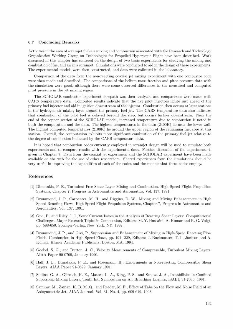
The results of flowfield simulations of the SCHOLAR combustor model are shown in Figures 10-16.Figure 10 shows static pressure contours along the streamwise plane centered on the fuel jet. Traversingthe combustor from inflow to outflow, a weak bow shock produced by the pilot injectors can be seen. Thispressure rise is communicated through the wall boundary layer resulting in a weak shock at the inflow tothe combustor. This is followed by the expansion of the flow over the lower wall step. Just downstream,the flow is compressed through a recompression shock followed by a strong bow shock lying ahead of theprimary fuel injector. Both the fuel jet and its surrounding air flow then expand beyond the fuel injector.The reflection of the bow shock interacts with the low density hydrogen fuel jet altering the shock angle.Figure 11 shows the static temperature contours along the same streamwise plane. The temperature riseassociated with combustion of the pilot fuel near the primary fuel injector, and combustion of the shear layerof the primary injector plume can also be seen. Figure 12 shows the resulting Mach number contours along
Figure 14: Water mass fraction contours along streamwise plane
131
y, m
z,m
0 0.01 0.02 0.03 0.04 0.05 0.06 0.07 0.08 0.09
-0.01
0
0.01
0.02
0.03
0.04
0.05H2: 0.01 0.04 0.07 0.10 0.13 0.16 0.19 0.21
Figure 15: Hydrogen mass fraction at downstreamstation (0.427 m)
y, m
z,m
0 0.01 0.02 0.03 0.04 0.05 0.06 0.07 0.08 0.09
-0.01
0
0.01
0.02
0.03
0.04
0.05H2O: 0.22 0.25 0.28 0.31 0.34 0.36 0.39 0.42
Figure 16: Water mass fraction at downstream sta-tion (0.427 m)
the streamwise plane. In addition to the above features, the wall boundary layers can be seen along withregions of recirculation located behind the lower wall step and where the bow shock interacts with the upperwall boundary layer. The plume of the fuel jet can also be seen. Figure 13 also displays the jet in terms ofmass fraction contours of hydrogen along the streamwise plane. Figure 14 shows contours of the water massfraction produced as a result of chemical reaction of the hydrogen fuel and air. The contours range from aminimum mass fraction of zero in the hydrogen jet core to a maximum mass fraction of 0.46 including thewater introduced in the air from facility vitiation.
Figures 15 and 16 show contours of hydrogen and water mass fraction, respectively, in a cross-plane atthe 0.427 m station bounded by the channel walls. Values of the hydrogen mass fraction range from zero to0.23 with the highest concentrations existing only in the immediate jet core. Significant amounts of hydrogenhave been mixed with facility air and consumed downstream by reaction. Values of the water contours againrange from a minimum mass fraction of 0.203 (from vitiation) to a maximum mass fraction of 0.44. Vorticesthat form as the facility air interacts with the fuel jet lift and spread the jet enhancing fuel-air mixing andreaction. The vortices also convect fluid toward the lower wall and into the remaining fuel jet.
Comparisons of the measured and computed static temperatures at three stations in the copper sectionof the SCHOLAR model are given in Figures 17 through 19. These stations correspond to stations 1, 3, and5 in Figure 3a. Measurements were not made for the piloted runs at stations 6 and 7 in the steel section ofthe SCHOLAR model. Figure 17 shows results at the step in the model wall. The computed results show arise in temperature ranging from 400K on the walls to 1299K where the pilot fuel is mixing with the facilityair and heating, but not undergoing combustion. The measured data ranges from 850K to 1200K in the flowwith the fuel and air mixing but not reacting. The asymmetry of the data may simply be attributed to thecoarseness of the grid used in surveying the flow relative to the scale of the flow features combined with theslightly asymmetrical location of the grid with respect to the flow. There is no suggestion that the flow itselfis not symmetrical. At the 0.274 m station shown in Figure 18, the data now indicate combustion of thepilot fuel whereas the computation shows combustion of the pilot fuel and initial combustion of the primaryinjector fuel. The computation and the data indicate a maximum temperature of around 2030K and 2300K,respectively. A “cold” core of hydrogen still persists in both the data and the calculation. Figure 19 showsresults at the 0.427 m station. Further combustion of the primary injector fuel in the mixing layer betweenthe hydrogen and the facility air is indicated in the calculation. The data indicates increased combustionand temperature rise of the pilot fuel and on the lower surface of the primary injector hydrogen-air mixinglayer. No combustion of the fuel is seen in the data along the upper surface of the primary fuel jet at thislocation.
Figure 19: Comparison of computed static temperature (left) with data at 0.427 m station
133
6.7 Concluding Remarks
Activities in the area of scramjet fuel-air mixing and combustion associated with the Research and TechnologyOrganization Working Group on Technologies for Propelled Hypersonic Flight have been described. Workdiscussed in this chapter has centered on the design of two basic experiments for studying the mixing andcombustion of fuel and air in a scramjet. Simulations were conducted to aid in the design of these experiments.The experimental models were then constructed, and data were collected in the laboratory.
Comparison of the data from the non-reacting coaxial jet mixing experiment with one combustor codewere then made and described. The comparisons of the helium mass fraction and pitot pressure data withthe simulation were good, although there were some observed differences in the measured and computedpitot pressure in the jet mixing region.
The SCHOLAR combustor experiment flowpath was then analyzed and comparisons were made withCARS temperature data. Computed results indicate that the five pilot injectors ignite just ahead of theprimary fuel injector and aid in ignition downstream of the injector. Combustion then occurs at later stationsin the hydrogen-air mixing layer around the primary fuel jet. The CARS temperature data also indicatesthat combustion of the pilot fuel is delayed beyond the step, but occurs further downstream. Near theend of the copper section of the SCHOLAR model, increased temperature due to combustion is noted inboth the computation and the data. The highest temperatures in the data (2400K) lie near the lower wall.The highest computed temperatures (2100K) lie around the upper region of the remaining fuel core at thisstation. Overall, the computation exhibits more significant combustion of the primary fuel jet relative tothe degree of combustion indicated by the CARS temperature data.
It is hoped that combustion codes currently employed in scramjet design will be used to simulate bothexperiments and to compare results with the experimental data. Further discussion of the experiments isgiven in Chapter 7. Data from the coaxial jet experiment and the SCHOLAR experiment have been madeavailable on the web for the use of other researchers. Shared experiences from the simulations should bevery useful in improving the capabilities of each of the codes and the models that these codes employ.
References
[1] Dimotakis, P. E., Turbulent Free Shear Layer Mixing and Combustion. High Speed Flight PropulsionSystems, Chapter 7, Progress in Astronautics and Aeronautics, Vol. 137, 1991.
[2] Drummond, J. P., Carpenter, M. H., and Riggins, D. W., Mixing and Mixing Enhancement in HighSpeed Reacting Flows. High Speed Flight Propulsion Systems, Chapter 7, Progress in Astronautics andAeronautics, Vol. 137, 1991.
[3] Givi, P., and Riley, J. J., Some Current Issues in the Analysis of Reacting Shear Layers: ComputationalChallenges. Major Research Topics in Combustion, Editors: M. Y. Hussaini, A. Kumar and R. G. Voigt,pp. 588-650, Springer-Verlag, New York, NY, 1992.
[4] Drummond, J. P., and Givi, P., Suppression and Enhancement of Mixing in High-Speed Reacting FlowFields. Combustion in High-Speed Flows, pp. 191- 229, Editors: J. Buckmaster, T. L. Jackson and A.Kumar, Kluwer Academic Publishers, Boston, MA, 1994.
[5] Goebel, S. G., and Dutton, J. C., Velocity Measurements of Compressible, Turbulent Mixing Layers.AIAA Paper 90-0709, January 1990.
[6] Hall, J. L., Dimotakis, P. E., and Rosemann, H., Experiments in Non-reacting Compressible ShearLayers. AIAA Paper 91-0629, January 1991.
[7] Sullins, G. A., Gilreath, H. E., Mattes, L. A., King, P. S., and Schetz, J. A., Instabilities in ConfinedSupersonic Mixing Layers. Tenth Int. Symposium on Air Breathing Engines, ISABE 91-7096, 1991.
[8] Samimy, M., Zaman, K. B. M .Q., and Reeder, M. F., Effect of Tabs on the Flow and Noise Field of anAxisymmetric Jet. AIAA Journal, Vol. 31, No. 4, pp. 609-619, 1993.
134
[9] Cox, S. K., Fuller, R. P., Schetz, J. A., and Walters, R. W., Vortical Interactions Generated by anInjector Array to Enhance Mixing in Supersonic Flow. AIAA Paper 94-0708, January 1994.
[10] Seiner, J. M., Dash, S. M., and Kenzakowski, D. C., Historical Survey on Enhanced Mixing in ScramjetEngines. AIAA Paper 99-4869, August 1999.
[11] Bogdanoff, D. W., Advanced Injection and Mixing Techniques for Scramjet Combustors. AIAA Journalof Propulsion and Power, Vol. 10, No. 2, pp. 183-190, 1994.
[12] Cutler, A. D., Harding, G. C., and Diskin, G. S., High Frequency Supersonic Pulsed Injection. AIAAPaper 2001-0517, January 2001.
[13] Schetz, J. A., Cox-Stouffer, S. K., and Fuller, R. P., Integrated CFD and Experimental Studies ofComplex Injectors in Supersonic Flows. AIAA Paper 98-2780, June 1998.
[14] Cutler, A. D., Carty, A., Doerner, S., Diskin, G., and Drummond, J. P., Supersonic Coaxial Jet FlowExperiment for CFD Code Validation. AIAA Paper 99-3588, June 1999.
[15] Cutler, A. D., and White, J. A., An Experimental and CFD Study of a Supersonic Coaxial Jet. AIAAPaper 2001-0143, January 2001.
[16] Cutler, A., Danehy, P. M., Springer, R. R., and DeLoach, D. P., CARS Thermometry in a SupersonicCombustor for CFD Code Validation. AIAA Paper 2002-0743, January 2002.
[17] Drummond, J. P., Numerical Simulation of a Supersonic Chemically Reacting Mixing Layer. NASA TM4055, 1988.
[18] Eggers, J. M., Turbulent Mixing of Coaxial Compressible Hydrogen-Air Jets. NASA TN D-6487, 1971.
[19] Eklund, D. R., et al., Computational/ Experimental Investigation of Staged Injection into a Mach 2Flow. AIAA Journal, Vol. 32, No. 5, pp. 907-916, 1994.
[20] Carpenter, M. H., Three-Dimensional Computations of Cross-Flow Injection and Combustion in a Su-personic Flow. AIAA Paper 89-1870, June 1989.