Modeling-Science June 3, 2008 Chapter Five Continuous Time Models The purpose of computing is insight, not numbers. Richard Hamming We study models for continuous systems which can be expressed using ordinary differential equations. We cover interesting models in dimensions one and two, but also higher-dimensional problems that involve differentiat- ing arrays. We introduce powerful graphic and numeric tools embedded in EJS, and study new visualizations such as direction fields and phase-space plots. 5.1 THE COOLING COFFEE PROBLEM Figure 5.1: Comparison of Newton’s law of proportional cooling with exper- imental data of the cooling of a cup of black coffee (top plot) and of coffee with cream. The model data (continuous line) fits well with the experimen- tal data (square marks). Project 5.1 shows how to read an experimental data file. You are about to give a short presentation of your latest computer simulation to your professor when two freshly brewed cups of coffee arrive. You both decide to wait until the end of the presentation (5 minutes) to drink your coffees but your professor immediately adds some cream to her
Transcript
Modeling-Science June 3, 2008
Chapter Five
Continuous Time Models
The purpose of computing is insight, not numbers. RichardHamming
We study models for continuous systems which can be expressed usingordinary differential equations. We cover interesting models in dimensionsone and two, but also higher-dimensional problems that involve differentiat-ing arrays. We introduce powerful graphic and numeric tools embedded inEJS, and study new visualizations such as direction fields and phase-spaceplots.
5.1 THE COOLING COFFEE PROBLEM
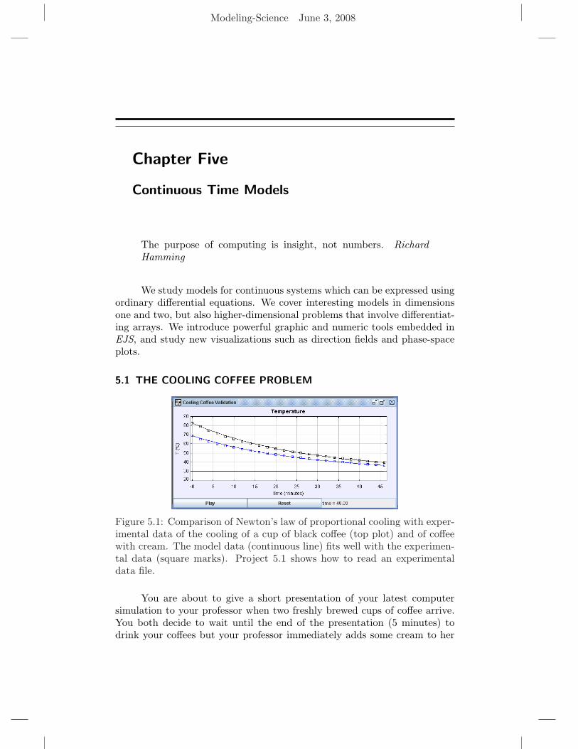
Figure 5.1: Comparison of Newton’s law of proportional cooling with exper-imental data of the cooling of a cup of black coffee (top plot) and of coffeewith cream. The model data (continuous line) fits well with the experimen-tal data (square marks). Project 5.1 shows how to read an experimentaldata file.
You are about to give a short presentation of your latest computersimulation to your professor when two freshly brewed cups of coffee arrive.You both decide to wait until the end of the presentation (5 minutes) todrink your coffees but your professor immediately adds some cream to her
Modeling-Science June 3, 2008
62 CHAPTER 5
coffee while you wait until the end of your presentation. Your presentationwent well but you wonder who will drink a hotter coffee. Curiosity is a basicingredient of science and asking what, why, and how things happen leads toa deeper understanding of how nature works. Your question makes a perfectcase for modeling, the central theme of this book.
In 1958 two Cornell University engineering students presented a re-port title “The Mechanisms of Cooling Hot Quiescent Liquids” in whichthey studied the effect of adding cream to a cup of hot coffee. Because typi-cal brewing temperature for coffee is 85C (185F) and drinking temperatureis 62C (143F), they studied the effect of adding cream when the coffee isserved or adding it just before it is consumed. This is not a trivial prob-lem because a hot body exchanges heat with its surroundings through thesimultaneous processes of conduction, convection, evaporation, and radia-tion. Newton argued that since the thermal energy is proportional to thevolume and the energy loss is proportional to the exposed area, the timeof cooling is proportional to the diameter. Larger objects therefore coolmore slowly. Laplace, Helmholtz, and Kelvin extended Newton’s model byconsidering gravitational energy and radiation to estimate the age of theSun to be well over 20 million years. Although the discovery of nuclearfusion greatly increased this age estimate, the balance between cooling andthermonuclear fusion is of fundamental importance in stellar models. Todaywe use advanced heating, cooling, and energy transport models to debatethe impact of global warming. Considering in detail the processes in theseclimate change models requires advanced supercomputer-based algorithmsand is beyond the scope of this text. We wish to lay the groundwork forsuch studies and we start by studying the cooling-coffee problem. We createa simple model of how objects cool and implement this model using differentnumerical algorithms. We then use this simulation with different conditionsto predict the final temperature.
If the temperature difference between an object and its surroundingsis not too large, Newton’s law of proportional cooling states that the rateof change of the liquid temperature is proportional to that difference. Thisrelationship can be expressed in mathematical form using the ordinary dif-ferential equation
T (t) = −k(T (t)− Tr). (5.1.1)
where T (t) is the temperature of the liquid at time t and the dot on topof it to the left of the equal sign indicates its derivative with respect totime, i.e. T (t) = d T (t)
dt . The reference temperature of the surroundings Tr
is assumed to remain constant in our simple model. Finally, k is a constantthat depends on several factors, such as the geometry of the problem (abigger surface of contact between liquid and air favors faster cooling), themass of the liquid, and the particular liquid considered (its specific heat).
Modeling-Science June 3, 2008
CONTINUOUS TIME MODELS 63
Newton’s law of proportional cooling is not a fundamental law, butan empirical relationships that works well in practice, and is an example ofa continuous time model. Continuous time models are those in which timeis considered to flow uniformly causing the state variables of the system(in our problem, the temperature of the liquid) to change. In this chapterwe describe continuous time models which can be modeled using ordinarydifferential equations (ODEs). Our expectation is to be able to ascertainthe evolution in time of the temperature of the liquid from equation (5.1.1)and the knowledge of its initial temperature (the initial conditions).
Exercise 5.1.If you have studied calculus, show that
T (t) = Tr + (T0 − Tr)e−k(t−t0) (5.1.2)
is the solution of (5.1.1) and therefore provides the desired evolution ofthe temperature in time where T0 is the temperature at time t = t0. Youcan substitute (5.1.2) into (5.1.1) but you can also derive the solution byseparating the variables in the differential equation and integrating. 2
Simulating a continuous time model for which we know an explicitanalytic solution, such as our cooling problem, is relatively easy. We selecta sequence of successive time instants t0 < t1 < t2 < . . ., and computeand display the state at these instants using the explicit solution. In otherwords, we reformulate the continuous model as a discrete model but thetime intervals can be made arbitrarily small. Discrete models for which thetime interval cannot be made arbitrarily small are discussed in Chapter 6.
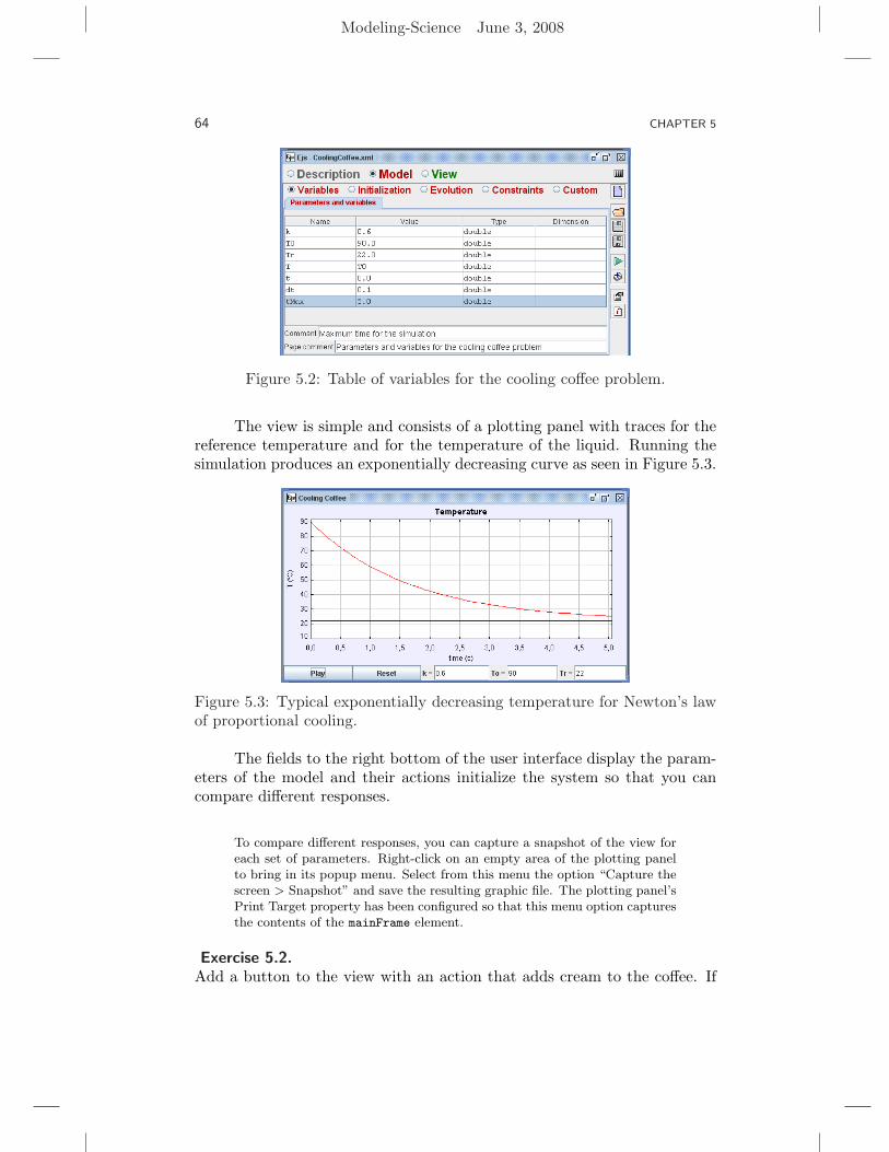
The Cooling Coffee model declares the page of variables shown inFigure 5.2. We set k = 0.6, T0 = 90, and Tr = 22 and we simulate themodel from t = 0 to t = 5. Temperature is measured in Celsius degrees andtime is measured in minutes. (What are the units for k?) We have chosena fixed discretization step dt of 0.1 minutes to compute the temperature ofthe coffee at equally spaced instants of time tk = t0 + k dt.
Enter the following code in the Evolution workpanel.
t += dt; // Increment the time
if (t>=tMax) _pause(); // stop if maximum time is exceeded
The Constraints workpanel contains a code page with the closed-formsolution (5.1.2) of the differential equation.
T = Tr + (T0-Tr)*Math.exp(-k*t); // closed-form solution
Modeling-Science June 3, 2008
64 CHAPTER 5
Figure 5.2: Table of variables for the cooling coffee problem.
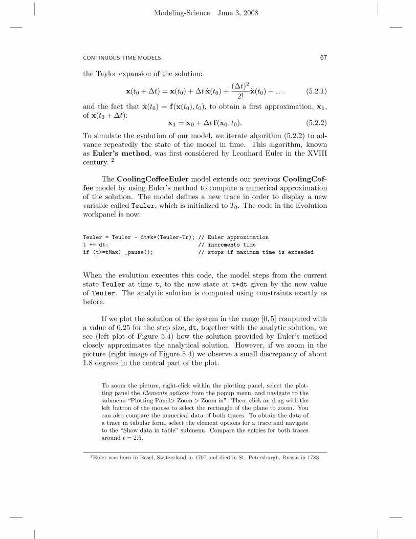
The view is simple and consists of a plotting panel with traces for thereference temperature and for the temperature of the liquid. Running thesimulation produces an exponentially decreasing curve as seen in Figure 5.3.
Figure 5.3: Typical exponentially decreasing temperature for Newton’s lawof proportional cooling.
The fields to the right bottom of the user interface display the param-eters of the model and their actions initialize the system so that you cancompare different responses.
To compare different responses, you can capture a snapshot of the view foreach set of parameters. Right-click on an empty area of the plotting panelto bring in its popup menu. Select from this menu the option “Capture thescreen > Snapshot” and save the resulting graphic file. The plotting panel’sPrint Target property has been configured so that this menu option capturesthe contents of the mainFrame element.
Exercise 5.2.Add a button to the view with an action that adds cream to the coffee. If
Modeling-Science June 3, 2008
CONTINUOUS TIME MODELS 65
the amount of time it takes to add the cream is small, the temperature ofthe coffee-cream mixture T ′ can be computed by assuming that heat lostby the coffee ∆Q− = Mc(T ′ − T ) is equal to the heat gained by the cream∆Q+ = Mc(T ′ − Tc). Assume that cream is served at Tc = 5C (41F) andthat the heat capacity c of coffee is approximately that of cream. SettingQ+ = −Q− and solving for the final temperature T ′ gives a simple equation
T ′ =MT + mTc
M + m(5.1.3)
where M ≈ 250 grams is the mass of coffee and m ≈ 25 grams is the massof cream. 2
Not all ODE problems have such a simple solution. The well-developedtheory of ordinary differential equations states that, under reasonable con-ditions on the differentiability of the expressions involved, ODEs have aunique solution for realizable initial conditions. But asserting the existenceof a solution and actually finding it are different things! Except in a fewhappy cases (see for instance [?]), ODEs are difficult or even impossible tosolve analytically. For example, the ODE
x = 3x sinx + t, (5.1.4)
has no known explicit solution.1 In cases such as this, we must resort tonumerical or graphical techniques to approximate the solutions of the equa-tions to the required level of accuracy.
When computing a particular solution of an ordinary differential equa-tion we must also providing an initial condition for the state at time t0,
x(t0) = x0. (5.1.5)
An initial condition together with a corresponding differential equation isknown as an initial value problem. Many numerical algorithms for solvinginitial value problems exist and which one to use for a given problem dependson both the cost of the computation and on the nature of the problem itself.In the following sections we describe simple methods for continuous timemodels which can be described by systems of ordinary differential equationsof the form
x(t) = f(x(t), t). (5.1.6)
We use vector notation (indicated by the use of bold font) for the state ofthe model x = {x1, x2 · · ·xn} in order to cover, later in the chapter, higher-dimensional problems. The dimension of the problem is that of the statevector. The vector function f = {f1, f2 · · · fn} expresses the rate of changeof the state as n functions of time and the state itself. A special, and very
1We will frequently follow the custom of omitting the explicit dependence on t of the statevariable x.
Modeling-Science June 3, 2008
66 CHAPTER 5
important type of differential equation is that of autonomous systems, inwhich f has no explicit dependence on time. Autonomous systems, alsocalled dynamical systems, appear frequently in the description of continuousphysical processes, such as the cooling coffee problem described above. Wediscuss the properties of these special systems in Section 5.9.
5.2 EULER METHOD
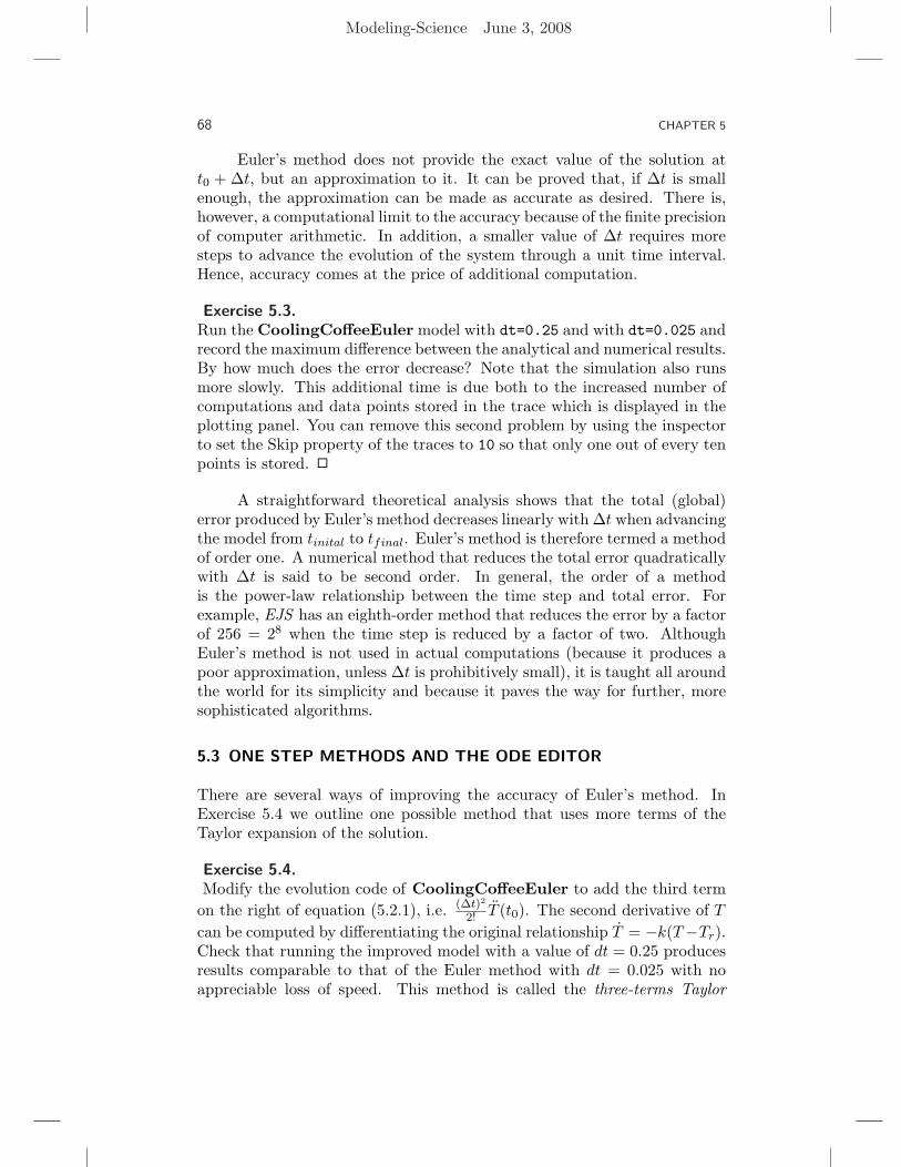
(a) Euler method and exact solutions.
(b) Zoom of a portion of the graph.
Figure 5.4: Comparison of numerical and exact solutions of the coolingcoffee problem for k = 0.6, T0 = 90, and Tr = 22 in the first five minutes.The solution computed using Euler method (the lower trace) approximatesbut does not match exactly the analytic solution. The right image shows azoomed portion of the graphs.
The standard approach to finding the numeric solution of an initialvalue problem is that of difference methods. In them, we discretize theindependent variable (usually the time) and try to compute, if only approx-imately, the value of the state at a time t0 + ∆t, for some ∆t > 0 where ∆tis called the step size. The simplest such method uses the first two terms of
Modeling-Science June 3, 2008
CONTINUOUS TIME MODELS 67
the Taylor expansion of the solution:
x(t0 + ∆t) = x(t0) + ∆t x(t0) +(∆t)2
2!x(t0) + . . . (5.2.1)
and the fact that x(t0) = f(x(t0), t0), to obtain a first approximation, x1,of x(t0 + ∆t):
x1 = x0 + ∆t f(x0, t0). (5.2.2)
To simulate the evolution of our model, we iterate algorithm (5.2.2) to ad-vance repeatedly the state of the model in time. This algorithm, knownas Euler’s method, was first considered by Leonhard Euler in the XVIIIcentury. 2
The CoolingCoffeeEuler model extends our previous CoolingCof-fee model by using Euler’s method to compute a numerical approximationof the solution. The model defines a new trace in order to display a newvariable called Teuler, which is initialized to T0. The code in the Evolutionworkpanel is now:
if (t>=tMax) _pause(); // stops if maximum time is exceeded
When the evolution executes this code, the model steps from the currentstate Teuler at time t, to the new state at t+dt given by the new valueof Teuler. The analytic solution is computed using constraints exactly asbefore.
If we plot the solution of the system in the range [0, 5] computed witha value of 0.25 for the step size, dt, together with the analytic solution, wesee (left plot of Figure 5.4) how the solution provided by Euler’s methodclosely approximates the analytical solution. However, if we zoom in thepicture (right image of Figure 5.4) we observe a small discrepancy of about1.8 degrees in the central part of the plot.
To zoom the picture, right-click within the plotting panel, select the plot-ting panel the Elements options from the popup menu, and navigate to thesubmenu “Plotting Panel> Zoom > Zoom in”. Then, click an drag with theleft button of the mouse to select the rectangle of the plane to zoom. Youcan also compare the numerical data of both traces. To obtain the data ofa trace in tabular form, select the element options for a trace and navigateto the “Show data in table” submenu. Compare the entries for both tracesaround t = 2.5.
2Euler was born in Basel, Switzerland in 1707 and died in St. Petersburgh, Russia in 1783.
Modeling-Science June 3, 2008
68 CHAPTER 5
Euler’s method does not provide the exact value of the solution att0 + ∆t, but an approximation to it. It can be proved that, if ∆t is smallenough, the approximation can be made as accurate as desired. There is,however, a computational limit to the accuracy because of the finite precisionof computer arithmetic. In addition, a smaller value of ∆t requires moresteps to advance the evolution of the system through a unit time interval.Hence, accuracy comes at the price of additional computation.
Exercise 5.3.Run the CoolingCoffeeEuler model with dt=0.25 and with dt=0.025 andrecord the maximum difference between the analytical and numerical results.By how much does the error decrease? Note that the simulation also runsmore slowly. This additional time is due both to the increased number ofcomputations and data points stored in the trace which is displayed in theplotting panel. You can remove this second problem by using the inspectorto set the Skip property of the traces to 10 so that only one out of every tenpoints is stored. 2
A straightforward theoretical analysis shows that the total (global)error produced by Euler’s method decreases linearly with ∆t when advancingthe model from tinital to tfinal. Euler’s method is therefore termed a methodof order one. A numerical method that reduces the total error quadraticallywith ∆t is said to be second order. In general, the order of a methodis the power-law relationship between the time step and total error. Forexample, EJS has an eighth-order method that reduces the error by a factorof 256 = 28 when the time step is reduced by a factor of two. AlthoughEuler’s method is not used in actual computations (because it produces apoor approximation, unless ∆t is prohibitively small), it is taught all aroundthe world for its simplicity and because it paves the way for further, moresophisticated algorithms.
5.3 ONE STEP METHODS AND THE ODE EDITOR
There are several ways of improving the accuracy of Euler’s method. InExercise 5.4 we outline one possible method that uses more terms of theTaylor expansion of the solution.
Exercise 5.4.Modify the evolution code of CoolingCoffeeEuler to add the third term
on the right of equation (5.2.1), i.e. (∆t)2
2! T (t0). The second derivative of T
can be computed by differentiating the original relationship T = −k(T−Tr).Check that running the improved model with a value of dt = 0.25 producesresults comparable to that of the Euler method with dt = 0.025 with noappreciable loss of speed. This method is called the three-terms Taylor
Modeling-Science June 3, 2008
CONTINUOUS TIME MODELS 69
method and is a second-order method because the error on a unit intervaldecreases quadratically with ∆t. 2
Although one can create more accurate numerical methods by takingsubsequent terms in the Taylor expansion, the derivatives involved becomemore and more complicated and error-prone. Moreover, the differentiationand coding effort done for one problem can not be reused for a differentODE. Over the years, mathematicians looked for numerical methods of orderhigher than one that only require the evaluation of the rate function f , andare therefore easy to reuse. Among the most popular and easy to implementfor simulation purposes are the so-called one step methods. These methodsevaluate the rate function at multiple points in the interval [t0, t0 + ∆t] andthen combine the results to provide a good approximation of the solution att0 + ∆t . Although a better approximation requires more evaluations of therate function for a single step, the extra computations pay off because thehigher accuracy implies that the step size ∆t can be increased, sometimesdramatically, reducing the total number of computations in a given inter-val of time [tinital, tfinal]. We describe some of the most popular one stepmethods in the appendix at the end of this chapter on numerical methods.
Writing a simple, fixed step size implementation of some of these meth-ods is not too difficult. However, numerical methods reach their maximumefficiency only when implemented using advanced numerical techniques thatinvolve automatically estimating the error, adapting (changing) the stepsize, and interpolating the resulting points to produce the final state. Inorder to make it easy to use such advanced solution algorithms, EJS hasa built-in ODE editor that allows you to enter the differential equations ina natural form and select the numerical method desired. Easy Java Simu-lations automatically creates Java code that uses the Open Source Physicslibrary [?] to solve the equations. We now illustrate how to use the editor toimplement a variation of the cooling coffee problem with changing outsidetemperature.
The CoolingCoffeeEditor simulation uses the ODE editor in theEvolution workpanel to implement the model of a liquid that cools in achanging outside temperature Tr(t),
T (t) = −k(T (t)− Tr(t)). (5.3.1)
Although the resulting differential equation is linear, finding the solutionrequires computing an integral which may not be analytically solvable, de-pending on the complexity of the function Tr(t). We must therefore resortto a numeric method.
Figure 5.5 shows how equation (5.3.1) is entered into the ODE editor.
Modeling-Science June 3, 2008
70 CHAPTER 5
Figure 5.5: The ODE editor of EJS used to specify the equation of thecooling coffee problem with variable reference temperature. The rate of thestate variable T on the left column is computed using the formula on theright column. Tr() is a method declared in the Custom panel of the model.
The Independent Variable property at the top of the panel is used to specifythe independent variable of the differential equation. This variable can beany continuous variable but is often the time as in the current model. TheIncrement property specifies the step size of our discretization. The centralpart of the editor contains a table showing the formula that computes therate of each of the state variables. To enter a differential equation, wedouble-click on the left column and type the corresponding state variable(T in our problem). The editor then shows the rate in the familiar dT
d t form.Alternatively, right-clicking on the state cell allows us to select the statefrom the list of model variables of double type. The rate is specified bydouble-clicking in the right column and typing the Java expression requiredfor the computation. In our case, the code is -k*(T-Tr(t)), where Tr isnow a method (function) defined in the Custom workpanel of the model withthe code:
Notice that, although time is a global variable t, the t variable in theODE editor is a local variable with possibly different values. Numericalmethods compute rates at different (intermediate) instants of time in orderto achieve better precision. For example, the fourth order Runge–Kuttamethod evaluates the rate four times when advancing the system from t0 tot0 + ∆t. Because the state variables in an ODE editor are not the globalvariables with the same name, it is crucial to follow the rule of passing the
Modeling-Science June 3, 2008
CONTINUOUS TIME MODELS 71
ODE editor’s state variables as parameters to methods in the rate columnof the editor.
Finally, the lower part of the ODE editor allows us to select one ofthe one-step methods available in EJS to solve the problem. The classicalfourth-order Runge–Kutta method chosen for this example provides an al-most perfect match with the correct solution even for large values of thestep size.
If the method selected uses an adaptive algorithm, a field will appear allowingus to enter the tolerance (or maximum local error) desired for the computa-tion. The method will then use smaller internal step sizes, if needed, to makesure that each step has an error smaller than the tolerance. A detailed expla-nation of how adaptive methods work is provided in the appendix at the endof this chapter. The Events button is used for problems with discontinuitiesin the equation and is discussed in Chapter 7.
Solving a given ODE with different methods and values of the stepsize is always recommended. The number of different algorithms used to-day accounts for the fact that no method is superior in all circumstances.Selecting an appropriate step size can help us obtain an accurate solutionwithout wasting computer power and one of the big advantages of the ODEeditor in EJS is that it makes this experimentation very easy.
Exercise 5.5.Run the CoolingCoffeeEditor model for a constant outside temperature(i.e. Tr(t) = 22.0 for all t) with different step sizes and compare the solutionobtained with the analytic one. See how large can dt be for a Runge–Kutta method. Check the order of the Runge–Kutta method to be four bycomputing how the error decreases with dt. 2
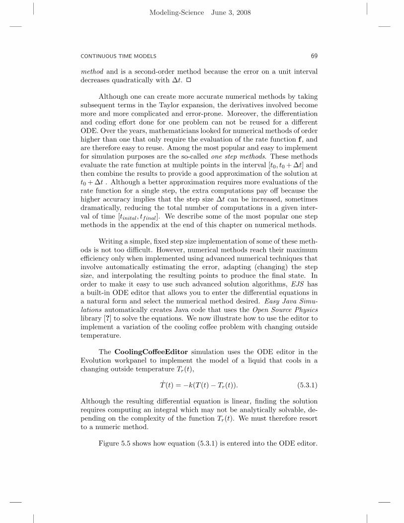
Exercise 5.6.Model the temperature of an object that is periodically heated and cooled
in a discontinuous manner. Assume that the heating-cooling cycles has afrequency f .
public double Tr (double time) {
if(Math.sin(2*Math.PI*frequency*time)<0){
return 22.0 + 10.0;
}else{
return 22.0 - 10.0;
}
}
A discontinuous Tr(t) function can confuse a numerical ODE algorithm. Aresome algorithms more successful than others in handling discontinuities? 2
Modeling-Science June 3, 2008
72 CHAPTER 5
5.4 ODE FLOW AND DIRECTION FIELDS
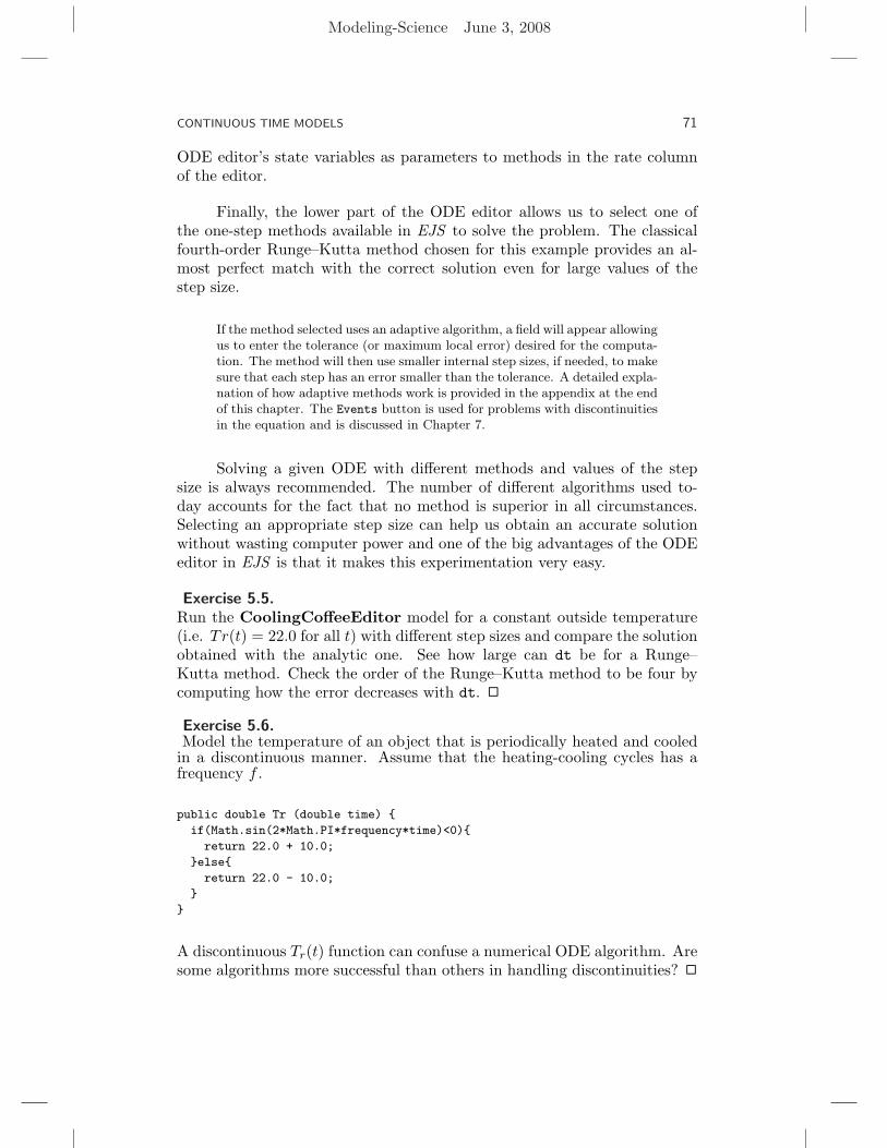
Figure 5.6: Evolution of a continuous time model for population growth.The variable which represents the population (in normalized units) changescontinuously in time with a rate which depends on its current value and onthe value of the parameters r = 1 and K = 10. The system reaches 99% ofits carrying capacity after approximately 8 time units.
Differential equations are frequently used in biology to model popula-tion dynamics. A very simple model of the evolution of the population Nstates that the species will reproduce according to the Malthusian law
N = rN, (5.4.1)
where the growth rate r is a given positive parameter. Equation (5.5.1) canbe easily solved to show an exponential increase of the population whichwould soon drive the species into overpopulation problems unless thereis infinite food and space. More sophisticated models predict exponentialgrowth for small populations but include an overcrowding term that limitsthe growth of the population due to decease and the scarcity of resources.The logistic model for a population N (expressed in suitable units) predictsthis behavior and be written as
N = rN − r
KN2 or N = rN(1− N
K) (5.4.2)
where population N(t) is a continuous function of time, r > 0 is the growthrate for small populations, and K > 0 is the ecosystem’s carrying capacity.Figure 5.6 shows that the carrying capacity is reached, starting from aninitial value of 0.5, after approximately eight time units if r = 1.00.
Although the solution for an initial value problem, such as the logisticequation, with a particular set of initial conditions is useful, we often wish tounderstand the qualitative behavior of all the possible solutions of a differ-ential equation. Even if we have an analytic solution, it may be complicatedand it may be unclear how the solution depends on the initial conditions.A better approach is to study the rate of change (flow) as a function of the
Modeling-Science June 3, 2008
CONTINUOUS TIME MODELS 73
Figure 5.7: The one-dimensional phase space flow of the logistic equation.
state variables. The Ode1DFlow model implements this visualization fora single ordinary differential equation of the form
x = f(x) . (5.4.3)
The ODE 1D Flow rate graph (Figure 5.7) shows the logistic functionf(x) = 0.1x(1 − x/10) using the generic x to represent the population.(What is the value of K?) The graph contains a draggable red circle thatrepresents the current value of x and has an arrow that shows the directionof x. If the rate is positive, the arrow is to right; if negative, the arrow is tothe left. This arrow introduces us to phase space flow, a concept that allowsus to study the geometry of a differential equation. The time developmentgraph (see Figure 5.6) displays particular solutions x(t) when the model isrun.
Exercise 5.7.Load the one-dimensional ODE flow model into EJS and run the default
(logistic) simulation. Stop the time evolution, drag the red circle past thecarrying capacity K = 10, and restart the time evolution and compare thetwo solutions. Can the circle ever move past the carrying capacity? Whatinformation that is available in the solution plot is missing from the rateplot? 2
Points where f(x) = 0 are called fixed points or equilibrium pointsbecause the rate of change is zero and the value of x remains constant.Figure 5.7 shows that the logistic equation has two fixed points. The fixedpoint at x = 0 is an unstable fixed point because solutions in its vicinityalways move (flow) away from it. The fixed point at the carrying capacityx = K is a stable fixed point because solutions in its vicinity move (flow)toward it.
Modeling-Science June 3, 2008
74 CHAPTER 5
Exercise 5.8.Use the one-dimensional ODE flow model to identify and classify the fixedpoints for x = sinx on the interval [−4π, 4π]. 2
Exercise 5.9.Use the one-dimensional ODE flow model to identify and classify the fixedpoints for x = x− x3 on the interval [−1.5, 1.5]. 2
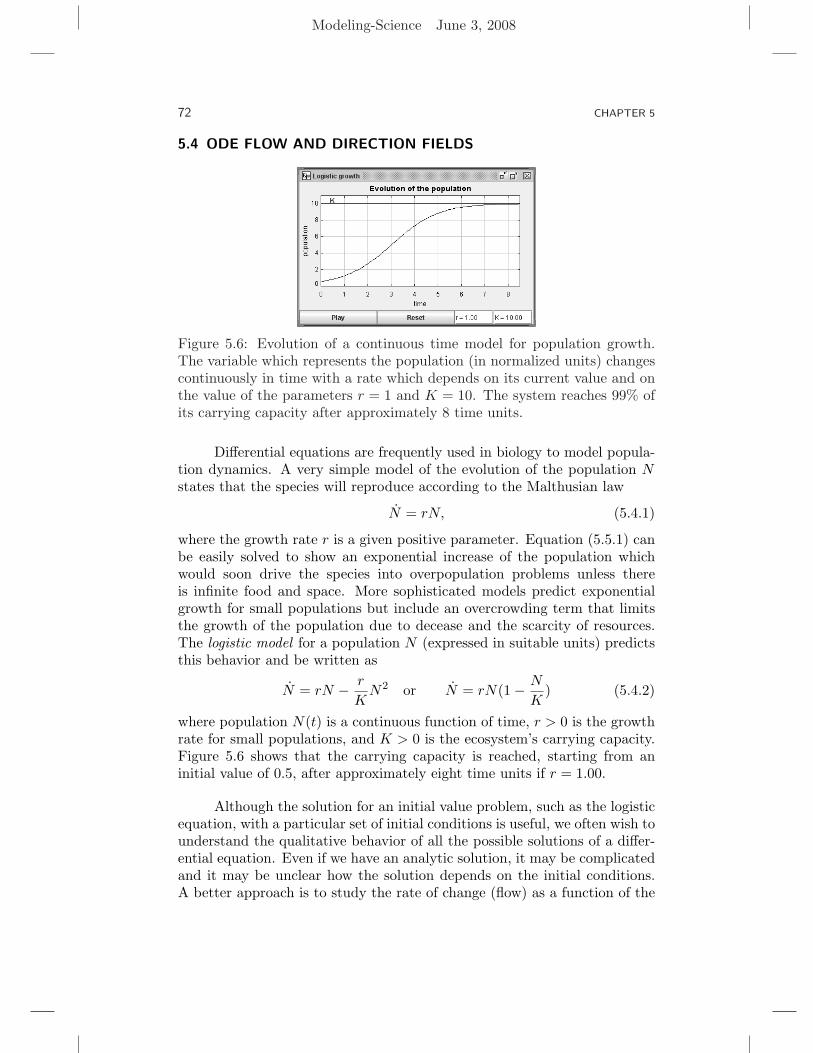
Figure 5.8: A grid of small line segments showing the direction field of theODE x = 3x sinx+ t in the range [−6, 3]× [−2, 4]. Multiple solution curveshave been computed and superimposed on the field.
A graphical technique which is commonly used for one-dimensionalequations with rate function f(x, t) that also depends on time (non-autonomousODE) is that of plotting the direction field of the ODE. This visualizationconsists of drawing a grid of line segments in the (t, x) solution plane. Eachsegment has a constant length and a slope given by f(x, t). Since the solu-tion curve obeys x(t) = f(x(t), t), the curve must be tangent to these linesegments at each of the field’s grid points. When the grid is refined, thequalitative behavior of the solution curve can frequently (but not always)be sketched. Figure 5.8 shows the direction field and a collection of solutioncurves for the ODE x = 3x sinx + t in the [−6, 3]× [−2, 4] solution plane.
The DirectionFieldPlotter model shows the direction field repre-sentation of a differential equation by superimposing ODE trajectories onan analytic vector field with components (1, f(x(t), t). The line segmentsshow the ODE rate of change and the nt and nx indexes indicate the numberof grid points in the t and x directions. The visualization uses a fixed colormap with constant length line segments as described in Section 3.8. Traceelements are used to plot the solution curves.
Modeling-Science June 3, 2008
CONTINUOUS TIME MODELS 75
Contrary to the usual way of starting the evolution using a buttonaction, this model’s evolution is started using a mouse action. Every pointwithin the plotting panel is a possible initial conditional for the differentialequation and the model generates the solution curve that passes througha point when the user clicks on that point within the panel. In order toshow the complete solution, uses separate differential equations to advanc-ing forward and backward in time from the starting time t0. Forward andbackward solutions are recorded in the solutionForward and solution-Backward Trace elements.
Note that the independent parameter t is set to zero at the start of theevolution and that this value must be added and subtracted from t0 togenerate the forward and backward solutions, respectively.
The plotting panel’s On Release action executes code that controls theanimation by invoking the following custom method:
public void compute_solution() {
// return if not left-clicking so as not to interfere with pop-up menu
if (_view.plottingPanel.getMouseButton()!=_EjsConstants.LEFT_MOUSE_BUTTON) return;
_pause(); // stop the animation
t = 0; // reset the animation time
t0 = _view.plottingPanel.getMouseX(); // get initial t
xf = xb = _view.plottingPanel.getMouseY(); // get initial x
_view.solutionForward.moveToPoint(t0+t,xf); // add first point to forward trace
_view.solutionBackward.moveToPoint(t0-t,xb);// add first point to backward trace
_play(); // start the animation
}
We use the getMouseButton() method to identify the mouse button thatwas released so as not to interfere with the plotting panel’s pop-up menu. Ifthe left button is pressed, the code stops the animation and reads the mousecoordinates to initialize the model’s state variables. The code then addsinitial values to the Trace elements that record the forward and backwardsolutions and starts the animation. The Evolution workpanel advances theboth xf and xb. The evolution is stopped if the solution can no longer beseen within the plotting panel using a constraint that performs the followingbounds check.
_pause(); // stop if both solutions are out of bounds
Modeling-Science June 3, 2008
76 CHAPTER 5
The Direction Field model is a good example of how to start andstop the evolution from within a model and we encourage you to study itcarefully.
Exercise 5.10.Predict (sketch the direction field for logistic model. Pay particular attentionto the direction field at the fixed points. Test your prediction using theDirectionFieldPlotter model. The logistic model is autonomous. Howdoes this affect the direction field? 2
Exercise 5.11.Use the DirectionField simulation to draw the direction fields for the
following ODEs in the given regions of the plane. Sketch the solution curvesbefore clicking within the simulation to compute the solution.
• x = −k(x − Tr), for k = 0.03 and Tr = 22 in [0, 5] × [10, 90]. (Thecooling coffee problem.)
• x = (1− t)x− t, in [−2, 4]× [−4, 2].
• x = (x− 3)(x + 1)/(1 + x2), in [−5, 5]× [−3, 5].
• x = −x cos t + sin t, in [−10, 10]× [−10, 10].
• x = 3t2/(3x2 − 4), in [−2, 2]× [−2, 2].
2
The last equation in Exercise 5.11 shows that numeric methods are notinfallible. The solver fails to find the right solutions at the turning points(as indicated by vertical field segments). The reason is that the ODE isincorrectly defined for points in the vertical lines x = ±
√4/3.
Exercise 5.12.Change the solver of the ODE editor to the adaptive method Runge-Kutta-Fehlberg5(4) and test it with the last of the equations in Exercise 5.11. See that theEJS console prints an non-convergence warning when the trajectories reachthe line x = ±
√4/3. Fixed step methods simply ignore the problem and
try to step forward at any cost (and provide wrong solutions). 2
5.5 PREDATOR AND PREY
Higher dimensional differential equations appear naturally in continuousmodels of real-life processes. One of the nicest examples of a two-dimensional
Modeling-Science June 3, 2008
CONTINUOUS TIME MODELS 77
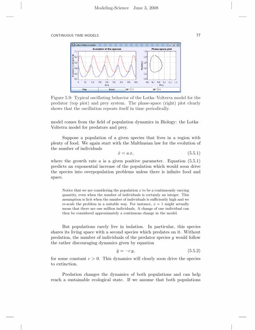
Figure 5.9: Typical oscillating behavior of the Lotka–Volterra model for thepredator (top plot) and prey system. The phase-space (right) plot clearlyshows that the oscillation repeats itself in time periodically.
model comes from the field of population dynamics in Biology: the Lotka–Volterra model for predators and prey.
Suppose a population of a given species that lives in a region withplenty of food. We again start with the Malthusian law for the evolution ofthe number of individuals
x = a x, (5.5.1)
where the growth rate a is a given positive parameter. Equation (5.5.1)predicts an exponential increase of the population which would soon drivethe species into overpopulation problems unless there is infinite food andspace.
Notice that we are considering the population x to be a continuously varyingquantity, even when the number of individuals is certainly an integer. Thisassumption is licit when the number of individuals is sufficiently high and were-scale the problem in a suitable way. For instance, x = 1 might actuallymean that there are one million individuals. A change of one individual canthen be considered approximately a continuous change in the model.
But populations rarely live in isolation. In particular, this speciesshares its living space with a second species which predates on it. Withoutpredation, the number of individuals of the predator species y would followthe rather discouraging dynamics given by equation
y = −c y, (5.5.2)
for some constant c > 0. This dynamics will clearly soon drive the speciesto extinction.
Predation changes the dynamics of both populations and can helpreach a sustainable ecological state. If we assume that both populations
Modeling-Science June 3, 2008
78 CHAPTER 5
are constantly mixed in space, then predation takes place continuously andturns the dynamics into a coupled two-dimensional system given by
x = a x− b xy,
y = −c y + d xy.(5.5.3)
The positive constants b and d account for the predation rate of the encoun-ters between individuals of both species, and the increase in the reproductionrate of the predators produced by the nutritive value of the predation, re-spectively. This system of ODEs is called the Lotka–Volterra model forpredators and prey.
Different examples of predator-prey systems have been considered inreal applications. Historically, the first Lotka–Volterra model was appliedby the Italian mathematician Vito Volterra 3 to explain why the percentageof the catch of two different categories of fishes in the Mediterranean Seachanged during World War I. The predator group of species were selachians(sharks, skates, rays, . . . ) which prey on other, more desirable food fishharvested by ships from the port of Fiume, Italy, during the years 1914–1923. A very nice historical and theoretical note of this study can be foundin [?] and [?].
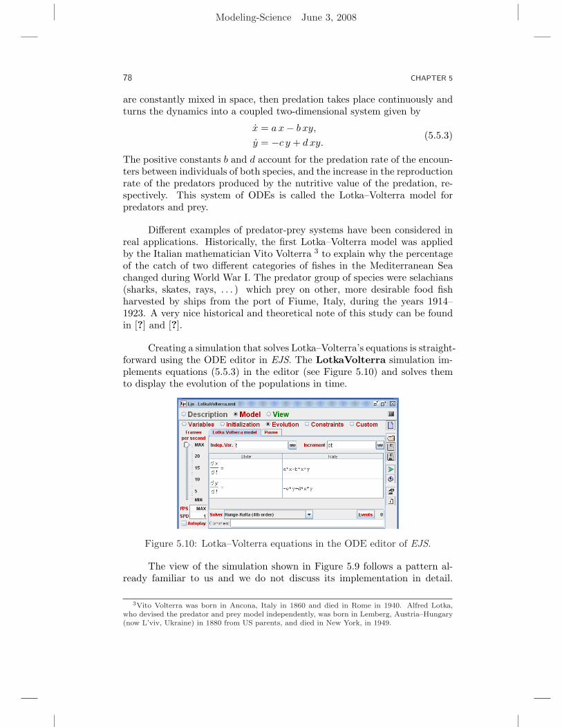
Creating a simulation that solves Lotka–Volterra’s equations is straight-forward using the ODE editor in EJS. The LotkaVolterra simulation im-plements equations (5.5.3) in the editor (see Figure 5.10) and solves themto display the evolution of the populations in time.
Figure 5.10: Lotka–Volterra equations in the ODE editor of EJS.
The view of the simulation shown in Figure 5.9 follows a pattern al-ready familiar to us and we do not discuss its implementation in detail.
3Vito Volterra was born in Ancona, Italy in 1860 and died in Rome in 1940. Alfred Lotka,who devised the predator and prey model independently, was born in Lemberg, Austria–Hungary(now L’viv, Ukraine) in 1880 from US parents, and died in New York, in 1949.
Modeling-Science June 3, 2008
CONTINUOUS TIME MODELS 79
Notice however that we are not displaying the solution curves of the sys-tem. The solution would be a three-dimensional curve given by points ofthe form (x, y, t). Instead, the left panel shows the component graphs ofthe solution, given by points of the form (x(t), t) and (y(t), t), and the rightpanel shows the trajectory of the solution in phase-space, given by pointsof the form (x, y). This display is similar to what we did in the mass andspring example of Chapter 2.
The component graphs provide information of how the population ofeach species changes in time and is very close to how fishermen would an-notate the populations of fish in a time register. We can see the alternateextrema of both species. The ups an downs of the predators follow closelythose of the prey, as one would expect.
The phase-space (also called state-space) plot is a mathematical so-phistication consisting in projecting the three-dimensional solution curveinto the plane span by the state coordinates. Although this projection loosesthe time information (we cannot tell when the trajectory passes through agiven (x, y) point), it provides important information which is not easilyappreciated in the component graphs or the three-dimensional curve. Forinstance, the right view of Figure 5.9 immediately suggests that trajecto-ries are periodic, i.e. they repeat themselves periodically in time. Volterraproved mathematically that all phase-space trajectories of equations (5.5.3)are periodic. The period of the trajectories, i.e. the minimum time for whichthey repeat themselves, varies slightly depending on the trajectory. Thesole exceptions are the trajectories that start at points (0, 0) and (c/d, a/b),which are constant. Constant trajectories are known as equilibrium solutionsor stationary states.
Additional information can be obtained from phase-space plots forautonomous systems. (The Lotka–Volterra model is an autonomous systembecause the rates of x and y do not depend on time.) Trajectories in phase-space of autonomous systems can’t cross each other, which limits the kindof possible behavior for trajectories. Also, if a trajectory of an autonomoussystem passes twice through a given point, it becomes periodic. Autonomoussystems are discussed in more detail in Section ??.
Exercise 5.13. Volterra’s law of averages.Volterra also proved analytically that, despite having different periods, theaverage predator population over a period is precisely c/d and the averageof the prey population a/b. The averages are given by the integrals
x =1T
∫ T
0x(t) dt, y =
1T
∫ T
0y(t) dt, (5.5.4)
Modeling-Science June 3, 2008
80 CHAPTER 5
where T is the period of the particular trajectory considered. Show this factby computing numerically this average. [Hint: Modify simulation Lotka-Volterra so that, given initial conditions (x0, y0), it counts the accumulatedpopulation (times the step size) at each integration step until the trajectorypasses again the line y = y0 from below. Divide then the counter by thetime elapsed and compare to the value predicted by Volterra.] 2
Exercise 5.14. Sensitivity to initial conditions in modified Lotka–Volterra systemsSuppose the reproduction rate of the prey undergoes periodic changes (ac-cording to seasons, say). Change the system so that a = a1 + a2 ∗ cos(f t),where a1 denotes a fixed rate and a2 and f define a periodic fluctuation.Show that the system now can be very sensitive to initial conditions. Use forinstance a1 = 0.172, a2 = 0.25, and f = 0.3. Plot the trajectory with initialconditions x0 = 0.46501, and y0 = 0.40811 until t = 800 and then compareit with the trajectory which starts at the same x0 but with y0 = 0.40810(a difference of only 10−5!). Sensitivity to initial conditions, together witherratic behavior are footprints of chaos. 2
5.6 NEWTONIAN MECHANICS
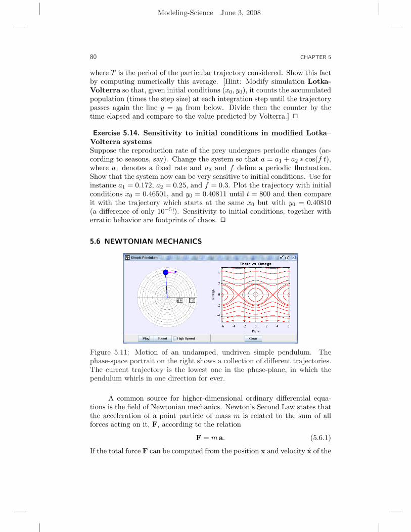
Figure 5.11: Motion of an undamped, undriven simple pendulum. Thephase-space portrait on the right shows a collection of different trajectories.The current trajectory is the lowest one in the phase-plane, in which thependulum whirls in one direction for ever.
A common source for higher-dimensional ordinary differential equa-tions is the field of Newtonian mechanics. Newton’s Second Law states thatthe acceleration of a point particle of mass m is related to the sum of allforces acting on it, F, according to the relation
F = ma. (5.6.1)
If the total force F can be computed from the position x and velocity x of the
Modeling-Science June 3, 2008
CONTINUOUS TIME MODELS 81
particle and the time t, equation (5.6.1) expresses a differential relationshipof the form
x =1m
F(x, ˙x, t). (5.6.2)
This equation is a second order differential vector equation with the di-mension of the position variable x. Second and higher order problems can beconverted into ordinary (first order) differential equations of the form (5.1.6)introducing additional variables for the derivatives of the state vector. Thus,equation (5.6.2) for a particle with coordinates x = (x1, x2, . . . , xn) can berewritten in the desired form by introducing a new state vector
x′ = (x1, v1, x2, v2, . . . , xn, vn) (5.6.3)
where vi = xi. Notice that this procedure doubles the dimension of thestate vector so we have twice as many differential equations to solve. But itmakes the problem accessible using the numerical methods for the solutionof first-order equations presented in this chapter.
We saw a first example of a mechanical system describing the motionof a mass and spring in Chapter 2. That motion displayed the characteristicsof a linear oscillator. We consider now the simplest example of a non-linearoscillator. A simple pendulum is a physical abstraction consisting of a pointmass m which oscillates at the end of a rigid massless rod of fixed length L.
Massless rods and point masses are abstractions that do not exist. However,a dense small sphere at the end of a light thin rod is a good approximate forthe idealized pendulum.
When the pendulum is at rest, it will hang vertically from the pivotpoint. When displaced from the vertical and released from rest (with noinitial velocity), the pendulum will oscillate in the plane which contains thevertical line through the pivot point and the initial position. This restrictionconverts a problem in space into a problem in the plane. Because of therigidity of the rod, the motion of the mass is restricted to a circumference.Polar coordinates (r, θ) are therefore more appropriate for this problem thanthe usual cartesian coordinates (x, y). The radial component r is fixed andequal to the length of the rod L. The interesting dynamics is related to thechange of the angular coordinate θ.
Newton’s Law for planar rotation states that the angular accelerationθ of an object is proportional to the torque τ applied to that object,
τ = I θ. (5.6.4)
The constant of proportionality I is known as the moment of inertia and
Modeling-Science June 3, 2008
82 CHAPTER 5
can be shown to be I = mL2 for a point mass that is at a distance L fromthe point of rotation. Applying Newton’s Second Law for rotation to thependulum leads to the following second-order differential equation
θ = −g
`sin(θ). (5.6.5)
Following the procedure indicated above, we introduce the new vari-able given by angular velocity ω = θ to turn this second-order equation intoan equivalent first order system
θ = ω
ω = −g
`sin(θ).
(5.6.6)
This is the first order system of ODEs for the (undamped, undriven) simplependulum. Additional terms must be introduced when the system includesfrictional or driving forces.
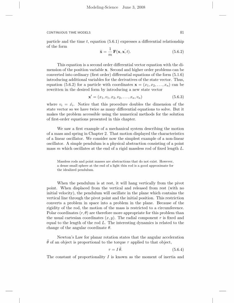
The SimplePendulum model implements equations (5.6.6) using theODE editor of EJS and shows the evolution of the pendulum using botha realistic representation of the motion of the pendulum and a phase-spacediagram. The model declares three separate pages of variables for organiza-tional reasons. See Figure 5.12.
Figure 5.12: Three different tables help organize the variables of the simplependulum model. Pages of variables are processed from left to right.
All variables in these tables have global visibility irrespective of thepage in which they have been declared. A single exception is that variablescan be used in the Value column of other variables only if they have beendeclared earlier in the same table or in a previous page of variables. Pagesof variables are processed from left to right.
The ODE editor is used to state and solve the differential equations (5.6.6).
Modeling-Science June 3, 2008
CONTINUOUS TIME MODELS 83
Figure 5.12 shows we have chosen an adaptive algorithm with a tolerance of10−5 to compute the solution.
Figure 5.13: First order system of differential equations equivalent to thesecond order problem θ = − g
L sin(θ).
Because the equations of motion are solved in polar coordinates, themodel includes a page of constraints with the following code to convert frompolar to cartesian coordinates.
x= L*Math.sin(theta);
y = -L*Math.cos(theta);
vx = omega*L*Math.cos(theta);
vy = omega*L*Math.sin(theta);
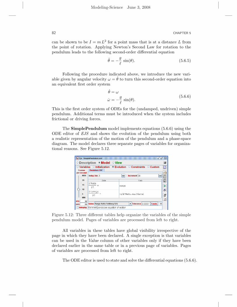
These cartesian coordinates are used to position the bob and its ve-locity vector in the left plotting panel of Figure 5.11. This plotting paneldisplays (for aesthetic reasons, mainly) polar axes according to the valueof its Axis Type property. The property inspector displayed in Figure 5.14shows the location of the bob is given using the constrained x and y coordi-nates.
The polar-cartesian dichotomy forces us to provide an action for theview element which displays the bob. When the user drags the bob to a newposition, the action code computes the correct value of the theta angle.
theta = Math.atan2(x,-y);
// length is constant
omega = 0.0;
t = 0.0;
The Math.atan2(a,b) method computes the angle subtended by the givencoordinates in the [0, 2π] interval which is used as the new value of theta.
Modeling-Science June 3, 2008
84 CHAPTER 5
Figure 5.14: Property inspector for the bob view element. Because its posi-tion is given by cartesian coordinates, action code is required to update themodel polar coordinates.
The action code also resets the time and sets the angular velocity to zeroso that the motion starts from rest. Because L is not changed, constraints(which will be called automatically by EJS after the action is executed) willcorrect the values of the x and y coordinates so that the bob remains at thecorrect distance from the pivot.
The right plotting panel of the view of this simulation is preparedto display a phase-portrait of the simple pendulum. A phase-portrait isa visualization of a moderately large collection of different trajectories inphase-space, and provides a good deal of information of the qualitative be-havior of the solutions of the system. The user can click on any point inphase-space and obtain the trajectory through that point.
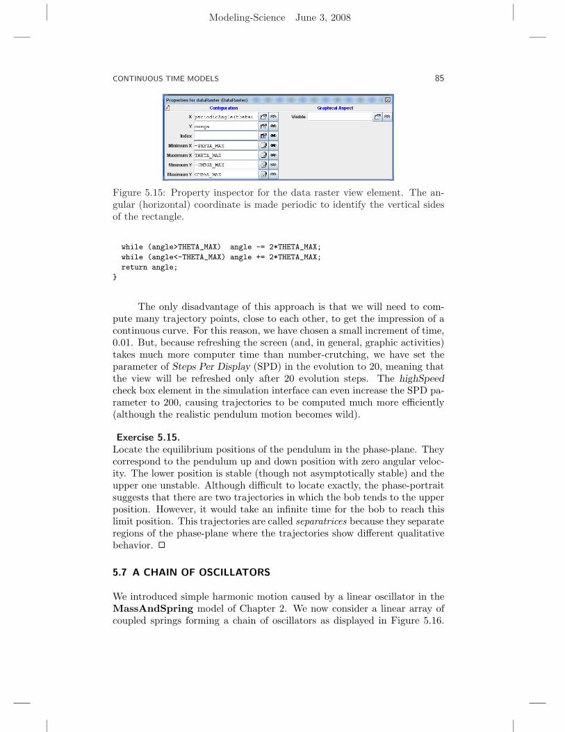
We have chosen to display the trajectories in the phase-portrait asa collection of separate points, rather than using a connected trace. Thereason is that displaying a complete phase-portrait such as the one shownin Figure 5.11 requires plotting a large number of points. Although a singletrace can also display several trajectories, too many points can make thecomputer slower and even run out of memory. The DataRaster elementwe used instead accepts individual points within prescribed minimum andmaximum coordinates and prepares an off-screen bitmap image which itdumps to the screen when the view is refreshed. The memory usage isminimal and the drawing very fast. Points are added to the data raster bylinking its X and Y properties with the values of theta and omega, as shownin Figure 5.15.
We make the phase-space appear periodic in the angular dimension byidentifying points in the vertical sides of the rectangle through the peridoicAnglecustom method.
public double periodicAngle(double angle) {
Modeling-Science June 3, 2008
CONTINUOUS TIME MODELS 85
Figure 5.15: Property inspector for the data raster view element. The an-gular (horizontal) coordinate is made periodic to identify the vertical sidesof the rectangle.
while (angle>THETA_MAX) angle -= 2*THETA_MAX;
while (angle<-THETA_MAX) angle += 2*THETA_MAX;
return angle;
}
The only disadvantage of this approach is that we will need to com-pute many trajectory points, close to each other, to get the impression of acontinuous curve. For this reason, we have chosen a small increment of time,0.01. But, because refreshing the screen (and, in general, graphic activities)takes much more computer time than number-crutching, we have set theparameter of Steps Per Display (SPD) in the evolution to 20, meaning thatthe view will be refreshed only after 20 evolution steps. The highSpeedcheck box element in the simulation interface can even increase the SPD pa-rameter to 200, causing trajectories to be computed much more efficiently(although the realistic pendulum motion becomes wild).
Exercise 5.15.Locate the equilibrium positions of the pendulum in the phase-plane. Theycorrespond to the pendulum up and down position with zero angular veloc-ity. The lower position is stable (though not asymptotically stable) and theupper one unstable. Although difficult to locate exactly, the phase-portraitsuggests that there are two trajectories in which the bob tends to the upperposition. However, it would take an infinite time for the bob to reach thislimit position. This trajectories are called separatrices because they separateregions of the phase-plane where the trajectories show different qualitativebehavior. 2
5.7 A CHAIN OF OSCILLATORS
We introduced simple harmonic motion caused by a linear oscillator in theMassAndSpring model of Chapter 2. We now consider a linear array ofcoupled springs forming a chain of oscillators as displayed in Figure 5.16.
Modeling-Science June 3, 2008
86 CHAPTER 5
Figure 5.16: A chain of coupled linear oscillators modeled with EJS. Theconfiguration displayed here corresponds to a normal mode where everyparticle moves sinusoidally with the same frequency.
This model can be used to study the propagation of waves in a continuousmedium and the vibrational modes of a crystalline lattice.
The OscillatorChain model contains 31 coupled oscillators equallyspaced within the interval [0, 2π] and with fixed ends. Let yi = y(xi, t)represent the displacement of a particle with horizontal position xi alongthe oscillator chain. Because it is assumed that the particles do not move inthe x-direction, we need only consider forces in the vertical direction. Theforce Fi on the i-th particle depends on the relative vertical displacementbetween that particle and its nearest neighbors and can be written as
Fi = −k[(yi+1 − yi)− (yi − yi−1)]. (5.7.1)
where the Hooke’s Law k constant is the same for all springs.
The main page of variables of this model, displayed in Figure 5.17,declares one-dimensional arrays for the dynamic variables x, y and vy.
Figure 5.17: Dynamic variables for the oscillator chain. Arrays of n lengthare used for the coordinates and velocities of the particles.
Declaring an array is certainly appropriate for this problem due to the
Modeling-Science June 3, 2008
CONTINUOUS TIME MODELS 87
large number of particles involved. The initialization of the horizontal andvertical positions of the masses, x and y, requires the following code in aninitialization page of the model.
_pause();
t = 0;
double x0 = 0;
for(int i=0; i<n; i++) {
x[i] = x0;
y[i] = _view.function.evaluate(x0);
v[i] = 0;
x0 += dx;
}
This code distributes the masses according to an initial pulse given by theexpression introduced by the user in the Function element of the view.
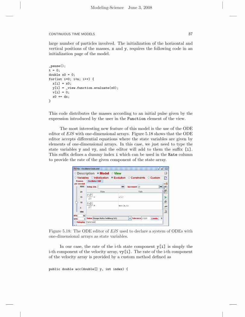
The most interesting new feature of this model is the use of the ODEeditor of EJS with one-dimensional arrays. Figure 5.18 shows that the ODEeditor accepts differential equations where the state variables are given byelements of one-dimensional arrays. In this case, we just need to type thestate variables y and vy, and the editor will add to them the suffix [i].This suffix defines a dummy index i which can be used in the Rate columnto provide the rate of the given component of the state array.
Figure 5.18: The ODE editor of EJS used to declare a system of ODEs withone-dimensional arrays as state variables.
In our case, the rate of the i-th state component y[i] is simply thei-th component of the velocity array, vy[i]. The rate of the i-th componentof the velocity array is provided by a custom method defined as
public double acc(double[] y, int index) {
Modeling-Science June 3, 2008
88 CHAPTER 5
if (index==0 || index==n-1) return 0;
else return k*(y[index-1]+y[index+1]-2*y[index]);
}
which corresponds to equation (5.7.1) (for unit masses). The fixed end pointsof the chain have zero acceleration. Finally, a page of constraints computesthe lengths of the springs which will be used for the visualization.
The view of the simulation uses sets of drawable elements to displaythe n particles and n-1 springs which form the chain. Of particular interestis the On Drag action property of the particles element. The code
double xp=0;
for (int i=0; i<n; i++) {
x[i] = xp;
xp += dx;
}
_resetSolvers();
reinitializes the x array to equidistant values to counteract the possibilitythat the user drags the masses horizontally. The resetSolvers() prede-fined method of EJS is required only in case we plan to use a numeric solverfor the ODE which uses interpolation. Using an interpolator solver whenthere is a high number of equations involved may improve performance. In-terpolation solvers keep an internal copy of the ODE state that they use in-telligently to optimize the performance of the solver. The resetSolvers()method must be called whenever the user changes the state of the simulationso that interpolators can update their internal state to match that of thesystem. Solvers which use interpolation are clearly marked in the Solvercombo box.
One way of understanding a lattice of N coupled oscillators of length Land mass M is to study the motion of its normal modes. A normal mode isa special configuration (state) where every particle moves sinusoidally withthe same frequency. The m-th mode Φm of the oscillator chain of length Lis
Φm(x) = sinmπ x
L. (5.7.2)
The system stays in a single mode and every particle oscillates with constantangular frequency ωm if the oscillator chain is initialized in a single mode.
ωm =4k
Msin
m π
2N). (5.7.3)
Modeling-Science June 3, 2008
CONTINUOUS TIME MODELS 89
Normal modes are important because an arbitrary initial configuration canbe expressed as sum of normal modes.
Exercise 5.16.Run the OscillatorChain model and experiment with different normalmodes. The m-th normal mode of this system can be observed by enteringf(x) = sin(mx/2) as the initial displacement. Do all particles oscillate withthe same frequency in given normal mode? Do all normal modes have thesame oscillatory frequency? Are there a finite or an infinite number of nor-mal modes? (That is, what happens to the oscillator chain as m increases.)2
Wave propagation can be studied by entering a localized pulse or bysetting the initial displacement to zero and dragging oscillators to form awave packet. An interesting and important feature of the OscillatorChainmodel is that the speed of a sinusoidal wave along the oscillator array de-pends on its wavelength. This causes a wave packet to disperse (changeshape) and imposes a maximum frequency of oscillation (cutoff frequency)as is observed in actual crystals.
Exercise 5.17. Dispersion exercise here.2
5.8 A MINI SOLAR SYSTEM*
Figure 5.19: An n-body problem with approximate data from the Sun,Venus, Earth and Mars. The right, geocentric view clearly shows the appar-ent retrograde motion historically observed on Mars.
The implementation of the model of the previous section showed anadvanced feature of the ODE editor which helps declare differential equa-
Modeling-Science June 3, 2008
90 CHAPTER 5
tions for systems of very high dimensions. In the case in which the variablesare not very much interrelated, i.e. the rate of a state variable depends onlyin a few other states, differentiating array elements independently (as wedid) can appropriately solve the problem. In other situations, this approachcan be rather inefficient and we demonstrate a more efficient approach inthis section.
Exercise 5.18.The OscillatorArray model computes the acceleration of the oscillators us-ing a single custom method named double[] acc(double[] y) that takesan array as input and returns an array containing accelerations. Comparethe implementation of the custom methods in the OscillatorChain andOscillatorArray models and also note the very slight difference in theODE editors. Which custom method is easier to code? Which is easier tounderstand? Which is more efficient? Give reasons for your answers. 2
Consider a small solar system in which three planets with approxi-mately similar masses orbit a central, more massive star following orbitswhich are in the same plane. Newton’s Universal Gravitation Law statesthat every two (spherical and with uniform density) bodies attract them-selves with a force given by
Fij = −GMiMj
‖ri − rj‖2
ri − rj
‖ri − rj‖ . (5.8.1)
Fij is the force exerted on the body i by the body j. G is the UniversalGravitational constant 6.67428 × 10 > −11 m3Kg−1s−2, the M ’s are themasses of the bodies, and the r’s the position vectors of the centers of thebodies. The minus sign in equation (5.8.1) makes this an attractive force,directed along the relative position vector ri − rj .
Implementing the resulting system of equations using an approachsimilar to that of Section 5.7 is possible but very inefficient. In the first place,notice that computing the acceleration of a given body means computing thesum of the forces exerted by all other bodies. However, because Fij = −Fji
(Newton’s Third Law), we are bound to compute each force twice. Also,computing separately the x and y components of any of these forces willmake us repeat the costly computation of ‖ri − rj‖.
To help us improve the efficiency in cases like this, the ODE editorof EJS allows us to specify all the states of the system in a single one-dimensional array, which is then differentiated as a whole. The SolarSys-tem model displayed in Figure 5.19 creates a one-dimensional state arraywith as many as 4*nBodies entries. Every four entries of this array willcontain the values of x, y, vx, and vy for each of the bodies. Figure 5.20
Modeling-Science June 3, 2008
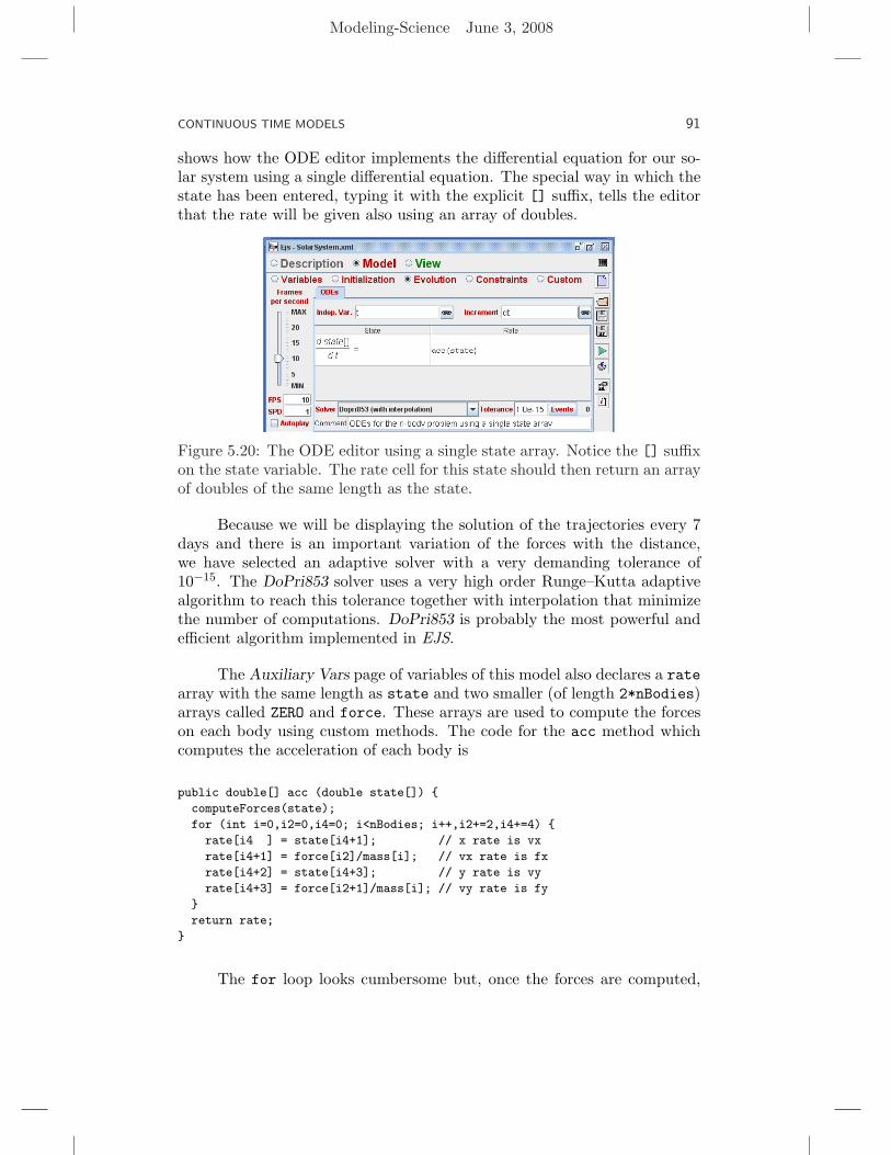
CONTINUOUS TIME MODELS 91
shows how the ODE editor implements the differential equation for our so-lar system using a single differential equation. The special way in which thestate has been entered, typing it with the explicit [] suffix, tells the editorthat the rate will be given also using an array of doubles.
Figure 5.20: The ODE editor using a single state array. Notice the [] suffixon the state variable. The rate cell for this state should then return an arrayof doubles of the same length as the state.
Because we will be displaying the solution of the trajectories every 7days and there is an important variation of the forces with the distance,we have selected an adaptive solver with a very demanding tolerance of10−15. The DoPri853 solver uses a very high order Runge–Kutta adaptivealgorithm to reach this tolerance together with interpolation that minimizethe number of computations. DoPri853 is probably the most powerful andefficient algorithm implemented in EJS.
The Auxiliary Vars page of variables of this model also declares a ratearray with the same length as state and two smaller (of length 2*nBodies)arrays called ZERO and force. These arrays are used to compute the forceson each body using custom methods. The code for the acc method whichcomputes the acceleration of each body is
public double[] acc (double state[]) {
computeForces(state);
for (int i=0,i2=0,i4=0; i<nBodies; i++,i2+=2,i4+=4) {
rate[i4 ] = state[i4+1]; // x rate is vx
rate[i4+1] = force[i2]/mass[i]; // vx rate is fx
rate[i4+2] = state[i4+3]; // y rate is vy
rate[i4+3] = force[i2+1]/mass[i]; // vy rate is fy
}
return rate;
}
The for loop looks cumbersome but, once the forces are computed,
Modeling-Science June 3, 2008
92 CHAPTER 5
it just uses the (x,vx,y,vy) structure of the state array to fill the corre-sponding rate entries. The model derived from equation (5.8.1) is reallyimplemented in the computeForces() method.
public void computeForces(double[] state) {
System.arraycopy(ZEROS,0,force,0,force.length); // clears the force array
for(int i=0,i2=0,i4=0; i<nBodies; i++,i2+=2,i4+=4) { // for each body
for(int j=i+1,j2=2*j,j4=4*j; j<nBodies; j++,j2+=2,j4+=4) { // against other bodies
double dx = state[i4 ] - state[j4 ];
double dy = state[i4+2] - state[j4+2];
double r2=dx*dx+dy*dy;
double r3=r2*Math.sqrt(r2);
double fx=G*mass[i]*mass[j]*dx/r3;
double fy=G*mass[i]*mass[j]*dy/r3;
force[i2] -= fx; // force array alternates fx and fy
force[i2+1] -= fy;
force[j2] += fx;
force[j2+1] += fy;
}
}
}
Because the second loop starts from j=i+1, each force is only computedonce, using Newton’s Third Law to update simultaneously the forces onbodies i and j. Notice also the x and y components of each force arederived with the same computational effort.
See how we used the ZEROS array (which is a constant array of zeros) to cleanthe contents of the force array. The use of the System.arraycopy methodprovided by Java is more efficient than a loop of the formfor(int i=0; i<force.length; i++) force[i] = 0.0;
The simulation displayed in Figure 5.19 shows the trajectories of amini solar system composed of the Sun, Venus, the Earth, and Mars usingreal astronomical data taken from [?]. The data, indicated in an initial-ization page, is appropriately converted so that the unit of length is oneAstronomical Unit (1AU = 149.597 × 10⁹ meters), the unit of mass is themass of the Earth (5.9736× 1024 Kilograms), and the unit of time one day.A second initialization page computes the center of masses and makes it the(inertial) reference frame. This change of frame is helpful for situations inwhich there is not a very massive body which won’t barely move and canbe used as the center of the reference frame.
The view uses the ParticleSet and TraceSet elements to displaythe motion of the bodies both in a frame located in the center of mass
Modeling-Science June 3, 2008
CONTINUOUS TIME MODELS 93
and in a geocentric view. This second view allows us to see the apparentretrograde motion of the planets as seen from the Earth. See Figure 5.19.In order to give the bodies different colors we defined an array of variablesof Object type and initialized the elements in this array using the Java classjava.awt.Color (see Appendix ??). The particles are also given differentsizes (although not to scale).
Exercise 5.19.The Solar System initialization page contains also data for Jupiter and Sat-urn. Change the value of the nBodies variable to 6 to see them. 2
Exercise 5.20.This exercise shows that if the Sun wouldn’t have been so massive as com-pared to its planets, the motion of the Earth (and therefore life on it) wouldhave followed a much more different fate. Make Mars much more massive(as much as one-tenth the mass of the Sun) and see how the orbits of theinner planets become erratic. 2
Exercise 5.21.Simulate the orbit of a planet orbiting a binary star. A binary star isactually a set of two stars with similar masses orbiting around each other.Make Mars as massive as the Sun and locate Venus and the Earth away fromboth. Show that orbits close to the binary star are very unstable (eventuallyeven escaping from the system) while those far enough from the center ofmasses of the binary stars approximate elliptical trajectories.
Disable the Center of Masses initialization page (right-click on its taband select the entry Enable/Disable this page) and see how the whole systemslowly drifts up making the description of motion even more complicated.Choosing the right reference frame is frequently an important decision. 2
5.9 DIRECTION FIELDS OF PLANAR AUTONOMOUS SYSTEMS*
[Note to reader: The 3D Vector Field element used in this section is prelim-inary. The 3D code here will likely change in the next release of Easy JavaSimulations.]
The Lotka–Volterra model is an example in which the typical qualita-tive behavior of all trajectories is more interesting than a particular solutionwith given initial conditions. Providing initial conditions for the numberof different fishes in the Mediterranean Sea, for instance, can only be donethrough statistical (approximate) means. Because the model is non-linear,we need to use numerical and graphical techniques to study the qualitativebehavior of solutions.
Modeling-Science June 3, 2008
94 CHAPTER 5
It is possible to define a direction field for two-dimensional systems inwhich a segment is drawn for each point in (x, y, t)-space, similarly to whatwe did for one-dimensional systems in Section 5.4. However, the plot willnow be three-dimensional and difficult to apprehend. For two-dimensional,autonomous systems of the form
x = f1(x, y)y = f2(x, y),
(5.9.1)
it is more common to plot a map similar to a phase-space. We then draw asegment at each point of a grid in the (x, y)-plane, according to the directiongiven by the vector (f(t, x, y), g(t, x, y)). This plot is also called a directionfield (although it is different from the direction field introduced previously)because it is the field for the one-dimensional ODE obtained dividing theequations in (5.9.1):
d y
d x=
f2(x, y)f1(x, y)
. (5.9.2)
(Notice that in this new problem, the independent variable is now x.)
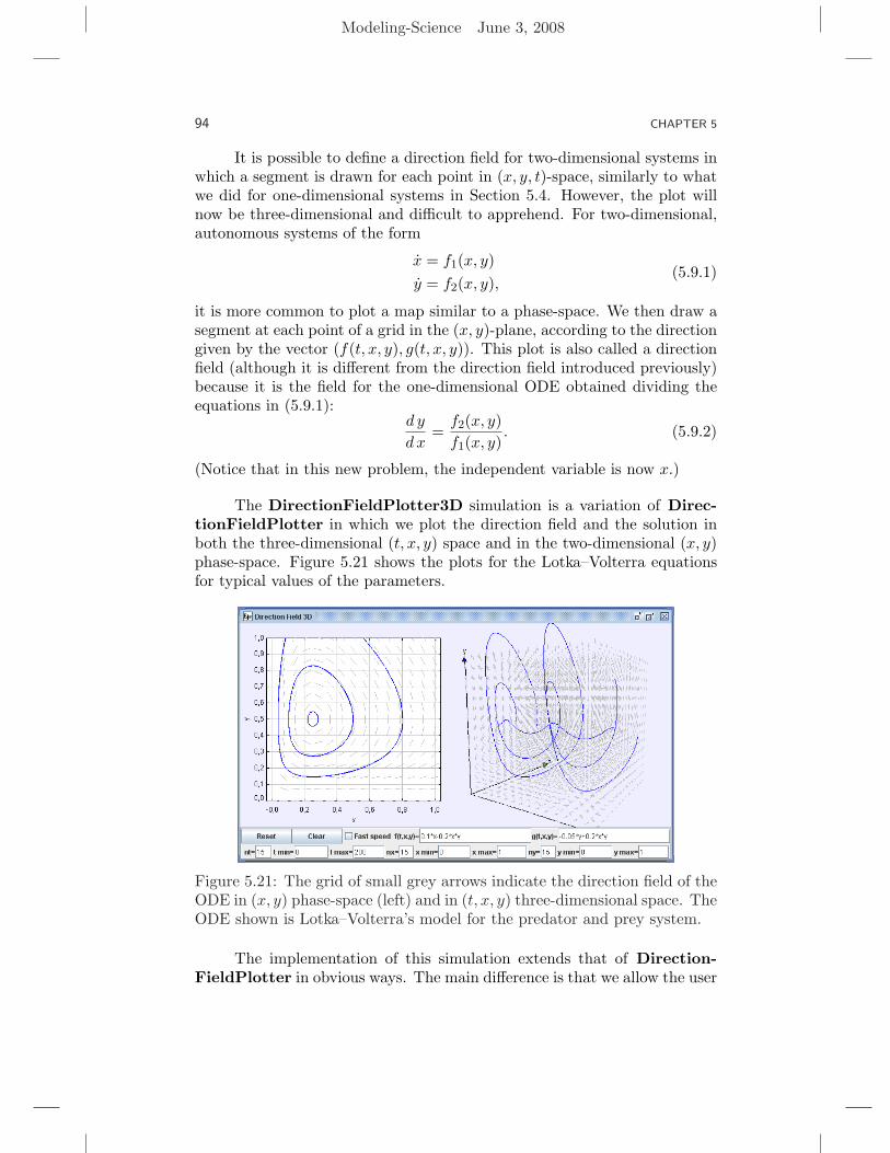
The DirectionFieldPlotter3D simulation is a variation of Direc-tionFieldPlotter in which we plot the direction field and the solution inboth the three-dimensional (t, x, y) space and in the two-dimensional (x, y)phase-space. Figure 5.21 shows the plots for the Lotka–Volterra equationsfor typical values of the parameters.
Figure 5.21: The grid of small grey arrows indicate the direction field of theODE in (x, y) phase-space (left) and in (t, x, y) three-dimensional space. TheODE shown is Lotka–Volterra’s model for the predator and prey system.
The implementation of this simulation extends that of Direction-FieldPlotter in obvious ways. The main difference is that we allow the user
Modeling-Science June 3, 2008
CONTINUOUS TIME MODELS 95
to select initial values for the populations, x0 and y0, which we take as ini-tial conditions at time t0 = 0. Hence, we always compute the solution curveforwards in time. The view of the simulation includes three-dimensionaldrawing elements and, although they behave in a similar way to two di-mensional elements in the plane, we must postpone their discussion untilChapter ??. But we thought it was important to be able to compare thethree- and two-dimensional views of the solution curve and the trajectory,respectively.
Notice that, in three-dimensional space, a solution curve never passestwice through the same point because t is always increasing. Uniquenessof solutions imply also that two solutions never cross. The behavior oftrajectories (x(t), y(t)) in phase-space can be different, since trajectories areprojections of the three-dimensional solution curves along the time axis.(To experience the feeling of this projection, left-click and drag the threedimensional scene to rotate it until the time axis points towards you.)
Exercise 5.22.Use the DirectionFieldPlotter3D simulation to plot the fields and trajec-tories of other two-dimensional systems. For instance, try a modification ofthe Lotka–Volterra model in which preys must compete among themselvesfor limited food supply:
x = a x− b xy − e x2,
y = −c y + d xy.(5.9.3)
Try e = 0.1 for the value of the parameters shown in Figure 5.21 and increasethe maximum allowed time to 500. The trajectories in phase-space loosetheir periodic behavior and spiral now towards an equilibrium point. Anequilibrium point existed also in the unmodified Lotka–Volterra model, butnow becomes attractive or asymptotically stable. This behavior means that,no matter their initial values, in the long run all populations approach aconstant value given by the coordinates of the equilibrium point. 2
Exercise 5.23.Does it make sense to plot the phase-space direction field for non-autonomoussystems? Judge by yourself. Enter the non-autonomous system
x = 0.05 (1.5 + sin(t/50))x− 0.2xy
y = 0.2xy − 0.05 y.(5.9.4)
in DirectionFieldPlotter3D and see how the field changes with time.Now trajectories in state-space can cross each other but also themselves ina non-periodic form. 2
Modeling-Science June 3, 2008
96 CHAPTER 5
PROBLEMS AND PROJECTS
Project 5.1 (Validation of Newton’s proportional cooling law). Before usingit extensively, models need to be validated by comparing their predictionsto known solutions of the problem or to experimental data. The Cooling-CoffeeData.txt file in this chapter’s data subdirectory contains data froma real experiment of a cooling cup of black and creamed coffee at a constantroom temperature. The fit of Figure 5.1 was created with the simulationCoolingCoffeeValidation, which reads the data and plots it, together withthe graph of the solution given by (5.1.2). Run this simulation, which hasinitially wrong parameters Tr and k, and try to adjust the parameters of thissolution so that both plots match to a reasonable degree of accuracy. [Hint:Run the simulation with the default parameters and right-click the experi-mental time series to bring in a data set tool as indicated in Appendix ??.Define a new fit according to equation (5.1.2). Use the parameters providedby the Autofit checkbox and re-run the model.]
The CoolingCoffeeValidation simulation uses the class ResourceLoader
from the package org.opensourcephysics.tools. This class handles accessto data typically found on disk files. The class takes care of finding the fileand converts the data in it into a ready-to-use format. See Table 5.1.
Table 5.1: Examples of methods in the class ResourceLoader.
getString(String path) Reads the contents of a text file andreturns it as a single String. Lines areseparated by the new line “\n” charac-ter.
getIcon(String path) Returns an object of thejavax.swing.ImageIcon class withthe contents of the graphic file.
getIcon(String path) Returns an object of thejava.applet.AudioClip class withthe contents of the audio file.
Project 5.2 (Validation of Newton’s proportional cooling law with changingoutside temperature). The CoolingCoffeeEditorValidation model usesthe ODE editor to solve equation (5.3.1) with an outside changing referencetemperature provided by data recorded experimentally. The file Cooling-WaterData.txt in the data directory provides records of the cooling ofhot water on an insulated steel cup and a regular cup, together with thesurrounding (cooler) temperature for 8 hours. 4 Reading the data file and
4The data was kindly recorded for us by Roger Frost (see http://www.rogerfrost.com) outdoorsin Cambridge, UK, on October 13th, 2007, starting at 9:00 AM.
Modeling-Science June 3, 2008
CONTINUOUS TIME MODELS 97
using it to create a usable Tr() method requires some Java technicalities.For instance, we use an object of the class java.util.ArrayList to accom-modate an unknown number of entry points. We also use a binary searchalgorithm to interpolate data in between the times provided by the file.
Use the simulation to try to adjust the parameter k so that the dataproduced by the theoretical model matches as closely as possible the exper-imental data. We found the data obtained from the isolated cup provided abetter fit than the regular cup, although fitting the first part of the graphis difficult in both cases. What is a possible explanation for this?
Project 5.3 (Harvesting in the Lotka–Volterra model). To provide a possibleexplanation of the decrease of percentage of the catch of food fish duringthe World War I period, Volterra modified the original model (5.5.3) tointroduce fishing. A model which uses constant-effort harvesting is given byequations
x = a x− b xy − h1 x,
y = −c y + d xy − h2 y.(5.9.5)
for non-negative constants h1 and h2. Modify the models of this chapterto show that a moderate amount of fishing increases the averages of preyand decreases that of predators. This was Volterra’s explanation of thephenomenon, since fishermen were involved in the war during the conflictand harvesting decreased noticeably during those years.
Project 5.4 (Dumped, driven pendulum). Although we will deal with pen-dula in detail in Chapter ??, modify the SimplePendulum model to inro-duce a dumping term and a driving force. The resulting equation is
θ = − g
Lsin(θ)− b ω + T (t). (5.9.6)
The positive parameter b provides a frictional force proportional to the an-gular velocity. The forcing term T (t) corresponds to an external torque onthe pendulum. Use a sinusoidal function of the form A sin(f t), where A isthe amplitude of the torque and f its frequency. Explore how the new termsaffect the phase-space portrait.
Project 5.5 (Length of a planet’s year). Run the SolarSystem simulationwith an increment of time of one day and compute approximately the lengthof the year for each of the planets. Notice the difference with the real lengths(224.70 days for Venus, 365.25 for the Earth, and 779.96 for Mars). Thereason is that we have used the average orbit velocity for each planet as thevelocity at its aphelion (the farthest point from the Sun). Explain why thisis incorrect and try to provide a more accurate value of the velocity at theaphelion (and hence of the year length) of the planets.
Modeling-Science June 3, 2008
98 CHAPTER 5
Project 5.6 (Logistic growth). (DRAFT TEXT) Use the techniques dis-cussed in this chapter to study the solution of the continuous LogisticGrowth model given by P = r(1 − P )P . Add harvesting (+Ho sin (2 pit)) and/ or migration to it +q(t) (Borelli and Coleman pg 127 and 125,resp.).
Project 5.7 (Trajectories in Dipole Fields). A charged particle in electric andmagnetic dipole fields.
Project 5.8 (Particles with Drag and Spin). Physics of sports.