58 Chapter III Finite element modelling and formulation development 3.1. General A structural analysis is performed on a model of the structure, not on the real structure, so the analysis can be no more accurate than the assumptions in the model. The model must represent the distribution and possible time variation of stiffness, strength, deformation capacity and mass of the structure with accuracy sufficient for the purpose of the analysis in the design process. In structural analysis, nonlinear modelling has evolved to address relevant issues including the variation in structural form, the influence of geometric nonlinearity and the nonlinear constitutive response of structural materials under serviceability and extreme loading conditions. In geotechnical analysis, on the other hand, developments have focused on, the constitutive modelling of different soils including pertinent nonlinear, coupling of mechanical/hydraulic/thermal/chemical processes in soils, and modelling of special boundary conditions, time dependent process such as consolidation and creep, and problem reduction. Though the structural field and geotechnical field have advanced computational tools offering sophisticated non-linear modelling in their respective fields, they fail together, to model an SSI problem to the same degree of sophistication. In this respect, existing advanced discipline-oriented computational tools are inadequate, on their own, for modelling a soil-structure interaction problem. One possibility is to augment existing software such that both soil and structure may be modelled to an equivalent level of sophistication though there remain significant technical challenges related to algorithmic and computational issues, particularly with reference to convergence. Another possibility is to develop new software integrating
Transcript
58
Chapter III
Finite element modelling and formulationdevelopment
3.1. General
A structural analysis is performed on a model of the structure, not on the real
structure, so the analysis can be no more accurate than the assumptions in the model.
The model must represent the distribution and possible time variation of stiffness,
strength, deformation capacity and mass of the structure with accuracy sufficient for the
purpose of the analysis in the design process.
In structural analysis, nonlinear modelling has evolved to address relevant issues
including the variation in structural form, the influence of geometric nonlinearity and the
nonlinear constitutive response of structural materials under serviceability and extreme
loading conditions.
In geotechnical analysis, on the other hand, developments have focused on, the
constitutive modelling of different soils including pertinent nonlinear, coupling of
mechanical/hydraulic/thermal/chemical processes in soils, and modelling of special
boundary conditions, time dependent process such as consolidation and creep, and
problem reduction.
Though the structural field and geotechnical field have advanced computational
tools offering sophisticated non-linear modelling in their respective fields, they fail
together, to model an SSI problem to the same degree of sophistication. In this respect,
existing advanced discipline-oriented computational tools are inadequate, on their own,
for modelling a soil-structure interaction problem.
One possibility is to augment existing software such that both soil and structure
may be modelled to an equivalent level of sophistication though there remain significant
technical challenges related to algorithmic and computational issues, particularly with
reference to convergence. Another possibility is to develop new software integrating
Non-linear Dynamic analysis of Soil Structure Interaction of Three Dimensional Structure For Varied Soil conditions
Chapter III
59
59
interdisciplinary computational model combining the features of both structural and
geotechnical aspects.
The powerful numerical tool like finite element method can be used to analyze the
problem considering the superstructure, foundation and the soil mass to act as single
integral compatible structural unit. As Finite element modelling and material modelling
depend on the method of dynamic analysis, summary of methods of analysis with their
advantages and disadvantages is presented below.
Further, of the four methods of SSI analyses viz., i) Elimination method, ii) Sub-structure
method, iii) Direct method and iv) Coupled methods of analysis, Direct Method of
analysis by using Finite element method is the only method that can be applied for non-
linear dynamic analysis of soil-structure-problem in time domain with the limitations of
other methods.
A suitable model can be picked up depending on the accuracy required and computational
facility available. Though it time consuming and necessitates development of a new soft
ware the present work deals with inclusion of non-linearity of soil in static and dynamic
SSI analysis of Space frame - foundation -soil system including the effects of infilled
masonry thoroughly investigating the effects of bonding between foundation and soil.
The solution of the problem of such interaction system needs a proper physical modelling
and numerical analysis to assess the more realistic and accurate structural behaviour of
the composite system.
3.2. Idealization of soil-structure interaction problem.
3.2.1. Modelling of superstructure
The various elements at macroscopic level in a three dimensional SSI problem are shown
in figure 3.1. The discretization of the domain of interaction system by adopting FEM
needs variety of isoparametric elements with different degrees of freedom.
All structures are three dimensional, but it is important to decide whether to use a
three-dimensional model or simpler two-dimensional models. The analysis methods are
the same whether the model is two dimensional or three dimensional. Generally, two
Non-linear Dynamic analysis of Soil Structure Interaction of Three Dimensional Structure For Varied Soil conditions
Chapter III
60
60
dimensional models are acceptable for buildings with regular configuration and minimal
torsion; otherwise, a three-dimensional model is necessary with a representation of the
floor diaphragms, foundation and soil. M. Leipold (2009) categorized various frame
elements in to four types as mentioned in figure 3.2.
In the most generalized form, superstructure of the building frames may be idealized as
three-dimensional space frame using two nodded beam elements. Plate element of
suitable dimension may be added to mimic the behaviour of slabs. The effects of infill
walls may be accounted for by imposing the loads of the walls on to the beams on which
they rest. This idealization appears (or assumed?) to be adequate for analyzing the
building frame under static gravity loading neglecting the contribution of infills to the
stiffness of structure.
When the infill panel is connected to the frame the total system acts as a
sing1e unit. These infill walls, though constructed as secondary structural elements,
behave as a constituent part of the structural system and determine the overall behaviour
of the structure, especially when it is subjected to seismic loads. However, designers tend
to treat these infill walls as “non-structural” and treat the frames as conventional frames, a
practice that is far from representing the true behaviour.
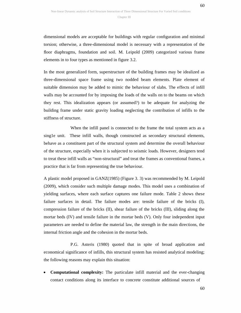
A plastic model proposed in GANZ(1985) (Figure 3. 3) was recommended by M. Leipold
(2009), which consider such multiple damage modes. This model uses a combination of
yielding surfaces, where each surface captures one failure mode. Table 2 shows these
failure surfaces in detail. The failure modes are: tensile failure of the bricks (I),
compression failure of the bricks (II), shear failure of the bricks (III), sliding along the
mortar beds (IV) and tensile failure in the mortar beds (V). Only four independent input
parameters are needed to define the material law, the strength in the main directions, the
internal friction angle and the cohesion in the mortar beds.
P.G. Asteris (1980) quoted that in spite of broad application and
economical significance of infills, this structural system has resisted analytical modeling;
the following reasons may explain this situation:
Computational complexity: The particulate infill material and the ever-changing
contact conditions along its interface to concrete constitute additional sources of
Non-linear Dynamic analysis of Soil Structure Interaction of Three Dimensional Structure For Varied Soil conditions
Chapter III
61
61
analytical burden. The real composite behavior of an infilled frame is a complex
statically indeterminate problem according to Smith (Smith 1966).
Structural uncertainities: The mechanical properties of masonry, as well as its
wedging conditions against the internal surface of the frame, depend strongly on local
construction conditions.
Non-linearity: The non-linear behavior of infilled frames depends on the separation
of masonry infill panel from the surrounding frame.
In the proposed approach, the infill is accounted for in the static as four nodded two
dimensional plane stress element. In dynamic analysis the infilled frame is idealized
either as a frame-diagonal strut system or as four nodded two dimensional plane stress
element depending on the diagonal distance after application of load increment.
When a lateral load is applied, the infill and the frame are getting separated over a large part of
the length of each side, and contact remains only adjacent to the corners at the ends of the
compression diagonal. The only accepted “natural” conditions between the infill and the frame are
either the contact or the separation condition. for which proposed finite element procedure is
implemented in following steps:
1. Initially each infill surrounded by frame elements on four sides is idealized as
plane stress element with four nodes and eight degrees of freedom.
2. After the first iteration Compute the nodal forces, displacements, and the stresses
at the corner points of the elements.
3. If the inclined distance between two opposite corners is less than the original
distance then the plane stress element is replaced by diagonal strut connecting the
corner. (Refer figure3. 3.)
3.2.2. Modelling of soil media
Soils are complex material consisting of a solid skeleton of grains in contact with each
other and voids filled with gas (air) and /or water or other fluid. The soil Skelton
transmits normal and shear forces at the grain contacts, and this Skelton of grains behaves
Non-linear Dynamic analysis of Soil Structure Interaction of Three Dimensional Structure For Varied Soil conditions
Chapter III
62
62
in a very complex manner that depends on a large number of factors, void ratio and
confining pressure being among the most important. However, the overall behavior of the
soil skeleton may be captured within principles of continuum mechanics (solid
mechanics). Interspersed in the void is water (incompressible fluid) and gas (compressible
fluid), each of which obeys its own physical laws. The mixture of grains, water, and air
produces a material that, in comparison with other engineering materials, is one of the
most difficult to characterize.
Since the philosophy of foundation design is to spread the load of the structure on to the
soil, ideal foundation modeling is that wherein the distribution of contact pressure is
simulated in a more realistic manner. The variation of pressure distribution depends on
the foundation behaviour (viz., rigid or flexible: two extreme situations) and nature of soil
deposit (clay or sand etc.). However, the mechanical behaviour of subsoil appears to be
utterly erratic and complex and it seems to be impossible to establish any mathematical
law that would conform to actual observation. In this context, simplicity of models, many
a time, becomes a prime consideration and they often yield reasonable results. Attempts
have been made by researchers to improve upon these models by some suitable
modifications to simulate the behaviour of soil more closely from physical standpoint.
With the development of numerical methods such as finite element and finite difference
methods it has become feasible to analyze and predict the behavior of complex soil
structure and soil/structure interaction problems. Such analyses depend considerably on
the representation of the relations between stresses and strains for the various materials
involved in the geotechnical structure. In numerical computation the relations between
stresses and strains in a given material are represented by constitutive model, consisting
of mathematical expressions that model the behavior of the soil in a single element,
determine the deformations and the possibility of failure of the structure. And it is
therefore important to characterize these materials accurately over the entire range of
stresses and strains to which they will become exposed. Thus, the purpose of a
constitutive model is to simulate the soil behavior with sufficient accuracy under all
loading conditions in the numerical computations.
Keeping the above points and the objectives of research in view and duly
considering the method of analysis, the soil is modeled with linear and non-linear
Non-linear Dynamic analysis of Soil Structure Interaction of Three Dimensional Structure For Varied Soil conditions
Chapter III
63
63
constitutive relations. In the present chapter finite element model is derived for linear
constitutive relations of soil. Non-linear model for soil and its development is discussed
in detail in chapter IV. In both cases soil is dicretized as brick element with eight nodes
having three degrees of freedom per node.
3.3. Finite element modelling
The solution of the problem of building frame-foundation beam-soil mass interaction
system needs a proper physical modeling and numerical analysis to access the more
realistic and accurate structural behaviour of the composite system. The powerful
numerical tool like finite element method can be used to analyze the problem considering
the superstructure, foundation and the soil mass to act as single integral compatible
structural unit. The material nonlinearity involved in the problem of soil structure-
interaction also needs a special numerical treatment. The discretization of the domain of
interaction system needs variety of isoparametric elements with different degrees of
freedom.
3.3.1 Types of elements
For the interaction of finite element static or dynamic analysis of a three dimensional
rigid jointed framed structure resting on soil, the following types of elements have been
adopted.
1) Columns and beams modelled as one dimensional element with six degrees of
freedom per node (three translational and three rotational dof).
2) In filled walls modelled as plane stress element with two translational degrees of
freedom per node.
3) Mat Foundation is modelled as plate element with five degrees of freedom per
node (three translational and two rotational degrees of freedoms).
4) Soil elements are modelled as eight noded brick element with three translational
degrees of freedom per node.
3.3.2 Stiffness matrix of beam element:-
A typical beam/ column element of the structure is shown in figure 3.5. In local co-
Non-linear Dynamic analysis of Soil Structure Interaction of Three Dimensional Structure For Varied Soil conditions
Chapter III
64
64
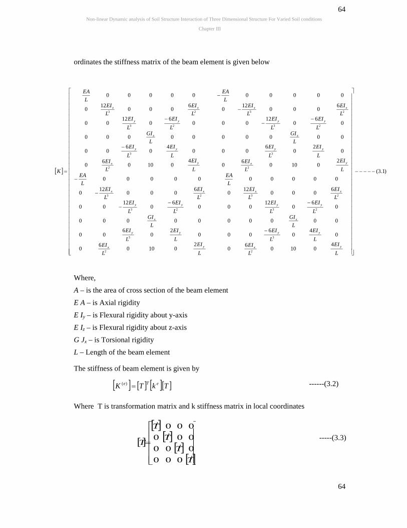
ordinates the stiffness matrix of the beam element is given below
Where,
A – is the area of cross section of the beam element
E A – is Axial rigidity
E Iy – is Flexural rigidity about y-axis
E Iz – is Flexural rigidity about z-axis
G Jx – is Torsional rigidity
L – Length of the beam element
The stiffness of beam element is given by
Where T is transformation matrix and k stiffness matrix in local coordinates
)1.3(
40100
60
04
06
00
00000
06
012
00
6000
120
00000
20100
60
02
06
00
00000
06
012
00
6000
120
00000
20100
60
02
06
00
00000
06
012
00
6000
120
00000
40100
60
04
06
00
00000
06
012
00
6000
120
00000
2
3
23
23
2
3
23
23
2
3
23
23
2
3
23
23
L
EI
L
EIL
EI
L
EIL
GIL
EI
L
EIL
EI
L
EIL
EA
L
EI
L
EIL
EI
L
EIL
GIL
EI
L
EIL
EI
L
EIL
EAL
EI
L
EIL
EI
L
EIL
GIL
EI
L
EIL
EI
L
EIL
EA
L
EI
L
EIL
EI
L
EIL
GIL
EI
L
EIL
EI
L
EIL
EA
K
yx
yy
x
yy
xx
yx
yy
x
yy
xx
yx
yy
x
yy
xx
yx
yy
x
yy
xx
l
l
l
l
T
T
T
T
T
000
000
000
000
-----(3.3)
TkTK eTe)( ------(3.2)
Non-linear Dynamic analysis of Soil Structure Interaction of Three Dimensional Structure For Varied Soil conditions
Chapter III
65
65
)4.3(cos
22
22
22
22
22
22
yx
xyxzy
zx
xyx
zx
xyxzx
zx
xyx
zyx
l
CC
CosCSinCCSinCC
CC
CosCSinCC
CC
SinCCosCCCosCC
CC
SinCCCCCC
T
Where Cx , Cy and Cz are direction cosines of the beam with respect to global axes. is
the angle of twist of plane of symmetry of cross section with respect to x-y plane. The
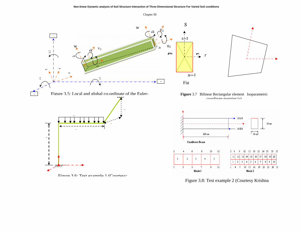
element has been implemented in the three-dimensional finite element software and
checked against simple example 1., given in Rajashekharan et al (2000). Shown in figure
3.6.
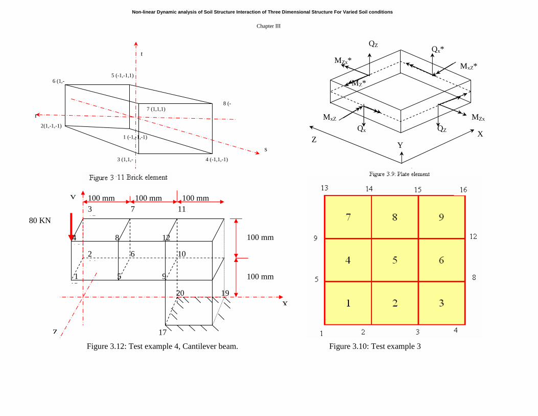
3.3.3 Stiffness of Plane stress element
With the shape functions in terms of (r, s) co-ordinate system, the coordinates of any
point can be expressed in terms of (x, y) co-ordinates as
Where N =
In this case since the number of nodes are 4, n=4
dvBCk
bygiveniselementanof[k]t
B
matrixStiffness
-------
(3.7)
Where
[B], is strain displacement matrix
i
n
nii usrNsru ),(),(
i
n
nii vsrNsrv ),(),(
i
n
nii xsrNsrx ),(),(
i
n
nii ysrNsry ),(),(
-----(3.5)
------(3.6)4
)1)(1( ssrr ii
Non-linear Dynamic analysis of Soil Structure Interaction of Three Dimensional Structure For Varied Soil conditions
Chapter III
66
66
[C], is constitutive matrix
------(3.8)
Where, t is the thickness of 2-d element.
If the coordinates are transferred to natural coordinates ),( sr we have
-------(3.9)
Where |J| is determinant of Jacobian matrix [J]
The constitutive matrix for a plane stress condition is given by following equation
100
01
01
1 2
EC -----(3.10)
The Jacobian matrix
The Jacobian matrix in terms of shape functions and nodal coordinates is given by
dsdJBtt
rBCk
dsdrJdydx
dydxBCk
dydx tBCk
t
t
Bt
B
[J]
][
*22
*21
*12
*111-
s
rJJ
JJ
s
r
y
x
y
xJ
s
r
y
x
s
y
s
xr
y
r
x
s
r
------(3.11)
----(3.12)
----(3.13)
Non-linear Dynamic analysis of Soil Structure Interaction of Three Dimensional Structure For Varied Soil conditions
Chapter III
67
67
n
i i
n
i i
n
i i
n
i i
ys
xs
yr
xr
1
i
1
i
1
i
1
i
*N
*N
*N
*N
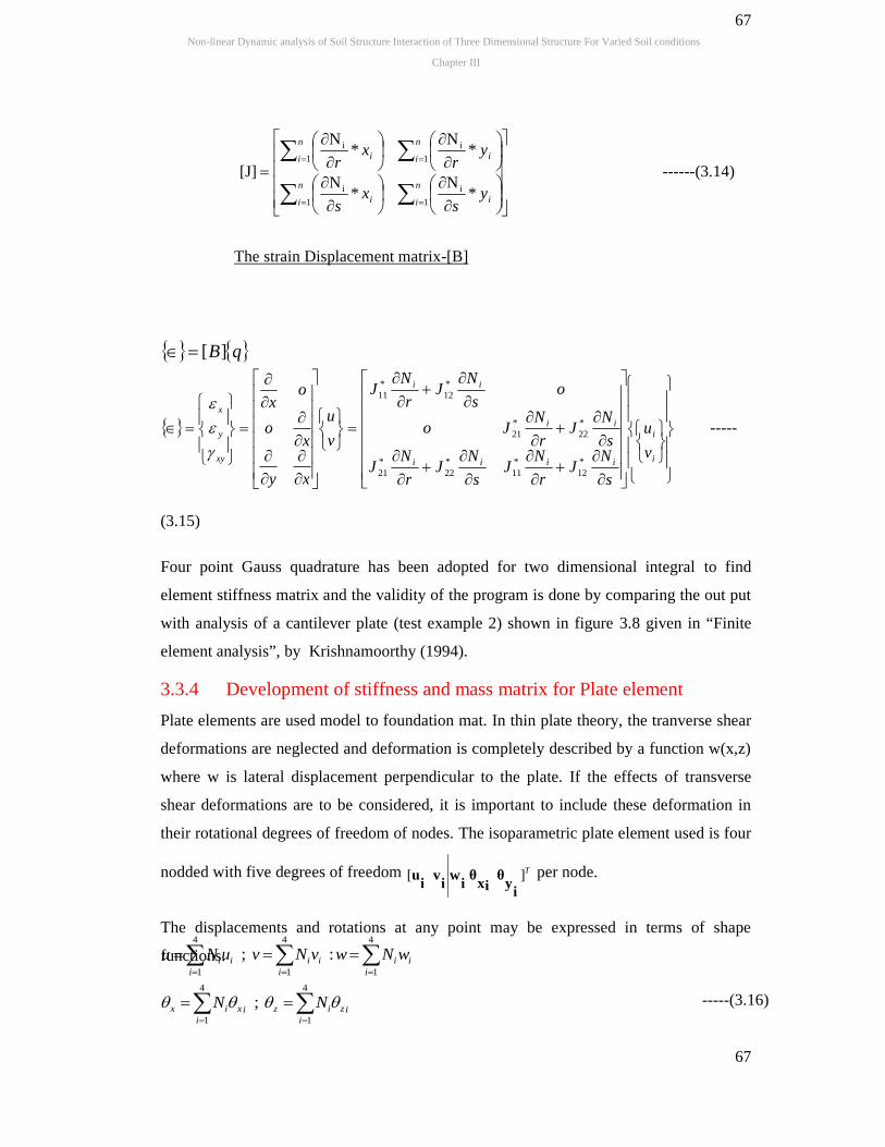
[J] ------(3.14)
The strain Displacement matrix-[B]
qB][
i
i
iiii
ii
ii
xy
y
x
v
u
s
NJ
r
NJ
s
NJ
r
NJ
s
NJ
r
NJo
os
NJ
r
NJ
v
u
xy
xo
ox
*12
*11
*22
*21
*22
*21
*12
*11
-----
(3.15)
Four point Gauss quadrature has been adopted for two dimensional integral to find
element stiffness matrix and the validity of the program is done by comparing the out put
with analysis of a cantilever plate (test example 2) shown in figure 3.8 given in “Finite
element analysis”, by Krishnamoorthy (1994).
3.3.4 Development of stiffness and mass matrix for Plate element
Plate elements are used model to foundation mat. In thin plate theory, the tranverse shear
deformations are neglected and deformation is completely described by a function w(x,z)
where w is lateral displacement perpendicular to the plate. If the effects of transverse
shear deformations are to be considered, it is important to include these deformation in
their rotational degrees of freedom of nodes. The isoparametric plate element used is four
nodded with five degrees of freedom T][iyθ
ixθiwiviu per node.
The displacements and rotations at any point may be expressed in terms of shape
functions.
;
:;
4
1
4
1
4
1
4
1
4
1
iiziz
iixix
iii
iii
iii
NN
wNwvNvuNu
-----(3.16)
Non-linear Dynamic analysis of Soil Structure Interaction of Three Dimensional Structure For Varied Soil conditions
Chapter III
68
68
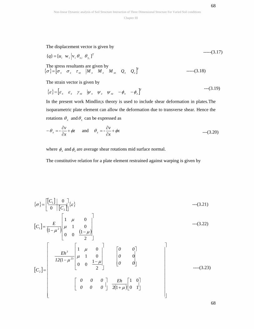
The displacement vector is given by
Tiiuq ]v w[}{
iyxii
The stress resultants are given by
The strain vector is given by
Tzxxzzxxzzx
In the present work Mindlin;s theory is used to include shear deformation in plates.The
isoparametric plate element can allow the deformation due to transverse shear. Hence the
rotations zand x can be expressed as
where zand x are average shear rotations mid surface normal.
The constitutive relation for a plate element restrained against warping is given by
-----(3.17)
---(3.19)
-and- xx
vz
x
vzx
---(3.20)
-----(3.18) Tzxxzzxxzzx QQMMM
10
01
12
0
2
100
01
01
1(
2
100
01
01
1
0
0
)2
2
21
2
1
Eh
000
000
00
0
00
12
Eh
C
EC
C
C
3
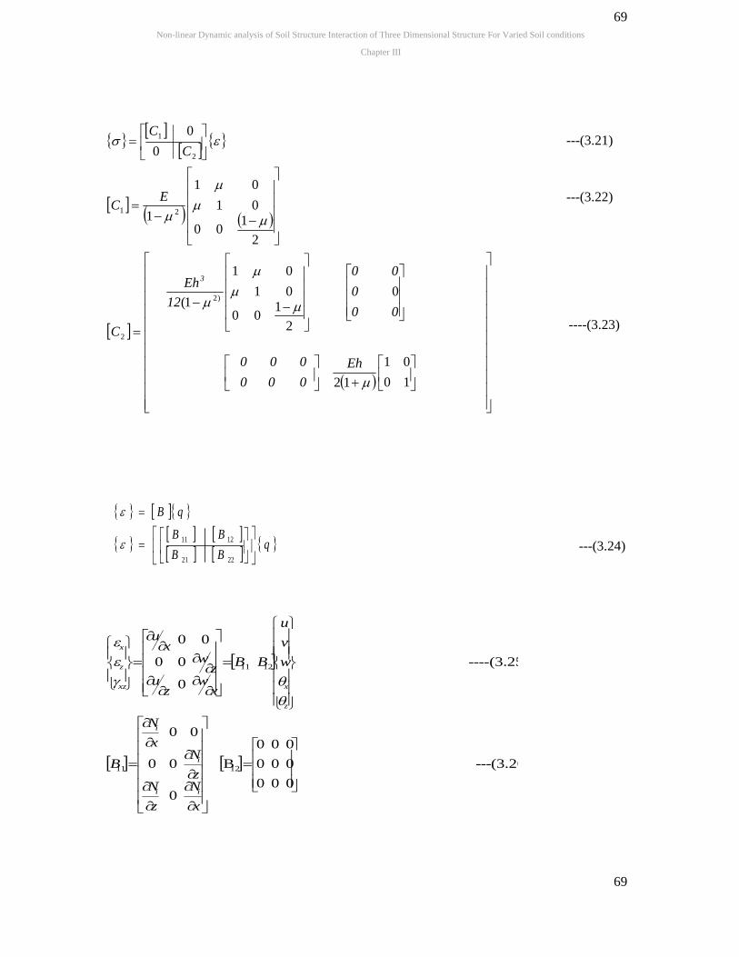
---(3.21)
---(3.22)
----(3.23)
Non-linear Dynamic analysis of Soil Structure Interaction of Three Dimensional Structure For Varied Soil conditions
Chapter III
69
69
10
01
12
0
2
100
01
01
1(
2
100
01
01
1
0
0
)2
2
21
2
1
Eh
000
000
00
0
00
12
Eh
C
EC
C
C
3
---(3.21)
---(3.22)
----(3.23)
2221
1211 qBB
BB
qB
---(3.24)
(3.26)---
000
000
000
B
0
00
00
-(3.25)---
0
00
00
1211
1211
x
N
z
Nz
Nx
N
B
w
v
u
BB
xw
zu
zw
xu
ii
i
i
z
xxz
z
x
Non-linear Dynamic analysis of Soil Structure Interaction of Three Dimensional Structure For Varied Soil conditions
Chapter III
70
70
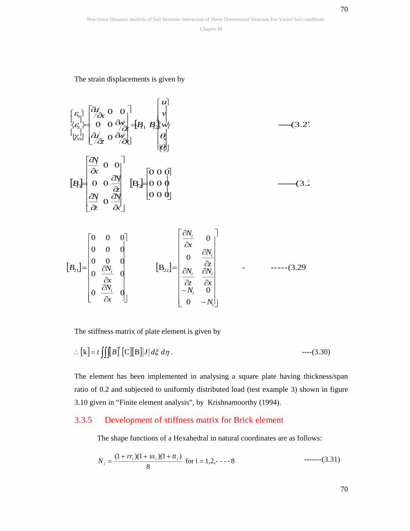
(3.28)-------
000
000
000
B
0
00
00
(3.27)-----
0
00
00
1211
1211
x
N
z
Nz
Nx
N
B
w
v
u
BB
xw
zu
zw
xu
ii
i
i
z
xxz
z
x
The strain displacements is given by
The stiffness matrix of plate element is given by
ddJBtt
BCk . ----(3.30)
The element has been implemented in analysing a square plate having thickness/span
ratio of 0.2 and subjected to uniformly distributed load (test example 3) shown in figure
3.10 given in “Finite element analysis”, by Krishnamoorthy (1994).
3.3.5 Development of stiffness matrix for Brick element
The shape functions of a Hexahedral in natural coordinates are as follows:
-------(3.31)8---1,2,-ifor8
)1)(1)(1(
iii
i
ttssrrN
(3.29)------
0
0
0
0
B
00
00
000
000
000
2221
i
i
ii
i
i
i
i
N
Nx
N
z
Nz
Nx
N
x
Nx
NB
Non-linear Dynamic analysis of Soil Structure Interaction of Three Dimensional Structure For Varied Soil conditions
Chapter III
71
71
Where r, s, t are natural coordinates and ri,, si and ti are values of natural
coordinates for i. Refer figure 3.11
freedomofdegreesnodal theiswhere
8
1
1
1
8
1i
8
1i
8
1i
QB
zuxwywzv
xvyuzwyvxu
wvuQ
QN
w
wv
u
N
wN
vN
uN
w
v
u
xz
yz
xy
z
y
x
Tiii
ii
ii
ii
821Bismatrixntdisplacemestrain thewhere BBB
The derivatives of [B] is obtained by chain rule
x
N
z
Ny
N
z
Nx
N
y
Nz
Ny
Nx
N
B
ii
ii
ii
i
i
i
i
0
0
0
00
00
00
---(3.32)
---(3.33)
---(3.34)
---(3.35)
--(3.36)
Consider
zN
yN
xN
J
zN
yN
xN
tztytx
szsysx
rzryrx
tN
sN
rN
i
i
i
i
i
i
i
i
i
Non-linear Dynamic analysis of Soil Structure Interaction of Three Dimensional Structure For Varied Soil conditions
Chapter III
72
72
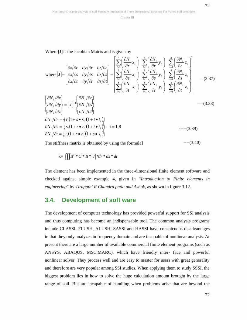
The stiffness matrix is obtained by using the formula]
k= dtdsdrJBCB t ******
The element has been implemented in the three-dimensional finite element software and
checked against simple example 4, given in “Introduction to Finite elements in
engineering” by Tirupathi R Chandra patla and Ashok, as shown in figure 3.12.
3.4. Development of soft ware
The development of computer technology has provided powerful support for SSI analysis
and thus computing has become an indispensable tool. The common analysis programs
include CLASSI, FLUSH, ALUSH, SASSI and HASSI have conspicuous disadvantages
in that they only analyzes in frequency domain and are incapable of nonlinear analysis. At
present there are a large number of available commercial finite element programs (such as
ANSYS, ABAQUS, MSC.MARC), which have friendly inter- face and powerful
nonlinear solver. They process well and are easy to master for users with great generality
and therefore are very popular among SSI studies. When applying them to study SSSI, the
biggest problem lies in how to solve the huge calculation amount brought by the large
range of soil. But are incapable of handling when problems arise that are beyond the
----(3.40)
1,8i
11
11
11
Jwhere
bygivenisandMatrixJacobian theis[J]Where
81
81
81
1
8
1
8
1
8
1
8
1
8
1
8
1
8
1
8
1
8
1
iiii
iiii
iiii
i
i
i
i
i
i
ii
i
ii
i
ii
i
ii
i
ii
i
ii
i
ii
i
ii
i
ii
i
ssrrttN
ttrrssN
ttssrrN
tN
sN
rN
J
zN
yN
xN
zt
Ny
t
Nx
t
N
zs
Ny
s
Nx
s
N
zr
Ny
r
Nx
r
N
tztytx
szsysx
rzryrx
-----(3.39)
----(3.38)
--(3.37)
Non-linear Dynamic analysis of Soil Structure Interaction of Three Dimensional Structure For Varied Soil conditions
Chapter III
73
73
standard capability of the tool.
Since many individuals write programs for a broad range of applications, most high-level
computer languages, like FORTRAN and C, have rich capabilities. Although some
engineers might need to tap the full range of these capabilities, most merely require the
ability to perform engineering-oriented numerical calculations.
Finite element analysis is a method for numerical solution of field problems and a field
problem is the spatial distribution of one or more dependent variables. The region of
interest for the distribution of this field is mapped or geometrically defined by nodes and
than discretized into and represented by “finite” geometric units in which the field
variable is allowed to vary from node to node in a way described by a polynomial
function. The location of the nodes is the locations where the value of field of interest is
sought. The units, which are defined by “nodes”, are called the “elements”, and the
particular assembly of these elements is called the mesh. The algebraic equations within
these elements are solved for the unknown field quantities at the nodes.
The solution procedure for a time-independent FEA can be summarized as:
1. Description the element behavior through matrices.
2. Assembly of the individual matrices through element connection.
3. Establishing the loading and boundary conditions.
4. Determination of nodal quantities through algebraic equations created by a system of
structure matrix, loading and the boundary conditions.
5. Computation of gradients.
In the present research FORTRAN 77 is used to take following input for a Static SSI
analysis:
Young’s modulus and rigidity modulus, and unit weight of beam material,
Young’s modulus of soil at top and bottom, unit weight and poisons ratio of soil.
Young’s modulus, rigidity modulus, unit weight and poisons ratio of foundation
material.
Young’s modulus, unit weight and poisons ratio of infills material.
Non-linear Dynamic analysis of Soil Structure Interaction of Three Dimensional Structure For Varied Soil conditions
Chapter III
74
74
Breadth, depth and load on beams in X-direction.
Breadth, depth and load on beams in Z-direction.
Breadth and depth of column.
Length, breadth and depth of mat/ isolated footings and Load on mat foundation.
Number of layers of soil in X, Y and Z directions.
Thickness of soil layers in X, Y and Z directions.
Number of plate elements (representing raft foundation or isolated footing) and
soil elements beyond column edge in X and Z directions towards boundary.
Number of plate elements (isolated footing) on either side of columns in X and Z
directions.
Number of columns in X and Z directions
Number of soil elements between columns in X and Z direction.
The matrix displacement equations are linear simultaneous equations. The features of
matrix displacement equations are as follows
i) The matrix is having diagonal dominance and is positive definite. Hence in
the solution process there is no need to rearrange the equations to get
diagonal dominance.
ii) The matrix is symmetric.
iii) The matrix is having banded nature i.e., the nonzero elements of stiffness
matrix are concentrated near the diagonal of the stiffness matrix.
Considerable saving can be achieved in memory of computers by avoiding
storage of zero values of stiffness matrix.
Since the size of stiffness matrix is very large it results in shortage of memory. Hence
optimizing memory requirement to store stiffness matrix values becomes essential. The
line separating the top zero elements from the first non – zero element is called the
Skyline. In this system of storage, if there are zero elements at the top of a column, only
the elements from the first non-zero value need to be stored. This method is called
Non-linear Dynamic analysis of Soil Structure Interaction of Three Dimensional Structure For Varied Soil conditions
Chapter III
75
75
Skyline storage and is used in the present work.
Contents of the global stiffness matrix before reduction is often has less than 5%
number of non-zero elements and perhaps less than 1% non-zero elements if there are
thousands of degrees of freedom. During reduction of stiffness a direct solver changes
most zeros between the skyline and diagonal to nonzero, but leaves zeroes above the
skyline intact, so the matrix remains sparse. A profile or skyline single array storage
scheme is adopted to save the memory space needed in the storage of the matrices. An
active column profile (skyline) solution algorithm is employed in the equation solution
module to solve the equations efficiently. The use of this method with an active column
profile storage scheme leads to a very compact program where it is very easy to use
vector dot product routines to effect the triangular decomposition and forward reduction.
This computational advantage is very important to modern computers which are vector
oriented. Therefore software exploit this sparcity by using compact storage formats, so
that nonzero elements are neither stored nor processed. Three subroutines COLUMNH,
CADNUM and PASSEM were developed for static analysis. The subroutines which are
developed in dynamic analysis are dealt in chapter---.
To accomplish the above steps, in the present research, FORTRAN 77 is used and
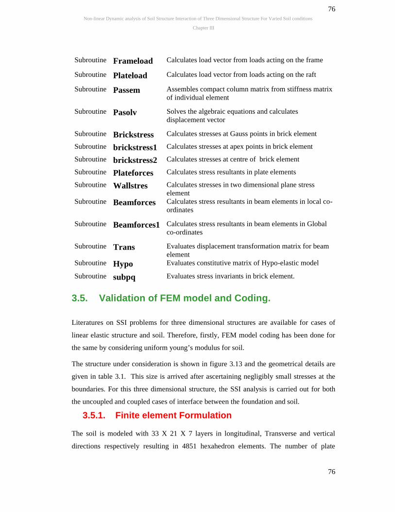
following subroutines are developed:
Subroutine Mesh Generates Finite element mesh, generates element noderelationship, coordinates of nodes, relationship betweenelement and Global degrees of freedom .
Subroutine Columh Calculates column height and size of compact columnmatrix.
Subroutine cadnum Gives the diagonal address of diagonal elements incompact column matrix.