Chapter 5: Terrain Rendering in Frostbite Using Procedural Shader Splatting 38 Chapter 5 Terrain Rendering in Frostbite Using Procedural Shader Splatting Johan Andersson 7 5.1 Introduction Many modern games take place in outdoor environments. While there has been much research into geometrical LOD solutions, the texturing and shading solutions used in real-time applications is usually quite basic and non-flexible, which often result in lack of detail either up close, in a distance, or at high angles. One of the more common approaches for terrain texturing is to combine low-resolution unique color maps (Figure 1) for low-frequency details with multiple tiled detail maps for high-frequency details that are blended in at certain distance to the camera. This gives artists good control over the lower frequencies as they can paint or generate the color maps however they want. For the detail mapping there are multiple methods that can be used. In Battlefield 2, a 256 m 2 patch of the terrain could have up to six different tiling detail maps that were blended together using one or two three-component unique detail mask textures (Figure 4) that controlled the visibility of the individual detail maps. Artists would paint or generate the detail masks just as for the color map. 7 email: [email protected]Figure 1. Terrain color map from Battlefield 2
Transcript
Chapter 5: Terrain Rendering in Frostbite Using Procedural Shader Splatting
38
Chapter 5
Terrain Rendering in Frostbite Using Procedural Shader
Splatting
Johan Andersson 7
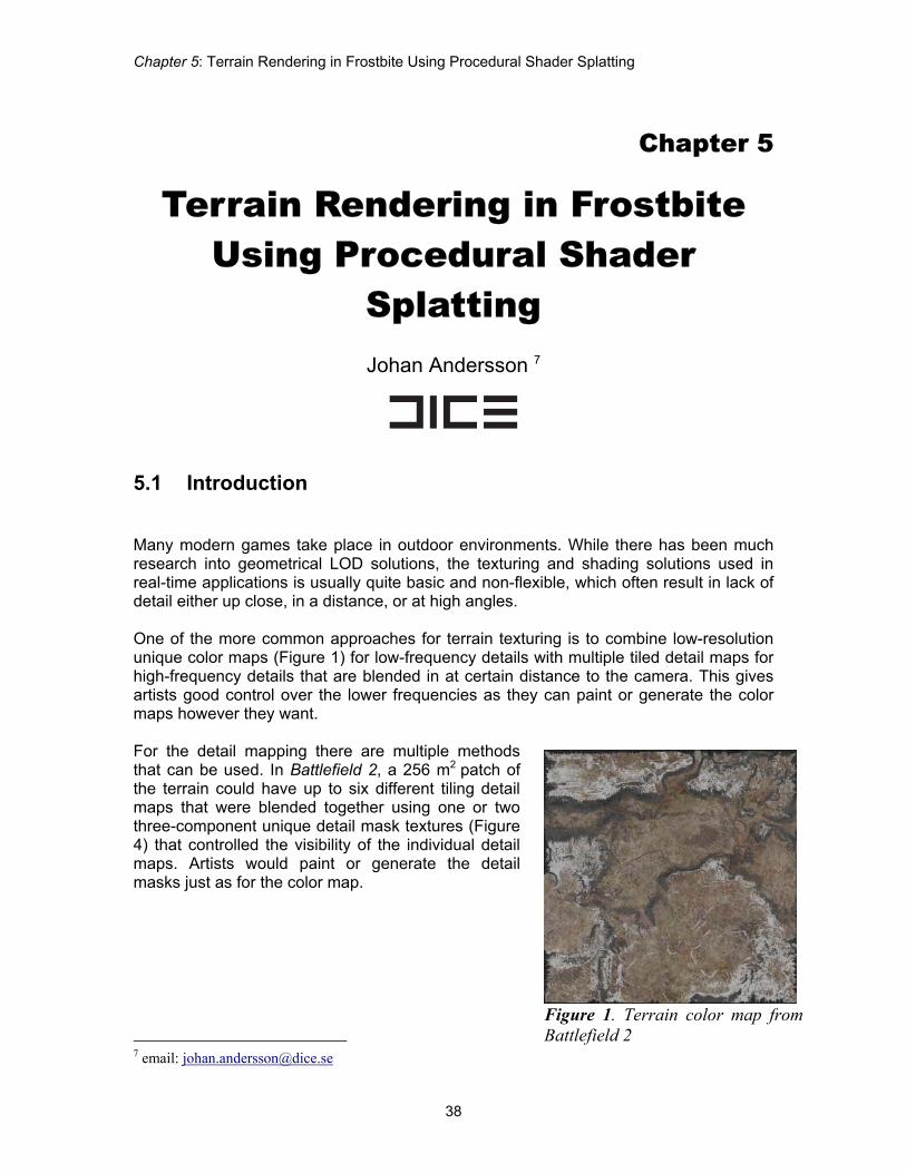
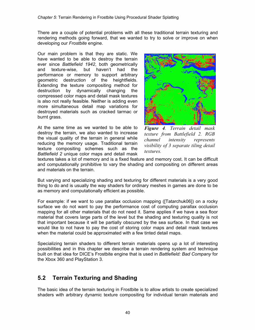
5.1 Introduction Many modern games take place in outdoor environments. While there has been much research into geometrical LOD solutions, the texturing and shading solutions used in real-time applications is usually quite basic and non-flexible, which often result in lack of detail either up close, in a distance, or at high angles. One of the more common approaches for terrain texturing is to combine low-resolution unique color maps (Figure 1) for low-frequency details with multiple tiled detail maps for high-frequency details that are blended in at certain distance to the camera. This gives artists good control over the lower frequencies as they can paint or generate the color maps however they want. For the detail mapping there are multiple methods that can be used. In Battlefield 2, a 256 m2 patch of the terrain could have up to six different tiling detail maps that were blended together using one or two three-component unique detail mask textures (Figure 4) that controlled the visibility of the individual detail maps. Artists would paint or generate the detail masks just as for the color map.
Advanced Real-Time Rendering in 3D Graphics and Games Course – SIGGRAPH 2007
39
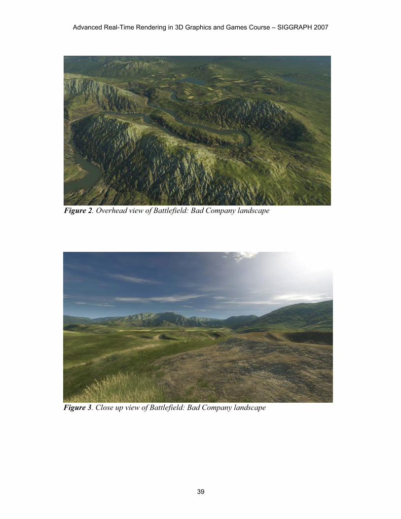
Figure 3. Close up view of Battlefield: Bad Company landscape
Figure 2. Overhead view of Battlefield: Bad Company landscape
Chapter 5: Terrain Rendering in Frostbite Using Procedural Shader Splatting
40
There are a couple of potential problems with all these traditional terrain texturing and rendering methods going forward, that we wanted to try to solve or improve on when developing our Frostbite engine. Our main problem is that they are static. We have wanted to be able to destroy the terrain ever since Battlefield 1942, both geometrically and texture-wise, but haven’t had the performance or memory to support arbitrary geometric destruction of the heightfields. Extending the texture compositing method for destruction by dynamically changing the compressed color maps and detail mask textures is also not really feasible. Neither is adding even more simultaneous detail map variations for destroyed materials such as cracked tarmac or burnt grass. At the same time as we wanted to be able to destroy the terrain, we also wanted to increase the visual quality of the terrain in general while reducing the memory usage. Traditional terrain texture compositing schemes such as the Battlefield 2 unique color maps and detail mask textures takes a lot of memory and is a fixed feature and memory cost. It can be difficult and computationally prohibitive to vary the shading and compositing on different areas and materials on the terrain. But varying and specializing shading and texturing for different materials is a very good thing to do and is usually the way shaders for ordinary meshes in games are done to be as memory and computationally efficient as possible. For example: if we want to use parallax occlusion mapping ([Tatarchuk06]) on a rocky surface we do not want to pay the performance cost of computing parallax occlusion mapping for all other materials that do not need it. Same applies if we have a sea floor material that covers large parts of the level but the shading and texturing quality is not that important because it will be partially obscured by the sea surface. In that case we would like to not have to pay the cost of storing color maps and detail mask textures when the material could be approximated with a few tinted detail maps. Specializing terrain shaders to different terrain materials opens up a lot of interesting possibilities and in this chapter we describe a terrain rendering system and technique built on that idea for DICE’s Frostbite engine that is used in Battlefield: Bad Company for the Xbox 360 and PlayStation 3. 5.2 Terrain Texturing and Shading The basic idea of the terrain texturing in Frostbite is to allow artists to create specialized shaders with arbitrary dynamic texture compositing for individual terrain materials and
Figure 4. Terrain detail mask texture from Battlefield 2. RGB channel intensity represents visibility of 3 separate tiling detail textures.
Advanced Real-Time Rendering in 3D Graphics and Games Course – SIGGRAPH 2007
41
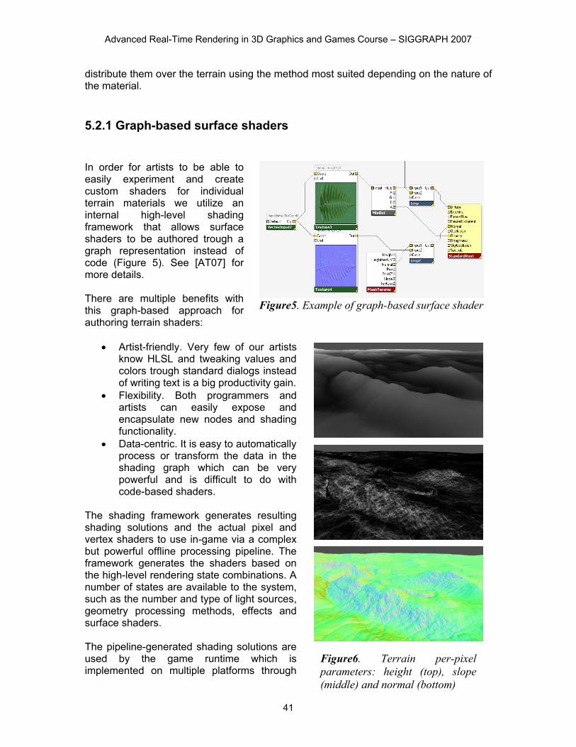
Figure6. Terrain per-pixel parameters: height (top), slope (middle) and normal (bottom)
distribute them over the terrain using the method most suited depending on the nature of the material.
5.2.1 Graph-based surface shaders In order for artists to be able to easily experiment and create custom shaders for individual terrain materials we utilize an internal high-level shading framework that allows surface shaders to be authored trough a graph representation instead of code (Figure 5). See [AT07] for more details. There are multiple benefits with this graph-based approach for authoring terrain shaders:
x Artist-friendly. Very few of our artists know HLSL and tweaking values and colors trough standard dialogs instead of writing text is a big productivity gain.
x Flexibility. Both programmers and artists can easily expose and encapsulate new nodes and shading functionality.
x Data-centric. It is easy to automatically process or transform the data in the shading graph which can be very powerful and is difficult to do with code-based shaders.
The shading framework generates resulting shading solutions and the actual pixel and vertex shaders to use in-game via a complex but powerful offline processing pipeline. The framework generates the shaders based on the high-level rendering state combinations. A number of states are available to the system, such as the number and type of light sources, geometry processing methods, effects and surface shaders. The pipeline-generated shading solutions are used by the game runtime which is implemented on multiple platforms through
Figure5. Example of graph-based surface shader
Chapter 5: Terrain Rendering in Frostbite Using Procedural Shader Splatting
42
rendering backends for DirectX9, Xbox 360, PlayStation 3 and Direct3D10. It handles dispatching commands to the GPU and can be quite thin by following the shading solutions that contain instructions on exactly how to setup the rendering. Along with enabling graph-based shader development, we realized the need to support flexible and powerful code-based shader block development in our framework. Often, both artists and programmers may want to take advantage of custom complex functions and reuse them throughout the shader network. As a solution to this problem, we introduce instance shaders - shader graphs with explicit inputs and outputs that can be instanced and reused inside other shaders. Through this concept, we can hierarchically encapsulate parts of shaders and create very complex shader graph networks while still being manageable and efficient. This functionality allows the shader networks to be easily extensible. Much of the terrain shading and texturing functionality is implemented with instance shaders. General data transformation and optimization capabilities in the pipeline that operate (mostly) on the graph-level are utilized to combine multiple techniques to create long single-pass shaders.
5.2.2 Procedural parameters Over the last decade, the computational power of consumer GPUs has been exceeding the Moore’s law, graphics chips becoming faster and faster with every generation. At the same time, memory size and bandwidth increases do not match the jumps in GPU compute. Realizing this trend, it makes sense to try to calculate much of the terrain shading and texture compositing in the shaders instead of storing it all in textures. There are many interesting procedural techniques for terrain texturing and generation, but most would require multi-pass rendering into cached textures for real-time usage or can be expensive and difficult to mipmap correctly (such as GPU Wang Tiles in [Wei 03]). We have chosen to start with a very simple concept of calculating and exposing three procedural parameters to the graph-based terrain shaders (Figure 6) for performance reasons:
x Height (meters) x Slope (0.0 = 0 degrees, 1.0 = 90°) x Normal (world-space)
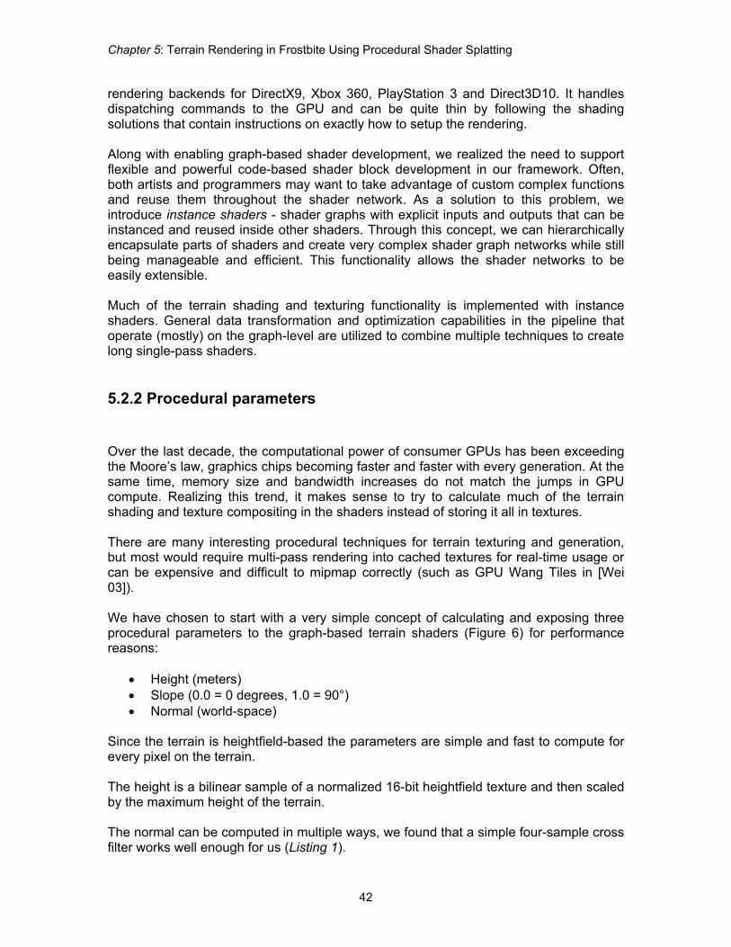
Since the terrain is heightfield-based the parameters are simple and fast to compute for every pixel on the terrain. The height is a bilinear sample of a normalized 16-bit heightfield texture and then scaled by the maximum height of the terrain. The normal can be computed in multiple ways, we found that a simple four-sample cross filter works well enough for us (Listing 1).
Advanced Real-Time Rendering in 3D Graphics and Games Course – SIGGRAPH 2007
43
The slope is one minus the y-component of the normal.
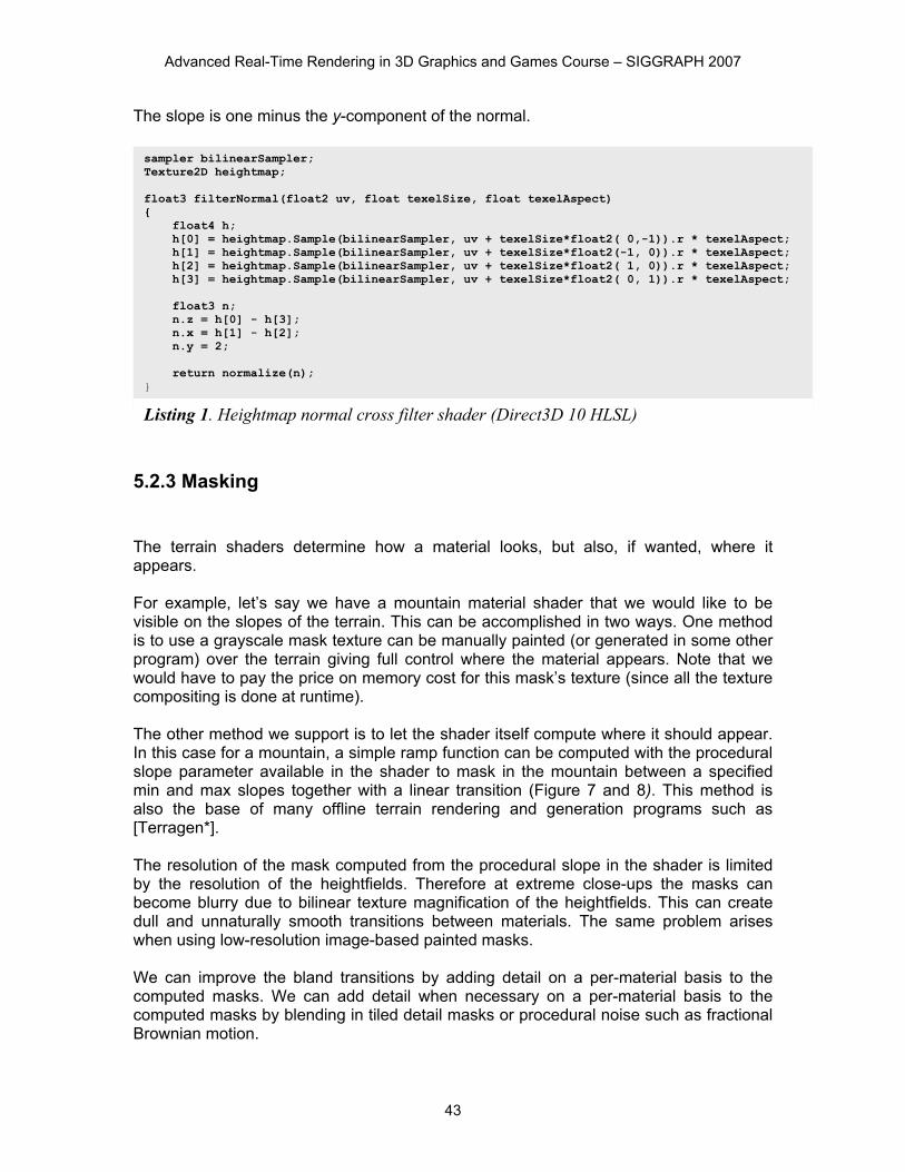
5.2.3 Masking The terrain shaders determine how a material looks, but also, if wanted, where it appears. For example, let’s say we have a mountain material shader that we would like to be visible on the slopes of the terrain. This can be accomplished in two ways. One method is to use a grayscale mask texture can be manually painted (or generated in some other program) over the terrain giving full control where the material appears. Note that we would have to pay the price on memory cost for this mask’s texture (since all the texture compositing is done at runtime). The other method we support is to let the shader itself compute where it should appear. In this case for a mountain, a simple ramp function can be computed with the procedural slope parameter available in the shader to mask in the mountain between a specified min and max slopes together with a linear transition (Figure 7 and 8). This method is also the base of many offline terrain rendering and generation programs such as [Terragen*]. The resolution of the mask computed from the procedural slope in the shader is limited by the resolution of the heightfields. Therefore at extreme close-ups the masks can become blurry due to bilinear texture magnification of the heightfields. This can create dull and unnaturally smooth transitions between materials. The same problem arises when using low-resolution image-based painted masks. We can improve the bland transitions by adding detail on a per-material basis to the computed masks. We can add detail when necessary on a per-material basis to the computed masks by blending in tiled detail masks or procedural noise such as fractional Brownian motion.
Listing 1. Heightmap normal cross filter shader (Direct3D 10 HLSL)
Chapter 5: Terrain Rendering in Frostbite Using Procedural Shader Splatting
44
Computing noise in pixel shaders can yield high quality and can be reasonably fast on modern GPUs ([Tatarchuk 07]) but for our purpose where we would like to compute multiple octaves for multiple materials it is still computationally prohibitive.
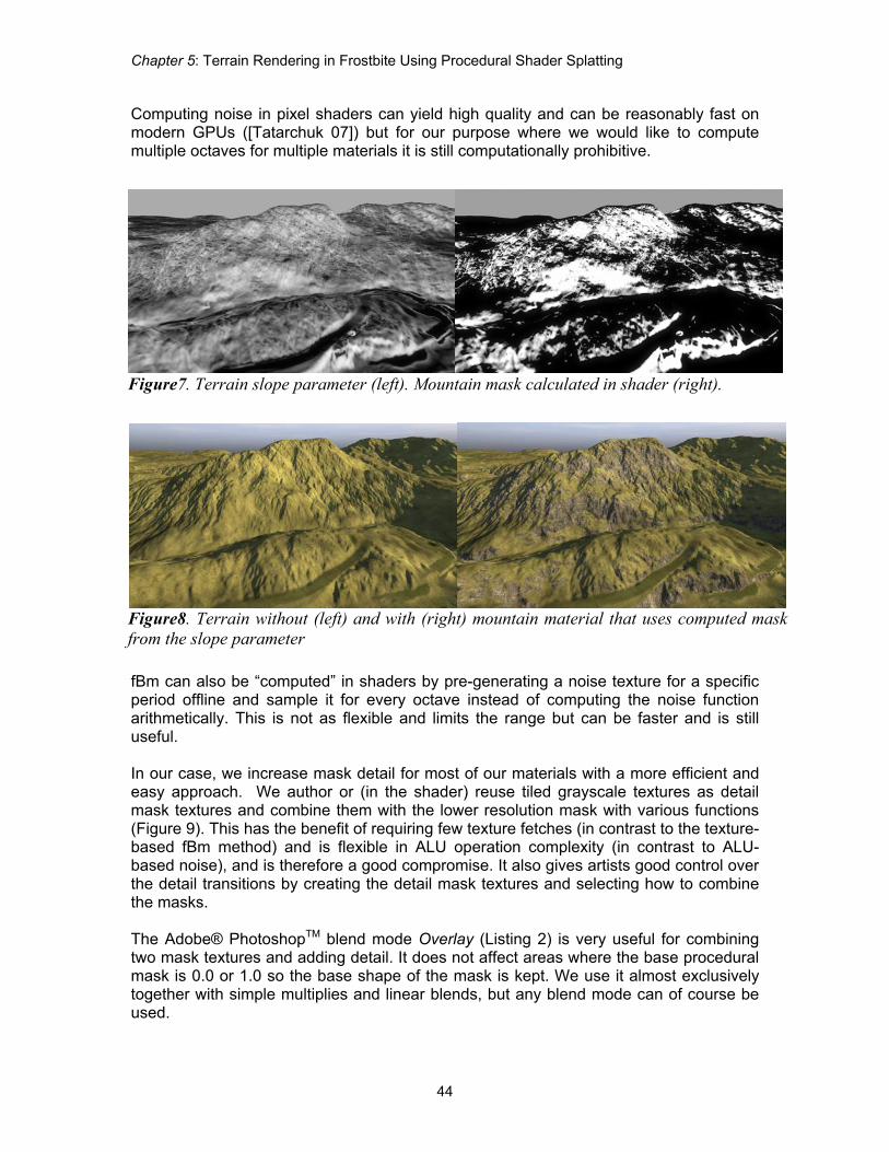
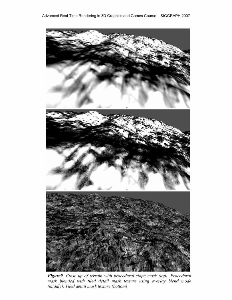
fBm can also be “computed” in shaders by pre-generating a noise texture for a specific period offline and sample it for every octave instead of computing the noise function arithmetically. This is not as flexible and limits the range but can be faster and is still useful. In our case, we increase mask detail for most of our materials with a more efficient and easy approach. We author or (in the shader) reuse tiled grayscale textures as detail mask textures and combine them with the lower resolution mask with various functions (Figure 9). This has the benefit of requiring few texture fetches (in contrast to the texture-based fBm method) and is flexible in ALU operation complexity (in contrast to ALU-based noise), and is therefore a good compromise. It also gives artists good control over the detail transitions by creating the detail mask textures and selecting how to combine the masks. The Adobe® PhotoshopTM blend mode Overlay (Listing 2) is very useful for combining two mask textures and adding detail. It does not affect areas where the base procedural mask is 0.0 or 1.0 so the base shape of the mask is kept. We use it almost exclusively together with simple multiplies and linear blends, but any blend mode can of course be used.
Figure8. Terrain without (left) and with (right) mountain material that uses computed mask from the slope parameter
Advanced Real-Time Rendering in 3D Graphics and Games Course – SIGGRAPH 2007
45
Figure9. Close up of terrain with procedural slope mask (top). Procedural mask blended with tiled detail mask texture using overlay blend mode (middle). Tiled detail mask texture (bottom)
Chapter 5: Terrain Rendering in Frostbite Using Procedural Shader Splatting
46
Having multiple detail mask textures together with all other textures quickly eat performance and texture samplers (only 16 are available in Shader Model 3). To improve on this, we have had some good results with reusing channels of ordinary color textures, or even normal maps, already used in the shader, potentially with different tiling of the texture coordinates, and remapping the range or changing the contrast (Listing 2) to get a normalized mask value and use that instead of an extra texture.
Listing 2. Overlay blend and contrast HLSL functions. Works with values in normalized [0, 1] range and can be easily extended for arbitrary dimensions (colors for example).
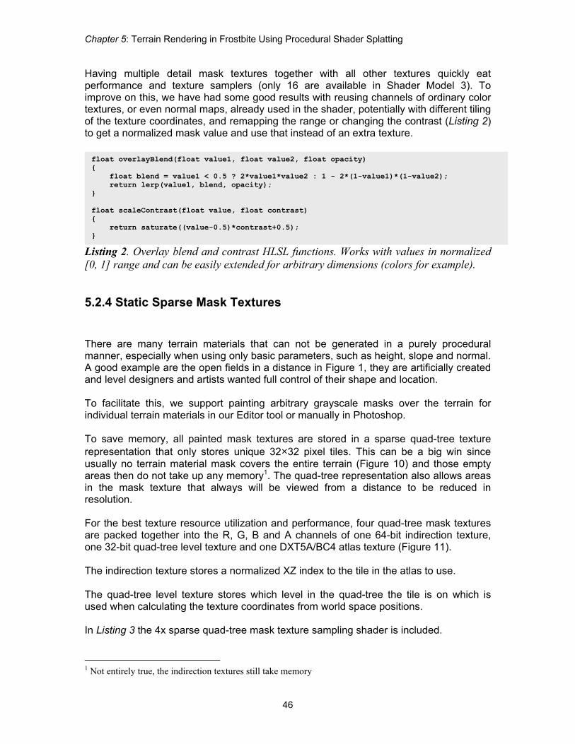
5.2.4 Static Sparse Mask Textures There are many terrain materials that can not be generated in a purely procedural manner, especially when using only basic parameters, such as height, slope and normal. A good example are the open fields in a distance in Figure 1, they are artificially created and level designers and artists wanted full control of their shape and location. To facilitate this, we support painting arbitrary grayscale masks over the terrain for individual terrain materials in our Editor tool or manually in Photoshop. To save memory, all painted mask textures are stored in a sparse quad-tree texture representation that only stores unique 32×32 pixel tiles. This can be a big win since usually no terrain material mask covers the entire terrain (Figure 10) and those empty areas then do not take up any memory1. The quad-tree representation also allows areas in the mask texture that always will be viewed from a distance to be reduced in resolution. For the best texture resource utilization and performance, four quad-tree mask textures are packed together into the R, G, B and A channels of one 64-bit indirection texture, one 32-bit quad-tree level texture and one DXT5A/BC4 atlas texture (Figure 11). The indirection texture stores a normalized XZ index to the tile in the atlas to use. The quad-tree level texture stores which level in the quad-tree the tile is on which is used when calculating the texture coordinates from world space positions. In Listing 3 the 4x sparse quad-tree mask texture sampling shader is included. 1 Not entirely true, the indirection textures still take memory
Advanced Real-Time Rendering in 3D Graphics and Games Course – SIGGRAPH 2007
47
When creating and sampling from the mask texture atlas, care must be taken to pad the borders of the tiles to prevent filtering artifacts in the edges when bilinear filtering is used. Otherwise parts of the bordering tile in the atlas will leak over in the edges resulting in ugly line artifacts in the borders of the tiles. In Direct3D10 and on Xbox 360, a texture array can be used instead of an atlas and then bilinear filtering automatically works correctly without any extra padding. Unfortunately texture arrays have a limit of 512 slices (tiles) in Direct3D10 and 64 slices on Xbox 360 which limits their usefulness in this case unless the tiles are split up over multiple texture arrays.
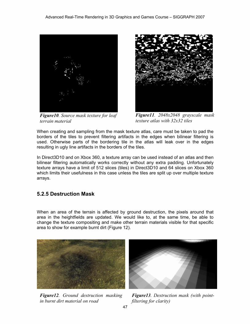
5.2.5 Destruction Mask When an area of the terrain is affected by ground destruction, the pixels around that area in the heightfields are updated. We would like to, at the same time, be able to change the texture compositing and make other terrain materials visible for that specific area to show for example burnt dirt (Figure 12).
Figure11. 2048x2048 grayscale mask texture atlas with 32x32 tiles
Figure10. Source mask texture for leaf terrain material
Figure12. Ground destruction masking in burnt dirt material on road
Figure13. Destruction mask (with point-filtering for clarity)
Chapter 5: Terrain Rendering in Frostbite Using Procedural Shader Splatting
48
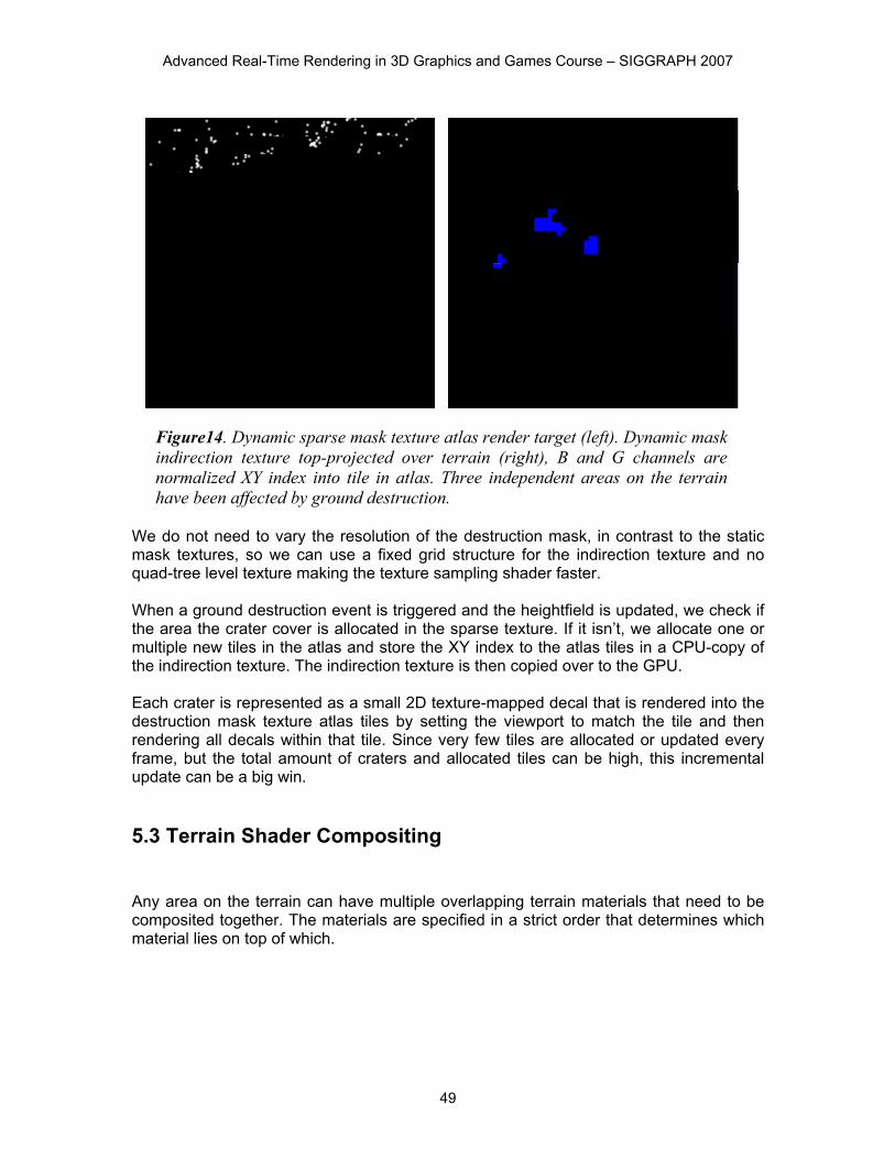
Listing 3. Quad-tree texture sampling shader (Direct3D 10 HLSL), output is 4 individual mask values. Note: padding between tiles is not included. We do this by dynamically rendering textured mask decals into a unique destruction mask texture that covers the entire terrain that can be destructed (Figure 13). The destruction mask is very low resolution, 4 pixels per meter, because the mask only needs to contain rough circular gradients in the areas affected by ground destruction. More detail can be added in the shaders in a similar manner of adding detail to the procedural masks and the painted mask textures we described earlier in this chapter. Nonetheless, even with a reasonably low resolution, texture memory footprint becomes a problem. In a 2048×2048 m destructible terrain area, a 4 pixel per meter uncompressed 8-bit mask texture takes (2048 * 4)2 bytes = 64 MB. That is hardly desirable on any platform. In our case, the worst case scenario for ground destruction is not really that 100% of the terrain area can be fully destroyed and need to be masked at the same time. The percentage we can get away with is much lower, perhaps 10%. But we do not want to restrict where on the terrain the destruction can happen, so the 10% destroyed area can be arbitrarily scattered over the entire terrain. This is a similar scenario to static sparse mask textures that we encountered before, however with dynamic textures in this case. So what we chose to do to save memory is to create and incrementally update a dynamic sparse mask texture on the GPU for the ground destruction (Figure 14).
Advanced Real-Time Rendering in 3D Graphics and Games Course – SIGGRAPH 2007
49
We do not need to vary the resolution of the destruction mask, in contrast to the static mask textures, so we can use a fixed grid structure for the indirection texture and no quad-tree level texture making the texture sampling shader faster. When a ground destruction event is triggered and the heightfield is updated, we check if the area the crater cover is allocated in the sparse texture. If it isn’t, we allocate one or multiple new tiles in the atlas and store the XY index to the atlas tiles in a CPU-copy of the indirection texture. The indirection texture is then copied over to the GPU. Each crater is represented as a small 2D texture-mapped decal that is rendered into the destruction mask texture atlas tiles by setting the viewport to match the tile and then rendering all decals within that tile. Since very few tiles are allocated or updated every frame, but the total amount of craters and allocated tiles can be high, this incremental update can be a big win.
5.3 Terrain Shader Compositing Any area on the terrain can have multiple overlapping terrain materials that need to be composited together. The materials are specified in a strict order that determines which material lies on top of which.
Figure14. Dynamic sparse mask texture atlas render target (left). Dynamic mask indirection texture top-projected over terrain (right), B and G channels are normalized XY index into tile in atlas. Three independent areas on the terrain have been affected by ground destruction.
Chapter 5: Terrain Rendering in Frostbite Using Procedural Shader Splatting
50
A simple implementation to render the materials would be to do the compositing of the terrain materials in the frame buffer using alpha-blending a la [Bloom00]. Such an implementation would go through each terrain material in back-to-front order and render all terrain geometry associated with that material and blending its output on top of the previous material’s output. However there are quite a few drawbacks with such a multi-pass approach:
x Frame buffer bandwidth. The terrain covers much of the screen and the more materials we add the more times every pixel has to be read and written back to the frame buffer costing memory bandwidth.
x Geometry overdraw. As with any multi-pass technique, the geometry is rendered multiple times. Since we want to render the terrain with lots of triangles for good detail and GPU vertex throughput isn’t increasing as fast as pixel throughput, this can become a big bottleneck.
x Duplicated shader computation. Many of the computations in the terrain material shaders such as the terrain normal would be recomputed for every pass which is costly.
x Fixed function blend modes. The built-in blend modes aren’t very flexible, especially compared to shaders. There are lots of interesting methods to non-linearly combine natural textures for terrain
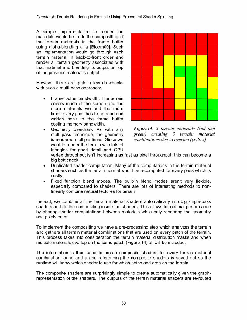
Instead, we combine all the terrain material shaders automatically into big single-pass shaders and do the compositing inside the shaders. This allows for optimal performance by sharing shader computations between materials while only rendering the geometry and pixels once. To implement the compositing we have a pre-processing step which analyzes the terrain and gathers all terrain material combinations that are used on every patch of the terrain. This process takes into consideration the terrain material distribution masks and when multiple materials overlap on the same patch (Figure 14) all will be included. The information is then used to create composite shaders for every terrain material combination found and a grid referencing the composite shaders is saved out so the runtime will know which shader to use for which patch and area on the terrain. The composite shaders are surprisingly simple to create automatically given the graph-representation of the shaders. The outputs of the terrain material shaders are re-routed
Figure14. 2 terrain materials (red and green) creating 3 terrain material combinations due to overlap (yellow)
Advanced Real-Time Rendering in 3D Graphics and Games Course – SIGGRAPH 2007
51
to the inputs of a pre-created compositing shader that combines all the materials and outputs the final color. Duplicate resources (textures, samplers and constants) and identical graph sub-trees or code in the composite shaders are automatically removed by the general shader graph compiler.
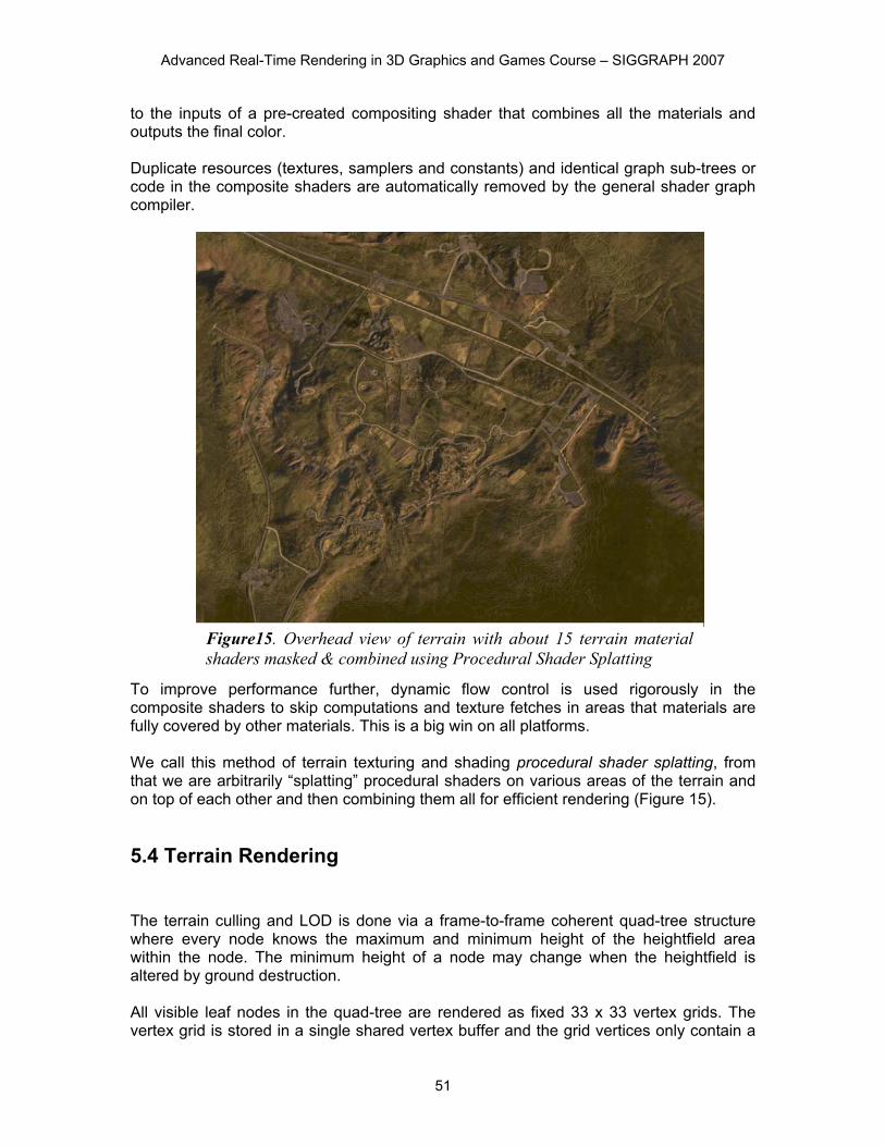
To improve performance further, dynamic flow control is used rigorously in the composite shaders to skip computations and texture fetches in areas that materials are fully covered by other materials. This is a big win on all platforms. We call this method of terrain texturing and shading procedural shader splatting, from that we are arbitrarily “splatting” procedural shaders on various areas of the terrain and on top of each other and then combining them all for efficient rendering (Figure 15).
5.4 Terrain Rendering The terrain culling and LOD is done via a frame-to-frame coherent quad-tree structure where every node knows the maximum and minimum height of the heightfield area within the node. The minimum height of a node may change when the heightfield is altered by ground destruction. All visible leaf nodes in the quad-tree are rendered as fixed 33 x 33 vertex grids. The vertex grid is stored in a single shared vertex buffer and the grid vertices only contain a
Figure15. Overhead view of terrain with about 15 terrain material shaders masked & combined using Procedural Shader Splatting
Chapter 5: Terrain Rendering in Frostbite Using Procedural Shader Splatting
52
4-byte UV coordinate that gives a [0,1] parameterization over the grid. This parameterization is transformed into both heightfield- and world-space in the vertex shader and used for fetching the terrain height for the vertex trough the heightfield texture. Because the vertex grid is aligned with the heightfield, point-filtering can be used which is a benefit on GPUs that does not natively support bilinear filtering of textures in vertex shaders (GeForce 6 and 7). On platforms and graphics cards that do not efficiently support vertex texture fetch we have a pool of 33×33 vertices vertex buffers that are allocated on-demand on a LRU-basis to visible quad tree nodes and filled by CPU/SPU threads by sampling the heightfield. The fixed vertex grid resolution is important to be able to support the worst case scenario with arbitrary ground destruction at a fixed cost and quality. This “wastes” triangles in non-altered flat areas but we found the cost to be worthwhile because of the simplicity and generality of this approach.
5.4.1 Geometry LOD
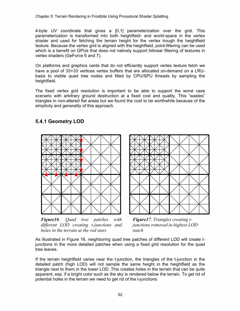
As illustrated in Figure 16, neighboring quad tree patches of different LOD will create t-junctions in the more detailed patches when using a fixed grid resolution for the quad tree leaves. If the terrain heightfield varies near the t-junction, the triangles of the t-junction in the detailed patch (high LOD) will not sample the same height in the heightfield as the triangle next to them in the lower LOD. This creates holes in the terrain that can be quite apparent, esp. if a bright color such as the sky is rendered below the terrain. To get rid of potential holes in the terrain we need to get rid of the t-junctions.
Figure17. Triangles creating t-junctions removed in highest LOD patch
Figure16. Quad tree patches with different LOD creating t-junctions and holes in the terrain at the red stars
Advanced Real-Time Rendering in 3D Graphics and Games Course – SIGGRAPH 2007
53
We can do this by first requiring that all quad tree nodes have a maximum of 1 level difference to its neighbors. Then replace the two triangles that make up every t-junction in the detailed patch with a single triangle that only uses vertices also available in the neighboring lower LOD (Figure 17). These vertices are guaranteed to exist by the max level difference we required. To support all possible combinations of quad tree nodes with the max level difference restriction, all we need are 9 different index buffer permutations (Figure 18):
x One permutation that has all triangles in the vertex grid intact and is used when the neighbor patches are of the same level. This is the most common case.
x Four permutations with the t-junction triangles removed on one of the four sides of the patch
x Four permutations with the t-junction triangles removed on two sides next to each other
x The reason why we do not need all possible sixteen permutations (t-junctions from all sides individually removed or kept) is that we chose to remove geometry from the detailed patches instead of adding geometry to the lower LOD patches (which also works). Two sides of a quad tree leaf node always shares the parent, and thus LOD, which means that we do not need to remove t-junctions from more than two sides next to each other of a patch. This technique with multiple index buffer permutations is a bit similar to [Dallaire06], but working with quad-trees instead of same size patches.
Figure18. The 9 geometry permutations needed for t-junction free LOD transitions
Chapter 5: Terrain Rendering in Frostbite Using Procedural Shader Splatting
54
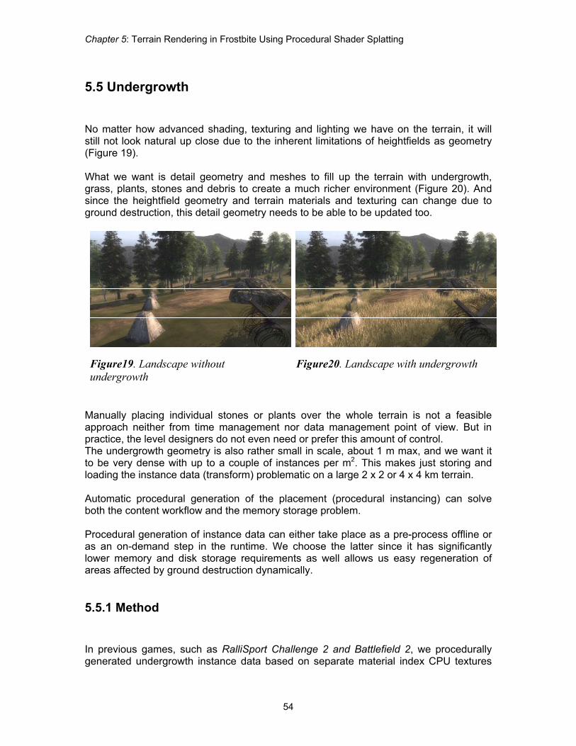
5.5 Undergrowth No matter how advanced shading, texturing and lighting we have on the terrain, it will still not look natural up close due to the inherent limitations of heightfields as geometry (Figure 19). What we want is detail geometry and meshes to fill up the terrain with undergrowth, grass, plants, stones and debris to create a much richer environment (Figure 20). And since the heightfield geometry and terrain materials and texturing can change due to ground destruction, this detail geometry needs to be able to be updated too.
Figure19. Landscape without undergrowth
Figure20. Landscape with undergrowth
Manually placing individual stones or plants over the whole terrain is not a feasible approach neither from time management nor data management point of view. But in practice, the level designers do not even need or prefer this amount of control. The undergrowth geometry is also rather small in scale, about 1 m max, and we want it to be very dense with up to a couple of instances per m2. This makes just storing and loading the instance data (transform) problematic on a large 2 x 2 or 4 x 4 km terrain. Automatic procedural generation of the placement (procedural instancing) can solve both the content workflow and the memory storage problem. Procedural generation of instance data can either take place as a pre-process offline or as an on-demand step in the runtime. We choose the latter since it has significantly lower memory and disk storage requirements as well allows us easy regeneration of areas affected by ground destruction dynamically.
5.5.1 Method In previous games, such as RalliSport Challenge 2 and Battlefield 2, we procedurally generated undergrowth instance data based on separate material index CPU textures
Advanced Real-Time Rendering in 3D Graphics and Games Course – SIGGRAPH 2007
55
top-projected on the terrain. These maps indexed artist-defined undergrowth materials that contained distribution settings such as which meshes to distribute, density (amount per m2), random scale range, animation settings, etc. The system worked well but there were three main limitations with the material index maps that we wanted to resolve in Frostbite:
x Undergrowth materials can not overlap. Painting an area with a different type of undergrowth is cumbersome and limited since you need to clone the material that was already there, and in the material add the new types of geometry to distribute.
x Undergrowth materials are fully separate from the underlying terrain materials. If the terrain textures were repainted to be dirt instead of grass in an area, the undergrowth material index map would have to be repainted manually as well.
x Resolution and destruction. With dynamic ground destruction we need to have a much higher resolution of these textures costing memory.
As we now texture, shade and distribute terrain materials and textures through shaders it felt natural to use the same system of procedural shader splatting for the undergrowth generation. Then all the already existing terrain materials could automatically have undergrowth distributed in their specific areas with minimal work on content. Ground destruction and overlapping materials are also already a part of the general terrain material masking so it is a very good fit.
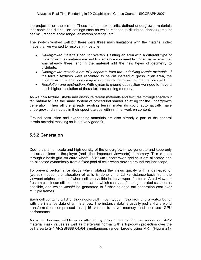
5.5.2 Generation Due to the small scale and high density of the undergrowth, we generate and keep only the areas close to the player (and other important viewports) in memory. This is done through a basic grid structure where 16 x 16m undergrowth grid cells are allocated and de-allocated dynamically from a fixed pool of cells when moving around the landscape. To prevent performance drops when rotating the views quickly with a gamepad or (worse) mouse; the allocation of cells is done on a 2d xz distance-basis from the viewport origins instead of when cells are visible in the viewport frustums. A cell viewport frustum check can still be used to separate which cells need to be generated as soon as possible, and which should be generated to further balance out generation cost over multiple frames. Each cell contains a list of the undergrowth mesh types in the area and a vertex buffer with the instance data of all instances. The instance data is usually just a 4 x 3 world transformation compressed as fp16 values to save memory and increase GPU performance. As a cell become visible or is affected by ground destruction, we render out 4-12 material mask values as well as the terrain normal with a top-down projection over the cell area to 2-4 ARGB8888 64x64 simultaneous render targets using MRT (Figure 21).
Chapter 5: Terrain Rendering in Frostbite Using Procedural Shader Splatting
56
The shader used is automatically generated offline in a similar manner to the terrain shader compositing shaders.
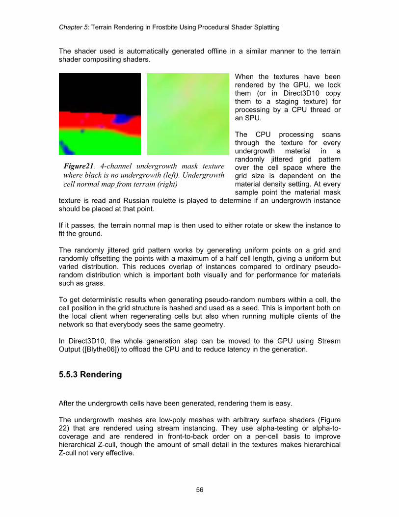
When the textures have been rendered by the GPU, we lock them (or in Direct3D10 copy them to a staging texture) for processing by a CPU thread or an SPU. The CPU processing scans through the texture for every undergrowth material in a randomly jittered grid pattern over the cell space where the grid size is dependent on the material density setting. At every sample point the material mask
texture is read and Russian roulette is played to determine if an undergrowth instance should be placed at that point. If it passes, the terrain normal map is then used to either rotate or skew the instance to fit the ground. The randomly jittered grid pattern works by generating uniform points on a grid and randomly offsetting the points with a maximum of a half cell length, giving a uniform but varied distribution. This reduces overlap of instances compared to ordinary pseudo-random distribution which is important both visually and for performance for materials such as grass. To get deterministic results when generating pseudo-random numbers within a cell, the cell position in the grid structure is hashed and used as a seed. This is important both on the local client when regenerating cells but also when running multiple clients of the network so that everybody sees the same geometry. In Direct3D10, the whole generation step can be moved to the GPU using Stream Output ([Blythe06]) to offload the CPU and to reduce latency in the generation.
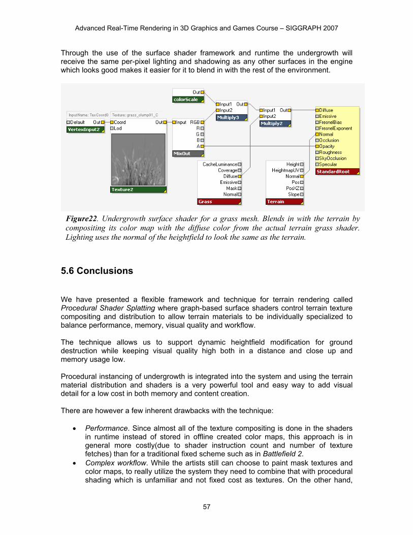
5.5.3 Rendering After the undergrowth cells have been generated, rendering them is easy. The undergrowth meshes are low-poly meshes with arbitrary surface shaders (Figure 22) that are rendered using stream instancing. They use alpha-testing or alpha-to-coverage and are rendered in front-to-back order on a per-cell basis to improve hierarchical Z-cull, though the amount of small detail in the textures makes hierarchical Z-cull not very effective.
Figure21. 4-channel undergrowth mask texture where black is no undergrowth (left). Undergrowth cell normal map from terrain (right)
Advanced Real-Time Rendering in 3D Graphics and Games Course – SIGGRAPH 2007
57
Through the use of the surface shader framework and runtime the undergrowth will receive the same per-pixel lighting and shadowing as any other surfaces in the engine which looks good makes it easier for it to blend in with the rest of the environment.
5.6 Conclusions We have presented a flexible framework and technique for terrain rendering called Procedural Shader Splatting where graph-based surface shaders control terrain texture compositing and distribution to allow terrain materials to be individually specialized to balance performance, memory, visual quality and workflow. The technique allows us to support dynamic heightfield modification for ground destruction while keeping visual quality high both in a distance and close up and memory usage low. Procedural instancing of undergrowth is integrated into the system and using the terrain material distribution and shaders is a very powerful tool and easy way to add visual detail for a low cost in both memory and content creation. There are however a few inherent drawbacks with the technique:
x Performance. Since almost all of the texture compositing is done in the shaders
in runtime instead of stored in offline created color maps, this approach is in general more costly(due to shader instruction count and number of texture fetches) than for a traditional fixed scheme such as in Battlefield 2.
x Complex workflow. While the artists still can choose to paint mask textures and color maps, to really utilize the system they need to combine that with procedural shading which is unfamiliar and not fixed cost as textures. On the other hand,
Figure22. Undergrowth surface shader for a grass mesh. Blends in with the terrain by compositing its color map with the diffuse color from the actual terrain grass shader. Lighting uses the normal of the heightfield to look the same as the terrain.
Chapter 5: Terrain Rendering in Frostbite Using Procedural Shader Splatting
58
procedural elements can be more easily shared and reused across multiple terrains.
The flexibility built into the technique and framework makes it a great scaleable platform to integrate interesting shading techniques and texturing schemes in the future. 5.7 References [AT07] ANDERSSON, J., TATARCHUK, N. 2007. Frostbite Rendering Architecture and Real-
time Procedural Shading and Texturing Techniques. AMD Sponsored Session. GDC 2007. March 5-9, 2007, San Francisco, CA. http://ati.amd.com/developer/gdc/2007/Andersson-Tatarchuk-FrostbiteRenderingArchitecture(GDC07_AMD_Session).pdf
[BLOOM00] BLOOM, C. 2000. Terrain Texture Compositing by Blending in the Frame-Buffer
(a.k.a. "Splatting" Textures). Nov 2, 2000. http://www.cbloom.com/3d/techdocs/splatting.txt [BLYTHE06] BLYTHE, D. 2006. The Direct3D 10 system. In proceedings of ACM
Transactions on Graphics (SIGGRAPH’06 Conference Proceedings), pp. 724-234, Boston, Massachusetts.
[DALLAIRE06] DALLAIRE, C. 2006. Binary Triangle Trees for Terrain Tile Index Buffer
Generation. Gamasutra article. http://www.gamasutra.com/features/20061221/dallaire_01.shtml [TATARCHUK06] TATARCHUK, N. 2006. Dynamic parallax occlusion mapping with
approximate soft shadows. In proceedings of AMD SIGGRAPH Symposium on Interactive 3D Graphics and Games, pp. 63-69, Redwood City, CA.
[TATARCHUK07] TATARCHUK, N. 2007. The Importance of Being Noisy: Fast, High Quality
Noise. Conference Session. GDC 2007. March 5-9, 2007, San Francisco, CA. http://ati.amd.com/developer/gdc/2007/Tatarchuk-Noise(GDC07-D3D_Day).pdf
[TERRAGEN*] TERRAGEN by Planetside Software. http://www.planetside.co.uk/terragen/ [WEi04] WEI, L. 2004. Tile-Based Texture Mapping on Graphics Hardware. In
proceedings of ACM SIGGRAPH/Eurographics conference on Graphics Hardware, pp. 55-63. Grenoble, France.