Checking for normality in linear mixed models

SCIENCE CHINAMathematics

. ARTICLES . April 2012 Vol. 55 No. 4: 787–804

doi: 10.1007/s11425-011-4352-0

c© Science China Press and Springer-Verlag Berlin Heidelberg 2012 math.scichina.com www.springerlink.com

Checking for normality in linear mixed models

WU Ping1,∗, ZHU LiXing2,3 & FANG Yun4

1School of Finance and Statistics, East China Normal University, Shanghai 200241, China;2School of Statistics and Mathematics, Yunnan University of Finance and Economics, Yunnan 650221, China;

3The Department of Mathematics, Hong Kong Baptist University, Hong Kong 999077, China;4Mathematics and Science College, Shanghai Normal University, Shanghai 200234, China

Email: [email protected], [email protected], [email protected]

Received August 20, 2010; accepted May 22, 2011; published online January 9, 2012

Abstract Linear mixed models are popularly used to fit continuous longitudinal data, and the random effects

are commonly assumed to have normal distribution. However, this assumption needs to be tested so that further

analysis can be proceeded well. In this paper, we consider the Baringhaus-Henze-Epps-Pulley (BHEP) tests,

which are based on an empirical characteristic function. Differing from their case, we consider the normality

checking for the random effects which are unobservable and the test should be based on their predictors. The

test is consistent against global alternatives, and is sensitive to the local alternatives converging to the null at

a certain rate arbitrarily close to 1/√n where n is sample size. Furthermore, to overcome the problem that the

limiting null distribution of the test is not tractable, we suggest a new method: use a conditional Monte Carlo

test (CMCT) to approximate the null distribution, and then to simulate p-values. The test is compared with

existing methods, the power is examined, and several examples are applied to illustrate the usefulness of our

test in the analysis of longitudinal data.

Keywords linear mixed models, estimated best linear unbiased predictors, BHEP tests, conditional Monte

Carlo test

MSC(2010) 62G10, 62E20

Citation: Wu P, Zhu L X, Fang Y. Checking for normality in linear mixed models. Sci China Math, 2012, 55(4):

787–804, doi: 10.1007/s11425-011-4352-0

1 Introduction

To analyze continuous longitudinal data, linear mixed models have been applied frequently. A commonly

used assumption is that the random effects as well as the error terms follow normal distributions, or more

generally, parametric distributions, see, e.g., [7, 8, 14]. The importance of the normality of random effects

has been extensively investigated in the literature, please see [10, 16, 17, 22, 25, 26]. Testing normality

for mixed models has attracted much attention from statisticians, for example [2, 11].

Since the random effects are not observable, the distributional properties of the predicted random

effects, say the estimated best linear unbiased predictions (EBLUPs) become critical inferring tools. [15]

proposed using weighted normal plots by comparing the expected and the empirical cumulative func-

tions of the standardized linear combination of EBLUPs to check various departures from the normality

assumption. For one-level random effects, [21] extended the pointwise result of [15] to a result for a

weighted empirical process, and constructed a test that is based on the difference between a weighted

empirical distribution function of the standardized EBLUPs and its expectation. Inspired by [21], [28]

∗Corresponding author

788 Wu P et al. Sci China Math April 2012 Vol. 55 No. 4

recommended analogous tests that are based on the simulating samples from the random effects’ posterior

distribution with estimated parameters. His method applies to generalized linear mixed models but the

random effects must be one level as well. Similar statistical inference was also considered by [11] who

developed Pearson’s χ2-statistics for more general distributional assumptions. In addition, [27] proposed

to check the normality of the random effects using gradient function.

When the random effects are multivariate, besides the diagnostic plots in [15], [2] proposed several tests

including the order-selection tests (OS tests) and the minimum distance tests to check the normality of

the random effects and error separately and simultaneously. However, the power of the order selection

tests was not so good (see [19]). Moreover, people should be careful to use other criteria for the order

selection, such as BIC (see [3, 12]). Also, just like [15], [2] did not investigate the asymptotic behavior of

the tests.

In this paper, we consider linear mixed models where the observations are divided into independent

groups with one random effect (or vector of the random effects) corresponding to each group, and then

propose a test procedure to check the normality assumption for the random effects, regardless of whether

they are univariate or multidimensional. Based on an empirical characteristic function, the BHEP test

for assessing univariate and multivariate normality were introduced by [1] and [5] respectively. Here we

extend the BHEP tests for multivariate normality of [9] and construct a test statistic that is based on a

weighted integral of the squared modulus of the difference between the empirical characteristic function

of the scaled ones of the standardized EBLUPs and its almost sure pointwise limit exp{− ‖t‖2

2 } under

the normality hypothesis H0. As commented by [9], this test statistic can be interpreted alternatively in

terms of the L2-distance between a nonparametric kernel density estimator and the parametric density

estimator if H0 is true. Moreover, the test shares some desired features.

1. It is feasible for the random effects of any dimension.

2. We investigate in detail the power performance theoretically. The test is consistent against global

alternatives, and is even sensitive to contiguous alternatives converging to the null at the rate n−1/2, the

fastest possible rate for goodness-of-fit testing.

3. Because model parameters need to be estimated, the test is not asymptotically distribution-free.

This is also the case for all existing tests. A new Monte Carlo method—the conditional Monte Carlo

test (CMCT)— is proposed to simulate the null distribution and p-values. Rather than simulating the

limit Gaussian process as [21] did, we directly simulate the reference data that come from a distribution

from which, under the null hypothesis, the original data come. Thus, it has better performance in finite

sample cases.

This article is organized as follows. In Section 2, we briefly introduce linear mixed models and give

some notations. In Section 3, we describe the method and our main results. The CMCT is reported in

Section 4. Section 5 includes simulation studies and applications in several practical examples. Finally,

all proofs are given in the appendix.

2 Linear mixed models and notations

Consider the model

Yi = Xiβ + Zibi + εi, i = 1, . . . , n, (1)

where Yi is the li × 1 vector of responses for the ith individual, Xi and Zi are, respectively, known,

nonrandom between-individuals and within-individuals design matrices of li × p and li × q for the fixed

effects β and random effects bi, and εi is the ith error term of li×1. Obviously β is a p×1 unknown vector,

and bi is a random vector of q×1. Usually one assumes that the εis ∼ind N (0, σ2Ili) and are independent

of the bis ∼iid Nq(0, D), where σ2 is the unknown variance of the εis, D = D(δ) is a positive-definite

covariance matrix and is known up to the parameter vector δ of k×1, and Ili is an li× li identity matrix.

For the case of model identifiability, moreover, we assume li > q for some i. Here and throughout the

paper i.i.d. means independent and identically distributed and i.n.d. independent but nonidentically

Wu P et al. Sci China Math April 2012 Vol. 55 No. 4 789

distributed. Usually δ includes all of the unknown elements of D, and then D is a smooth function of δ.

Without confusion, we assume that D is differentiable about δ throughout this paper. Obviously the

marginal distribution of Yi is normal with mean Xiβ and covariance matrix

Vi = Vi(α) = σ2Ili + ZiD(δ)Z ′i, (2)

where A′ denotes the transpose of A for any vector or matrix A and α = (σ2, δ′)′ of (k + 1) × 1. In a

degree, the popularity of model (1) is due to the attractive and often appropriate linear pattern (2) for

the covariance structure of Yi. Let θ = (α′, β′)′ denote all of the parameters in the marginal distribution

and Θ ⊆ Rp+k+1 the corresponding parameter space. The log likelihood for θ except some constants not

depending on θ is

L(θ) =

n∑

i=1

Li(θ) = −1

2

n∑

i=1

log(|Vi(α)|) − 1

2

n∑

i=1

(Yi −Xiβ)′Vi(α)

−1(Yi −Xiβ), (3)

where V −1i is the inverse matrix and this notation is used throughout this paper. Then the maximum

likelihood estimator (MLE) of θ, denoted by θ, is the solution to Q(θ) = 0, where

Q(θ) =∂L(θ)

∂θ=

n∑

i=1

Qi(Yi −Xiβ; θ), (4)

and Qi involves only the observations from the ith individual with zero mean and a positive-definite

covariance. Let the true parameter value θ0 = (σ20 , δ

′0, β0)

′ lies within the interior of the set Θ. Under

the normality assumption,

n1/2(θ − θ0) = Ω−1n−1/2n∑

i=1

Qi(Yi −Xiβ0; θ0) + op(1), (5)

where Ω = limn→∞ Σn(θ0), and Σn(θ0) = −n−1∂2L(θ0)/∂θ∂θ′. n1/2(θ − θ0) converges to a zero-mean

Gaussian variable V with covariance matrix Ω−1 and Ω−1 can be consistently estimated by A−1n defined

below. Refer to [18] for details. Moreover, [10] showed that the MLE θ is still consistent and asymptoti-

cally normally distributed even when the random-effects distribution is not normal, but a sandwich-type

correction to the inverse Fisher information matrix is then needed in order to get the correct asymptotic

covariance matrix. The corrected estimate of Ω−1 is A−1n BnA

−1n /n, where

An = − 1

n

n∑

i=1

∂2Li(θ)

∂θ∂θ′, Bn =

1

n

n∑

i=1

∂Li(θ)

∂θ

∂Li(θ)

∂θ′.

For any fixed θ ∈ Θ, the best linear unbiased predictions (BLUPs) under normal hypothesis, are the

corresponding posterior expectations of the bis,

bi = bi(θ) = D(δ)Z ′iV

−1i (α)(Yi −Xiβ), i = 1, . . . , n. (6)

See, for example, [14] for a derivation of expression (6). Then the BLUPs bis ∼ind N (0,Wi), where

Wi = Wi(θ) = D(δ)Z ′iV

−1i (α)ZiD(δ) (i = 1, . . . , n). Replacing δ by its estimator, we obtain the estimator

D = D(δ) of D. Similarly Vi, Wi and bi(θ) are defined. For notational simplicity, we also denote by D0,

Vi0 and Wi0 the corresponding matrices under the true parameter θ0. The estimators of the BLUPs,

bi(θ) = DZ ′iV

−1i (Yi −Xiβ), i = 1, . . . , n,

are referred to as EBLUPs, and they are approximately normally distributed.


3 The construction of test

In this paper, we assume that error εis have a zero-mean multivariate Gaussian distribution, and just

check whether the random effect bis are normal. As commented by [15], [21] and others, the distribution

of bi depends not only on the distribution of bi but also on that of εi. Then the BLUPs are not normally

distributed if the distribution of either the random effects or the individual errors are not normal, so that

testing the normality on both bi and εi is equivalently testing normality of the BLUPs.

H0 : The BLUPs are normally distributed.

From the above remarks, H0 indicates that both bi and εi are normal, whereas rejection of H0 means

that at least one of them is not. In the following section, we construct a test statistic.

3.1 The BHEP test for multivariate normality

We first give some notations. From (6), the standardized BLUPs are denoted by

ui = ui(θ) = W−1/2i DZ ′

iV−1i (Yi −Xiβ), i = 1, . . . , n, (7)

where W1/2i is the square root decomposition of Wi. The standardized EBLUPs are denoted by un1 =

u1(θ), . . . , unn = un(θ), and u01 = u1(θ0), . . . , u0n = un(θ0) denote the values of the standardized BLUPs

under the true parameter θ0. We denote the empirical covariance matrix of u1, . . . , un by Sn(θ) =

n−1∑n

i=1(ui − un)(ui − un)′, where un = n−1

∑ni=1 ui. The corresponding scaled ui is denoted by

Ui(θ) = S−1/2n (ui − un). Replacing θ by θ, the empirical covariance matrix of un1, . . . , unn is expressed

by Snn = Sn(θ) with unn = un(θ). Similarly we define Uni = Ui(θ), U0i = Ui(θ0), S0n = Sn(θ0), and

u0n = un(θ0). Of course, the later three are obtained when inserting the true parameter θ0. Under model

(1), the u0is ∼iid Nq(0, Iq), and the unis are the consistent estimators of the BLUPs (under the true

parameters).

Because the BLUPs depend on unknown parameters, we then use the EBLUPs to construct the test.

Following [9], we define the distance between the empirical characteristic type function of the Unis and

its almost sure point-wise limit exp{− ‖t‖2

2 } under the true parameter distribution as

Gn(t) =1

n

n∑

i=1

[cos(t′Uni) + sin(t′Uni)− exp

{− ‖t‖2

2

}], (8)

that is a random element in the Frechet space C(Rq) of continuous functions on Rq, endowed with the

metric

ρ(x, y) =∞∑

k=1

2−k ρk(x, y)

1 + ρk(x, y),

where

ρk(x, y) = max‖t‖�k

|x(t) − y(t)| .

Consider the following test statistic

Tn,γ = n

∫

Rq

G2n(t)ϕγ(t)dt, (9)

where the weight function ϕγ(t) = (2πγ)−q/2 exp{− ‖t‖2

2γ2 }. We should reject the null hypothesis H0 for

large values of Tn,γ .

Substituting U0i for Uni in (8), we obtain the process Gn0(t) which was used to test whether or not a

random variable or vector is normal by [9], and they showed that Gn0(t) converges in distribution to a

centered Gaussian process G0(t) in C(Rq) with covariance kernel

K0(s, t) = exp

{− ‖s− t‖2

2

}−(1 + s′t+

(s′t)2

2

)exp

{− ‖s‖2 + ‖t‖2

2

}, s, t ∈ Rq, (10)


and their test statistic n∫Rq G

2n(t)ϕγ(t)dt converges to

∫Rq G

20(t)ϕγ(t)dt in distribution. However, our

situation is more complicated because of the use of estimators for the unknowns to obtain the Unis. Before

we present the asymptotic behavior of Gn(t), we first note that [10] proved the strong consistency and

the asymptotic normality of θ under fairly general regularity conditions on the parameter space and on

the covariances X and Z. As [10] pointed out, the conditions also involve the unknown correct random-

effects distribution, but they can easily be shown to be fulfilled for many distributions All technical

details, including details of regularity conditions and proofs of the theorems, can be found in [10]. Thus,

we here do not list the conditions [10] assumed for θ is to be root-n consistent and asymptotically normal.

Theorem 3.1. Let (Y1, X1, Z1, l1), . . . , (Yn, Xn, Zn, ln) be a sequence generated from the linear mixed

model (1), and let Gn(t) be defined in (8). Under the null hypothesis H0. Assume that θ is root-

n consistent to θ. Then n1/2Gn(t) converges in distribution to a centered Gaussian process G(t) =

G0(t) + a′(t; θ0)V in C(Rq) having covariance kernel

K(s, t) = K0(s, t)− a′(t; θ0)Ω−1a(s; θ0), s, t ∈ Rq, (11)

where V and Ω are defined in Section 2, G0(t) and K0(s, t) are defined as above, and where a(t; θ0) =

limn→∞ n−1∑n

i=1 ai(t, θ0) provided that the limit exists and ai(t, θ0) is the derivative of Eθ(cos(t′ui) +

sin(t′ui)) evaluated at θ = θ0.

By Theorem 3.1 and the continuous mapping theorem, we have the following corollary.

Corollary 3.1. Under the conditions of Theorem 3.1, we have that n∫t∈Rq G

2n(t)ϕγ(t)dt converges in

distribution to∫t∈Rq G

20(t)ϕγ(t)dt.

3.2 Power study

In this section, we investigate the power properties of Tn,γ . Let a triangular array (Yn1, Xn1, Zn1, ln1), . . . ,

(Ynn, Xnn, Znn, lnn), n � q+1, follow (1) but the random effects have the Lebesgue density, for 0 � α �1/2,

fn(b) = ϕ(b;D)(1 + n−αh(b)), (12)

where ϕ(·;D) is the density of Nq(0, D) and h(·) is a bounded measurable function such that

∫

b∈Rq

h(b)ϕ(b;D)db = 0.

Here n is assumed to be large enough to guarantee that fn(·) is nonnegative.In what follows, we write Vi = σ2Ili + ZniDZ ′

ni, Wi = DZ ′niV

−1i ZniD, un(θ) = n−1

∑ni=1 uni(θ),

Sn(θ) = n−1∑n

i=1(uni(θ)− un(θ))(uni(θ)− un(θ))′, and Uni(θ) = S

−1/2n (uni(θ)− un(θ)), where uni(θ) =

W−1/2i DZ ′

niV−1i (Yni − Xniβ). Here uni is not the same as that defined in Subsection 3.1. Moreover,

Qi(Yi −Xiβ, θ) in (4) is replaced by Qni(Yni −Xniβ, θ).

The following theorem states that our test is able to detect alternatives which converge to the normal

distribution at the rate n−1/2, irrespective of the underlying dimension q of the random effects.

Theorem 3.2. If the random effects have the density function (12), then when α = 1/2, n1/2Gn(t)

converges in distribution to a zero mean Gaussian process G(t)+C(t) in C(Rq), where the shift function

C(t) is defined in (A13) in the Appendix. In addition, n∫t∈Rq G

2n(t)ϕγ(t)dt converges in distribution to∫

t∈Rq (G(t) + C(t))2ϕγ(t)dt. When α < 1/2 in (12), Tn,γ converges in probability to infinity.

Remark 3.1. From Theorem 3.2, we know that the new test is consistent against all global alternatives

(corresponding to α = 0) and can detect the local alternative converging to the null at up to the parametric

rate n−1/2 corresponding to 0 < α � 1/2.

Note that the asymptotic distribution of Tn,γ depends on the unknown parameter θ, even in the limit.

Then we propose a Monte Carlo approximation to simulate the critical values in the following section.


4 A conditional Monte Carlo test

The idea is simple and the procedure is easy to implement. We describe its algorithm as follows with

some notations that are defined in the appendix. Let Y ∗i = V

−1/2i0 (Yi −Xiβ0) (i = 1, . . . , n). Referring

to [26], (3) and (5), we have

∂Li(θ0)

∂β= X ′

iV−1/2i0 Y ∗

i ,

∂Li(θ0)

∂σ2= −1

2tr(V −1

i0 ) +1

2Y ∗′i V −1

i0 Y ∗i ,

∂Li(θ)

∂δj= −1

2tr

(V −1i0 Zi

∂D

∂δjZ ′i

)+

1

2Y ∗′

V−1/2i0 Zi

∂D

∂δjZ ′iV

−1/2i0 Y ∗,

and then,

Qi(Y∗i ; θ0) =

(∂Li(θ0)

∂σ2,∂Li(θ)

∂δ1, . . . ,

∂Li(θ)

∂δk,∂Li(θ0)

∂β′

)′, i = 1, . . . , n,

where tr(·) is denoted for trace. On the other hand, (7) implies that u0i = ui(θ0) = W−1/2i0 D0Z

′iV

−1/2i0 Y ∗

i .

Denote u0i = u0i(Y∗i ). From (5), (A9), and (A10), thus, we have

Gn(t) =1

n

n∑

i=1

[cos(t′u0i(Y

∗i )) + sin(t′u0i(Y

∗i ))− exp

{− ‖t‖2

2

}

+

{1

2(t′u0i(Y

∗i ))

2 − ‖t‖22

− t′u0i(Y∗i )

}exp

{− ‖t‖2

2

}]

+ a′(t; θ0)Ω−10

1

n

n∑

i=1

Qi(Y∗i ; θ0) + op(n

−1/2).

Under the normality hypothesis, Y ∗i is standard multivariate normal. Therefore, we can propose a

conditional Monte Carlo test (CMCT) procedure to approximate the null distribution of the test. The

procedure is as follows:

Step 1. Generate m sets of Y0n = (Y01, . . . , Y0n), say Y(j)0n , j = 1, . . . ,m. Here Y01, . . . , Y0n are

mutually independent and obey standard normal distributions N (0, Il1), . . . ,N (0, Iln) respectively. That

is, Y01, . . . , Y0n has the same distribution as Y ∗1 , . . . , Y

∗n .

Step 2. Denote the Monte Carlo counterpart of the statistic Gn(t) by

Gn(Y0n, t) =1

n

n∑

i=1

[cos(t′u0i(Y0i)) + sin(t′u0i(Y0i))− exp

{− ‖t‖2

2

}

+

{1

2(t′u0i(Y0i))

2 − ‖t‖22

− t′u0i(Y0i)

}exp

{− ‖t‖2

2

}]

+1

n

n∑

i=1

a′i(t; θ)Ω−1 1

n

n∑

i=1

Qi(Y0i; θ), (13)

and the resulting test statistic

Tn,γ(Y0n) = n

∫

Rq

G2n(Y0n, t)ϕγ(t)dt. (14)

Compute m values of Tn,γ(Y0n), say Tn,γ(Y(j)0n ), j = 1, . . . ,m. Here the ai(·)s are defined in the proof of

Theorem 3.1.

Step 3. Compute the 1− α quartile of the Tn,γ(Y(j)0n )s as the α-level critical value for Tn,γ , or the

estimated p-values:

pn = k/(m+ 1),

where k = #{Tn,γ(Y(j)0n ) � T 0

n,γ , j = 0, 1, . . . ,m} with T(0)n,γ = Tn,γ .

The validity of the CMCT is justified by the following theorem.


Theorem 4.1. Assume that the conditions in Theorem 3.1 hold. When the random effects have

the density function (12) for almost all sequences of {(Xi, Zi, li, Yi)}∞i=1, the conditional distribution of

Tn,γ(Y0n) converges to the limiting null distribution of Tn,γ.

This conclusion means the CMCT is consistent and therefore asymptotically valid. Furthermore as

h(·) = 0 corresponds to the null hypothesis and h(·) �= 0 to the local alternative, the conclusion indicates

that the critical values determined by the CMCT, under local alternatives, equals approximately the ones

under the null hypothesis. Hence the critical values remain unaffected in the large sample sense by the

underlying distribution of the random effects with small perturbations from the normality hypothesis.

For a global alternative, that is α = 0, Tn,γ(Y0n) has a finite limit while Tn,γ goes to infinity. Therefore

the test is consistent.

5 Simulation studies and applications

5.1 Simulation studies

In order to examine the power performance of our test, a set of simulations is carried out. In all of the

simulations, the sample sizes n = 50, 100 are both considered, and the number of replications m is 1000

to simulate p-values. We conduct the simulation studies in three cases.

Case I. We first repeat parts of the simulation studies of [21] and [28] in the case of one-level

random effects. Following them, the null distribution of the random effect bi is standard normal, li ∼Poisson(5) + 1, and the true value of β is (0, 10, 12)′ which are assigned randomly to units. We choose

the random effects distribution as N (0, 1), 0.46t(2), or Γ(1, 1), exactly the same as those used by [28].

Case II. We then compare our approach to the order selection (OS) tests in [2]. We follow the model

in Section 6.3 of [2] to generate data. The true value of β is set to be (1, 2)′. li is fixed to be 3. The first

column of coefficient matrix Xi for β is 1 with the second column generated from Uniform (0, 10). The

distribution of the error is normal with mean 0 and variance 0.3. The one-level random effect is either

generated from N (0, 0.1), t(1) or a mixture normal distribution: with probability 0.1, an N (−4, 0.1)

distribution and with probability 0.9 an N (4, 0.1) distribution, just as that used by [2].

Case III. We also conduct simulation studies when the random effects are two-dimensional. In this

case, we also use li and β that are the same as that of one-level random effects in Case I. We generate

the covariates zi from a normal distribution

N(0,

(1 0.5

0.5 1

)).

Since unstructured covariation matrix D is usually used, we consider that the null hypothesis is the

two-dimensional normal distribution with 0 mean and unstructured covariation, and one alternative is a

two-dimensional t distribution with a correlation matrixDt = ( 10.8

0.81 ) and 2 degree of freedom denoted by

t(Dt, 2), and another one is a two-dimensional independent gamma distribution with marginal distribution

Γ(1, 1), which is denoted by Γ2(1, 1) for notational simplicity.

To illustrate the dependence of the power of our test Tn,γ on the parameter γ, Figures 1–6 exhibit plots

of the empirical power (based on 1000 CMCT) for one-level and two-level random effects as a function

of γ under different alternatives when the samples sizes n = 50, 100 and nominal levels α = 0.05, 0.1, so

that we can suggest a value of γ for practical use.

From Figures 1–6, we can see that power curves get up quickly in all the plots when γ is very small.

However, the curves in Figures 3 and 4 keep flat after a rising stage, while other plots tell us that the

power declines after a peak. It is observed that different patterns of power curves are exhibited with

different alternative distributions. Similar findings were also exhibited in [9]. But (see [9]) we have no

theoretical explanation for these behaviors of power against tuning parameter γ up to now. More research

in the future is necessary to understand dependence of power on the parameter γ. By Figures 1–6, we

can observe that the power of Tn,γ is relatively high when γ is close to 0.6. Then, we report the estimated


0 2 4 6 8 10 12 14 16 18 200

10

20

30

40

50

60

70

80Power (n = 50)

α = 0.10α = 0.05

0 2 4 6 8 10 12 14 16 18 2010

20

30

40

50

60

70

80

90

100Power (n = 100)

α = 0.10α = 0.05

γ γ

Pow

er

Pow

er

Figure 1 Power of the test statistic Tn,γ versus γ for bi ∼ 0.46t(2) and sample sizes n = 50 and n = 100.

0 2 4 6 8 10 12 14 16 18 200

10

20

30

40

50

60

70

80

90Power (n = 50)

0 2 4 6 8 10 12 14 16 18 200

10

20

30

40

50

60

70

80

90

100 Power (n = 100)

α = 0.10α = 0.05

α = 0.10α = 0.05

γ γ

Pow

er

Pow

er

Figure 2 Power of the test statistics Tn,γ versus γ for bi ∼ Γ(1, 1) and sample sizes n = 50 and n = 100.

0 2 4 6 8 10 12 14 16 18 200

102030405060708090

100110

Power (n = 50)

0 2 4 6 8 10 12 14 16 18 200

102030405060708090

100110

Power (n = 100)

α = 0.10α = 0.05 α = 0.10

α = 0.05

γ γ

Pow

er

Pow

er

Figure 3 Power of the test statistics Tn,γ versus γ for bi ∼ t(1) and sample sizes n = 50 and n = 100.

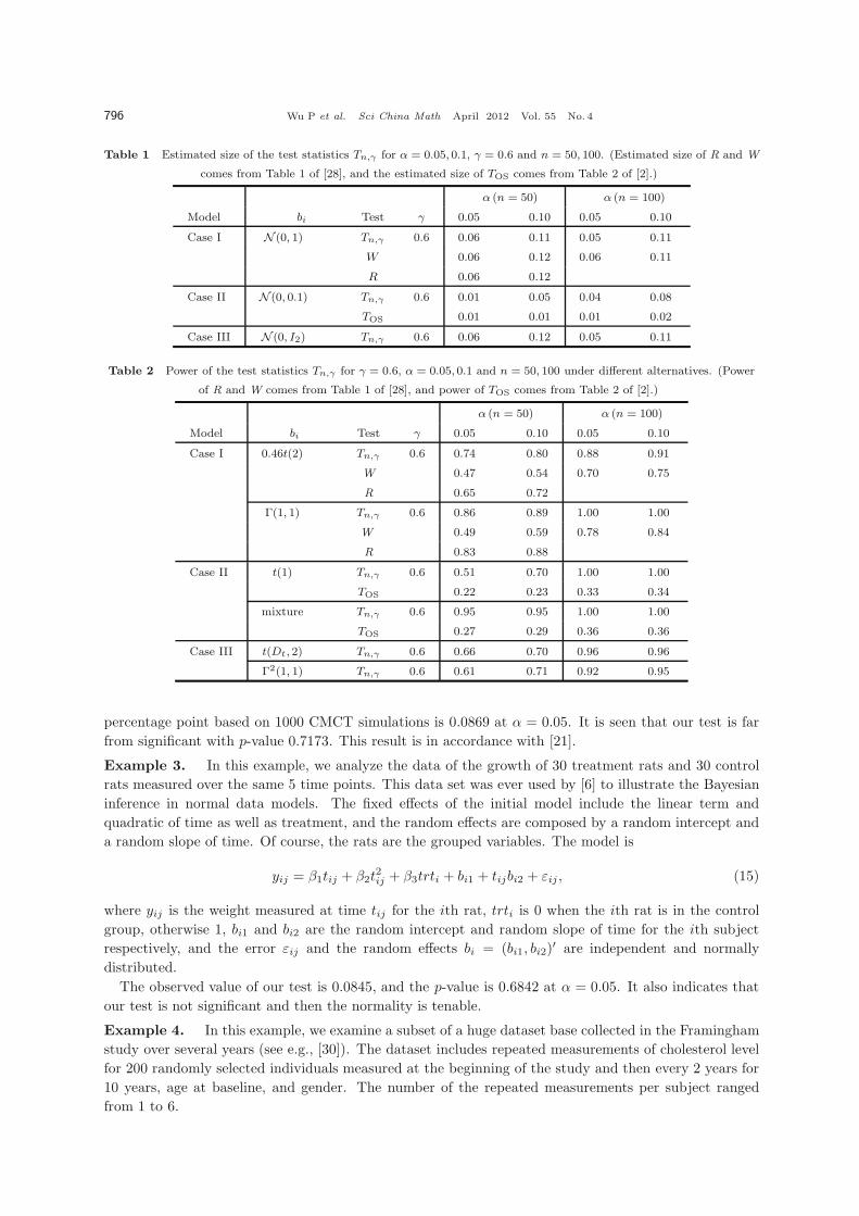
size in Table 1 under normality, and the power under different alternatives in Table 2 for γ = 0.6. To make

a comparison with R, W , TOS that were suggested by [2, 21, 28], we have cited part of their simulation

results in Table 1 [28] and Table 2 [2].

From Table 1, we can see that our test can in most cases maintain the significance level. For the

power, Table 2 shows that Tn,γ outperforms R, W and TOS in all of the cases. In conclusion, the limited

simulations suggest that the new test with γ = 0.6 is recommendable.

5.2 Applications

In this section, we apply our test to four data sets to illustrate further. From the simulation studies, the


0 2 4 6 8 10 12 14 16 18 200

102030405060708090

100110

Power (n = 50)

2 4 6 8 10 12 14 16 18 200

102030405060708090

100110

Power (n = 50)

0

α = 0.10α = 0.05

α = 0.10α = 0.05

γ γ

Pow

er

Pow

er

Figure 4 Power of the test statistics Tn,γ versus γ for bi ∼Mixnorm and sample sizes n = 50 and n = 100.

0 1 2 3 4 5 6 7 8 9 1010

20

30

40

50

60

70

80Power (n = 50)

0 1 2 3 4 5 6 7 8 9 1030

40

50

60

70

80

90

100Power (n = 100)

α = 0.10α = 0.05

α = 0.10α = 0.05

Pow

er

Pow

er

γ γ

Figure 5 Power of the test statistics Tn,γ versus γ for bi ∼ t(Dt, 2) and sample sizes n = 50 and n = 100.

0 1 2 3 4 5 6 7 8 9 1010

20

30

40

50

60

70

80Power (n = 50)

0 1 2 3 4 5 6 7 8 9 1020

30

40

50

60

70

80

90

100 Power (n = 100)

α = 0.10α = 0.05

α = 0.10α = 0.05

Pow

er

Pow

er

γ γ

Figure 6 Power of the test statistics Tn,γ versus γ for bi ∼ Γ2(1, 1) and sample sizes n = 50 and n = 100.

weight parameter is chosen to be γ = 0.6.

Example 1. We first apply our test to the data from an experiment investigating the enzyme activity

in rye bread dough. In this dataset, there are 602 observations and n = 56 groups of size 8− 12. See [4].

The observed value of our goodness-of-fit test statistics is 0.1117, and the estimated percentage point

based on 1000 CMCT simulations is 0.087 at α = 0.05. Our test is significant with a p-value of 0.018.

Ritz’s test is also highly significant (p < 0.005) but Waagepetersen’s is not (p = 0.3).

Example 2. We now consider the data set used in Example 2 of [21]. That is a part of a larger growth

study measuring the weight of chickens. There are 2017 observations and n = 169 groups of size 4− 44.

See [21] for details. The observed value of our goodness-of-fit test statistic is 0.0094, and the estimated


Table 1 Estimated size of the test statistics Tn,γ for α = 0.05, 0.1, γ = 0.6 and n = 50, 100. (Estimated size of R and W

comes from Table 1 of [28], and the estimated size of TOS comes from Table 2 of [2].)

α (n = 50) α (n = 100)

Model bi Test γ 0.05 0.10 0.05 0.10

Case I N (0, 1) Tn,γ 0.6 0.06 0.11 0.05 0.11

W 0.06 0.12 0.06 0.11

R 0.06 0.12

Case II N (0, 0.1) Tn,γ 0.6 0.01 0.05 0.04 0.08

TOS 0.01 0.01 0.01 0.02

Case III N (0, I2) Tn,γ 0.6 0.06 0.12 0.05 0.11

Table 2 Power of the test statistics Tn,γ for γ = 0.6, α = 0.05, 0.1 and n = 50, 100 under different alternatives. (Power

of R and W comes from Table 1 of [28], and power of TOS comes from Table 2 of [2].)

α (n = 50) α (n = 100)

Model bi Test γ 0.05 0.10 0.05 0.10

Case I 0.46t(2) Tn,γ 0.6 0.74 0.80 0.88 0.91

W 0.47 0.54 0.70 0.75

R 0.65 0.72

Γ(1, 1) Tn,γ 0.6 0.86 0.89 1.00 1.00

W 0.49 0.59 0.78 0.84

R 0.83 0.88

Case II t(1) Tn,γ 0.6 0.51 0.70 1.00 1.00

TOS 0.22 0.23 0.33 0.34

mixture Tn,γ 0.6 0.95 0.95 1.00 1.00

TOS 0.27 0.29 0.36 0.36

Case III t(Dt, 2) Tn,γ 0.6 0.66 0.70 0.96 0.96

Γ2(1, 1) Tn,γ 0.6 0.61 0.71 0.92 0.95

percentage point based on 1000 CMCT simulations is 0.0869 at α = 0.05. It is seen that our test is far

from significant with p-value 0.7173. This result is in accordance with [21].

Example 3. In this example, we analyze the data of the growth of 30 treatment rats and 30 control

rats measured over the same 5 time points. This data set was ever used by [6] to illustrate the Bayesian

inference in normal data models. The fixed effects of the initial model include the linear term and

quadratic of time as well as treatment, and the random effects are composed by a random intercept and

a random slope of time. Of course, the rats are the grouped variables. The model is

yij = β1tij + β2t2ij + β3trti + bi1 + tijbi2 + εij , (15)

where yij is the weight measured at time tij for the ith rat, trti is 0 when the ith rat is in the control

group, otherwise 1, bi1 and bi2 are the random intercept and random slope of time for the ith subject

respectively, and the error εij and the random effects bi = (bi1, bi2)′ are independent and normally

distributed.

The observed value of our test is 0.0845, and the p-value is 0.6842 at α = 0.05. It also indicates that

our test is not significant and then the normality is tenable.

Example 4. In this example, we examine a subset of a huge dataset base collected in the Framingham

study over several years (see e.g., [30]). The dataset includes repeated measurements of cholesterol level

for 200 randomly selected individuals measured at the beginning of the study and then every 2 years for

10 years, age at baseline, and gender. The number of the repeated measurements per subject ranged

from 1 to 6.


[30] fitted this dataset by a linear mixed model with the semi-non-parametric representation to approxi-

mating the random effects density in order to relax the normality assumption. [2] formulated a linear

mixed model and rejected the bivariate normality assumption for random effects based on OS tests.

[28] considered a linear mixed model with individual specific random intercepts and time as explanatory

variables and rejected the normality. In this one-level case, our test statistic Tn,γ has the observed value

0.3857, and the estimated percentage point based on 1000 CMCT simulations is 0.0803 at the level 0.05.

Thus our test is also highly significant because the p-value nears zero.

To check how the rate in cholesterol over time changes depends on sex and baseline age, another linear

mixed model is considered by [30] as follows. Let yij be the cholesterol level divided by 100 at the jth

time for subject i and tij is (time − 5)/10, with the time measured in years from the baseline, where

the transformations of level and time were adopted for reasons of numerical stability; agei is the age

at baseline; sexi is a gender indicator (0 = female and 1 = male). In addition, let sexi ∗ tij be the

interaction between sex and the jth measured time for the ith subject, and agei ∗ tij is similarly defined.

The linear-mixed model for yij , tij , sexi and agei with a random intercept and a random slope of time

tij is

yij = β0 + β1tij + β3sexi ∗ tij + β4agei ∗ tij + bi1 + tijbi2 + εij , (16)

where εij is within-subject error and independent of the random effect bi = (bi1, bi2)′. For γ = 0.6,

our test statistic Tn,γ has the observed value 0.5515, and the estimated percentage point based on 1000

CMCT simulations is 0.1563 at the level 0.05. Thus our test strongly suggests a rejection for normality

because the p-value nears zero. This result is also identical to [30].

6 Discussion

In this paper, we construct a BHEP test statistic (9) for any dimensional random effect in linear mixed

models. From the power study, we can see that the BHEP test works well. Furthermore, it is well known

that the finite sample behavior of the BHEP goodness-of-fit test depends on the choice of the parameter γ.

From the results of the simulations in Section 5, we recommend a working value of γ = 0.6. However

the role played by the parameter γ in the detection of departures from the null hypothesis of normality

is not very clear and needs further study. Secondly, it is seems a bit restrictive that the proposed test is

based on the assumption that the error distribution is known to be normal. In fact, before checking the

normality of the random effects, it is easy to extent our method to check that of the errors. By following

the idea of restricted maximum likelihood (see [10]), one can write the linear mixed model (1) in a matrix

form as

Y = Xβ + Zb+ ε = Wξ + ε, (17)

where Y = (Yi)1�i�n, X = (Xi)1�i�n, Zi = diag (Zi, 1 � i � n), b = (bi)1 � i � n, ε = (εi)1 � i � n,

W = (X,Z), ξ = (β′, b′)′. Let A be an N × (N − r) matrix of full rank, where N =∑n

i=1 li and

r = rank(W) (assuming r < N , which is usually the case), such that A′W = 0. For example, one can use

the QR decomposition of W to give A. Let u = A′ε, which is normal if and only if ε is normal. Then one

can use u to check the normality of ε by applying some conventional methods such as Q-Q plot, p-p plot,

and Shapiro-Wilk test. Of course, the developed method above can be applied too. The simultaneous

test for the random effects and errors also deserves further study. On the other hand, we can combine

the advantages of our test and the OS tests. That is, when the null hypothesis is rejected, we can use

the series expansions to the density functions of random effects and an order selection criterion such as

the modified AIC in [2] to provide an estimation of the random effects density. In addition, the method

is limited to testing for normality. This is because of the property of the BHEP test. It needs further

study how to construct a new testing statistic to check arbitrary distributional assumptions.

Acknowledgements The research is supported in part by a grant of Research Grants Council of Hong Kong,

and National Natural Science Foundation of China (Grant No. 11101157). The authors thank Christian Ritz for

assistance with data.


References

1 Baringhausl L, Henze N. A consistent test for multivariate normality hosed on the empirical characteristic function.

Metrika, 1988, 35: 339–348

2 Claeskens G, Hart J D. Goodness-of-fit tests in mixed models. Test, 2009, 18: 213–239

3 Claeskens G, Hart J D. Rejoinder on: goodness-of-fit tests in mixed models. Test, 2009, 18: 265–270

4 Damstrup M L, Nielsen M M. Fytaseaktivitet under rugbrøsfremstilling. Course Report, Royal Veterinary and Agri-

cultural University, Copenhagen, 2002

5 Epps T W, Pulley L B. A test for normality based on the empirical characteristic function. Biometrika, 1983, 70:

723–726

6 Gelfand A E, Hills S E, Racine-Poon A, et al. Illustration of Bayesian inference in normal data models using Gibbs

sampling. J Amer Statist Assoc, 1990, 85: 972–985

7 Harville D A. Extension of the Gauss-Markov theorem to include the estimation of random effects. Ann Statist, 1976,

4: 384–395

8 Harville D A. Maximum likelihood approaches to variance component estimation and to related problems. J Amer

Statist Assoc, 1977, 72: 320–340

9 Henze N, Wagner T. A new approach to the BHEP tests for multivariate normality. J Multivariate Anal, 1997, 62:

1–23

10 Jiang J. REML estimation: asymptotic behavior and related topics. Ann Statist, 1996, 24: 255–286

11 Jiang J. Goodness-of-fit tests for mixed model diagnostics. Ann Statist, 2001, 29: 1137–1164

12 Jiang J, Nguyen T. Comments on: goodness-of-fit tests for mixed model diagnostics. Test, 2009, 18: 248–255

13 Karatzas I, Shreve S. Brownian motion and stochastic calculus. New York: Springer-Verlag, 1991

14 Laird N M, Ware J H. Random-effects models for longitudinal data. Biometrics, 1982, 38: 963–974

15 Lang N, Ryan L. Assessing normality in random effects models. Ann Statist, 1989, 17: 624–642

16 Litiere S, Alonso A, Molenberghs G. Type I and type II error random-effects misspecification in generalized linear

mixed models. Biometrics, 2007, 63: 1038–1044

17 Litiere S, Alonso A, Molenberghs G. The impact of a misspecified random-effects distribution on the estimation and

the performance of inferential procedures in generalized linear mixed models. Stat Med, 2008, 27: 3125–3144

18 Miller J J. Asymptotic properties of maximum likelihood estimates in the mixed model of the analysis of variance.

Ann Statist, 1977, 5: 746–762

19 Molina I. Comments on: goodness-of-fit tests in mixed models. Test, 2009, 18: 244–247

20 Pierce D A. The asymptotic effect of substituting estimators for parameters in certain types of statistics. Ann Statist,

1982, 10: 545–478

21 Ritz C. Goodness-of-fit tests for mixed models. Scand J Stat, 2004, 31: 443–458

22 Tsonaka R, Verbeke G, Lesaffre E. A semi-parametric shared parameter model to handle nonmonotone nonignorable

missingness. Biometrics, 2009, 65: 81–87

23 Van der Vaart A W, Wellner J A. Weak convergence and empirical processes. New York: Springer, 1996

24 Verbeke G, Lesaffre E. Large sample properties of the maximum likelihood estimators in linear mixed models with

misspecified random-effects distributions. Technical Report, Report #1996.1 Biostatistical Centre for Clinical Trials,

Catholic University of Leuven, Belgium, 1994

25 Verbeke G, Lesaffre E. A linear mixed-effects model with heterogeneity in the random-effects population. J Amer

Statist Assoc, 1996, 91: 217–221

26 Verbeke G, Lesaffre E. The effect of misspecifying the random-effects distribution in linear mixed models for longitudinal

data. Comput Stat Data Anal, 1997, 23: 541–556

27 Verbeke G, Molenberghs G. The gradient function for checking goodness-of-fit of the random-effects distribution in

mixed models. Technical Report, Joint Statistical Meetings, Washington DC, USA, 2009

28 Waagepetersen R. A simulation-based goodness-of-fit test for random effects in generalized linear mixed models. Scand

J Stat, 2006, 33: 721–731

29 Witting H, Muller-Funk U. Mathematische Statistik II. Stuttgart: Teubner, 1995

30 Zhang D, Davidian M. Linear mixed models with flexible distributions of random effects for longitudinal data. Bio-

metrics, 2001, 57: 795–802

Appendix

Proof of Theorem 3.1. Note that

n1/2Gn(t) =1√n

n∑

i=1

[cos(t′Uni) + sin(t′Uni)− exp

{− ‖t‖2

2

}]


=1√n

n∑

i=1

[cos(t′Uni) + sin(t′Uni)− Eθ0(cos(t′uni) + sin(t′uni))]

+1√n

n∑

i=1

[Eθ0(cos(t

′uni) + sin(t′uni))− exp

{− ‖t‖2

2

}]

= n1/2G1n(t) + n1/2G2n(t), t ∈ Rq,

where the symbol Eθ0 denotes the expectation under the true parameter θ0. Then we will show that

there exists a(t; θ0) such that

n1/2G1n(t) = n1/2Gn0(t) + op(1), (A1)

and

n1/2G2n(t) = a′(t; θ0)n1/2(θ − θ0) + op(1). (A2)

Let us study (A1) first. Because of the consistency of θ, we have uni = ui(θ) = u0i+Op(n−1/2), unn =

u0n+Op(n−1/2), and then Snn = S0n+Op(n

−1). Following [9], it is easy to derive n1/2(S−10n −Iq) = Op(1)

and n1/2(S−1/20n − Iq) = Op(1). We thus obtain that S

−1/2nn = S

−1/20n +Op(n

−1). Further, we also have

uni = u0i +∂ui(θ0)

∂θ′(θ − θ0) + op(n

−1/2)

and then

Uni = S−1/2nn (uni − unn)

= S−1/20n

[u0i − u0n +

{∂ui(θ0)

∂θ′− 1

n

n∑

i=1

∂ui(θ0)

∂θ′

}(θ − θ0)

]+Op(n

−1)

= u0i +Δ0i +∂ui(θ0)

∂θ′(θ − θ0) + Δni +Op(n

−1)

with

Δ0i = (S−1/20n − Iq)u0i − S

−1/20n u0i,

and

Δni = (S−1/20n − Iq)

∂ui(θ0)

∂θ′(θ − θ0)− S

−1/20n

1

n

n∑

i=1

∂ui(θ0)

∂θ′(θ − θ0).

Let

G0n(t) =1

n

n∑

i=1

[cos(t′u0i) + sin(t′u0i)− exp

{− ‖t‖2

2

}+ {cos(t′u0i)− sin(t′u0i)}t′Δ0i

].

Following [9], we can derive that

cos(t′U0i) = cos(t′u0i)− t′Δ0i sin(t′u0i) + ζi,

sin(t′U0i) = sin(t′u0i) + t′Δ0i cos(t′u0i) + ηi,

and then ρ(n1/2(G0n(·)− G0n(·))) converges to zero in distribution, where |ζi|, |ηi| � ‖t‖2‖Δ0i‖2. Usingtrigonometric formulae, we have

cos(t′uni) = cos(t′u0i)− t′∂ui(θ0)

∂θ′(θ − θ0) sin(t

′u0i) + op(n−1/2),

sin(t′uni) = sin(t′u0i) + t′∂ui(θ0)

∂θ′(θ − θ0) cos(t

′u0i) + op(n−1/2),


cos(t′Uni) = cos(t′u0i)− t′[Δ0i +Δni +

∂ui(θ0)

∂θ′(θ − θ0) +Op

(1

n

)]sin(t′u0i) + ζni,

sin(t′Uni) = sin(t′u0i) + t′[Δ0i +Δni +

∂ui(θ0)

∂θ′(θ − θ0) +Op

(1

n

)]cos(t′u0i) + ηni,

where |ζni|, |ηni| � ‖t‖2[‖Δ0i‖2 + ‖Δni‖2 + ‖∂ui(θ0)∂θ′ (θ − θ0)‖2 + Op(n

−2)]. Recalling the definition (7)

of ui,

1

n

n∑

i=1

[∂ui(θ0)

∂θ′(cos(t′u0i)− sin(t′u0i))− Eθ0

(∂ui(θ0)

∂θ′(cos(t′u0i)− sin(t′u0i))

)]

is a sum of i.i.d. random variables and converges to zero in probability for fixed t ∈ Rq. Thus we obtain

n1/2(G1n(t)−G0n(t)) = n1/2(G1n(t)− G0n(t)) + op(1)

=1√n

n∑

i=1

[t′{Δni +Op(n−1)}(cos(t′u0i)− sin(t′u0i))]

+1√n

n∑

i=1

[ζni + ηni + ζi + ηi] + t′OP (n−1/2) + op(1). (A3)

It follows that

max‖t‖�k

n1/2|Gn1(t)− Gn0(t)| � 2k2√n

n∑

i=1

‖Δ0i‖2 + 3k2√n

n∑

i=1

‖Δni‖2

+2k2√n

n∑

i=1

∥∥∥∥∂ui(θ0)

∂θ′(θ − θ0)

∥∥∥∥2

+ op(1)

= J1 + J2 + J3 + op(1). (A4)

A similar argument to that of [9] suggests that J1 is asymptotically negligible. That is,

J1 = op(1). (A5)

A simple calculation shows that

‖Δni‖2 = (θ − θ0)′(∂ui(θ0)

∂θ′

)′(S

−1/20n − Iq)

2 ∂ui(θ0)

∂θ′(θ − θ0)

− 2(θ − θ0)′(∂ui(θ0)

∂θ′

)′(S

−1/20n − Iq)S

−1/20n

(1

n

n∑

i=1

∂ui(θ0)

∂θ′

)(θ − θ0)

+ (θ − θ0)′(1

n

n∑

i=1

∂ui(θ0)

∂θ′

)′S−10n

(1

n

n∑

i=1

∂ui(θ0)

∂θ′

)(θ − θ0),

and then

1√n

n∑

i=1

‖Δni‖2 =√ntr

(1

n

n∑

i=1

[(∂ui(θ0)

∂θ′

)′(S

−1/20n − Iq)

2 ∂ui(θ0)

∂θ′

](θ − θ0)(θ − θ0)

′)

− 2tr

((1

n

n∑

i=1

∂ui(θ0)

∂θ′

)′√n(S

−1/20n − Iq)S

−1/20n

(1

n

n∑

i=1

∂ui(θ0)

∂θ′

)(θ − θ0)(θ − θ0)

′)

+√ntr

((1

n

n∑

i=1

∂ui(θ0)

∂θ′

)′S−10n

(1

n

n∑

i=1

∂ui(θ0)

∂θ′

)(θ − θ0)(θ − θ0)

′)

= Op(n−3/2)tr

(1

n

n∑

i=1

[(∂ui(θ0)

∂θ′

)′∂ui(θ0)

∂θ′

])

− [2Op(n−1) +Op(n

−1/2)]tr

((1

n

n∑

i=1

∂ui(θ0)

∂θ′

)′1

n

n∑

i=1

∂ui(θ0)

∂θ′

)


= op(1).

The last equation holds because, by the definitions of the uis,

tr

(1

n

n∑

i=1

(∂ui(θ0)

∂θ′

)′∂ui(θ0)

∂θ′

)= Op(1), tr

((1

n

n∑

i=1

∂ui(θ0)

∂θ′

)′1

n

n∑

i=1

∂ui(θ0)

∂θ′

)= Op(1).

Thus we have

J2 = op(1). (A6)

Similarly we can derive that

J3 = op(1). (A7)

In view of (A3)–(A7) and the definition of the metric ρ(·), (A1) follows.Deal with (A2). Let ei = W

−1/2i DZ ′

iV−1i Xi(β0−β), i = 1, . . . , n. By some basic calculations, we have

Eθ(cos(t′ui) + sin(t′ui)) = exp

{− 1

2t′W−1/2

i DZ ′iV

−1i Vi0V

−1i ZiDW

−1/2i t

}(cos(t′ei) + sin(t′ei))

=: f(t;α)[cos(t′ei) + sin(t′ei)],

and, thus evaluating at θ = θ0, we have

∂Eθ0(cos(t′ui00) + sin(t′ui0))

∂θ=

(∂f(t;α0)

∂α′ ,− exp

{− ‖t‖2

2

}t′W−1/2

i0 D0Z′iV

−1i0 Xi

)′= ai(t, θ0)

′.

Using Taylor expansion, it is easy to derive

n1/2Gn2(t) =1

n

n∑

i=1

a′i(t; θ0)n1/2(θ − θ0) + op(1).

Now we calculate ∂f(t;α0)∂α′ . Recalling the definitions of Wi and Vi, we have

∂V −1i

∂σ2= −V −2

i ,∂V −1

i

∂δj= −V −1

i Zi∂D

∂δjZ ′iV

−1i ,

∂Wi

∂σ2= −DZ ′

iV−2i ZiD,

∂Wi

∂δj= DZ ′

i

∂V −1i

∂δjZiD +

∂D

∂δjZ ′iV

−1i ZiD +DZ ′

iV−1i Zi

∂D

∂δj,

vec

(∂W

1/2i

∂σ2

)= (W

1/2i ⊗ Iq + Iq ⊗W

1/2i )−1vec

(∂Wi

∂σ2

),

and

vec

(∂W

1/2i

∂δj

)= (W

1/2i ⊗ Iq + Iq ⊗W

1/2i )−1vec

(∂Wi

∂δj

).

Thus

∂f(t;α0)

∂σ2= exp(−

12 t

′t)[vec′(W−1/2

i0 tt′)vec(∂W

1/2i0

∂σ2

)+ t′W−1/2

i0 D0Z′iV

−2i0 ZiD0W

−1/2i0 t

],

∂f(t;α0)

∂δj= exp(−

12 t

′t)[vec′(W−1/2

i0 tt′)vec(∂W

1/2i0

∂δj

)− t′W−1/2

i0

∂D0

∂δjD−1

0 W−1/2i0 t

+ t′W−1/2i0 D0Z

′i

∂V −1i0

∂δjZiD0W

−1/2i0 t

].

Let

a(t, θ0) = limn→∞

1

n

n∑

i=1

ai(t; θ0). (A8)


Hence, (A2) holds. Let

G∗0n(t) =

1

n

n∑

i=1

[cos(t′u0i) + sin(t′u0i)− exp

{− ‖t‖2

2

}

+

{1

2(t′u0i)

2 − ‖t‖22

− t′u0i

}exp

{− ‖t‖2

2

}]. (A9)

Similar to [9], ρ(n1/2(G0n(·) − G∗0n(·))) converges to zero in distribution, and G∗

0n(·) is asymptotically

tight and converges in distribution to G0(·) in C(Rq) with covariance (kernel) function (10). Thus the

process Gn(·) can be written as

√nGn(t) =

√nG∗

0n(t) + a′(t; θ0)√n(θ − θ0) + op(1), (A10)

and is also asymptotically tight.

To derive the limiting process of√nGn(t), combining the asymptotic tightness of the process, Theorem

1.5.4 of [23] implies that what we need to do now is to show the convergence of the following marginal,

for any finite set of points t1, . . . , tm ∈ Rq,

n1/2(G∗0n(t1), . . . , G

∗0n(tm), (θ − θ0)

′, . . . , (θ − θ0)′

︸︷︷︸)′

to normal variables.

Assume that, recalling Qi of (5), Eθ0Qi(yi, θ0) = 0, Eθ0‖Qi(yi, θ0)‖2 < ∞ and Eθ0‖Qi(yi, θ0)‖3 < ∞.

It is seen that∑n

i=1 E‖Qi(yi; θ0)‖3 is O(n) and thus must be o(n3/2) as n tends to infinity. For any

constants c1 ∈ Rp+k+1, c2 ∈ R and t1, . . . , tm ∈ Rq with a fixed integer m,∑n

i=1 Eθ0 |c′1Qi(Yi; θ0) + c2Q∗i |3

(∑n

i=1 Eθ0 |c′1Qi(Yi; θ0) + c2Q∗i |2)3/2

should tend to 0 as n tends to ∞. Here

Q∗i =

m∑

j=1

[cos(t′ju0i) + sin(t′ju0i)− exp

{− ‖tj‖2

2

}+

{1

2(t′ju0i)

2 − ‖tj‖22

− t′ju0i

}exp

{− ‖tj‖2

2

}].

In fact, E|Q∗i |3 is a constant that depends on m, (ti)1�i�m, and

n∑

i=1

Eθ0 |c′1Qi(Yi; θ0) + c2Q∗i |2 = O(n).

Then∑n

i=1 E‖Qi(yi; θ0)‖3 = o(n3/2) implies that the above ratio tends to 0. By the Cramer-Wold device

and Lyapunov condition of central limit theorems (CLT), we have that

n1/2(G∗0n(t1), . . . , G

∗0n(tm), (θ − θ0)

′, . . . , (θ − θ0)′

︸︷︷︸)′

converges in distribution to

N(0,

(Σ11 Σ12

Σ21 Σ22

)),

with Σ11 = (K0(ti, tj))1�i,j�m, Σ22 = Im ⊗ Ω−1, and Σ12 = Σ′21 the correlation matrix. It follows from

[20] that n1/2(Gn(t1), . . . , Gn(tm))′ converges in distribution to

N (0,Σ11 − [a′(t1, θ0), . . . , a′(tm, θ0)]′Σ22[a

′(t1, θ0), . . . , a′(tm, θ0)]).

Then the marginals of Gn(t) converge in distribution to a multivariate normal distribution.

By Theorem 1.5.4 in [23], the asymptotic tightness and asymptotic normality in the previous proof

imply that Gn(t) converges in distribution to a tight Gaussian process in C(Rq) having zero mean and

covariance (kernel) function defined in (11).


Proof of Corollary 3.1. Based on the proof of Theorem 3.1, we have

Gn(t) = G0n(t) + a′(t; θ0)n1/2(θ − θ0) + op(1)

= G0n(t) + a′(t; θ0)n1/2(θ − θ0) + op(1)

= G∗0n(t) + a′(t; θ0)n1/2(θ − θ0) + op(1)

and ∫

t∈Rq

a(t)′Ω−1a(t)ϕγ(t)dt � ∞.

Thus the proof of this corollary is essentially the same as that of Theorem 2.2 of [9]. Readers can refer

to it for details.

Proof of Theorem 3.2. We consider α = 1/2 first. When α < 1/2, we can easily derive the result from

the argument used below.

Based on (5) and (A10), the counterpart of Gn under the triangular array {(Yni, Xni, Zni, lni)}ni=1 is

Gnn(t) =1

n

n∑

i=1

[cos(t′uni(θ0)) + sin(t′uni(θ0))− exp

{− ‖t‖2

2

}

+

{1

2(t′uni(θ0))

2 − ‖t‖22

− t′uni(θ0)

}exp

{− ‖t‖2

2

}]

+ a′(t; θ0)Ω−10

1

n

n∑

i=1

Qni(Yni −Xniβ0; θ0) + op(n−1/2)

= G∗nn(t) + op(n

−1/2). (A11)

Recalling uni(θ0) = W−1/20i D0Z

′niV

−10i (Yni −Xniβ0), we have

Yni −Xniβ0 = (Ini − σ20V

−10i )−1ZniW

1/20i uni(θ0).

Hence G∗nn(t) is stochastic up to uni(θ0). On the other hand, under the alternatives of (12), it is not

difficult to derive the corresponding density functions of the uni(θ0)s,

fni(u; θ0) = ϕq(u)(1 + n−1/2hni(u; θ0)), (A12)

where ϕq(·) is a standard q-dimensional normal density, and

hni(u; θ0) = (2π)−q2 |Σi|− 1

2

∫

x∈Rq

exp

{− 1

2(x−W

−1/2i u)′Σ−1

i (x−W−1/2i u)

}h(x)dx,

where Σi = D−1 − W−1i . Moreover,

∫u∈Rq hni(u; θ)ϕq(u)du = 0. Then we just need to derive the

asymptotic behavior ofG∗nn(t) under the new alternative density functions (A12) of the responses uni(θ0)s.

Following [9], we consider the probability measures

P (n) =n⊗

i=1

(ϕ(·)λq) and Q(n) =n⊗

i=1

(fni(·; θ0)λq)

on the measurable space (Xn,Bn) =⊗n

i=1(Rq,Bq), where λq is Lebesgue measure on the Borel sets Bq

of Rq. Putting Ln := dQ(n)/dP (n), we have

logLn(un1(θ0), . . . , unn(θ0)) =n∑

i=1

log(1 + n−1/2hni(uni(θ0); θ0))

=

n∑

i=1

(n−1/2hni(uni(θ0); θ0)− h2

ni(uni(θ0); θ0)

2n

)+ oP (n)(1).


Some elementary calculations yield

E logLn = − 1

2n

n∑

i=1

σ2i and Var (logLn) =

1

n

n∑

i=1

σ2i ,

where σ2i =

∫u∈Rq h

2ni(u; θ0)ϕq(u)dy < ∞. Let ζni =

hni(uni(θ0);θ0)

n1/2 −h2ni(uni(θ0);θ0)

2n +σ2i

2n and B2n = Var(Ln).

It is easy to see that∑n

i=1 Eζ3ni = oP (n)(1). By the Lyapunov’s central limit theorem and weak law of

large numbers (WLLN), logLn converges to N (−σ2

2 , σ2) under P (n), where σ2 = limn→∞ B2n. Under

P (n), we have

C(t) = limn→∞Cov(

√nG∗

0nn(t), logLn)

= limn→∞

1

n

n∑

i=1

∫

u∈Rq

(g(u, t) + a′(t; θ0)Ω−10 Qni(u; θ0))hni(u; θ0)ϕq(u)du, (A13)

where

g(u, t) = cos(t′u) + sin(t′u)− exp

{− ‖t‖2

2

}+

{1

2(t′u)2 − 1

2‖t‖2 − t′u

}exp

{− ‖t‖2

2

}.

For any fixed m ∈ R and t1, . . . , tm ∈ Rq, similar to the proof of Theorem 3.1, we can show that the

joint limiting distribution of

n1/2

(G∗

nn(t1), . . . , G∗nn(tm), logLn − σ2

2

)′

is a zero mean normal random vector with covariance matrix(

Σ C

C′ σ2

),

where Σ = (K(ti, tj))1�i,j�m and C = (C(t1), . . . , C(tm))′. By Le Cam’s lemma, the sequence Q(n) is

contiguous to P (n). Please see [29, p. 311]. Invoking Le Cam’s third lemma (see, e.g., [29, p. 329]), we thus

obtain that, under Q(n), the finite dimensional distributions of G∗nn(t) converge to the finite dimensional

distributions of the shifted Gaussian process G(t) + C(t). Since tightness of G∗nn(t) under P

(n) and the

contiguity of Q(n) to P (n) imply tightness of G∗nn(t) under Q

(n), the assertion of Theorem 3.2 follows.

Proof of Theorem 4.1. Under the local alternatives of (12), results in [10] show that the MLE is still con-

sistent. For almost all sequences {(Xi, Zi, li, Yi)}, it follows that the covariance function of√nGn(Y0n, t)

has the same limit as√nGn(t), and by CLT, the finite-dimensional convergence of

√nGn(Y0n, t) also

holds. According to Theorem 1.5.4 in [23], what remains to show for process convergence is asymptotic

tightness. Adapting the arguments used in [13] to the present case, all we need to do is to show that for

each k � 1 the sequence√nGn(Y0n, t), restricted to Rq

k = {t ∈ Rq : ‖t‖ � k}, is asymptotically tight in

the Banach space C(Rqk). From the consistency of θ again, one can obtain

√nGn(Y0n, t) =

1√n

n∑

i=1

[cos(t′u0i(Y0i)) + sin(t′u0i(Y0i))− exp

{− ‖t‖2

2

}

+

{1

2(t′u0i(Y0i))

2 − ‖t‖22

− t′u0i(Y0i)

}exp

{− ‖t‖2

2

}]

+ a′(t; θ0)Ω−10

1√n

n∑

i=1

Qi(Y0i; θ0) + op(1).

Assume that there exists some constant c such that ‖a(s; θ0) − a(t; θ0)‖ � c‖s − t‖. By the proof of

Theorem 2.1 of [9], thus, the property of asymptotic tightness of√nGn(Y0n, t) follows. By Corollary 3.1,

we complete the proof.

Date post:	26-Aug-2016
Category:	Documents
Upload:	ping-wu
View:	213 times
Download:	1 times

Checking for normality in linear mixed models

Documents