179
| Date post: | 27-Oct-2015 |
| Category: |
Documents |
| Upload: | iqcesar1651 |
| View: | 561 times |
| Download: | 43 times |

THE CHEMSEP BOOK
TECHNICAL DOCUMENTATION
Copyright (c), H.A. Kooijman, R. Taylor
October 1998
iii
Preface
This book accompanies the ChemSep program, which was developed to allow students to
do separation calculations on ordinary personal computers. This book is not a guide where
we show how to use ChemSep (see the ChemSep user manual for that) but it is intended
to supply technical background to help the user in his selection of models and correlations.
It is hoped that sensible selections can be made by providing information on, descriptions of,
and references to the models and correlations that are employed in ChemSep. Although
we have tried to be as extensive as possible, it is impossible to describe all models and
their underlaying theory, so references are given for further reading. There are probably
many more literature models and correlations than are available in ChemSep, but we
have tried to be as comprehensive as we could. Sometimes a choice had to be made in
which models to implement without having any criteria to discriminate between models.
Furthermore, not all models are applicable to a particular regime of operation. We try
to adapt ChemSep as much as possible to comply with all model limitations and user
requirements. This book serves as a replacement for the \manual" information �les that
we used to distribute with ChemSep. Therefore, some parts of this document might still
be incomplete or unorganized and any suggestions or remarks are welcome. Of course, any
remarks on the ChemSep program are welcome as well.
This book is written in LATEX, a complete typesetting language, and set in the standard
Times-Roman 11 point font. It is also provided with ChemSep in ASCII text form (�le
CHEMSEP.TXT) for online reference which was generated with a LATEX to ASCII converter.
The conversion is limited, with the result that the ASCII text �le contains some unconverted
LATEX formatting. A PostScript �le (BOOK.PS) also generated by LATEX can be downloaded
from our ftp site.
Harry Kooijman
Ross Taylor
v

Acknowledgements
Many people have helped to shape ChemSep. The project was started in 1988 at Delft
University (The Netherlands) by Harry Kooijman, Arno Haket and Ross Taylor. The
purpose was to make an interactive interface for doing equilibrium stage calculations on the
PC platform. It had to be easy enough for use by students with little computer exposure
and yet su�ciently comprehensive to solve the various problems encountered in a course on
separation processes.
We would like to express our appreciation to Professor Hans Wesselingh (now at the Uni-
versity of Groningen, the Netherlands) who initially promoted the project and made various
resources available and encouraged us by letting students use the program for their course
work. This has been an indispensable source of feedback that has helped us to improve
the program. We also like to thank Peter Verheijen for his enthusiasm and contributions in
the early years of the project. Also, various students have worked on projects to check and
improve the programs and documentation, which was very helpful. Finally, ChemSep owes
its very existence to the Internet which enabled the authors to keep in touch and continue
development while living on di�erent continents.
vi

Contents
Preface v
Acknowledgements vi
1 Solving Nonlinear Equations 1
1.1 Newton's method . . . . . . . . . . . . . . . . . . . . . . . . . . . . . . . . . 1
1.2 Continuation method . . . . . . . . . . . . . . . . . . . . . . . . . . . . . . . 3
2 Property Models 5
2.1 Thermodynamic Properties . . . . . . . . . . . . . . . . . . . . . . . . . . . 5
2.1.1 K-value models . . . . . . . . . . . . . . . . . . . . . . . . . . . . . . 5
2.1.2 Activity coe�cient models . . . . . . . . . . . . . . . . . . . . . . . . 6
2.1.3 Vapour pressure models . . . . . . . . . . . . . . . . . . . . . . . . . 9
2.1.4 Equations of State (EOS) . . . . . . . . . . . . . . . . . . . . . . . . 10
2.1.5 Virial EOS . . . . . . . . . . . . . . . . . . . . . . . . . . . . . . . . 10
2.1.6 Cubic EOS . . . . . . . . . . . . . . . . . . . . . . . . . . . . . . . . 11
2.1.7 Enthalpy . . . . . . . . . . . . . . . . . . . . . . . . . . . . . . . . . 14
2.2 Physical Properties . . . . . . . . . . . . . . . . . . . . . . . . . . . . . . . . 14
2.2.1 Liquid density . . . . . . . . . . . . . . . . . . . . . . . . . . . . . . 17
vii

2.2.2 Vapour density . . . . . . . . . . . . . . . . . . . . . . . . . . . . . . 19
2.2.3 Liquid Heat Capacity . . . . . . . . . . . . . . . . . . . . . . . . . . 20
2.2.4 Vapour Heat Capacity . . . . . . . . . . . . . . . . . . . . . . . . . . 20
2.2.5 Liquid Viscosity . . . . . . . . . . . . . . . . . . . . . . . . . . . . . 20
2.2.6 Vapour Viscosity . . . . . . . . . . . . . . . . . . . . . . . . . . . . . 22
2.2.7 Liquid Thermal Conductivity . . . . . . . . . . . . . . . . . . . . . . 25
2.2.8 Vapour Thermal Conductivity . . . . . . . . . . . . . . . . . . . . . 26
2.2.9 Liquid Di�usivity . . . . . . . . . . . . . . . . . . . . . . . . . . . . . 28
2.2.10 Vapour Di�usivity . . . . . . . . . . . . . . . . . . . . . . . . . . . . 30
2.2.11 Surface Tension . . . . . . . . . . . . . . . . . . . . . . . . . . . . . . 31
2.2.12 Liquid-Liquid Interfacial Tension . . . . . . . . . . . . . . . . . . . . 32
3 Flash Calculations 37
3.1 Equations . . . . . . . . . . . . . . . . . . . . . . . . . . . . . . . . . . . . . 37
3.2 Solution of the Flash Equations . . . . . . . . . . . . . . . . . . . . . . . . . 39
4 Equilibrium Columns 41
4.1 Introduction . . . . . . . . . . . . . . . . . . . . . . . . . . . . . . . . . . . . 41
4.2 Equations . . . . . . . . . . . . . . . . . . . . . . . . . . . . . . . . . . . . . 43
4.3 Condenser and Reboiler . . . . . . . . . . . . . . . . . . . . . . . . . . . . . 44
4.4 "Nonequilibrium" Stages . . . . . . . . . . . . . . . . . . . . . . . . . . . . . 45
4.5 Solution of the MESH Equations . . . . . . . . . . . . . . . . . . . . . . . . 46
4.5.1 How to Order the Equations and Variables? . . . . . . . . . . . . . . 46
4.5.2 The Jacobian . . . . . . . . . . . . . . . . . . . . . . . . . . . . . . . 47
4.5.3 How Should the Linearized Equations be Solved? . . . . . . . . . . . 48
viii
4.5.4 The Initial Guess . . . . . . . . . . . . . . . . . . . . . . . . . . . . . 48
4.5.5 Reliability . . . . . . . . . . . . . . . . . . . . . . . . . . . . . . . . . 50
4.5.6 Damping factors . . . . . . . . . . . . . . . . . . . . . . . . . . . . . 50
4.5.7 User Initialization . . . . . . . . . . . . . . . . . . . . . . . . . . . . 51
4.5.8 Initialization with Old Results . . . . . . . . . . . . . . . . . . . . . 51
5 Nonequilibrium Columns 55
5.1 The Nonequilibrium Model . . . . . . . . . . . . . . . . . . . . . . . . . . . 55
5.2 Mass Transfer Coe�cient Correlations . . . . . . . . . . . . . . . . . . . . . 63
5.2.1 Trays . . . . . . . . . . . . . . . . . . . . . . . . . . . . . . . . . . . 64
5.2.2 Random Packings . . . . . . . . . . . . . . . . . . . . . . . . . . . . 67
5.2.3 Structured packings . . . . . . . . . . . . . . . . . . . . . . . . . . . 69
5.3 Flow Models . . . . . . . . . . . . . . . . . . . . . . . . . . . . . . . . . . . 71
5.3.1 Mixed ow . . . . . . . . . . . . . . . . . . . . . . . . . . . . . . . . 71
5.3.2 Plug ow . . . . . . . . . . . . . . . . . . . . . . . . . . . . . . . . . 71
5.3.3 Dispersion ow . . . . . . . . . . . . . . . . . . . . . . . . . . . . . . 72
5.4 Pressure Drop Models . . . . . . . . . . . . . . . . . . . . . . . . . . . . . . 72
5.4.1 Tray pressure drop estimation . . . . . . . . . . . . . . . . . . . . . . 73
5.4.2 Random packing pressure drop correlations . . . . . . . . . . . . . . 75
5.4.3 Structured packing pressure drop correlations . . . . . . . . . . . . . 77
5.5 Entrainment and Weeping . . . . . . . . . . . . . . . . . . . . . . . . . . . . 79
5.6 The Design Mode . . . . . . . . . . . . . . . . . . . . . . . . . . . . . . . . . 79
5.6.1 Tray Design: Fraction of ooding . . . . . . . . . . . . . . . . . . . . 80
5.6.2 Packing Design: Fraction of ooding . . . . . . . . . . . . . . . . . . 84
ix

5.6.3 Pressure drop . . . . . . . . . . . . . . . . . . . . . . . . . . . . . . . 84
5.6.4 Optimizing . . . . . . . . . . . . . . . . . . . . . . . . . . . . . . . . 85
6 Nonequilibrium Extraction 91
6.1 Introduction . . . . . . . . . . . . . . . . . . . . . . . . . . . . . . . . . . . . 91
6.2 Sieve trays . . . . . . . . . . . . . . . . . . . . . . . . . . . . . . . . . . . . . 92
6.2.1 Design . . . . . . . . . . . . . . . . . . . . . . . . . . . . . . . . . . . 92
6.2.2 Report . . . . . . . . . . . . . . . . . . . . . . . . . . . . . . . . . . . 94
6.2.3 Mass Transfer Coe�cients . . . . . . . . . . . . . . . . . . . . . . . . 95
6.3 Packed columns . . . . . . . . . . . . . . . . . . . . . . . . . . . . . . . . . . 95
6.3.1 Design . . . . . . . . . . . . . . . . . . . . . . . . . . . . . . . . . . . 95
6.3.2 Report . . . . . . . . . . . . . . . . . . . . . . . . . . . . . . . . . . . 96
6.3.3 Mass Transfer Coe�cients . . . . . . . . . . . . . . . . . . . . . . . . 97
6.4 Rotating Disk Contactors . . . . . . . . . . . . . . . . . . . . . . . . . . . . 98
6.4.1 Design . . . . . . . . . . . . . . . . . . . . . . . . . . . . . . . . . . . 98
6.4.2 Report . . . . . . . . . . . . . . . . . . . . . . . . . . . . . . . . . . . 99
6.4.3 Mass Transfer Coe�cients . . . . . . . . . . . . . . . . . . . . . . . . 100
6.5 Spray columns . . . . . . . . . . . . . . . . . . . . . . . . . . . . . . . . . . 101
6.5.1 Design . . . . . . . . . . . . . . . . . . . . . . . . . . . . . . . . . . . 101
6.5.2 Report . . . . . . . . . . . . . . . . . . . . . . . . . . . . . . . . . . . 101
6.5.3 Mass Transfer Coe�cients . . . . . . . . . . . . . . . . . . . . . . . . 102
6.6 Modeling Back ow . . . . . . . . . . . . . . . . . . . . . . . . . . . . . . . . 103
7 Interface and Technical Issues 113
7.1 ChemSep Commandline Parameters . . . . . . . . . . . . . . . . . . . . . . 113
x
7.2 ChemSep Environment Variables . . . . . . . . . . . . . . . . . . . . . . . . 114
7.2.1 CauseWay DOS extender . . . . . . . . . . . . . . . . . . . . . . . . 114
7.2.2 Rational . . . . . . . . . . . . . . . . . . . . . . . . . . . . . . . . . . 115
7.2.3 SVGA drivers . . . . . . . . . . . . . . . . . . . . . . . . . . . . . . . 115
7.2.4 Printer drivers . . . . . . . . . . . . . . . . . . . . . . . . . . . . . . 115
7.3 ChemSep's Programs . . . . . . . . . . . . . . . . . . . . . . . . . . . . . . . 116
7.4 Running ChemSep - Advanced Use . . . . . . . . . . . . . . . . . . . . . . . 118
7.5 ChemSep Libraries and Other Files . . . . . . . . . . . . . . . . . . . . . . . 119
7.6 The SEP-�le format . . . . . . . . . . . . . . . . . . . . . . . . . . . . . . . 124
7.7 Printing graphs in ChemSep . . . . . . . . . . . . . . . . . . . . . . . . . . . 128
7.8 Model De�nition and Selection . . . . . . . . . . . . . . . . . . . . . . . . . 129
7.9 Author and program information . . . . . . . . . . . . . . . . . . . . . . . . 131
8 FlowSheeting 133
8.1 Flowsheet Input File . . . . . . . . . . . . . . . . . . . . . . . . . . . . . . . 133
8.2 Flowsheet execution . . . . . . . . . . . . . . . . . . . . . . . . . . . . . . . 138
8.3 Flowsheet Analysis . . . . . . . . . . . . . . . . . . . . . . . . . . . . . . . . 138
8.4 Convergence . . . . . . . . . . . . . . . . . . . . . . . . . . . . . . . . . . . . 140
8.5 Mass Balances . . . . . . . . . . . . . . . . . . . . . . . . . . . . . . . . . . 140
8.6 Stream Report . . . . . . . . . . . . . . . . . . . . . . . . . . . . . . . . . . 141
8.7 Commandline Options . . . . . . . . . . . . . . . . . . . . . . . . . . . . . . 142
8.8 Other Unit Operations . . . . . . . . . . . . . . . . . . . . . . . . . . . . . . 143
8.8.1 Simple Reactor . . . . . . . . . . . . . . . . . . . . . . . . . . . . . . 143
8.8.2 Make-Up Feeds . . . . . . . . . . . . . . . . . . . . . . . . . . . . . . 145
xi
8.8.3 Stream Splitter . . . . . . . . . . . . . . . . . . . . . . . . . . . . . . 146
8.9 Examples . . . . . . . . . . . . . . . . . . . . . . . . . . . . . . . . . . . . . 147
8.9.1 Extractive Distillation (PH) . . . . . . . . . . . . . . . . . . . . . . . 147
8.9.2 Distillation with a Heterogeneous Azeotrope (BW) . . . . . . . . . . 147
8.9.3 Distillation of a Pressure Sensitive Azeotrope (MA) . . . . . . . . . 150
8.9.4 Petyluk Columns (PETYLUK) . . . . . . . . . . . . . . . . . . . . . 150
8.9.5 Extraction with Solvent Recovery (BP) . . . . . . . . . . . . . . . . 150
9 ChemProp 155
9.1 Input . . . . . . . . . . . . . . . . . . . . . . . . . . . . . . . . . . . . . . . . 155
9.2 Results . . . . . . . . . . . . . . . . . . . . . . . . . . . . . . . . . . . . . . . 155
9.2.1 Component properties . . . . . . . . . . . . . . . . . . . . . . . . . . 155
9.2.2 Mixture properties . . . . . . . . . . . . . . . . . . . . . . . . . . . . 156
9.2.3 Tables . . . . . . . . . . . . . . . . . . . . . . . . . . . . . . . . . . . 156
9.2.4 Graphs . . . . . . . . . . . . . . . . . . . . . . . . . . . . . . . . . . 156
9.2.5 Phase diagrams . . . . . . . . . . . . . . . . . . . . . . . . . . . . . . 156
9.2.6 Di�usivities . . . . . . . . . . . . . . . . . . . . . . . . . . . . . . . . 156
9.3 Various . . . . . . . . . . . . . . . . . . . . . . . . . . . . . . . . . . . . . . 157
10 ChemLib 159
10.1 Pure Component Data �les . . . . . . . . . . . . . . . . . . . . . . . . . . . 159
10.1.1 Name and library index . . . . . . . . . . . . . . . . . . . . . . . . . 160
10.1.2 Structure . . . . . . . . . . . . . . . . . . . . . . . . . . . . . . . . . 160
10.1.3 Family . . . . . . . . . . . . . . . . . . . . . . . . . . . . . . . . . . . 160
10.1.4 Critical properties and triple/melting/boiling points . . . . . . . . . 160
xii

10.1.5 Molecular parameters . . . . . . . . . . . . . . . . . . . . . . . . . . 161
10.1.6 Heats/energies/entropies . . . . . . . . . . . . . . . . . . . . . . . . . 161
10.1.7 Temperature correlations . . . . . . . . . . . . . . . . . . . . . . . . 161
10.1.8 Miscellaneous parameters . . . . . . . . . . . . . . . . . . . . . . . . 162
10.1.9 Thermodynamic model parameters . . . . . . . . . . . . . . . . . . . 162
10.1.10Group contribution methods . . . . . . . . . . . . . . . . . . . . . . 162
10.2 Making a new library . . . . . . . . . . . . . . . . . . . . . . . . . . . . . . 163
10.3 Editing a library . . . . . . . . . . . . . . . . . . . . . . . . . . . . . . . . . 163
10.3.1 Edit/View Library Label . . . . . . . . . . . . . . . . . . . . . . . . 163
10.3.2 Change/Browse Component . . . . . . . . . . . . . . . . . . . . . . . 163
10.3.3 Deleting Components . . . . . . . . . . . . . . . . . . . . . . . . . . 163
10.3.4 Moving Components . . . . . . . . . . . . . . . . . . . . . . . . . . . 163
10.3.5 Importing/New Components . . . . . . . . . . . . . . . . . . . . . . 164
10.3.6 Exporting Components . . . . . . . . . . . . . . . . . . . . . . . . . 164
10.3.7 Updating Components . . . . . . . . . . . . . . . . . . . . . . . . . . 164
10.3.8 Checking Components . . . . . . . . . . . . . . . . . . . . . . . . . . 164
10.3.9 Estimating Components . . . . . . . . . . . . . . . . . . . . . . . . . 164
10.3.10Making Pseudo Components . . . . . . . . . . . . . . . . . . . . . . 165
10.3.11 Estimating Properties for a New Component . . . . . . . . . . . . . 165
10.3.12UNIFAC methods . . . . . . . . . . . . . . . . . . . . . . . . . . . . 165
10.3.13Tb and SG methods . . . . . . . . . . . . . . . . . . . . . . . . . . . 166
10.4 Other ChemLib Files . . . . . . . . . . . . . . . . . . . . . . . . . . . . . . . 167
10.5 References . . . . . . . . . . . . . . . . . . . . . . . . . . . . . . . . . . . . . 167
xiii

Chapter 1
Solving Nonlinear Equations
In this chapter we discuss the methods employed in ChemSep to solve the separation
problems at hand. Side-issues such as how to start an iterative method or how ChemSep
solves the resulting linear system of equations also pass the revue.
1.1 Newton's method
ChemSep uses Newton's method to solve the system of (MESH) equations derived from
the ash or column problems. Newton's method is a Simultaneous Correction (SC) method
that each time corrects all the variables. To use it, the equations to be solved are written
in the form
F (x) = 0 (1.1)
where F is a vector consisting of all the equations to be solved and x is, again, the vector of
variables. A Taylor series expansion of the function vector around the point xo which the
functions are evaluated gives (ignoring second and higher order terms):
F (x) = F (xo) + J(x� xo) (1.2)
where J is the Jacobian matrix of partial derivatives of F with respect to the independent
variables x:
Jij =@Fi
@xj(1.3)
If x is the actual solution to the system of equations, then F (x) = 0 and we can rewrite the
above equation as:
J(x� xo) = �F (xo) (1.4)
This linear system of equations may be solved for a new estimate of the vector x. If the
new vector, x, obtained in this way does not actually satisfy the set of equations, F , then
1

p g q
the procedure can be repeated using the calculated x as a new x. The entire procedure is
summarized below.
1. Set iteration counter, k, to zero, estimate xo
2. Solve linearized equations for xk+1
3. Check for convergence; if not obtained, increment k and return to step 2.
Solving the linear system does not require a full matrix inversion of the Jacobian and is
normaly done with Gaussian elimination or some type of decomposition technique. If the
Jacobian has a lot of zero entries (i.e. it is sparse) then the linear system can be much more
e�ciently solved by using a sparse linear solver. For Jacobians with speci�c structures
special solvers can be employed which are more e�cient than a complete elimination or
decomposition.
One very important property of the Newton's method is that the convergence is scale
invariant and independent of the ordering of the equations. This means that the same
convergence is obtained if one of the equations is multiplied by some number or if the
equations are reordered in a di�erent manner. This is very important, because this means
we are free to order the equations to obtain a special Jacobian which might enable the use
of a special solver. It also makes the method applicable to a wider range of problems and
without requiring the user to scale equations or variables.
An important drawback of the Newton's method can be its sensitivity to the initial guess,
xo, since quadratic convergence is only achieved \close" to the solution. In order to obtain
convergence, Newton's method requires that reasonable initial estimates be provided for
all independent variables. It is obviously impractical to expect the user of a SC method
to guess this number of quantities. Thus, the designer of a computer code implementing
a SC method must provide one or more methods of generating initial estimates of all the
unknown variables. Several techniques have been developed to improve the convergence
away from the solution and to prevent the method from taking a step in a wrong direction.
The simplest and most common technique is to \damp" the step of each variable to some
range or fraction of the Newton step. However, this damping also reduces the methods
e�ectiveness.
Simultaneous correction procedures have shown themselves to be generally fast and reliable,
having a locally quadratic convergence rate in the case of Newton's method, and these meth-
ods are much less sensitive to di�culties associated with nonideal problems than are tearing
methods. They also lend themselves to be easier extended with optimization, parametric
sensitivity, or continuation methods.
1.2 Continuation method
A simple implementation of a continuation method is incorporated in ChemSep for more
di�cult problems. Continuation methods use a parameter to make a path from a known
solution for a simpli�ed model to the desired solution of the complete model. For example
the Newton homotopy starts with the initial guess as model and follows the path to the
solution of the real problem by solving
0 = (1� t)(F (Xo)� F (X)) + tF (X) (1.5)
where t varies from 0 (where X = Xo) to 1 (where F (X) = 0). Better continuation
methods can be formulated while using a parameter which has some physical signi�cance.
In separations problems the most appropriate choice would be the degree to which mass
transfer (between the present phases) prevails. In the equilibriummodel the stage e�ciency
and in the nonequilibrium model the mass transfer rates represent this degree. Thus, they
will be multiplied with a parameter t which will vary from 0 (no separation at all) to 1
(actual separation).

p g q
Chapter 2
Property Models
This chapter discusses the thermodynamic and physical property models available inChem-
Sep. The selection of these models can be quite important for the results produced by
ChemSep. Most formulae are repeated here but additional reading is available in two
main sources:
A: R.C. Reid, J.M. Prausnitz and B.E. Poling, The Properties of Gases and Liquids, 4th
Ed., McGraw-Hill, New York (1988).
B: S.M. Walas, Phase Equilibria in Chemical Engineering, Butterworth Publishers, Lon-
don (1985).
References are in between parentheses, by combining the letter A or B with the page number,
for example (A43). The model "types" are grouped by ChemSep menu.
2.1 Thermodynamic Properties
2.1.1 K-value models
Ideal (A251,B548) K-values for ideal mixtures are given by Raoult's law:
Ki =Pvap;i
P(2.1)
EOS (A319,B301) K-values are calculated from the ratio of fugacity coe�cients:
Ki =�Li
�Vi
(2.2)
5
p p y
where the fugacity coe�cients are calculated from an equation of state. This model
is recommended for separations involving mixtures of hydrocarbons and light gases
(hydrogen, carbondioxide, nitrogen, etc.) at low and high pressures. It is not recom-
mended for nonideal chemical mixtures at low pressures. The EOS must be able to
predict vapour as well as liquid fugacity coe�cients.
Gamma-Phi (A250,B301) K-Values are calculated from:
Ki = i�
�iP �iPFi
�ViP
(2.3)
This option should be used when dealing with nonideal uid mixtures. It should not
be selected for separations at high pressures.
DECHEMA (B301) K-values are calculated from a simpli�ed form of the complete Gamma-Phi
model in which the vapour phase fugacity coe�cient and Poynting correction factor
are assumed equal to unity:
Ki = iP
�i
P(2.4)
This is the form of the K-value model used in the DECHEMA compilations of equilib-
rium data (Hence the name given to this menu option). DECHEMA uses the Antoine
equation to compute the vapour pressures but ChemSep allows you to choose other
vapour pressure models if you wish. This option should be used when dealing with
non-ideal uid mixtures. It should not be selected for separations at high pressures.
Chao-Seader (B303) The Chao-Seader method is widely used for mixtures of hydrocarbons and light
gases. It is not recommended for nonideal mixtures. The method uses the Regular
solution model for the liquid phase and the Redlich Kwong EOS for the vapour phase.
An alternative choice would be the Equation of State option.
Polynomial (B11) Calculate K-value as function of the absolute temperature (Kelvin):
K1=mi
i= Ai +BiT + CiT
2 +DiT3 +EiT
4 (2.5)
You must supply the coe�cients A through E and the exponent m.
2.1.2 Activity coe�cient models
Here we discuss the activity coe�cient models available in ChemSep. For an in depth
discussion of these models see the standard references. For the calculation of activity
coe�cients and their derivatives (for di�usion calculations) see also Kooijman and Taylor
(1991).
Ideal For an ideal system the activity coe�cient of all species is unity, and thus, ln i = 0.
y p
Regular (A284,B217) The regular solution model is due to Scatchard and Hildebrand. It is
probably the simplest model of liquid mixtures. The model uses the Flory-Huggins
modi�cation. The activity coe�cient is given by:
�i = Vi=cXk
xkVk (2.6)
ln �i =Vi
RT
24�i � cX
j
xj�j�j
352
(2.7)
ln i = ln �i + ln �i + 1� �i (2.8)
where �i is called the solubility parameter and Vi the molal volume of component i
(both read from the PCD-�le). This regular model is also incorporated in the Chao-
Seader method of estimating K-values.
Margules (A256,B184) The "Three su�x" or two parameter form of the Margules equation is
implemented in ChemSep:
ln i = [Aij + 2(Aji �Aij)xi]x2j (2.9)
It can only be used for binary mixtures (i=1, j=2 and i=2, j=1).
Van Laar (A256,B189) The Van Laar equation is
ln i =Aij�
1 +Aijxi
Ajixj
�2 (2.10)
It can only be used for binary mixtures (i=1, j=2 and i=2, j=1).
Wilson (A274,B192) The Wilson equation was proposed by G.M. Wilson in 1964. It is a
"two parameter equation". That means that two interaction parameters per binary
pair are needed to estimate the activity coe�cients in a multicomponent mixture.
For mixtures that do NOT form two liquids, the Wilson equation is, on average, the
most accurate of the methods used to predict equilibria in multicomponent mixtures
(Reference B). However, for aqueous mixtures the NRTL model is usually superior.
�ij = (Vj=Vi) exp(�(�ij � �ii)=RT ) (2.11)
Si =cX
j=1
xj�ij (2.12)
ln i = � ln(Si)�cX
k=1
xk�ki=Sk (2.13)
The two interaction parameters are (�ij � �ii) and (�ji � �ii) per binary pair of
components.
p p y
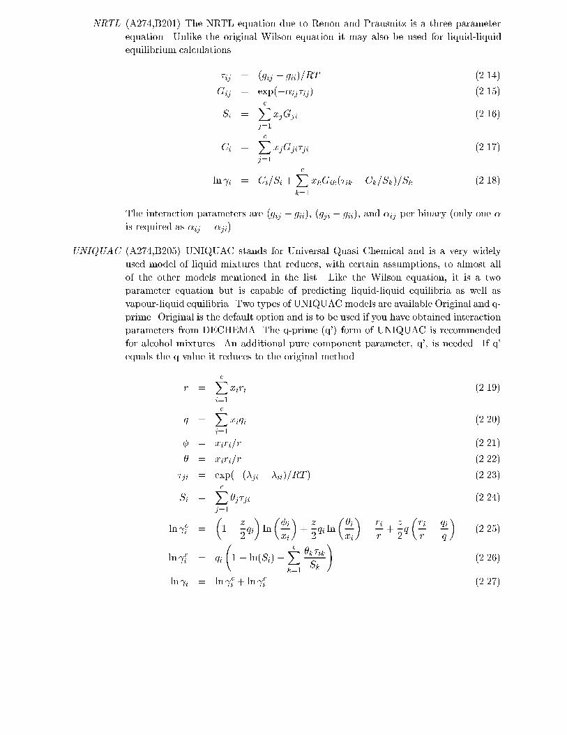
NRTL (A274,B201) The NRTL equation due to Renon and Prausnitz is a three parameter
equation. Unlike the original Wilson equation it may also be used for liquid-liquid
equilibrium calculations.
�ij = (gij � gii)=RT (2.14)
Gij = exp(��ij�ij) (2.15)
Si =cX
j=1
xjGji (2.16)
Ci =cX
j=1
xjGji�ji (2.17)
ln i = Ci=Si +cX
k=1
xkGik(�ik � Ck=Sk)=Sk (2.18)
The interaction parameters are (gij � gii), (gji � gii), and �ij per binary (only one �
is required as �ij = �ji).
UNIQUAC (A274,B205) UNIQUAC stands for Universal Quasi Chemical and is a very widely
used model of liquid mixtures that reduces, with certain assumptions, to almost all
of the other models mentioned in the list. Like the Wilson equation, it is a two
parameter equation but is capable of predicting liquid-liquid equilibria as well as
vapour-liquid equilibria. Two types of UNIQUAC models are available Original and q-
prime. Original is the default option and is to be used if you have obtained interaction
parameters from DECHEMA. The q-prime (q') form of UNIQUAC is recommended
for alcohol mixtures. An additional pure component parameter, q', is needed. If q'
equals the q value it reduces to the original method.
r =cX
i=1
xiri (2.19)
q =cX
i=1
xiqi (2.20)
� = xiri=r (2.21)
� = xiri=r (2.22)
�ji = exp(�(�ji � �ii)=RT ) (2.23)
Si =cX
j=1
�j�ji (2.24)
ln ci =
�1�
z
2qi
�ln
��i
xi
�+z
2qi ln
��i
xi
��ri
r+z
2q
�ri
r�qi
q
�(2.25)
ln ri = qi
1� ln(Si)�
cXk=1
�k�ik
Sk
!(2.26)
ln i = ln ci + ln ri (2.27)

y p
The interaction parameters are (�ij � �ii) and (�ji� �ii) per binary. The parametersri and qi are read from the component database (PCD �le).
UNIFAC (A314,B219) UNIFAC is a group contribution method that is used to predict equilibria
in systems for which NO experimental equilibrium data exist. The method is based
on the UNIQUAC equation, but is completely predictive in the sense that it does not
require interaction parameters. Instead, these are computed from group contributions
of all the molecules in the mixture. If you select one of the other models but fail to
specify a complete set of the interaction parameters, then UNIFAC is used to compute
any unspeci�ed parameters.
ASOG (A313,B219) ASOG is a group contribution method similar to UNIFAC but based on
the Wilson equation. It was developed before UNIFAC but is less widely used because
of the comparative lack of �tted group interaction parameters.
2.1.3 Vapour pressure models
Antoine (A208,B11) The Antoine Equation is:
lnP �i = Ai �
Bi
T + Ci(2.28)
Note the natural logarithm. This option should be selected if you are using activity
coe�cient models with parameters from the DECHEMA series. Antoine parameters
are available in the ChemSep data �les and need not be loaded.
Extended Antoine (B11) The Extended Antoine equation incorporated in ChemSep's thermodynamic
routines is:
lnP �i = Ai +
Bi
Ci + T+DiT +Ei lnT + FiT
G
i (2.29)
The parameters A through G must be supplied by the user. A library of parameters
for some common chemicals is provided with ChemSep in the �le EANTOINE.LIB.
DIPPR (B11) The Design Institute for Physical Property Research (DIPPR) has recently
published a correlation for the vapour pressure.
lnP �i = Ai +
Bi
T+DiT +Ci lnT +DiT
E
i (2.30)
DIPPR parameters A{E are also available in ChemSep data �les.
Riedel (B523) The Riedel equation is best suited to nonpolar mixtures:
�T = 36=Tr + 96:7 log Tr � 35� T 6r (2.31)
�Tb = 36=Trb + 96:7 log Trb � 35� T 6rb (2.32)
� = 0:118�T � 7 log Tr (2.33)
p p y
= 0:0364�T � log Tr (2.34)
� =0:136�Tb + logPc � 5:01
0:0364�Tb � log Trb(2.35)
logP �r = ��� (�� 7) (2.36)
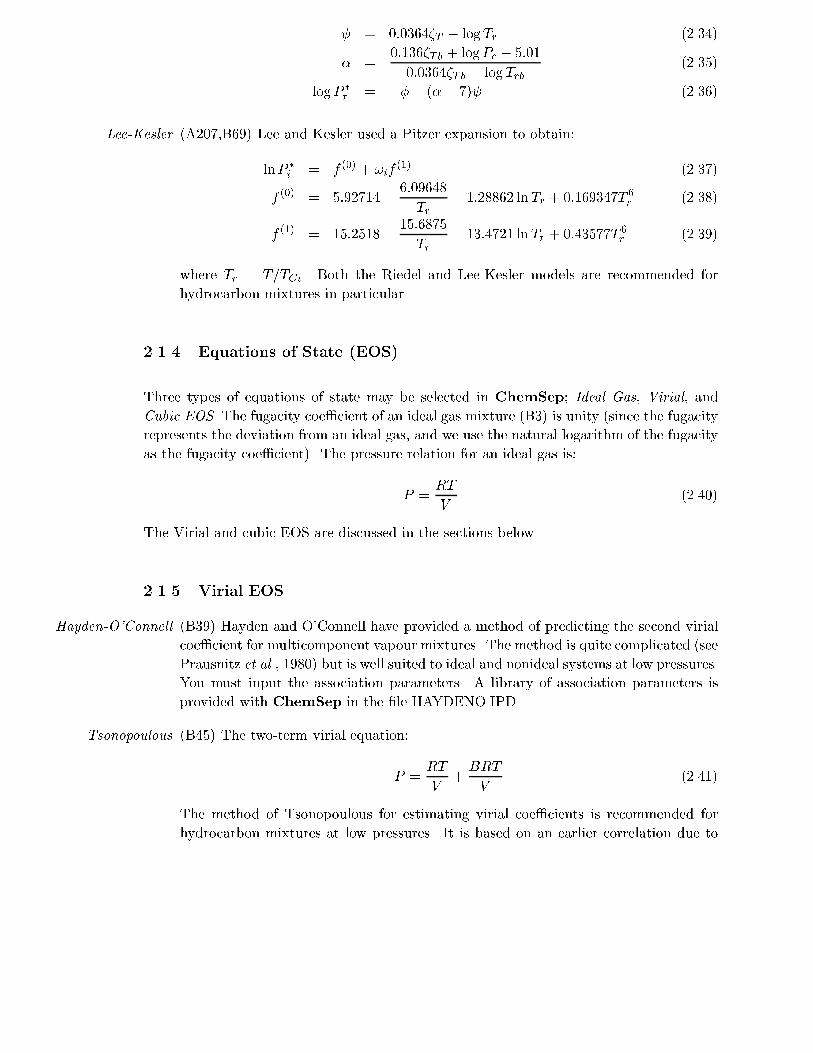
Lee-Kesler (A207,B69) Lee and Kesler used a Pitzer expansion to obtain:
lnP �i = f (0) + !if
(1) (2.37)
f (0) = 5:92714 �6:09648
Tr� 1:28862 ln Tr + 0:169347T 6
r (2.38)
f (1) = 15:2518 �15:6875
Tr� 13:4721 ln Tr + 0:43577T 6
r (2.39)
where Tr = T=TCi. Both the Riedel and Lee-Kesler models are recommended for
hydrocarbon mixtures in particular.
2.1.4 Equations of State (EOS)
Three types of equations of state may be selected in ChemSep; Ideal Gas, Virial, and
Cubic EOS. The fugacity coe�cient of an ideal gas mixture (B3) is unity (since the fugacity
represents the deviation from an ideal gas, and we use the natural logarithm of the fugacity
as the fugacity coe�cient). The pressure relation for an ideal gas is:
P =RT
V(2.40)
The Virial and cubic EOS are discussed in the sections below.
2.1.5 Virial EOS
Hayden-O'Connell (B39) Hayden and O'Connell have provided a method of predicting the second virial
coe�cient for multicomponent vapour mixtures. The method is quite complicated (see
Prausnitz et al., 1980) but is well suited to ideal and nonideal systems at low pressures.
You must input the association parameters. A library of association parameters is
provided with ChemSep in the �le HAYDENO.IPD.
Tsonopoulous (B45) The two-term virial equation:
P =RT
V+BRT
V(2.41)
The method of Tsonopoulous for estimating virial coe�cients is recommended for
hydrocarbon mixtures at low pressures. It is based on an earlier correlation due to

y p
Pitzer.
B =cX
i=1
cXj=1
yiyjBij (2.42)
Bij = RTc;ij Pc;ij
�B(0)ij
+ !ijB(0)ij
�(2.43)
B(0)ij
= 0:1445 �0:33
Tr�0:1385
T 2r
�0:0121
T 3r
�0:000607
T 8r
(2.44)
B(1)ij
= 0:0637 +0:331
T 2r
�0:423
T 3r
�0:0008T 8r
(2.45)
!ij =!i + !j
2(2.46)
Zc;ij =Zci + Zcj
2(2.47)
V1=3c;ij
=V1=3ci
V1=3cj
2(2.48)
Tc;ij = (1� kij)qTciTcj (2.49)
Pc;ij =Zc;ijRTc;ij
Vc;ij(2.50)
Binary interaction parameters kij must be supplied by the user. For para�ns kij can
be calculated with:
kij = 1�8pVciVcj
(V1=3ci
+ V c1=3cj
)3(2.51)
DIPPR The Design Institute for Physical Property Research (DIPPR) has published a cor-
relation for the second virial coe�cient, see the section on physical properties below.
The parameters for the DIPPR correlation are also available in ChemSep (PCD)
data �les.
Chemical theory This is an extension on the Hayden O'Connell virial model, which takes the association
of molecules into account (see Prausnitz et al., 1980). Since the mole fractions are
a function of the association, an iterative method (here Newton's method) must be
used to obtain them in order to compute the virial coe�cients.
2.1.6 Cubic EOS
Van der Waals (A43,B15) The Van der Waals (VdW) Equation was the �rst cubic equation of state.
The basic equation has served as a starting point for many other EOS. The VdW
equation cannot be used to determine properties of liquid phases, thus it may not be
selected for the EOS K-value model.
P =RT
V � b�
a
V 2(2.52)

p p y
with
ai =27R2T 2
ci
64Pci(2.53)
bi =RTci
8Pci(2.54)
and the mixing rules:
a =cX
i=1
cXj=1
yiyjaij (2.55)
aij =paiaj (2.56)
b =cX
i=1
yibi (2.57)
Redlich Kwong (A43,B43) The Redlich Kwong (RK) equation is used in the Chao-Seader method of
computing thermodynamic properties. The RK equation cannot be used to determine
properties of liquid phases, thus it cannot be selected for the EOS K-value model.
P =RT
V � b�
apTV (V + b)
(2.58)
with
ai =aR
2T 2:5ci
Pci(2.59)
a = 0:42748 (2.60)
bi =bRTci
Pci(2.61)
b = 0:08664 (2.62)
and the mixing rules:
a =cX
i=1
cXj=1
yiyjaij (2.63)
aij = (1� kij)paiaj (2.64)
b =cX
i=1
yibi (2.65)
where kij is a binary interaction parameter (original RK: kij = 0).
Soave Redlich Kwong (A43,B52) Soave's modi�cation of the Redlich Kwong (SRK) EOS is one of the most
widely used methods of computing thermodynamic properties. The SRK EOS is most
suitable for computing properties of hydrocarbon mixtures.
P =RT
V � b�
a
V (V + b)(2.66)

y p
with
ai = ai(Tci)�(Tri; !i) (2.67)
ai(Tci) =aR
2T 2ci
Pci(2.68)
a = 0:42747 (2.69)
�(Tri; !i) =h1 + (0:480 + 1:574!i � 0:176!2i )(1�
pTri)
i2(2.70)
bi =bRTci
Pci(2.71)
b = 0:08664 (2.72)
and the mixing rules:
a =cX
i=1
cXj=1
yiyjaij (2.73)
aij = (1� kij)paiaj (2.74)
b =cX
i=1
yibi (2.75)
API SRK EOS (B53) Graboski and Daubert have modi�ed the coe�cients in the SRK EOS and
provided a special relation for hydrogen. This modi�cation of the SRK EOS has been
recomended by the American Petroleum Institute (API), hence the name of this menu
option. It uses the same equations as the SRK except for the �:
�(Tri; !i) =h1 + (0:48508 + 1:55171!i � 0:15613!2i )(1�
pTri)
i2(2.76)
and specially for hydrogen:
�(Tri; !i) = 1:202e�0:30288Tri (2.77)
Peng Robinson EOS (A43,B54) The Peng-Robinson equation is another cubic EOS that owes its origins to
the RK and SRK EOS. The PR EOS, however, gives improved predictions of liquid
phase densities.
P =RT
V � b�
a
V (V + b) + b(V � b)(2.78)
with
ai = ai(Tci)�(Tri; !i) (2.79)
ai(Tci) =aR
2T 2ci
Pci(2.80)
a = 0:45724 (2.81)
�(Tri; !i) =h1 + (0:37464 + 1:5422!i � 0:26992!2i )(1 �
pTr)i2
(2.82)
bi =bRTci
Pci(2.83)
b = 0:07880 (2.84)

p p y
and the mixing rules:
a =cX
i=1
cXj=1
yiyjaij (2.85)
aij = (1� kij)paiaj (2.86)
b =cX
i=1
yibi (2.87)
2.1.7 Enthalpy
None No enthalpy balance is used in the calculations. WARNING: the use of this model
with subcooled and superheated feeds or for columns with heat addition or removal
on some of the stages will give incorrect results. The heat duties of the condenser and
reboiler will be reported as zero since there is no basis for calculating them.
Ideal (B152) In this model the enthalpy is computed from the ideal gas contribution. For
liquids, the latent heat of vaporization is subtracted from the ideal gas contribution.
Excess (B518) This model includes the ideal enthalpy as above. The excess enthalpy is
calculated from the activity coe�cient model or the temperature derivative of the
fugacity coe�cients dependent on the choice of the model for the K-values, and is
added to the ideal part.
Polynomial Vapour as well as liquid enthalpy are calculated as functions of the absolute temper-
ature (K). Both the enthalpies use the following function:
Hi = Ai +BiT + CiT2 +DiT
3 (2.88)
You must enter the coe�cients A through E in the "Load Data" option of the Prop-
erties menu for vapour and liquid enthalpy for each component.
2.2 Physical Properties
A number of di�erent polynomials is implemented in ChemSep to evaluate physical prop-
erties over a certain temperature range. These temperature correlations are assigned a
unique number in the range of 0-255 (see Table 2.1). For each up to 5 parameters (A-
E) are available. Table 2.2 shows which pure component properties can be modeled with
temperature correlations and their typical correlation number.
All types of equations may be used for any of the physical properties but, of course, some
formulas were speci�cally developed for prediction of particular properties. Besides the
parameters A-E the temperature limits of the correlation must also be present. If the
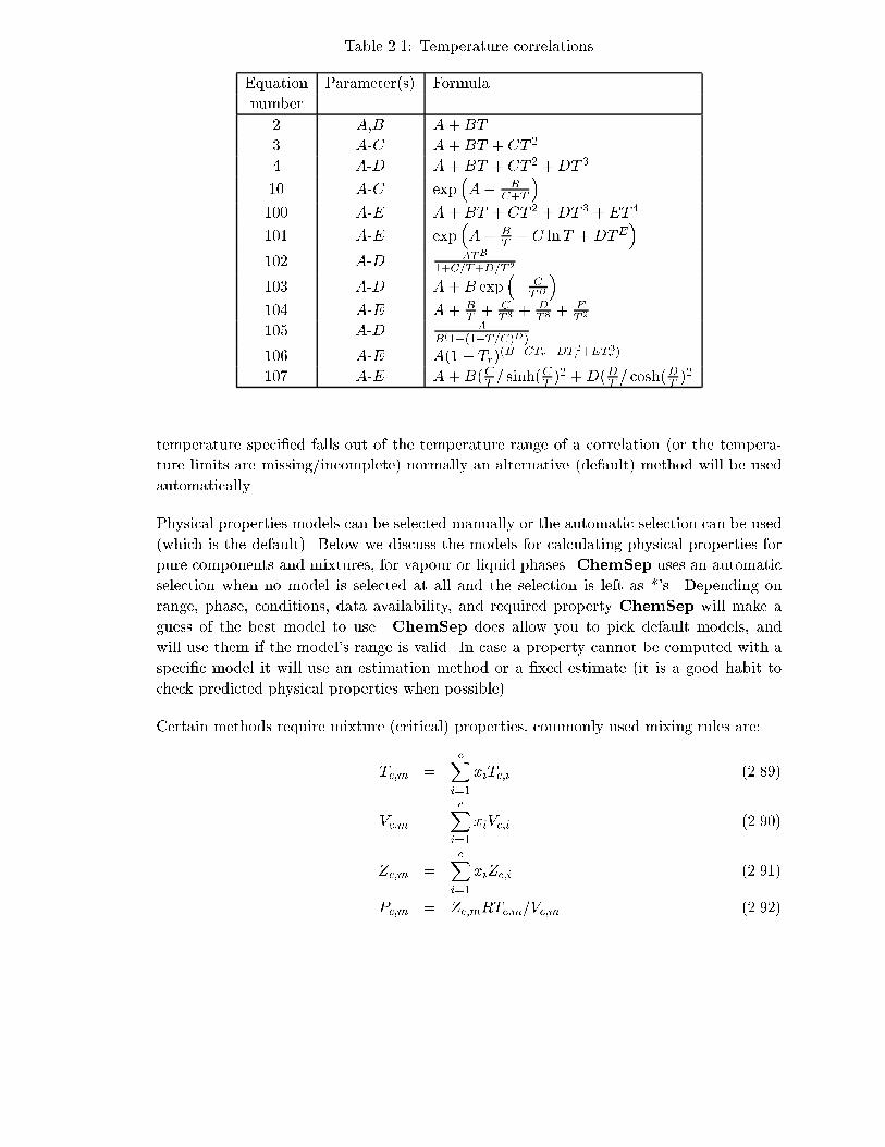
y p
Table 2.1: Temperature correlations
Equation Parameter(s) Formula
number
2 A,B A+BT
3 A-C A+BT + CT 2
4 A-D A+BT + CT 2 +DT 3
10 A-C exp�A� B
C+T
�100 A-E A+BT + CT 2 +DT 3 +ET 4
101 A-E exp�A+ B
T+C lnT +DTE
�102 A-D AT
B
1+C=T+D=T 2
103 A-D A+B exp�� C
TD
�104 A-E A+ B
T+ C
T 3 +D
T 8 +E
T 9
105 A-D A
B(1+(1�T=C)D)
106 A-E A(1� Tr)(B+CTr+DT 2
r+ET3r )
107 A-E A+B(CT= sinh(C
T)2 +D(D
T= cosh(D
T)2
temperature speci�ed falls out of the temperature range of a correlation (or the tempera-
ture limits are missing/incomplete) normally an alternative (default) method will be used
automatically.
Physical properties models can be selected manually or the automatic selection can be used
(which is the default). Below we discuss the models for calculating physical properties for
pure components and mixtures, for vapour or liquid phases. ChemSep uses an automatic
selection when no model is selected at all and the selection is left as *'s. Depending on
range, phase, conditions, data availability, and required property ChemSep will make a
guess of the best model to use. ChemSep does allow you to pick default models, and
will use them if the model's range is valid. In case a property cannot be computed with a
speci�c model it will use an estimation method or a �xed estimate (it is a good habit to
check predicted physical properties when possible).
Certain methods require mixture (critical) properties, commonly used mixing rules are:
Tc;m =cX
i=1
xiTc;i (2.89)
Vc;m =cX
i=1
xiVc;i (2.90)
Zc;m =cX
i=1
xiZc;i (2.91)
Pc;m = Zc;mRTc;m=Vc;m (2.92)
p p y
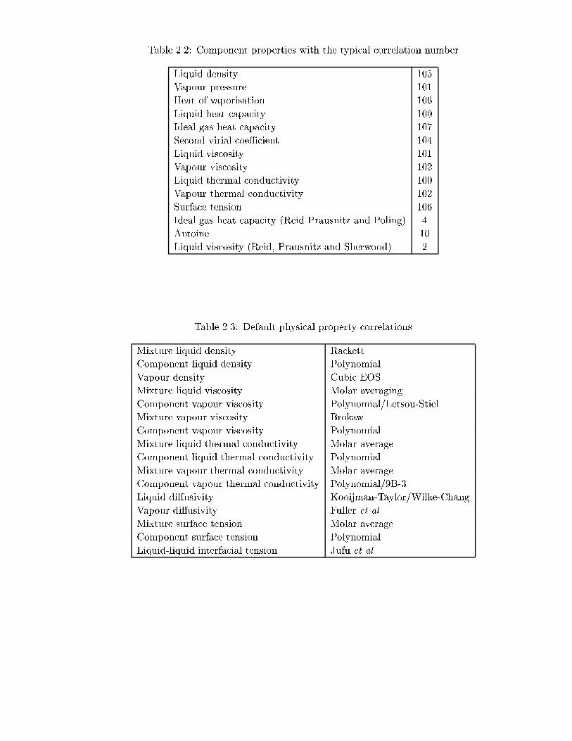
Table 2.2: Component properties with the typical correlation number
Liquid density 105
Vapour pressure 101
Heat of vaporisation 106
Liquid heat capacity 100
Ideal gas heat capacity 107
Second virial coe�cient 104
Liquid viscosity 101
Vapour viscosity 102
Liquid thermal conductivity 100
Vapour thermal conductivity 102
Surface tension 106
Ideal gas heat capacity (Reid Prausnitz and Poling) 4
Antoine 10
Liquid viscosity (Reid, Prausnitz and Sherwood) 2
Table 2.3: Default physical property correlations
Mixture liquid density Rackett
Component liquid density Polynomial
Vapour density Cubic EOS
Mixture liquid viscosity Molar averaging
Component vapour viscosity Polynomial/Letsou-Stiel
Mixture vapour viscosity Brokaw
Component vapour viscosity Polynomial
Mixture liquid thermal conductivity Molar average
Component liquid thermal conductivity Polynomial
Mixture vapour thermal conductivity Molar average
Component vapour thermal conductivity Polynomial/9B-3
Liquid di�usivity Kooijman-Taylor/Wilke-Chang
Vapour di�usivity Fuller et al.
Mixture surface tension Molar average
Component surface tension Polynomial
Liquid-liquid interfacial tension Jufu et al.

y p
Mm =cX
i=1
xiMi (2.93)
which will be referred as the "normal" mixing rules. Reduced properties will be calculated
by:
Tr = T=Tc (2.94)
Pr = P=Pc (2.95)
Vr = V=Vc (2.96)
unless speci�ed otherwise.
2.2.1 Liquid density
Mixture liquid densities (in kmol=m3) are calculated with:
Equation of State The previously discussed Peng-Robinson equation of state is used to calculate the
mixture compressibility directly from pure component critical properties and mixture
parameters, from which the density can be calculated easily. Use this method if some
components in the mixture are supercritical.
Amagat's law
1
�Lm=
cXi=1
xi
�Li
(2.97)
where the component liquid densities, �Li, are computed as discussed below.
Rackett (A67,89) This is DIPPR procedure 4B, which requires component critical tempera-
tures, pressures, mole weights and Racket parameters (for which critical compressibil-
ities are used if unknown):
Tc;m =cX
i=1
xiTc;i (2.98)
ZR;m =cX
i=1
xiZR;i (2.99)
Tr =T
Tc;m(2.100)
Fz = Z(1+(1�Tr)2=7)R;m
(2.101)
A =cX
i=1
xiTc;i
MiPc;i(2.102)
�Lm = 1=ARFz
cXi=1
xiMi (2.103)

p p y
If the reduced temperature, Tr, is greater than unity a default value of 50 kmol=m3
is used.
Yen-Woods Mixture critical temperature, volume, and compressibility are calculated with the
"normal" mixing rules. If the reduced temperature, Tr = T=Tc;m, is greater than
unity a default value of 50 kmol=m3 is used, otherwise the density is calculated from:
T� = (1� Tr)1=3 (2.104)
A = 17:4425 � 214:578Zc + 989:625 � Z2c � 1522:06Z3
c (2.105)
Zc � 0:26 : B = �3:28257 + 13:6377Zc + 107:4844Z2c � 384:211Z3
c (2.106)
Zc > 0:26 : B = 60:20901 � 402:063Zc + 501Z2c + 641Z3
c (2.107)
�Lm =1 +AT� +BT 2
� + (0:93 �B)T 4�
Vc(2.108)
Hankinson-Thompson (A55-66,89,90) Calculate mixture density by the methods of Hankinson and Thomson
(AIChE J, 25, 653, 1979) and Thomson et al. (AIChE J, 28, 671, 1982):
V �m =
1
4
cX
i=1
xiV�i + 3(
cXi=1
xiV�i
2=3)(cX
i=1
xiV�i
1=3)
!(2.109)
Tc;m =cXi=i
cXj=i
xixjV�ijTc;ij=V
�m (2.110)
!SRK;m =cX
i=1
xi!SRK;i (2.111)
Zc;m = 0:291 � 0:08!SRK;i (2.112)
Pc;m = Zc;mRTc;m=V�m (2.113)
If the reduced temperature is larger than unity a default value of 50 kmol=m3 is used,
otherwise the saturated liquid volume (Vs) is calculated from:
Vs
V �m
= V(0)R
(1� !SRK;mV(�)R
) (2.114)
V(0)R
= 1 + a(1� Tr)1=3 + b(1� Tr)
2=3 + c(1� Tr) + d(1� Tr)4=3 (2.115)
V(�)R
=e+ fTr + gT 2
r + hT 3r
(Tr � 1:00001)(2.116)
where
a=-1.52816 e=-0.296123
b= 1.43907 f= 0.386914
c=-0.81446 g=-0.0427258
d= 0.190454 h=-0.0480645
The density equals the inverse of the liquid molar volume.
For the density of compressed liquids the saturated liquid volume is corrected (Thom-
son et al., AIChE J, 28, 671, 1982):
V = Vs
1� c ln
� + P
� + Pvpm
!(2.117)

y p
�=Pc = �1 + a(1� Tr)1=3 + b(1� Tr)
2=3 + d(1 � Tr) + e(1� Tr)4=3 (2.118)
e = exp(f + g!SRK;m + h!2SRK;m (2.119)
c = j + k!SRK (2.120)
where
a=-9.070217 g= 0.250047
b= 62.45326 h= 1.14188
d=-135.1102 j= 0.0861488
f= 4.79594 k= 0.0344483
and the vapour pressure is from the generalized Riedel equations:
Pvpm = Pc;mPrm (2.121)
logPrm = P (0)rm + !SRK;mP
(1)rm (2.122)
P (0)rm = 5:8031817 log Trm + 0:07608141� (2.123)
P (1)rm = 4:86601 log Trm + 0:03721754� (2.124)
� = 35� 36=Trm � 96:736 log Trm + T 6rm (2.125)
Trm = T=Tc;m (2.126)
This method should be used for reduced temperatures from 0.25 up to the critical
point.
Pure component liquid densities are computed from the Peng-Robinson EOS for tempera-
tures above a components critical temperature, otherwise with one of the folowing methods:
Polynomial When within the temperature range, a polynomial is the default way for calculating
component liquid densities.
Rackett This is the DIPPR procedure 4A:
Fz = Z(1+(1�Tr)2=7)R
(2.127)
�Lm = Pc=RTcFz (2.128)
COSTALD Hankinson and Thompson method described as above but with pure component pa-
rameters.
The pure component liquid densities are corrected for pressure e�ects with the correction of
Thomson et al. (1982) as described for the Hankinson and Thompson method for mixtures.
2.2.2 Vapour density
Vapour densities are computed with the equation of state selected for the thermodynamic
properties (possible selections are Ideal gas EOS, Virial EOS, and Cubic EOS).

p p y
2.2.3 Liquid Heat Capacity
The mixture liquid heat capacity is the molar average of the component liquid heat ca-
pacities, which are generally computed from a temperature correlation. Alternatively the
liquid heat capacity could be computed from a corresponding states method and the ideal
gas capacity. Rowlinson (1969, see A140) proposed a Lee-Kesler heat capacity departure
function which was later modi�ed to:
CL
p;i � Cig
p = 1:45 + 0:45(1 � Tr)�1 + 0:25!
h17:11 + 25:2(1 � Tr)
1=3T�1r + 1:742(1 � Tr)�1i
(2.129)
However, in ChemSep the temperature correlation is used for all temperatures to prevent
problems arrising from using di�erent liquid heat capacity methods in the same column
(which especially trouble nonequilibrium models). Liquid heat capacities could also be
computed from the selected thermodynamic models to circumvent this problem.
2.2.4 Vapour Heat Capacity
The mixture vapour heat capacity is the molar average of the component vapour heat capac-
ities, which are computed from the ideal gas heat capacity (RPP) 4 parameter temperature
correlation. If no parameters for this correlation are present, the vapour heat capacity
temperature correlation is used (if within the temperature range).
2.2.5 Liquid Viscosity
Mixture liquid viscosity are computed from DIPPR procedure 8H from the pure component
liquid viscosities from:
ln �Lm =cX
i=1
zi ln�L
i (2.130)
where zi are either the mole fractions (for molar averaging, the default) or alternatively the
weight fractions for mass averaging. A better method is from Teja and Rice (1981, A479).
However, this method requires interaction parameters. Here a di�erent mixing rule (for
TcijVcij) is used which improves the model predictions with unity interaction coe�cients:
!m =cX
i=1
xi!i (2.131)
Mm =cX
i=1
xiMi (2.132)
Vcm =cX
i=1
cXj=1
xixjVcij (2.133)

y p
Vcij =
�V1=3ci
+ V1=3cj
�38
(2.134)
Tcm =
Pc
i=1
Pc
j=1 xixjTcijVcij
Vcm(2.135)
TcijVcij = ijTciVci + TcjVcj
2(2.136)
where ij is set to unity for all components. The liquid viscosity of the mixture is computed
from two reference components
ln(�m�m) = ln(�1�1) + [ln(�2�2)� ln(�1�1)]
�!m � !1
!2 � !1
�(2.137)
with � de�ned as
�i =V2=3cipTciMi
(2.138)
and the reference component vioscosities are evaluated at TTci=Tcm. Component liquid
viscosities are calculated from the liquid viscosity temperature correlation if the temperature
is within the valid range. Otherwise the component viscosity is computed with DIPPR
procedure 8G, the Letsou-Stiel method (1973, see A471):
� =2173:424T
1=6c;i
pMiP
2=3c;i
(2.139)
�(0) = (1:5174 � 2:135Tr + 0:75T 2r )10
�5 (2.140)
�(1) = (4:2552 � 7:674Tr + 3:4T 2r )10
�5 (2.141)
�Li = (�(0) + !�(1))=� (2.142)
Alternatively the simple temperature correlation given in Reid et al. (RPS liquid viscosity,
see A439) can be used:
log � = A+B=T (2.143)
A high pressure correction by Lucas (A436) is used to correct the in uence of the pressure
on the liquid viscosity:
� =1 +D(�Pr=2:118)
A
1 + C!i�Pr�SL (2.144)
where �SL is the viscosity of the saturated liquid at Pvp, and
�Pr = (P � Pvp)=Pci (2.145)
A = 0:9991 � [4:674 10�4=(1:0523T�0:03877r � 1:0513)] (2.146)
C = �0:07921 + 2:1616Tr � 13:4040T 2r + 44:1706T 3
r (2.147)
�84:8291T 4r + 96:1209T 5
r � 59:8127T 6r + 15:6719T 7
r (2.148)
D = [0:3257=(1:0039 � T 2:573r )0:2906]� 0:2086 (2.149)
p p y
2.2.6 Vapour Viscosity
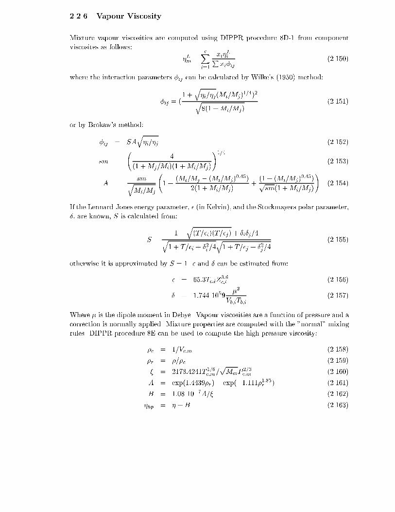
Mixture vapour viscosities are computed using DIPPR procedure 8D-1 from component
viscosites as follows:
�Lm =cX
i=1
xi�LiP
xi�ij(2.150)
where the interaction parameters �ij can be calculated by Wilke's (1950) method:
�ij = (1 +
q�i=�j(Mi=Mj)
1=4)2q8(1 +Mi=Mj)
(2.151)
or by Brokaw's method:
�ij = SAq�i=�j (2.152)
sm =
4
(1 +Mj=Mi)(1 +Mi=Mj)
!1=4
(2.153)
A =smqMi=Mj
1 +
(Mi=Mj � (Mi=Mj)0:45)
2(1 +Mi=Mj)+(1 + (Mi=Mj)
0:45)psm(1 +Mi=Mj)
!(2.154)
If the Lennard-Jones energy parameter, � (in Kelvin), and the Stockmayers polar parameter,
�, are known, S is calculated from:
S =1 +
q(T=�i)(T=�j) + �i�j=4q
1 + T=�i + �2i=4q1 + T=�j + �2
j=4
(2.155)
otherwise it is approximated by S = 1. � and � can be estimated from:
� = 65:3Tc;iZ3:6c;i (2.156)
� = 1:744 1059�2
Vb;iTb;i(2.157)
Where � is the dipole moment in Debye. Vapour viscosities are a function of pressure and a
correction is normally applied. Mixture properties are computed with the "normal" mixing
rules. DIPPR procedure 8E can be used to compute the high pressure viscosity:
�c = 1=Vc;m (2.158)
�r = �=�c (2.159)
� = 2173:4241T 1=6c;m =
pMmP
2=3c;m (2.160)
A = exp(1:4439�r)� exp(�1:111�1:85r ) (2.161)
B = 1:08 10�7A=� (2.162)
�hp = � +B (2.163)

y p
Table 2.4: Constants for the Yoon-Thodos method
Hydrogen Helium Others
a=47.65 a=52.57 a=46.1
b=0.657 b=0.656 b=0.618
c=20.0 c=18.9 c=20.4
d=-0.858 d=-1.144 d=-0.449
e=19.0 e=17.9 e=19.4
f=-3.995 f=-5.182 f=-4.058
where � is the vapour mixture molar density.
Both Wilke's and Brokaw's method require pure component viscosities. These are normally
obtained from the vapour viscosity temperature correlations, as long as the temperature is
within the valid temperature range. If not, then the viscosity can be computed with the
Chapman-Enskog kinetic theory (see Hirschfelder et al. 1954 and A391-393):
T � = T=� (2.164)
v = a(T �)�b + c= exp(dT �) + e= exp(fT �) (2.165)
�V = 26:69 10�7MT=�2(v + 0:2�2=T �) (2.166)
where the collision integral constants are a = 1:16145, b = 0:14874, c = 0:52487, d =
0:77320, e = 2:16178, and f = 2:43787. The viscosity may also be computed with the Yoon
and Thodos method (DIPPR procedure 8B):
�i = 2173:4241T1=6c;i
=pMiP
2=3c;i
(2.167)
�Vi =1 + aT b
r � c exp(dT � r) + e exp(fTr)
108�(2.168)
where the constants a� f are given in Table 2.4.
Another method for calculating the vapor viscosity is the Lucas (A397) method:
� = 10�7[0:807T 0:618r � 0:357 exp(�0:449Tr) + (2.169)
0:340 exp(�4:058Tr) + 0:018]F o
p Fo
q =� (2.170)
� = 0:176
�Tc
M3(10�5Pc)4
�1=6(2.171)
where F op and F o
q are polarity and quantum correction factors. The polarity correction
depends on the reduced dipole moment:
�r = 52:46(�=3:336 10�30)2(10�5Pc)
T 2c
(2.172)

p p y
If �r is smaller than 0.022 then the correction factor is unity, else if it is smaller than 0.075
it is given by
F o
p = 1 + 30:55(0:292 � Zc)1:72 (2.173)
else by
F o
p = 1 + 30:55(0:292 � Zc)1:72[0:96 + 0:1(Tr � 0:7)] (2.174)
The quantum correction is only used for quantum gases He, H2, and D2,
F o
q = 1:22Q0:15�1 + 0:00385[(Tr � 12)2]1=Msign(Tr � 12)
�(2.175)
where Q = 1:38 (He), Q = 0:76 (H2), Q = 0:52 (D2). There is also a speci�c correction for
high pressures (A421) by Lucas.
� = Y FpFq�o (2.176)
Y = 1 +aP e
r
bPfr + (1 + cP d
r )�1
(2.177)
Fp =1 + (F o
p � 1)Y �3
F op
(2.178)
Fq =1 + (F o
q � 1)[Y �1 � 0:007(ln Y )4]
F oq
(2.179)
where �o refers to the low-pressure viscosity (note that the original Lucas method has a
di�erent rule for Y if Tr is below unity, however, this introduces a discontinuity which is
avoided here). The parameters a through f are evaluated with:
a =1:245 10�3
Trexp 5:1726T�0:3286r (2.180)
b = a(1:6553Tr � 1:2723) (2.181)
c =0:4489
Trexp 3:0578T�37:7332r (2.182)
d =1:7368
Trexp 2:2310T�7:6351r (2.183)
e = 1:3088 (2.184)
f = 0:9425 exp�0:1853T 0:4489r (2.185)
where, in case Tr is below unity, Tr is taken to be unity. For mixtures the Lucas model uses
the following mixing rules:
Tcm =cX
i=1
yiTci (2.186)
Vcm =cX
i=1
yiVci (2.187)
Zcm =cX
i=1
yiZci (2.188)
y p
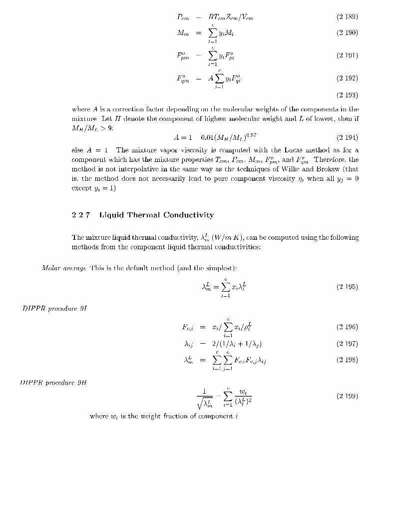
Pcm = RTcmZcm=Vcm (2.189)
Mm =cX
i=1
yiMi (2.190)
F o
pm =cX
i=1
yiFo
pi (2.191)
F o
qm = AcX
i=1
yiFo
qi (2.192)
(2.193)
where A is a correction factor depending on the molecular weights of the components in the
mixture. Let H denote the component of highest molecular weight and L of lowest, then if
MH=ML > 9:
A = 1� 0:01(MH=ML)0:57 (2.194)
else A = 1. The mixture vapor viscosity is computed with the Lucas method as for a
component which has the mixture properties Tcm, Pcm, Mm, Fopm, and F
oqm. Therefore, the
method is not interpolative in the same way as the techniques of Wilke and Brokaw (that
is, the method does not necessarily lead to pure component viscosity �i when all yj = 0
except yi = 1).
2.2.7 Liquid Thermal Conductivity
The mixture liquid thermal conductivity, �Lm (W=mK), can be computed using the following
methods from the component liquid thermal conductivities:
Molar average This is the default method (and the simplest):
�Lm =cX
i=1
xi�L
i (2.195)
DIPPR procedure 9I
Fv;i = xi=cX
i=1
xi=�L
i (2.196)
�ij = 2=(1=�i + 1=�j) (2.197)
�Lm =cX
i=1
cXj=1
Fv;iFv;j�ij (2.198)
DIPPR procedure 9H
1q�Lm
=cX
i=1
wi
(�Li)2
(2.199)
where wi is the weight fraction of component i.

p p y
A correction is applied when the pressure is larger than 3.5 bar:
�hp =�0:63T 1:2
r Pr=(30 + Pr) + 0:98 + 0:0079PrT1:4r
�� (2.200)
This is DIPPR procedure 9G-1 where the mixture parameters are computed by the "normal"
mixing rules. Component liquid thermal conductivities are calculated from one of the
following methods:
Polynomial The temperature correlation is normally used as long as the temperature is in the
valid range and no other method is explicitly selected.
Pachaiyappan et al.
f = 3 + 20(1 � Tr)2=3 (2.201)
b = 3 + 20(1 � 273:15=Tc;i)2=3 (2.202)
�i = c10�4Mx
i �L
i (f=b) (2.203)
for straight chain hydrocarbons c = 1:811 and x = 1:001 else c = 4:407 and x = 0:7717.
Latini et al. This is DIPPR procedure 9E (see A549,550):
�Li =A(1� Tr)
0:38
T1=6r
(2.204)
A =A�T�
b
M�
iT c
(2.205)
where parameters A�, �, �, and depend on the class of the component as shown in
Table 2.5.
2.2.8 Vapour Thermal Conductivity
Molar average The mixture vapour thermal conductivity is computed from the pure component ther-
mal conductivities as follows:
�Vm =cX
i=1
xi�V
i (2.206)
Kinetic theory This is DIPPR procedure 9D:
�Vm =cX
i=1
xi�ViP
c
j=1 xj�ij(2.207)
where interaction parameters �ij are computed from:
�ij = 0:25(1 +
vuut �i
�j
Mj
Mi
3=4 T + 1:5Tb;i
T + 1:5Tb;j)2T +
q1:52Tb;iTb;j
T + 1:5Tb;i(2.208)
Note that the component viscosities are required for this evaluation.

y p
Table 2.5: Parameters for the Latini equation for liquid thermal conductivity
Family A� � �
Saturated hydrocarbons 0.0035 1.2 0.5 0.167
Ole�ns 0.0361 1.2 1.0 0.167
Cyclopara�ns 0.0310 1.2 1.0 0.167
Aromatics 0.0346 1.2 1.0 0.167
Alcohols, phenols 0.00339 1.2 0.5 0.167
Acids (organic) 0.00319 1.2 0.5 0.167
Ketones 0.00383 1.2 0.5 0.167
Esters 0.0415 1.2 1.0 0.167
Ethers 0.0385 1.2 1.0 0.167
Refrigerants:
R20, R21, R22, R23 0.562 0.0 0.5 -0.167
Others 0.494 0.0 0.5 -0.167
If the system pressure is larger than 1 atmosphere a corection is applied according to
DIPPR procedure 9C-1. Mixture parameters are computed using the "normal" mixing
rules. Critical and reduced densities are computed from:
�c =1
Vc;m(2.209)
�r =�
�c(2.210)
If the reduced density is below 0:5 then a = 2:702, b = 0:535, and c = �1; if the reduceddensity is witin [0:5; 2] then a = 2:528, b = 0:67, and c = �1:069; otherwise a = 0:574,
b = 1:155, and c = 2:016. The high pressure thermal conductivity correction is then
calculated from:
�� =a10�8(exp(b�r) + c)�p
MmT1=6c;m
P2=3c;m
�Z5c;m
(2.211)
which must be added to the calculated thermal conductivity for low pressure.
Pure component vapour thermal conductivities are estimated from the following methods:
Polynomial The temperature correlation is normally used as long as the temperature is in the
valid range and no other method is explicitly selected.
DIPPR procedure 9B-3 This method is the default in case the temperature is out of the range of the temper-
ature correlation:
�Vi = (1:15(Cp �R) + 16903:36)�Vi =Mi (2.212)
p p y
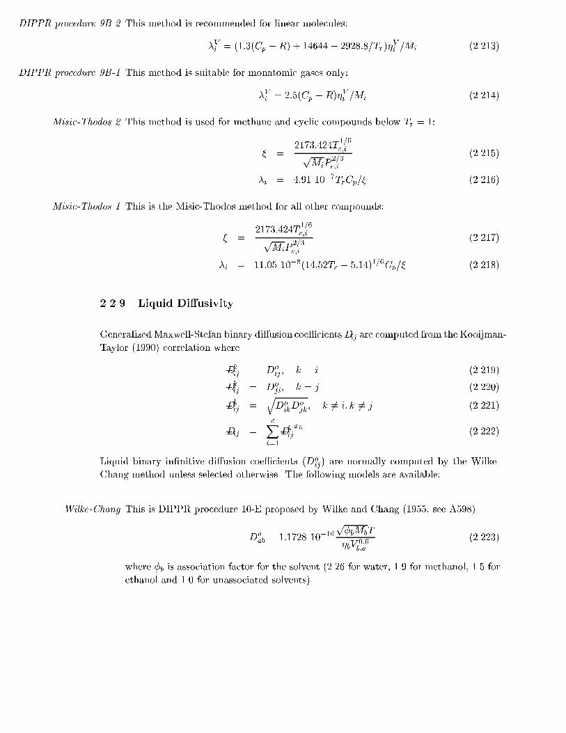
DIPPR procedure 9B-2 This method is recommended for linear molecules:
�Vi = (1:3(Cp �R) + 14644 � 2928:8=Tr)�V
i =Mi (2.213)
DIPPR procedure 9B-1 This method is suitable for monatomic gases only:
�Vi = 2:5(Cp �R)�Vi =Mi (2.214)
Misic-Thodos 2 This method is used for methane and cyclic compounds below Tr = 1:
� =2173:424T
1=6c;i
pMiP
2=3c;i
(2.215)
�i = 4:91 10�7TrCp=� (2.216)
Misic-Thodos 1 This is the Misic-Thodos method for all other compounds:
� =2173:424T
1=6c;i
pMiP
2=3c;i
(2.217)
�i = 11:05 10�8(14:52Tr � 5:14)1=6Cp=� (2.218)
2.2.9 Liquid Di�usivity
Generalized Maxwell-Stefan binary di�usion coe�cientsD�ij are computed from the Kooijman-
Taylor (1990) correlation where
D�k
ij = Do
ij ; k = i (2.219)
D�k
ij = Do
ji; k = j (2.220)
D�k
ij =qDo
ikDo
jk; k 6= i; k 6= j (2.221)
D�ij =cX
i=1
D�k
ij
xk(2.222)
Liquid binary in�nitive di�usion coe�cients (Doij) are normally computed by the Wilke-
Chang method unless selected otherwise. The following models are available:
Wilke-Chang This is DIPPR procedure 10-E proposed by Wilke and Chang (1955, see A598)
Do
ab = 1:1728 10�16p�bMbT
�bV0:6b;a
(2.223)
where �b is association factor for the solvent (2.26 for water, 1.9 for methanol, 1.5 for
ethanol and 1.0 for unassociated solvents).

y p
Hayduk-Laudie This is DIPPR procedure 10-F for the di�usivity of solute a in water proposed by
Hayduk and Laudie (1974)
Do
aw = 8:62 10�14��1:14w V �0:589b;a
(2.224)
Hayduk-Minhas aqueous Estimates di�usivity of solute a in water, proposed by Hayduk and Minhas (1982, see
also A602):
Do
aw = (3:36V �0:19b;a
� 3:65)10�13(1000�w)(0:00958=Vb;a�1:12)T 1:52 (2.225)
Hayduk-Minhas for non-aqueous systems Estimates di�usivity of solute a in polar and non-polar sol-
vent b (which is not water), proposed by Hayduk and Minhas (1982, see also A603):
Do
ab = 4:3637 10�18��0:19b
r0:2a r�0:4b
T 1:7 (2.226)
Hayduk-Minhas para�ns Estimates di�usion coe�cients for mixtures of normal para�ns from Hayduk-Minhas
correlation equation 7 of their paper as corrected by Siddiqi and Lucas (1986, see also
A602):
Do
ab = 9:859 10�14V �071b;a
(1000�b)(0:0102=Vb;a�0791) (2.227)
Siddiqi-Lucas aqueous Estimates di�usivity of solute a in water, proposed by Siddiqi and Lucas (1986):
Do
aw = 5:6795 10�16V �0:5473b;a
��1:026w T (2.228)
Siddiqi-Lucas Estimates di�usivity of solute a in solvent b (not water), proposed by Siddiqi and
Lucas (1986):
Do
ab = 5:2383 10�15V �0:45b;a
V 0:265b;b ��0:907
bT (2.229)
Umesi-Danner Estimates di�usivity of solute a in solvent b:
Do
ab = 5:927 10�12Trb
�br2=3a
(2.230)
Tyn-Calus correlation Estimates di�usivity of solute a in solvent b (see A600):
Do
ab = 8:93 10�12 Vb;a
V 2b;b
!1=6 �Pb
Pa
�0:6 T�b
(2.231)
This method is not yet implemented!

p p y
Table 2.6: Fuller di�usion volumes
Atomic and structural di�usion volume increments
C 15.9 F 14.7
H 2.31 Cl 21.0
O 6.11 Br 21.9
N 4.54 I 29.8
Ring -18.3 S 22.9
Di�usion volumes of simple molecules
He 2.67 CO 18.0
Ne 5.98 CO2 26.9
Ar 16.2 N2O 35.9
Kr 24.5 NH3 20.7
Xe 32.7 H2O 13.1
H2 6.12 SF6 71.3
D2 6.84 Cl2 38.2
N2 18.5 Br2 69.0
O2 16.3 SO2 41.8
Air 19.7
2.2.10 Vapour Di�usivity
Generalized Maxwell-Stefan binary di�usion coe�cients Dij are equal to the normal binary
di�usion coe�cients (since the gas is considered an ideal system for which the thermo-
dynamic matrix is the identity matrix). Normally these are computed with the Fuller-
Schettler-Giddings method (see A587) but if Fuller volume parameters are missing the
Wilke-Lee modi�cation of the Chapman-Enskog kinetic theory is used.
Fuller et al. This is DIPPR procedure 10-A which was developed by Fuller et al. (1966,1969):
DV
ab = 1:013 10�2T 1:75
p(1=Ma + 1=Mb)
P ( 3pVa +
3pVb)2
(2.232)
where Va and Vb are the Fuller molecular di�usion volumes which are calculated by
summing the atomic contributions from Table 2.6. This table also lists some special
di�usion volumes for simple molecules.
Chapman-Enskog This is DIPPR procedure 10B which computes the binary gas di�usion coe�cient
from a simpli�ed kinetic theory correlation. The average collision diameter and energy
parameter are:
�ab = (�a + �b)=2 (2.233)
�ab =p�a + �b (2.234)

y p
The di�suion collision integral is
T � = T=�ab (2.235)
D = a(T �)�b + c= exp(dT �) + e= exp(fT �) + g= exp(hT �) (2.236)
where the collision integral constants are a = 1:06036, b = 0:1561, c = 0:193, d =
0:47635, e = 1:03587, f = 1:52996, g = 1:76474, and h = 3:89411. If Stockmayer
polar parameters are known the integral gets corrected with:
D;c = D +0:19�a�b
T �(2.237)
and the di�usion coe�cient is
DV
ab = CT 3=2sqrt1=Ma + 1=Mb
P�ab!D(2.238)
where constant C = 1:883 10�2.
Wilke-Lee Wilke and Lee (1955, see A587) proposed modi�ed version of the kinetic theory
method described above with
C = 2:1987 10�2 � 5:07 10�3q1=Ma + 1=Mb (2.239)
2.2.11 Surface Tension
Mixture:
Molar avarage This is the default method:
�m =cX
i=1
xi�i (2.240)
Winterfeld et al. This method by Winterfeld et al. (1978) is DIPPR 7C procedure:
�m =
Pc
i=1
�(xi=�
Li)2 +
Pc
j=1(xixjp�i�j=�
Li�Lj)�
�Pc
i=1(xi=�Li)�2 (2.241)
Digulio-Teja This method evaluates the component surface tensions at the components normal
boiling points (�b;i) and computes the mixture critical temperature, normal boiling
temperature and the mixture surface tension at normal boiling temperature with the
following mixing rules:
Tc;m =cX
i=1
xiTc;i (2.242)
Tb;m =cX
i=1
xiTb;i (2.243)
�b;m =cX
i=1
xi�b;i (2.244)
p p y
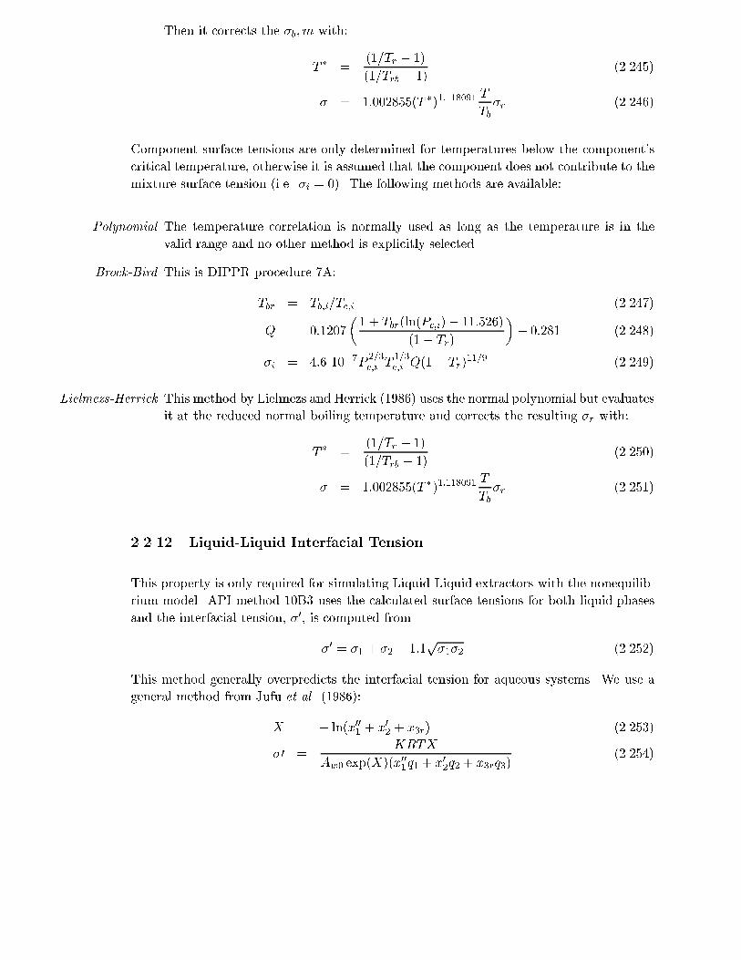
Then it corrects the �b;m with:
T � =(1=Tr � 1)
(1=Trb � 1)(2.245)
� = 1:002855(T �)1:118091T
Tb�r (2.246)
Component surface tensions are only determined for temperatures below the component's
critical temperature, otherwise it is assumed that the component does not contribute to the
mixture surface tension (i.e. �i = 0). The following methods are available:
Polynomial The temperature correlation is normally used as long as the temperature is in the
valid range and no other method is explicitly selected.
Brock-Bird This is DIPPR procedure 7A:
Tbr = Tb;i=Tc;i (2.247)
Q = 0:1207
�1 + Tbr(ln(Pc;i)� 11:526)
(1� Tr)
�� 0:281 (2.248)
�i = 4:6 10�7P2=3c;i
T1=3c;i
Q(1� Tr)11=9 (2.249)
Lielmezs-Herrick This method by Lielmezs and Herrick (1986) uses the normal polynomial but evaluates
it at the reduced normal boiling temperature and corrects the resulting �r with:
T � =(1=Tr � 1)
(1=Trb � 1)(2.250)
� = 1:002855(T �)1:118091T
Tb�r (2.251)
2.2.12 Liquid-Liquid Interfacial Tension
This property is only required for simulating Liquid-Liquid extractors with the nonequilib-
rium model. API method 10B3 uses the calculated surface tensions for both liquid phases
and the interfacial tension, �0, is computed from
�0 = �1 + �2 � 1:1p�1�2 (2.252)
This method generally overpredicts the interfacial tension for aqueous systems. We use a
general method from Jufu et al. (1986):
X = � ln(x001 + x02 + x3r) (2.253)
�0 =KRTX
Aw0 exp(X)(x001q1 + x02q2 + x3rq3)(2.254)

with Aw0 = 2:5 105 (m2=mol), R = 8:3144 (J=mol=K), K = 0:9414 (�), and qi is the
UNIQUAC surface area parameters of the components i. The components are ordered in
such a manner that component 1 and 2 are the dominating components in the two liquid
phases. Then the rest of the components are lumped into one mole fraction, x3. This
lumped mole fraction is taken for the phase which has the largest x3 (the richest). q3 is the
molar averaged q for that phase for all components except 1 and 2.
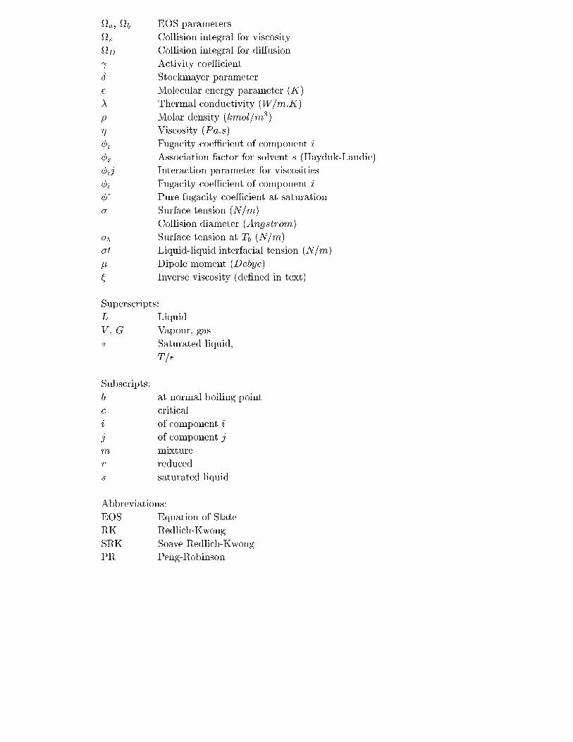
Symbol List
a, b Cubic EOS parameters
B Second virial coe�cient (m3=kmol)
c Number of components
Cp Mass heat capacity (J=kg:K)
Dij Binary di�usion coe�cient (m2=s)
D�ij Binary Maxwell-Stafan di�usion coe�cient (m2=s)
Doij
In�nite dilution binary di�usion coe�cient (m2=s)
Ki K-value of component i, equilibrium ratio (Ki = yi=xi)
kij Binary interaction coe�cient (for EOS)
M Molecular mass (kg=kmol)
R Gas constant = 8134 (J=kmolK)
r Radius of gyration (Angstrom)
P Pressure (Pa)
P �, Pvap Vapour pressure (Pa)
Pi Parachor (m3kg1=4=s1=2) of component i
PF Poynting correction
q UNIQUAC surface area parameter
T Temperature (K)
Tr Reduced temperature (Tr = T=Tc)
Tb Normal boiling temperature (K)
V Molar volume (m3=kmol)
Vb Molar volume at normal boiling point (m3=kmol)
Vs Saturated molar volume (m3=kmol)
w Weight fraction (of component)
x Liquid mole fraction (of component)
y Vapour mole fraction (of component)
Z Compressibility
ZR Racket parameter
Greek:
� Attractive parameter in EOS
! Acentric factor
p p y
a, b EOS parameters
v Collision integral for viscosity
D Collision integral for di�usion
Activity coe�cient
� Stockmayer parameter
� Molecular energy parameter (K)
� Thermal conductivity (W=m:K)
� Molar density (kmol=m3)
� Viscosity (Pa:s)
�i Fugacity coe�cient of component i
�s Association factor for solvent s (Hayduk-Laudie)
�ij Interaction parameter for viscosities
�i Fugacity coe�cient of component i
�� Pure fugacity coe�cient at saturation
� Surface tension (N=m)
Collision diameter (Angstrom)
�b Surface tension at Tb (N=m)
�0 Liquid-liquid interfacial tension (N=m)
� Dipole moment (Debye)
� Inverse viscosity (de�ned in text)
Superscripts:
L Liquid
V , G Vapour, gas
� Saturated liquid,
T=�
Subscripts:
b at normal boiling point
c critical
i of component i
j of component j
m mixture
r reduced
s saturated liquid
Abbreviations:
EOS Equation of State
RK Redlich-Kwong
SRK Soave Redlich-Kwong
PR Peng-Robinson

References
Digulio, Teja, Chem. Eng. J., Vol. 38 (1988) pp. 205.
E.N. Fuller, K. Ensley, J.C. Giddings, \A New Method for Prediction of Binary Gas-Phase
Di�usion Coe�cients", Ind. Eng. Chem., Vol. 58, (1966) pp. 19{27.
E.N. Fuller, P.D. Schettler, J.C. Giddings, \Di�usion of Halogonated Hydrocarbons in He-
lium. The E�ect of Structure on Collision Cross sections", J. Phys. Chem., Vol. 73 (1969)
pp. 3679{3685.
W. Hayduk, H. Laudie, \Prediction of Di�usion Coe�cients for Nonelectrolytes in Dilute
Aqueous Solutions", AIChE J., Vol. 20, (1974) pp. 611{615.
W. Hayduk, B.S. Minhas, \Correlations for Prediction of Molecular Di�usivities in Liquids",
Can. J. Chem. Eng., 60, 295-299 (1982); Correction, Vol. 61, (1983) pp. 132.
J.O. Hirschfelder, C.F. Curtis, R.B. Bird, Molecular Theory of Gases and Liquids, Wiley,
New York (1954).
F. Jufu, L. Buqiang, W. Zihao, \Estimation of Fluid-Fluid Interfacial Tensions of Multi-
component Mixtures", Chem. Eng. Sci., Vol. 41, No. 10 (1986) pp. 2673{2679.
R. Taylor, H.A. Kooijman, \Composition Derivatives of Activity Coe�cient Models (For
the estimation of Thermodynamic Factors in Di�usion)", Chem. Eng. Comm., Vol. 102,
(1991) pp. 87{106.
A. Letsou, L.I. Stiel, AIChE J., Vol. 19 (1973) pp. 409.
Lielmezs, Herrick, Chem. Eng. J., Vol. 32 (1986) pp. 165.
J.M. Prausnitz, T. Anderson, E. Grens, C. Eckert, R. Hsieh, J. O'Connell, Computer Calcu-
lations for Multicomponent Vapor-Liquid and Liquid-Liquid Equilibria, Prentice-Hall (1980).
J.S. Rowlinson, Liquids and Liquid Mixtures, 2nd Ed., Butterworth, London (1969).
R.C. Reid, J.M. Prausnitz, T.K. Sherwood, Properties of Gases and Liquids, 3rd Ed.,
McGraw-Hill, New York (1977).
R.C. Reid, J.M. Prausnitz and B.E. Poling, The Properties of Gases and Liquids, 4th Ed.,
McGraw-Hill, New York (1988).
M.A. Siddiqi, K. Lucas, \Correlations for Prediction of Di�usion in Liquids", Can. J. Chem.
Eng., Vol. 64 (1986) pp. 839{843.

p p y
A.S. Teja, P. Rice, \Generalized Corresponding States Method for the Viscosities of Liquid
Mixtures", Ind. Eng. Chem. Fundam., Vol. 20 (1981) pp. 77-81.
S.M. Walas, Phase Equilibria in Chemical Engineering, Butterworth Publishers, London
(1985).
C.R. Wilke, J. Chem. Phys., Vol. 18 (1950) pp. 617.
C.R. Wilke, P. Chang, \Correlation of Di�usion Coe�cients in Dilute Solutions", AIChE
J., Vol. 1 (1955) pp. 264-270.
C.R. Wilke, C.Y. Lee, Ind. Eng. Chem., Vol. 47 (1955) pp. 1253.
P.H. Winterfeld, L.E. Scriven, H.T. Davis, AIChE J., Vol. 24 (1978) pp. 1010.
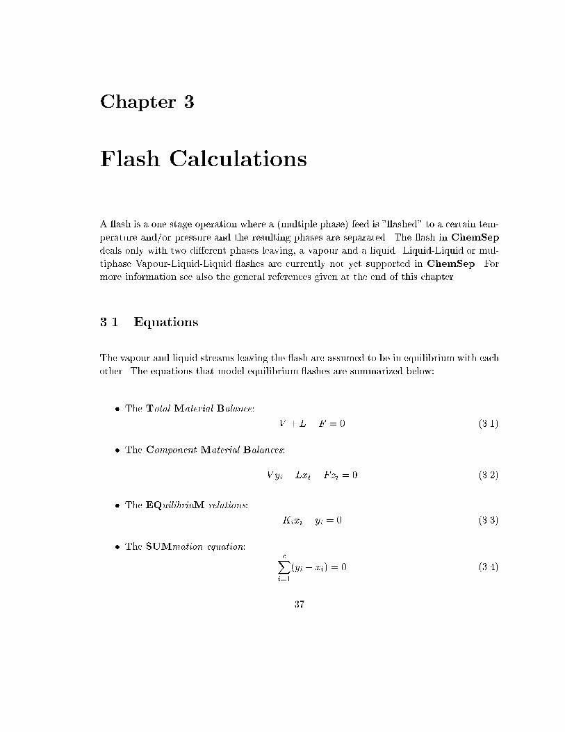
Chapter 3
Flash Calculations
A ash is a one stage operation where a (multiple phase) feed is " ashed" to a certain tem-
perature and/or pressure and the resulting phases are separated. The ash in ChemSep
deals only with two di�erent phases leaving, a vapour and a liquid. Liquid-Liquid or mul-
tiphase Vapour-Liquid-Liquid ashes are currently not yet supported in ChemSep. For
more information see also the general references given at the end of this chapter.
3.1 Equations
The vapour and liquid streams leaving the ash are assumed to be in equilibrium with each
other. The equations that model equilibrium ashes are summarized below:
� The Total Material Balance:
V + L� F = 0 (3.1)
� The Component Material Balances:
V yi + Lxi � Fzi = 0 (3.2)
� The EQuilibriuM relations:
Kixi � yi = 0 (3.3)
� The SUMmation equation:cX
i=1
(yi � xi) = 0 (3.4)
37

p
� The Heat (or entHalpy) balance:
V HV + LHL � FHF +Q = 0 (3.5)
where F is the molar feedrate with component mole fractions zi. V and L are the leaving
vapour and liquid ows with mole fractions yi and xi, respectively. Equilibrium ratios Ki
and enthalpiesH are computed from property models as discussed in chapter 2. Q is de�ned
as the heat added to the feed before the ash. If we count the equations listed, we will �nd
that there are 2c + 3 equations, where c is the number of components. As ash variables
we have (depending on the type of ash):
� c vapour mole fractions, yi;
� c liquid mole fractions, xi;
� vapour owrate, V ;
� liquid owrate, L;
� temperature, T ;
� pressure, p; and
� heat duty, Q.
Since we have 2c + 3 equations, two of the 2c + 5 variables above need not be speci�ed.
ChemSep allows the following nine ash speci�cations:
PT: pressure and temperature
PV: pressure and vapour ow
PL: pressure and liquid ow
PQ: pressure and heat duty
TV: temperature and vapour ow
TL: temperature and liquid ow
TQ: temperature and heat duty
VQ: vapour ow and heat duty
LQ: liquid ow and heat duty
q
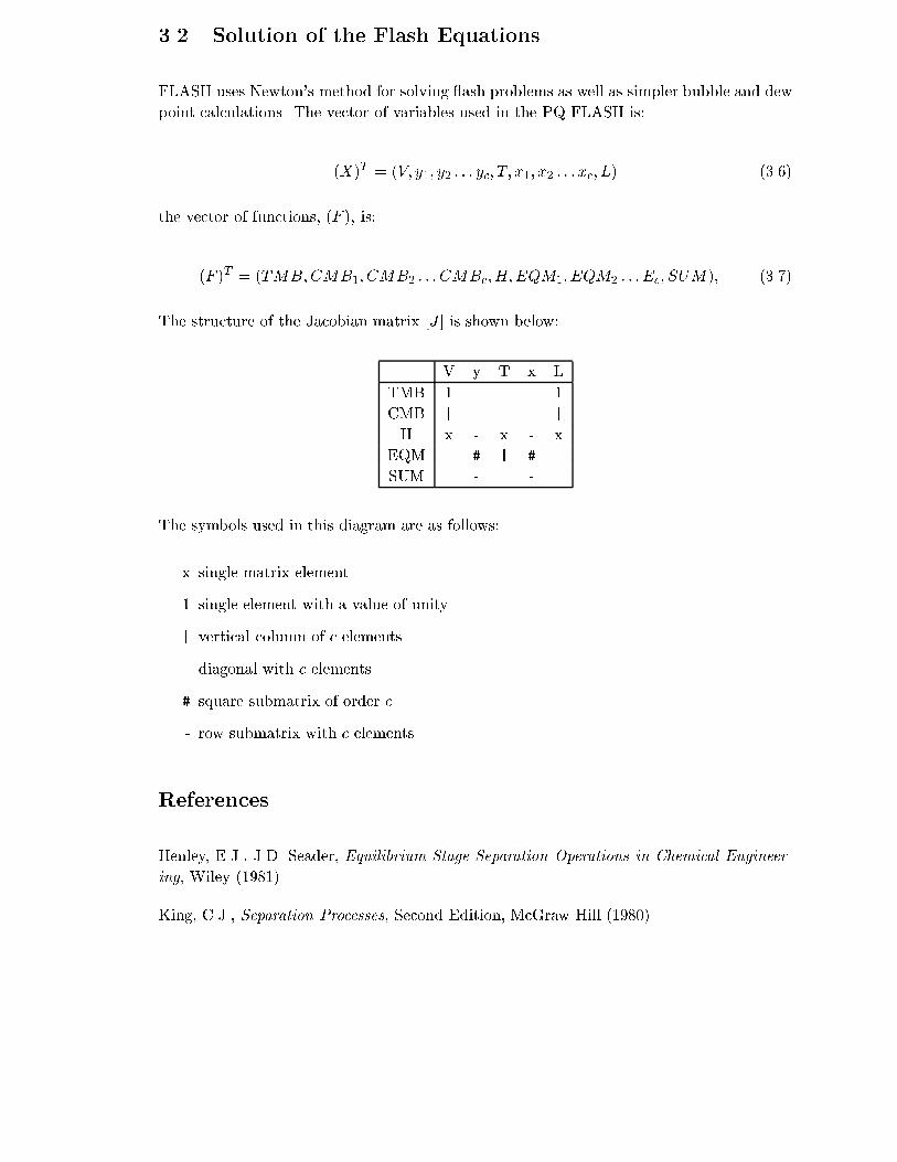
3.2 Solution of the Flash Equations
FLASH uses Newton's method for solving ash problems as well as simpler bubble and dew
point calculations. The vector of variables used in the PQ-FLASH is:
(X)T = (V; y1; y2 : : : yc; T; x1; x2 : : : xc; L) (3.6)
the vector of functions, (F ), is:
(F )T = (TMB;CMB1; CMB2 : : : CMBc;H;EQM1; EQM2 : : : Ec; SUM); (3.7)
The structure of the Jacobian matrix [J ] is shown below:
V y T x L
TMB 1 1
CMB | \ \ |
H x - x - x
EQM # | #
SUM - -
The symbols used in this diagram are as follows:
x single matrix element
1 single element with a value of unity
| vertical column of c elements
\ diagonal with c elements
# square submatrix of order c
- row submatrix with c elements
References
Henley, E.J., J.D. Seader, Equilibrium-Stage Separation Operations in Chemical Engineer-
ing, Wiley (1981).
King, C.J., Separation Processes, Second Edition, McGraw Hill (1980).

p
Chapter 4
Equilibrium Columns
This chapter describes the equilibrium stage model for column operations such as distilla-
tion, absorption and extraction. The equations that ChemSep solves are discussed as well
as other issues.
4.1 Introduction
Multicomponent separation processes like distillation, absorption and extraction have been
modelled using the equilibrium stage concept for a century. The equilibrium stage model
was �rst used by Sorel in 1893 to describe the recti�cation of alcohol. Since that time
it has been applied with ever increasing frequency to all manner of separation processes:
distillation (including recti�cation, stripping, simple (single feed, two product columns),
complex (multiple feed, multiple product columns), extractive, azeotropic and petroleum
re�nery distillation), absorption, stripping, liquid-liquid and supercritical extraction.
The equations that model equilibrium stages are called the MESH equations. The MESH
equations for the interior stages of a column together with equations for the reboiler and
condenser (if they are needed) are solved together with any speci�cation equations to yield,
for each stage, the vapour mole fractions; the liquid mole fractions; the stage temperature
and the vapour and liquid owrates.
Since the late 1950's, hardly a year has gone by without the publication of at least one (and
usually more than one) new algorithm for solving the equilibrium stage model equations.
One of the incentives for the continued activity has always been (and remains) a desire to
solve problems with which existing methods have trouble. The evolution of algorithms for
solving the MESH equations has been in uenced by, among other things: the availability
(or lack) of su�cient computer storage and power, the development of mathematical tech-
41
p q
niques that can be exploited, the complexity of physical property (K-value and enthalpy)
correlations and the form of the model equations being solved.
It is not completely clear who �rst implemented a simultaneous correction method for solv-
ing multicomponent distillation and absorption problems. As is so often the case, it would
appear that the problem was being tackled by a number of people independently. Simul-
taneous solution of all the MESH equations was suggested as a method of last resort by
Friday and Smith (1964) in a classic paper analysing the reasons why other algorithms fail.
They did not, however, implement such a technique. The two best known and most fre-
quently cited papers are those of Goldstein and Stan�eld (1970) and Naphtali and Sandholm
(1971), the latter providing more details of an application of Newton's method described
by Naphtali at an AIChE meeting in May 1965.
To the best of our knowledge, a method to solve all the MESH equations for all stages
at once using Newton's method was �rst implemented by Whitehouse (1964) (see, also,
Stainthorp and Whitehouse, 1967). Among other things, Whitehouse's code allowed for
speci�cations of purity, T, V, L or Q on any stage. Interlinked systems of columns and
nonideal solutions could be dealt with even though no examples of the latter type were
solved by Whitehouse. Since the pioneering work of Whitehouse, Naphtali and Sandholm
and Goldstein and Stan�eld, many others have employed Newton's method or one of its
relatives to solve the MESH equations.
Simultaneous correction procedures have shown themselves to be generally fast and reli-
able. Extensions to the basic method to include complex column con�gurations, interlinked
columns, nonstandard speci�cations and applications to column design result in only minor
changes in the algorithm. In addition, simultaneous correction procedures can easily incor-
porate stage e�ciencies within the calculations (something that is not always possible with
other algorithms). Developments to about 1980 have been described in a number of text-
books (see, for example, Holland, 1963, 1975, 1981; King, 1980; Henley and Seader, 1981)
and a recent review by Wang and Wang (1980). Seader (1985) has written an interesting
history of equilibrium stage simulation.
Seader (1986) lists a number of things to be taken into consideration when designing a
simultaneous correction method; a revised and extended list follows and is discussed in
more detail below.
1. What equations should be used?
2. What variables should be used?
3. How should the equations be ordered?
4. How should the variables be ordered?
5. How should the linearized equations be solved?
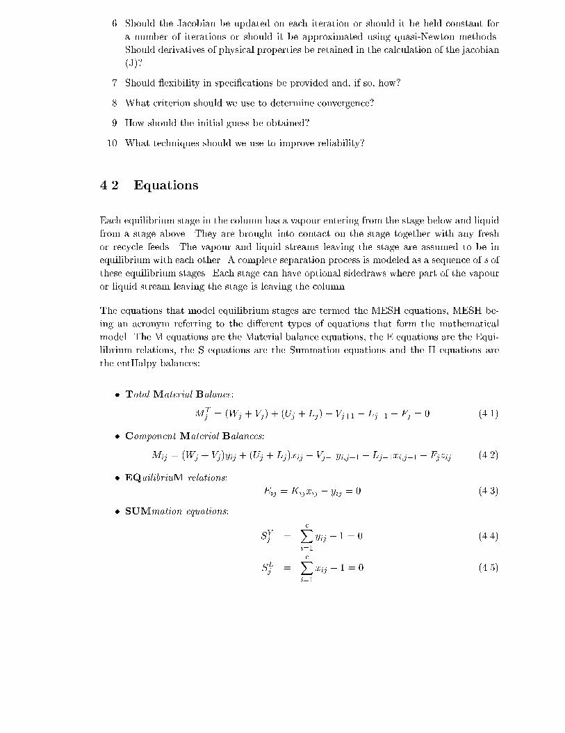
q
6. Should the Jacobian be updated on each iteration or should it be held constant for
a number of iterations or should it be approximated using quasi-Newton methods.
Should derivatives of physical properties be retained in the calculation of the jacobian
(J)?
7. Should exibility in speci�cations be provided and, if so, how?
8. What criterion should we use to determine convergence?
9. How should the initial guess be obtained?
10. What techniques should we use to improve reliability?
4.2 Equations
Each equilibrium stage in the column has a vapour entering from the stage below and liquid
from a stage above. They are brought into contact on the stage together with any fresh
or recycle feeds. The vapour and liquid streams leaving the stage are assumed to be in
equilibrium with each other. A complete separation process is modeled as a sequence of s of
these equilibrium stages. Each stage can have optional sidedraws where part of the vapour
or liquid stream leaving the stage is leaving the column.
The equations that model equilibrium stages are termed the MESH equations, MESH be-
ing an acronym referring to the di�erent types of equations that form the mathematical
model. The M equations are the Material balance equations, the E equations are the Equi-
librium relations, the S equations are the Summation equations and the H equations are
the entHalpy balances:
� Total Material Balance:
MT
j = (Wj + Vj) + (Uj + Lj)� Vj+1 � Lj�1 � Fj = 0 (4.1)
� Component Material Balances:
Mij = (Wj + Vj)yij + (Uj + Lj)xij � Vj+1yi;j+1 � Lj�1xi;j�1 � Fjzij (4.2)
� EQuilibriuM relations:
Eij = Kijxij � yij = 0 (4.3)
� SUMmation equations:
SVj =cX
i=1
yij � 1 = 0 (4.4)
SLj =cX
i=1
xij � 1 = 0 (4.5)

p q
� Heat balance:
Hj = (Wj + Vj)HV
j + (Uj +Lj)HL
j � Vj+1HV
j+1 �Lj�1HL
j�1� FjHF
j +Qj = 0 (4.6)
where we have vapour and liquid leaving ows from stage j, Vj and Lj, with mole fractions
yij and xij , vapour and liquid sidedraws, Wj and Uj , Feeds Fj with mole fractions zij ,
equilibrium K-values Kij , enthalpies Hj, and stage heat duty Qj .
If we count the equations listed, we will �nd that there are 2c + 4 equations per stage.
However, only 2c + 3 of these equations are independent. These independent equations
are generally taken to be the c component mass balance equations, the c equilibrium rela-
tions, the enthalpy balance and two more equations. These two equations can be the two
summation equations or the total mass balance and one of the summation equations (or
an equivalent form). The 2c+ 3 unknown variables determined by the equations are the c
vapour mole fractions, y; the c liquid mole fractions, x; the stage temperature, T and the
vapour and liquid owrates, V and L. For a column of s stages, we must solve s(2c + 3)
equations. The table below shows how we may easily end up having to solve hundreds or
even thousands of equations.
c s s(2c+ 3)
2 10 70
3 20 180
5 50 650
10 30 690
40 100 8300
The �rst entry in this table corresponds to a simple binary problem that could easily be
solved graphically. The second and third are fairly typical of the size of problem encoun-
tered in azeotropic and extractive distillation processes. The last two entries are typical of
problems encountered in simulating hydrocarbon and petroleum mixture separation opera-
tions.
4.3 Condenser and Reboiler
The MESH equations can be applied as written to any of the interior stages of a column.
In addition to these stages, the reboiler and condenser (if they are included) for the column
must be considered. The MESH equations shown above may be used to model these stages
exactly as you would any other stage in the column. For these special stages it is common
to use some speci�cation equation instead of the enthalpy balance. Typical speci�cations
include:

q g
1. the owrate of the distillate/bottoms product stream,
2. the mole fraction of a given component in either the distillate or bottoms product
stream,
3. a component ow rate in either the distillate or bottoms product stream,
4. a re ux/reboil ratio or rate,
5. the temperature of the condenser or reboiler,
6. a heat duty to the condenser or reboiler.
ChemSep includes all of these speci�cations as well as a few others that have not been
listed.
In the case of a total condenser, the vapour phase compositions used in the calculation of the
equilibrium relations and the summation equations are those that would be in equilibrium
with the liquid stream that actually exists. That is for the total condenser, the vapour
composition used in the equilibrium relations is the vapour composition determined during
a bubble point calculation based on the actual pressure and liquid compositions found in
the condenser. At the same time, these compositions are not used in the component mass
balances since there is no vapour stream from a total condenser.
4.4 "Nonequilibrium" Stages
In actual operation the trays of a distillation column rarely, if ever, operate at equilibrium
despite attempts to approach this condition by proper design and choice of operating condi-
tions. The degree of separation is, in fact, determined as much by mass and energy transfer
between the phases being contacted on a tray or within sections of a packed column as it is
by thermodynamic equilibrium considerations. The usual way of dealing with departures
from equilibrium in multistage towers is through the use of stage and/or overall e�ciencies.
The Murphree stage e�ciency is most often used in separation process calculations because
it is easily combined with the equilibrium relations:
Eij = EMV
j Kijxij � yij � (1�EMV
j )yi;j+1 = 0 (4.7)
where EMVj
is the Murphree vapour e�ciency for stage j. If the e�ciency is unity we obtain
the original equilibrium relation from above. The Murphree e�ciency must be speci�ed for
all stages except the condenser and reboiler which are assumed to operate at equilibrium.

p q
4.5 Solution of the MESH Equations
Almost every one of the many numerical methods that have been devised for solving systems
of nonlinear equations has been used to solve the MESH equations. However, as mentioned
earlier, ChemSep uses mostly the Newton's method to solve the nonlinear algebraic MESH
equations. Here we will discuss how ChemSep uses the Newton's method.
4.5.1 How to Order the Equations and Variables?
Separation problems in ChemSep result in stages with each a set of various types of
equations. There are basically two ways to group the equations and variables: by type or by
stage. Grouping the equations and variables by stage is preferred for problems with more
stages than components (practically all distillation and many absorption and extraction
problems) while grouping by type is preferred for systems with more components than
stages (some gas absorption problems). ChemSep employs a by-stage grouping of the
equations and variables. We de�ne a vector of variables for the j-th stage as:
(Xj)T = (Vj ; y1j ; y2j : : : ycj; x1j ; x2j : : : xcj; Lj) (4.8)
and a vector of functions for the j-th stage (Fj):
(Fj)T = (MT
j ;M1j ;M2j : : :Mcj;Hj ; E1j ; E2j : : : Ecj; SL�Vj
) (4.9)
where
SL�V =cX
i=1
(xij � yij) = 0 (4.10)
If the equations and variables are grouped by stage we have
(F )T = ((F1)T ; (F2)
T : : : (Fs)T ) (4.11)
(X)T = ((X1)T ; (X2)
T : : : (Xs)T ) (4.12)

q
4.5.2 The Jacobian
To evaluate the Jacobian matrix, one must obtain the partial derivative of each function
with respect to every variable. Part of the appeal of the grouping by stage approach is that
for single columns at least the Jacobian matrix is block tridiagonal in structure:
[B1] [C1]
[A2] [B2] [C2]
[A3] [B3] [C3]
. . .
. . .
[Am� 1] [Bm� 1] [Cm� 1]
[Am] [Bm]
in which each entry [A], [B], [C] is a matrix in its own right. The [A] submatrices contain
partial derivatives of the equations for the j-th stage with respect to the variables for stage
j � 1. The [B] submatrices contain partial derivatives of the equations for the j-th stage
with respect to the variables for the j-th stage. Finally, the [C] submatrices contain partial
derivatives of the equations for the j-th stage with respect to the variables for stage j + 1.
The structure of the submatrices [A], [B] and [C] is shown below.
[A] [B] [C]
V y T x L V y T x L V y T x L
TMB 1 1 1 1
CMB \ | | \ \ | | \
H x - x x - x - x x - x
EQM # | # \
SUM - -
The symbols used in these diagrams are as follows:
x single matrix element
1 single element with a value of unity
| vertical column of c elements
\ diagonal with c elements
# square submatrix of order c
- row submatrix with c elements

p q
The elements of [B] include partial derivatives of K-values with respect to temperature
and composition. Since it is rather a painful experience to di�erentiate, for example, the
UNIQUAC equations with respect to temperature and composition, in some SC codes
this di�erentiation is done numerically. This can be an extremely time consuming step.
However, neglect of these derivatives is not recommended unless one is dealing with nearly
ideal solutions, since, to do so, will almost certainly lead to an increase in the required
number of iterations or even to failure.
Almost all of the partial derivatives needed in ChemSep are computed from analytical
expressions. The exception is the temperature derivatives of the excess enthalpy which
requires a second di�erentiation with respect to temperature of the activity and fugacity
coe�cient models. Coding just the �rst derivatives was bad enough.
If the column has pumparounds extra matrices will be present which are not on the diagonal
and the use of block tridiagonal methods becomes less straight forward. Similar problems
arise with non-standard speci�cations that are not on the variables of the condenser and re-
boiler. When we solve multiple interlinked columns (currently not supported byChemSep)
a special ordering is required to maintain the diagonal structure of the jacobian. Therefore,
ChemSep now uses a sparse solver to solve the system of equations involved.
4.5.3 How Should the Linearized Equations be Solved?
It is absolutely essential to take account of the sparsity of the Jacobian when solving the
linearized equations; straightforward matrix inversion is totally impractical (and probably
numerically impossible). Linear systems with a block tridiagonal structure may reasonably
e�ciently be solved using a generalized form of the Thomas algorithm. The steps of this
algorithm are given by Henley and Seader (1981).
Still further improvements in the block elimination algorithm for solution of separation pro-
cess problems can be e�ected if we take advantage of the special structure of the submatrices
[A], [B] and [C]. In fact, [A] and [C] are nearly empty. ChemSep uses the sparse matrix
solver NSPIV for solving the sparse linear system e�ectively.
4.5.4 The Initial Guess
In order to obtain convergence, Newton's method requires that reasonable initial estimates
be provided for all s(2c+3) independent variables. ChemSep uses an automatic initializa-
tion procedure where the user does not need to make any guesses. Flow rates are estimated
assuming constant molar ows from stage to stage. If the bottoms ow rate and re ux
ratio are NOT speci�ed and cannot be estimated from the speci�cations that are supplied
then the bottoms ow rate is arbitrarily assigned a value of half the total feed ow and the
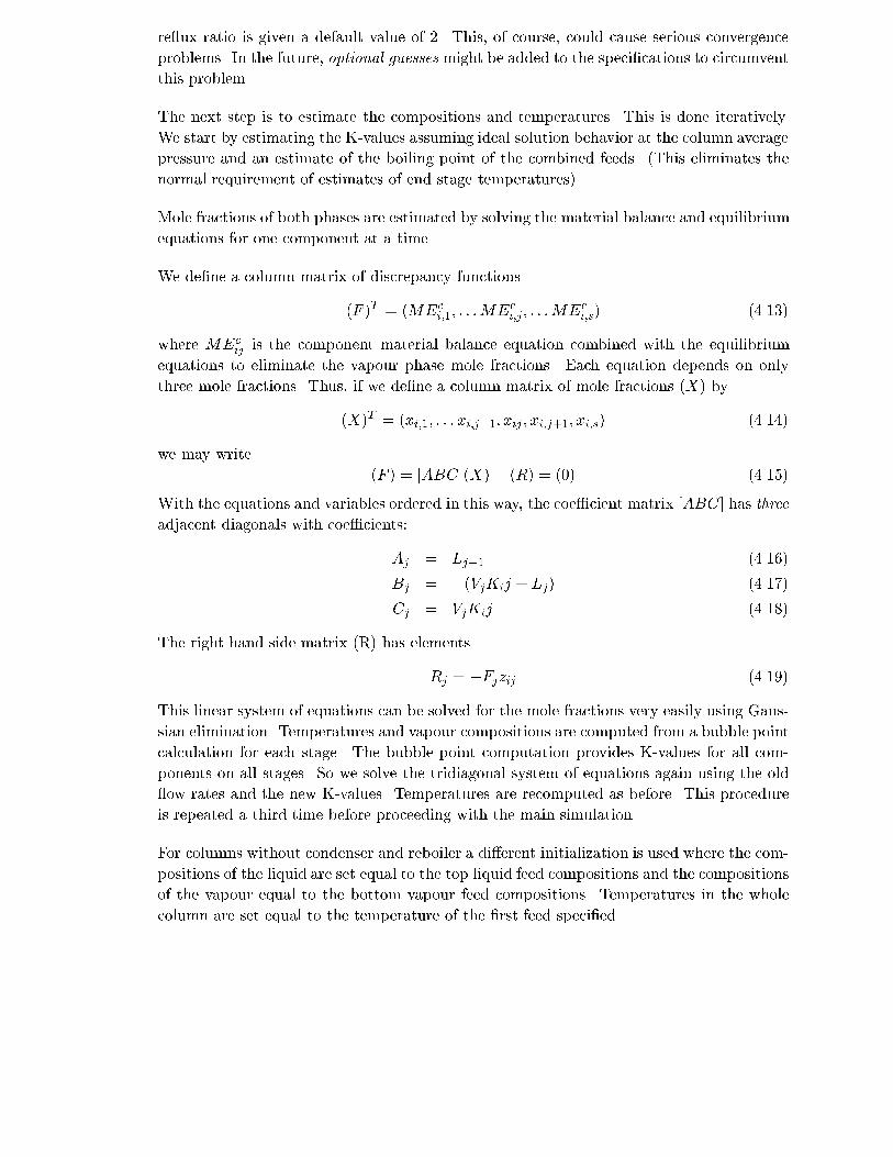
q
re ux ratio is given a default value of 2. This, of course, could cause serious convergence
problems. In the future, optional guesses might be added to the speci�cations to circumvent
this problem.
The next step is to estimate the compositions and temperatures. This is done iteratively.
We start by estimating the K-values assuming ideal solution behavior at the column average
pressure and an estimate of the boiling point of the combined feeds. (This eliminates the
normal requirement of estimates of end stage temperatures).
Mole fractions of both phases are estimated by solving the material balance and equilibrium
equations for one component at a time.
We de�ne a column matrix of discrepancy functions
(F )T = (MEc
i;1; : : : MEc
i;j; : : : MEc
i;s) (4.13)
where MEcijis the component material balance equation combined with the equilibrium
equations to eliminate the vapour phase mole fractions. Each equation depends on only
three mole fractions. Thus, if we de�ne a column matrix of mole fractions (X) by
(X)T = (xi;1; : : : xi;j�1; xij ; xi;j+1; xi;s) (4.14)
we may write
(F ) = [ABC](X)� (R) = (0) (4.15)
With the equations and variables ordered in this way, the coe�cient matrix [ABC] has three
adjacent diagonals with coe�cients:
Aj = Lj�1 (4.16)
Bj = �(VjKij + Lj) (4.17)
Cj = VjKij (4.18)
The right hand side matrix (R) has elements
Rj = �Fjzij (4.19)
This linear system of equations can be solved for the mole fractions very easily using Gaus-
sian elimination. Temperatures and vapour compositions are computed from a bubble point
calculation for each stage. The bubble point computation provides K-values for all com-
ponents on all stages. So we solve the tridiagonal system of equations again using the old
ow rates and the new K-values. Temperatures are recomputed as before. This procedure
is repeated a third time before proceeding with the main simulation.
For columns without condenser and reboiler a di�erent initialization is used where the com-
positions of the liquid are set equal to the top liquid feed compositions and the compositions
of the vapour equal to the bottom vapour feed compositions. Temperatures in the whole
column are set equal to the temperature of the �rst feed speci�ed.

p q
For columns with either a condenser or a reboiler the compositions are initialized to the
overall compositions of all feeds combined, and the temperatures to the bubble point at the
column pressure and the overall feed compositions.
Currently there is no special initialization routine that will handle pumparounds if they
are present. The result is that columns with large pumparound ows will require ow ini-
tialization by the user, or, to repetitively solve the problem using the old results as the
initialization and increasing pumparound ow (see below).
4.5.5 Reliability
SC methods are far more reliable and versatile than most other methods. The same method
will solve distillation, gas absorption and liquid extraction problems. It must be admitted
though, that although the probability that Newton's method will converge from the auto-
matic initial estimates is quite high, there is no guarantee of convergence. The di�culty
of supplying good initial estimates is particularly severe for problems involving strongly
nonideal mixtures, interlinked systems of columns and nonstandard speci�cations.
Several methods have been used to improve the reliability of Newton's method; damping
the Newton step, use of steepest descent (ascent) formulations for some of the iterations,
and combination with relaxation procedures; none of which has proven to be completely
satisfactory. The methods most recently proposed for assisting convergence of Newton's
method are continuation methods.
In default mode, ChemSep does NOT use any of these techniques, other than a check to
make sure that all quantities remain positive. Mole fractions, for example, are not permitted
to take on negative values. The user does have the option of supplying damping factors.
4.5.6 Damping factors
The Newton's method in ChemSep has some extra features that will enhance the conver-
gence to the solution. The Newton's method computes a new solution vector based on the
current Jacobian and function vector. However, the new solution vector might be physically
meaningless, for example if a composition becomes smaller than zero or larger than unity.
Also, the new solution vector might represent a too large a change in stage temperatures
or ows for the method to be stable. To eleviate these problems ChemSep uses damping of
the newton's iteration changes. Temperature changes are limited to a maximum (default
to 10 K) and ow changes up to a maximum fraction of the old ows (default set to 0.5).
The compositions require a special type of damping. If a composition is becoming negative
or larger than unity, the change is limited to half the distance to the extreme. Also, if a
damping factor is speci�ed, the maximum change in composition equals the factor (the de-

q
fault factor is 1 allowing a change over the whole mol fraction range). This type of damping
has turned out to be very e�ective. The damping factors can be found under the Options
- Solve options menu.
If for some reason your column simulation does not converge, changing the damping factors
might help. If you know the iteration history (by either limiting the number of iterations
or by printing out the intermediate answers. Both can be done in the Options - Solve
options menu) you can adapt the factors so the column simulation might converge. Note
that convergence is mostly slower when you start to apply extra damping by making the
factors smaller, the Newton method looses its e�ectiveness when damped. Nor does damping
guarantee convergence.
4.5.7 User Initialization
For di�cult problems it might be necessary for the user to provide initial temperature,
pressure, or ow pro�les. In case the stage temperatures or pressures are not calculated
user initialization is a way to de�ne these pro�les.
The user can specify either temperature or ow pro�les, or both. The only requirement is
that values for the �rst and last stages are provided. Missing temperatures on intermediate
stages are computed by linear interpolation, missing ows are computed on a constant ow
from stage to stage basis. Therefore, it is better to specify the ows of the �rst and last
two stages in case a condenser and reboiler are present. Composition pro�les are computed
through the method described above, however, temperatures are not computed using the
bubble point calculations. If both user speci�ed temperature and ow pro�les are incomplete
ChemSep switches to the automatic initialization method.
4.5.8 Initialization with Old Results
In some cases it might prove advantageous to use the converged results of a previous run
as the initial guess for a new problem (for example, when bottoms owrate and re ux rate
are not speci�ed and cannot be estimated, and the automatic initialization always uses a
re ux ratio of 2). This is a very straight forward way of specifying the initial guess as long
as the number of components remains the same. Care must be taken when feed or product
speci�cations or locations are changed. The results are interpolated if the number of stages
is changed.
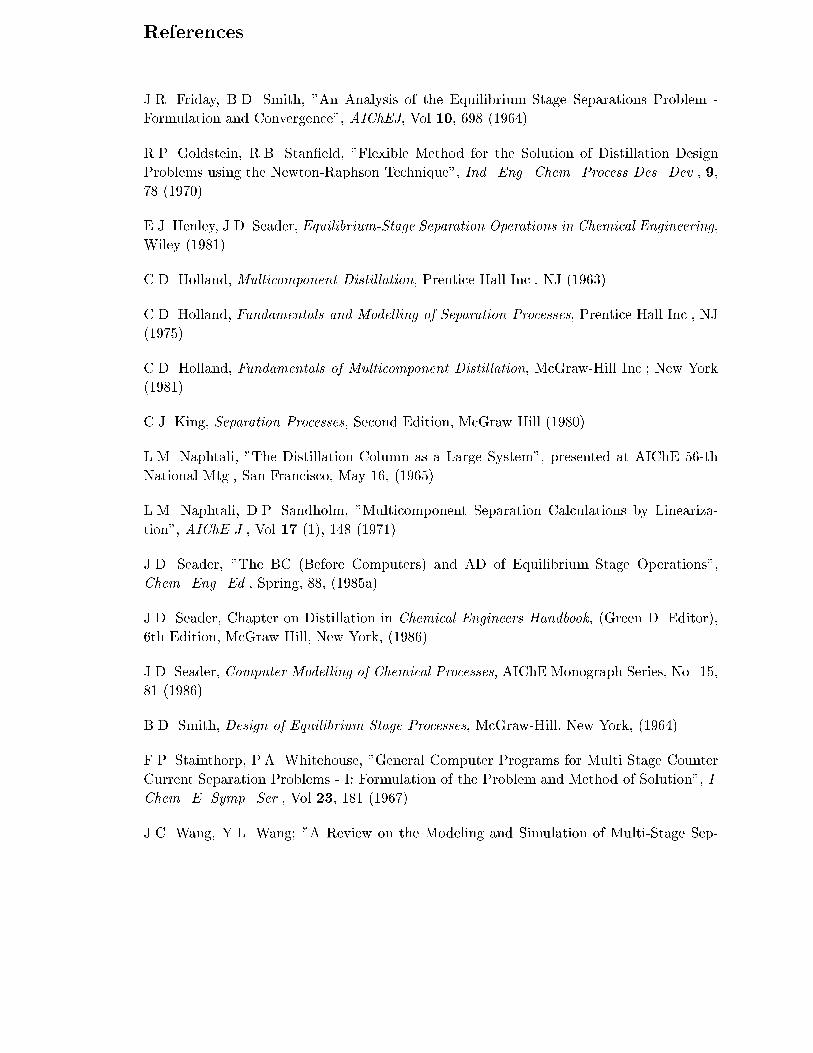
p q
References
J.R. Friday, B.D. Smith, "An Analysis of the Equilibrium Stage Separations Problem -
Formulation and Convergence", AIChEJ, Vol 10, 698 (1964).
R.P. Goldstein, R.B. Stan�eld, "Flexible Method for the Solution of Distillation Design
Problems using the Newton-Raphson Technique", Ind. Eng. Chem. Process Des. Dev., 9,
78 (1970).
E.J. Henley, J.D. Seader, Equilibrium-Stage Separation Operations in Chemical Engineering,
Wiley (1981).
C.D. Holland, Multicomponent Distillation, Prentice Hall Inc., NJ (1963).
C.D. Holland, Fundamentals and Modelling of Separation Processes, Prentice Hall Inc., NJ
(1975).
C.D. Holland, Fundamentals of Multicomponent Distillation, McGraw-Hill Inc.; New York
(1981).
C.J. King, Separation Processes, Second Edition, McGraw Hill (1980).
L.M. Naphtali, "The Distillation Column as a Large System", presented at AIChE 56-th
National Mtg., San Francisco, May 16, (1965).
L.M. Naphtali, D.P. Sandholm, "Multicomponent Separation Calculations by Lineariza-
tion", AIChE J., Vol 17 (1), 148 (1971).
J.D. Seader, "The BC (Before Computers) and AD of Equilibrium Stage Operations",
Chem. Eng. Ed., Spring, 88, (1985a).
J.D. Seader, Chapter on Distillation in Chemical Engineers Handbook, (Green D. Editor),
6th Edition, McGraw Hill, New York, (1986)
J.D. Seader, Computer Modelling of Chemical Processes, AIChE Monograph Series, No. 15,
81 (1986).
B.D. Smith, Design of Equilibrium Stage Processes, McGraw-Hill, New York, (1964).
F.P. Stainthorp, P.A. Whitehouse, "General Computer Programs for Multi Stage Counter
Current Separation Problems - I: Formulation of the Problem and Method of Solution", I.
Chem. E. Symp. Ser., Vol 23, 181 (1967).
J.C. Wang, Y.L. Wang; "A Review on the Modeling and Simulation of Multi-Stage Sep-

aration Processes" in Foundations of Computer-Aided Chemical Process Design, vol. II;
R.S.H. Mah and W.D. Seider, eds.; Engineering Foundation; 121 (1981).
S.M Walas, Phase Equilibria in Chemical Engineering, Butterworth Publishers, (1985).
P.A. Whitehouse, A General Computer Program Solution of Multicomponent Distillation
Problems, Ph.D. Thesis in Chem.Eng., University of Manchester, Institute of Science and
Technology, Manchester, England (1964).

p q
Chapter 5
Nonequilibrium Columns
The nonequilibrium model and the model equations are introduced. Models that describe
the mass transfer, the ow type, pressure drop, entrainment, and weeping are discussed.
The design method which enables the simultaneous design of the the column layout and
column simulation is explained.
5.1 The Nonequilibrium Model
A second generation nonequilibrium model was developed by Taylor and coworkers and is
described in detail by Taylor et al. (1994) and Taylor and Krishna (1993). It can be used
to simulate trayed columns as well as packed columns. Packed columns are simulated with
stages representing a discrete integration over the packed bed. The more stages are used the
better the integration, and the more accurate the results will be (to check if the speci�ed
number of stages in a packed column simulation was su�cient, increase the number of stages
and repeat the column simulation, the results should be similar). A schematic diagram of
a nonequilibrium stage is shown in Figure 5.1. This stage may represent one (or more than
one) tray in a trayed column or a section of packing in a packed column. The vertical wavy
line in the middle of the diagram represents the interface between the two phases which may
be vapor and liquid (distillation), gas and liquid (absorption) or two liquids (extraction).
Figure 5.1 also serves to introduce the notation used in writing down the equations that
model the behavior of this nonequilibrium stage. The ow rates of vapor and liquid phases
leaving the j-th stage are denoted by Vj and Lj respectively. The mole fractions in these
streams are yij and xij. TheNij are the molar uxes of species i on stage j. When multiplied
by the area available for interphase mass transfer we obtain the rates of interphase mass
transfer. The temperatures of the vapor and liquid phases are not assumed to be equal and
we must allow for heat transfer as well as mass transfer across the interface.
55

p q
Lj-1
xi,j-1
Hj-1
Tj-1
L
yi,j
Hj
Tj
V
Vj
vaporside draw
Lj
xi,j
Hj
Tj
L yi,j+1
Hj+1
Tj+1
V
Vj+1
liquidside draw
Qj
fi,j
Hj
Qj
L V
Stage j
N
E
L V
V
V
fi,j
Hj
L
L
L
V
Figure 5.1: Schematic diagram of a nonequilibrium stage (after Taylor and Krishna, 1993).

q
If Figure 5.1 represents a single tray then the term �Ljis the fractional liquid entrainment
de�ned as the ratio of the moles of liquid entrained in the vapor phase in stage j to the
moles of down owing liquid from stage j. Similarly, �Vjis the ratio of vapor entrained in
the liquid leaving stage j (carried down to the tray below under the downcomer) to the
interstage vapor ow. For packed columns, this term represents axial dispersion. Weeping
in tray columns may be accounted for with a similar term.
The component material balance equations for each phase may be written as follows:
MV
ij � (1 + rVj + �Vj )Vjyij � Vj+1yi;j+1 � �Vj�1Vj�1yi;j�1 � fVij �nX
�=1
GV
ij� +Nij
= 0 i = 1; 2; : : : ; c (5.1)
ML
ij � (1 + rLj + �Lj )Ljxij � Lj�1xi;j�1 � �Lj+1Lj+1xi;j+1 � fLij �nX
�=1
GL
ij� �Nij
= 0 i = 1; 2; : : : ; c (5.2)
where Gij� is the interlinked ow rate for component i from stage � to stage j, and n is the
number of total stages (trays or sections of packing). The last terms in Equations (5.1) and
(5.2) are the mass transfer rates (in kmol=s), where mass transfer from the \V" phase to
the \L" phase is de�ned as positive. At the V/L interface we have continuity of mass and,
thus, the mass transfer rates in both phases must be equal.
The total material balances for the two phases are obtained by summing Equations (5.1)
and (5.2) over the component index i.
MV
tj� (1 + rVj + �Vj )Vj � Vj+1 � �Vj�1Vj�1 � F V
j �cX
i=1
nX�=1
GV
ij� +Ntj
= 0 (5.3)
ML
tj� (1 + rLj + �Lj )Lj � Lj�1 � �Lj+1Lj+1 � FL
j �cX
i=1
nX�=1
GL
ij� �Ntj
= 0 (5.4)
Fj denotes the total feed ow rate for stage j, Fj =P
c
i=1 fij.
Here total ow rates and mole fractions are used as independent variables and total as well
as component material balances are included in the set of independent model equations. In
the nonequilibrium model of Krishnamurthy and Taylor (1985a) component ow rates were
treated as variables.
The nonequilibrium model uses two sets of rate equations for each stage:
RV
ij � Nij �NV
ij = 0 i = 1; 2 : : : ; c� 1 (5.5)
RL
ij � Nij �NL
ij = 0 i = 1; 2 : : : ; c� 1 (5.6)
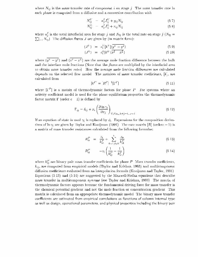
p q
where Nij is the mass transfer rate of component i on stage j. The mass transfer rate in
each phase is computed from a di�usive and a convective contribution with
NV
ij = aIjJV
ij + yijNtj (5.7)
NL
ij = aIjJL
ij + xijNtj (5.8)
where aIjis the total interfacial area for stage j and Ntj is the total rate on stage j (Ntj =P
c
i=1Nij). The di�usion uxes J are given by (in matrix form):
(JV ) = cVt [kV ](yV � yI) (5.9)
(JL) = cLt [kL](xI � xL) (5.10)
where (yV � yI) and (xI � xL) are the average mole fraction di�erence between the bulk
and the interface mole fractions (Note that the uxes are multiplied by the interfacial area
to obtain mass transfer rates). How the average mole fraction di�erences are calculated
depends on the selected ow model. The matrices of mass transfer coe�cients, [k], are
calculated from
[kP ] = [RP ]�1[�P ] (5.11)
where [�P ] is a matrix of thermodynamic factors for phase P . For systems where an
activity coe�cient model is used for the phase equilibrium properties the thermodynamic
factor matrix � (order c� 1) is de�ned by
�ij = �ij + xi
@ ln i
@xj
!T;P;xk;k 6=j=1:::c�1
(5.12)
If an equation of state is used i is replaced by �i. Expressions for the composition deriva-
tives of ln i are given by Taylor and Kooijman (1991). The rate matrix [R] (orderc� 1) is
a matrix of mass transfer resistances calculated from the following formulae:
RP
ii =zi
kPic
+cX
k=1;k 6=i
zk
kPik
(5.13)
RP
ij = �zi
1
kPij
�1
kPic
!(5.14)
where kPijare binary pair mass transfer coe�cients for phase P . Mass transfer coe�cients,
kij , are computed from empirical models (Taylor and Krishna, 1993) and multicomponent
di�usion coe�cients evaluated from an interpolation formula (Kooijman and Taylor, 1991).
Equations (5.13) and (5.14) are suggested by the Maxwell-Stefan equations that describe
mass transfer in multicomponent systems (see Taylor and Krishna, 1993). The matrix of
thermodynamic factors appears because the fundamental driving force for mass transfer is
the chemical potential gradient and not the mole fraction or concentration gradient. This
matrix is calculated from an appropriate thermodynamic model. The binary mass transfer
coe�cients are estimated from empirical correlations as functions of column internal type
as well as design, operational parameters, and physical properties including the binary pair
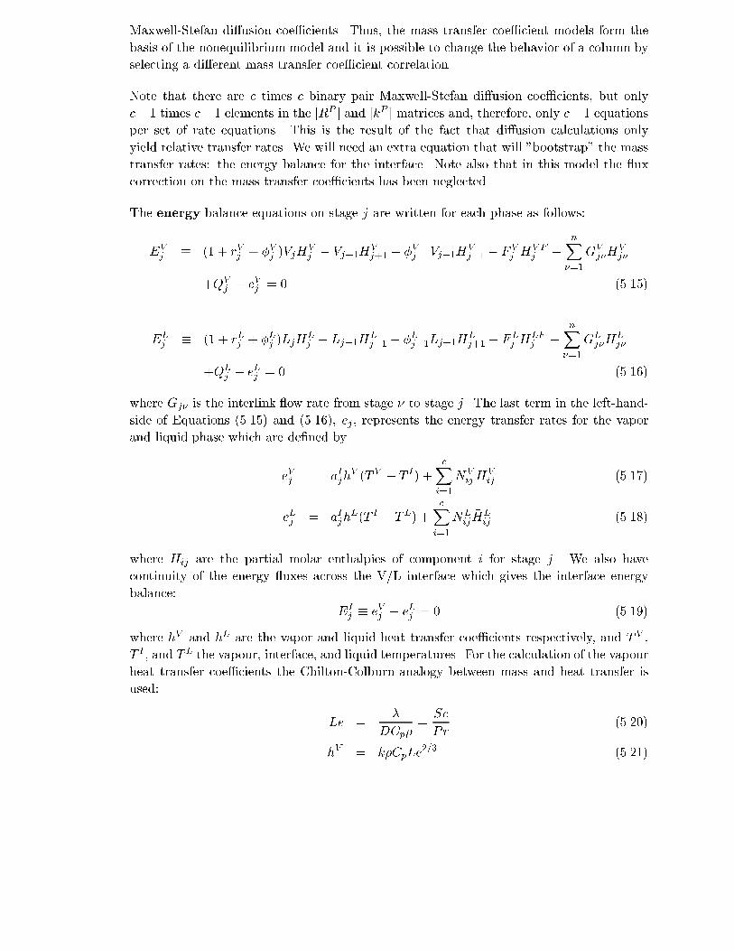
q
Maxwell-Stefan di�usion coe�cients. Thus, the mass transfer coe�cient models form the
basis of the nonequilibrium model and it is possible to change the behavior of a column by
selecting a di�erent mass transfer coe�cient correlation.
Note that there are c times c binary pair Maxwell-Stefan di�usion coe�cients, but only
c� 1 times c� 1 elements in the [RP ] and [kP ] matrices and, therefore, only c� 1 equations
per set of rate equations. This is the result of the fact that di�usion calculations only
yield relative transfer rates. We will need an extra equation that will "bootstrap" the mass
transfer rates: the energy balance for the interface. Note also that in this model the ux
correction on the mass transfer coe�cients has been neglected.
The energy balance equations on stage j are written for each phase as follows:
EV
j � (1 + rVj + �Vj )VjHV
j � Vj+1HV
j+1 � �Vj�1Vj�1HV
j�1 � F V
j HV F
j �nX
�=1
GV
j�HV
j�
+QV
j + eVj = 0 (5.15)
EL
j � (1 + rLj + �Lj )LjHL
j � Lj�1HL
j�1 � �Lj+1Lj+1HL
j+1 � FL
j HLF
j �nX
�=1
GL
j�HL
j�
+QL
j � eLj = 0 (5.16)
where Gj� is the interlink ow rate from stage � to stage j. The last term in the left-hand-
side of Equations (5.15) and (5.16), ej , represents the energy transfer rates for the vapor
and liquid phase which are de�ned by
eVj = aIjhV (T V � T I) +
cXi=1
NV
ij�HV
ij (5.17)
eLj = aIjhL(T I � TL) +
cXi=1
NL
ij�HL
ij (5.18)
where �Hij are the partial molar enthalpies of component i for stage j. We also have
continuity of the energy uxes across the V/L interface which gives the interface energy
balance:
EI
j � eVj � eLj = 0 (5.19)
where hV and hL are the vapor and liquid heat transfer coe�cients respectively, and T V ,
T I , and TL the vapour, interface, and liquid temperatures. For the calculation of the vapour
heat transfer coe�cients the Chilton-Colburn analogy between mass and heat transfer is
used:
Le =�
DCp�=Sc
Pr(5.20)
hV = k�CpLe2=3 (5.21)

p q
For the calculation of the liquid heat transfer coe�cients a penetration model is used:
hL = k�CppLe (5.22)
where k is the average mass transfer coe�cient and D the average di�usion coe�cient.
In the nonequilibrium model of Krishnamurthy and Taylor (1985a) the pressure was taken
to be speci�ed on all stages. However, column pressure drop is a function of tray (or
packing) type and design and column operating conditions, information that is required for
or available during the solution of the nonequilibrium model equations. It was, therefore,
quite straightforward to add an hydraulic equation to the set of independent equations
for each stage and to make the pressure of each stage (tray or packed section) an unknown
variable. The stage is assumed to be at mechanical equilibrium so pVj= pL
j= pj.
In the second generation model, the pressure of the top tray (or top of the packing) is
speci�ed along with the pressure of any condenser. The pressure of trays (or packed sections)
below the topmost are calculated from the pressure of the stage above and the pressure drop
on that tray (or over that packed section). If the column has a condenser (which is numbered
as stage 1 here) the hydraulic equations are expressed as follows:
P1 � pc � p1 = 0 (5.23)
P2 � pspec � p2 = 0 (5.24)
Pj � pj � pj�1 � (�pj�1) = 0 j = 3; 4; : : : ; n (5.25)
where pc is the speci�ed condenser pressure, pspec is the speci�ed pressure of the tray or
section of packing at the top of the column, and �pj�1 is the pressure drop per tray or
section of packing from section/stage j � 1 to section/stage j. If the top stage is not a
condenser, the hydraulic equations are expressed as
P1 � pspec � p1 = 0 (5.26)
Pj � pj � pj�1 � (�pj�1) = 0 j = 2; 3; : : : ; n (5.27)
In general we may consider the pressure drop to be a function of the internal ows, the uid
densities, and equipment design parameters.
�pj�1 = f(Vj�1; Lj�1; �V
j�1; �L
j�1;Design) (5.28)
The pressure drop term, �pj�1, is calculated from liquid heights on the tray (from various
correlations, see Lockett, 1986, and Kister, 1992) or speci�c pressure drop correlations for
packings (see the section below on pressur drop models).
For bubble cap trays the procedures described by Bolles (1963) can be adapted for computer
based calculation. Kister (1992) also covers methods available for estimating the pressure

q
Table 5.1: Nonequilibrium model equations type and number
Equation Number
Material balances 2c+ 2
Energy balances 3
transfer Rate equations 2c� 2
Summations equations 2
Hydraulic equation 1
interface eQuilibrium relations c
Total MERSHQ 5c+ 6
drop in dumped packed columns. The pressure drop in structured packed columns may
estimated using the method of Bravo et al. (1986).
Phase equilibrium is assumed to exist only at the interface with the mole fractions in both
phases related by:
QI
ij � KijxI
ij � yIij = 0 i = 1; 2; : : : ; c (5.29)
where Kij is the equilibrium ratio for component i on stage j. The Kij are evaluated at
the (calculated) temperature, pressure, and mole fractions at the interface.
The mole fractions must sum to unity in each phase:
SVj �cX
i=1
yij � 1 = 0 (5.30)
SLj �cX
i=1
xij � 1 = 0 (5.31)
as well as at the interface:
SV Ij �cX
i=1
yIij � 1 = 0 (5.32)
SLIj �cX
i=1
xIij � 1 = 0 (5.33)
Table 5.1 lists the type and number of equations for the nonequilibrium model. To solve
the model we have 5c + 6 equations and variables, where c is the number of components.
They are solved simultaneously using Newton's method.
Nonequilibrium and equilibrium models require similar speci�cations. Feed ows and their
thermal condition must be speci�ed for both models, as must the column con�guration
(number of stages, feed and sidestream locations etc.). Additional speci�cations that are
the same for both simulation models include the speci�cation of, for example, re ux ratios or
bottom product ow rates if the column is equipped with a condenser and/or a reboiler. The

p q
Table 5.2: Currently supported column internals for the nonequilibrium model
Bubble-cap trays
Sieve trays
Valve trays (including double weight valves)
Dumped packings
Structured packings
Equilibrium stage (with Murphree stage e�ciency)
Rotating Disk Contactor (RDC) compartment (for extraction)
speci�cation of the pressure on each stage is necessary if the pressure drop is not computed;
if it is, only the top stage pressure needs be speci�ed (the pressure of all other stages being
determined from the pressure drop equations that are part of the model described above).
If we solve the nonequilibrium model with Newton's method, we also require initial guesses
for all the variables. ChemSep uses the same automatic initial guess routine for the
nonequilibriummodel as the equilibrium model. The temperatures of the vapour, interface,
and liquid are initialized all equal to the temperature from the automatic guess. Mass and
energy transfer rates are initialized as zero and the interface mole fractions are set equal
to the bulk mole fractions which are also provided by the initial guess. Pressure drops are
initially assumed to be zero.
The nonequilibrium model, in comparison with the equilibrium model, requires the eval-
uation of many more physical properties and of the heat and mass transfer coe�cients.
In addition, a nonequilibrium simulation cannot proceed without some knowledge of the
column type and the internals layout. Tray type and mechanical layout data, for exam-
ple, is needed in order to calculate the mass transfer coe�cients for each tray. For packed
columns the packing type, size and material must be known. Libraries with standard tray
and packing data are available on-line. Table 5.2 lists the currently supported types of
column internals.
To avoid the problem that during the design of a column no column layout is available, the
nonequilibrium column simulator has an optional design mode to automatically assign layout
parameters. The user just needs to select one of the types of internals (for each section in
the column). The design-mode is activated by not specifying the column diameter (leaving
it as a "default" with "*") for a speci�c section. With the design-mode "on" each tray or
stage is automatically adapted during each iteration while keeping the layout within each
section the same.
For the evaluation of the heat and mass transfer coe�cients, pressure drop, and the en-
trainment/weeping ows a nonequilibrium simulation needs the following:
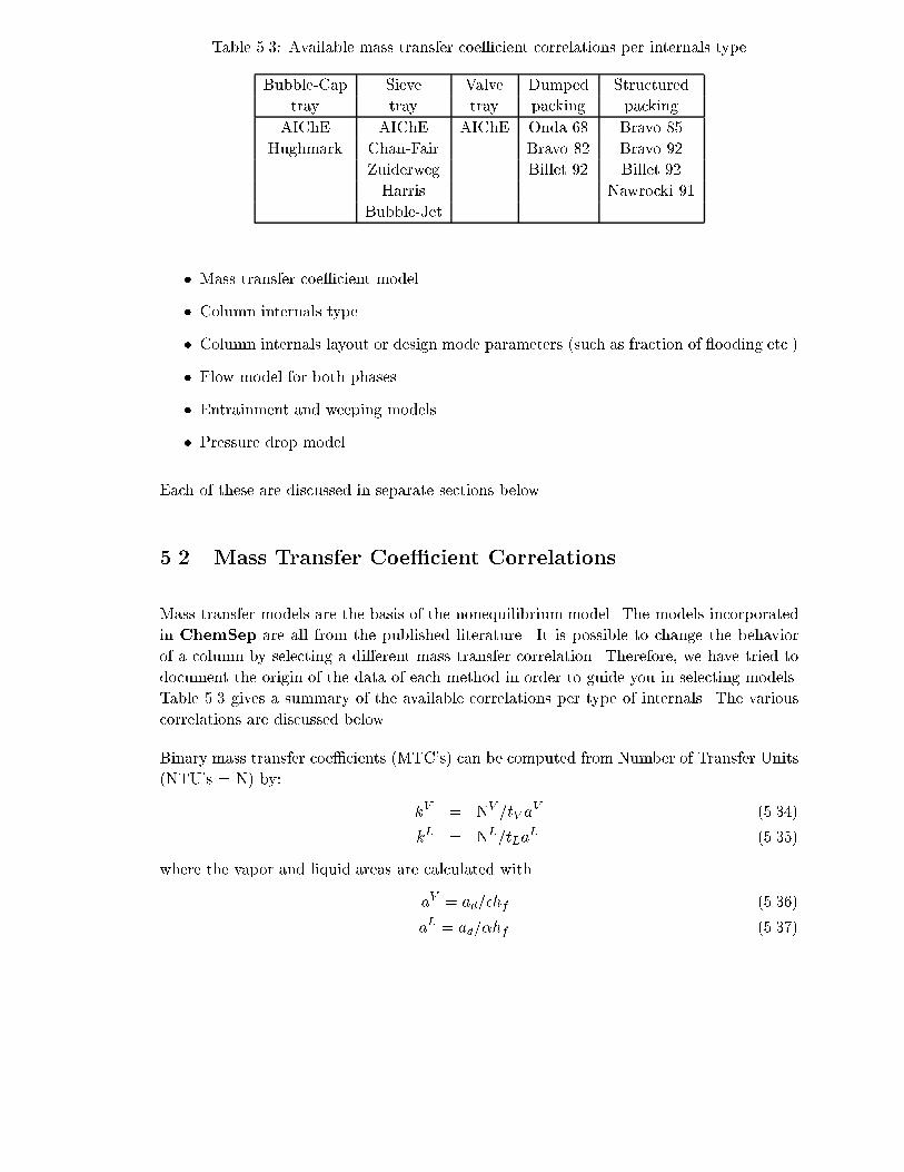
Table 5.3: Available mass transfer coe�cient correlations per internals type
Bubble-Cap Sieve Valve Dumped Structured
tray tray tray packing packing
AIChE AIChE AIChE Onda 68 Bravo 85
Hughmark Chan-Fair Bravo 82 Bravo 92
Zuiderweg Billet 92 Billet 92
Harris Nawrocki 91
Bubble-Jet
� Mass transfer coe�cient model
� Column internals type
� Column internals layout or design mode parameters (such as fraction of ooding etc.)
� Flow model for both phases
� Entrainment and weeping models
� Pressure drop model
Each of these are discussed in separate sections below.
5.2 Mass Transfer Coe�cient Correlations
Mass transfer models are the basis of the nonequilibrium model. The models incorporated
in ChemSep are all from the published literature. It is possible to change the behavior
of a column by selecting a di�erent mass transfer correlation. Therefore, we have tried to
document the origin of the data of each method in order to guide you in selecting models.
Table 5.3 gives a summary of the available correlations per type of internals. The various
correlations are discussed below.
Binary mass transfer coe�cients (MTC's) can be computed from Number of Transfer Units
(NTU's = N) by:
kV = NV =tV aV (5.34)
kL = NL=tLaL (5.35)
where the vapor and liquid areas are calculated with
aV = ad=�hf (5.36)
aL = ad=�hf (5.37)
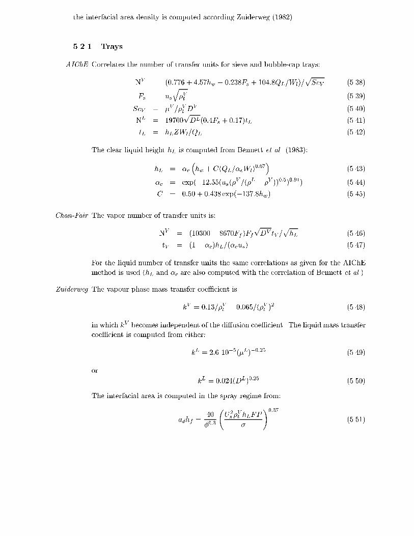
p q
the interfacial area density is computed according Zuiderweg (1982).
5.2.1 Trays
AIChE Correlates the number of transfer units for sieve and bubble-cap trays:
NV = (0:776 + 4:57hw � 0:238Fs + 104:8QL=Wl)=pScV (5.38)
Fs = us
q�Vt (5.39)
ScV = �V =�Vt DV (5.40)
NL = 19700pDL(0:4Fs + 0:17)tL (5.41)
tL = hLZWl=QL (5.42)
The clear liquid height hL is computed from Bennett et al. (1983):
hL = �e
�hw + C(QL=�eWl)
0:67�
(5.43)
�e = exp(�12:55(us(�V =(�L � �V ))0:5)0:91) (5.44)
C = 0:50 + 0:438 exp(�137:8hw) (5.45)
Chan-Fair The vapor number of transfer units is:
NV = (10300 � 8670Ff )FfpDV tV =
phL (5.46)
tV = (1� �e)hL=(�eus) (5.47)
For the liquid number of transfer units the same correlations as given for the AIChE
method is used (hL and �e are also computed with the correlation of Bennett et al.).
Zuiderweg The vapour phase mass transfer coe�cient is
kV = 0:13=�Vt � 0:065=(�Vt )2 (5.48)
in which kV becomes independent of the di�usion coe�cient. The liquid mass transfer
coe�cient is computed from either:
kL = 2:6 10�5(�L)�0:25 (5.49)
or
kL = 0:024(DL)0:25 (5.50)
The interfacial area is computed in the spray regime from:
adhf =40
�0:3
U2s �
Vt hLFP
�
!0:37
(5.51)
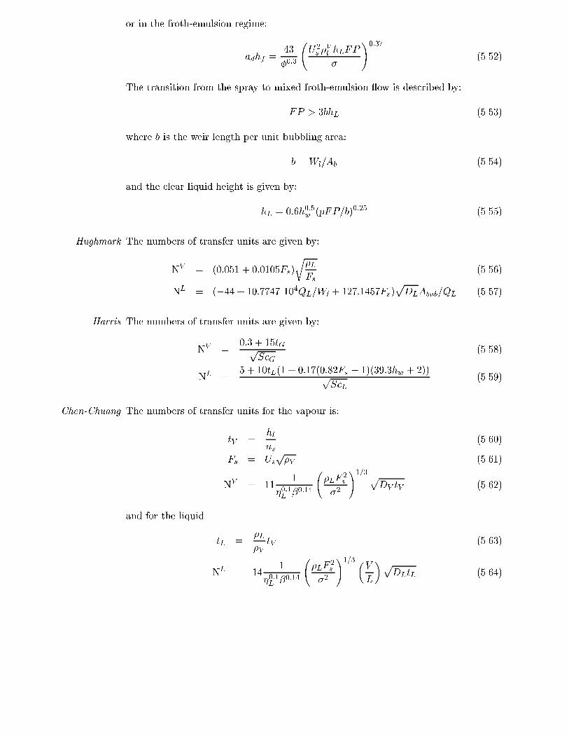
or in the froth-emulsion regime:
adhf =43
�0:3
U2s �
Vt hLFP
�
!0:37
(5.52)
The transition from the spray to mixed froth-emulsion ow is described by:
FP > 3bhL (5.53)
where b is the weir length per unit bubbling area:
b =Wl=Ab (5.54)
and the clear liquid height is given by:
hL = 0:6h0:5w (pFP=b)0:25 (5.55)
Hughmark The numbers of transfer units are given by:
NV = (0:051 + 0:0105Fs)
r�L
Fs(5.56)
NL = (�44 + 10:7747 104QL=Wl + 127:1457Fs)pDLAbub=QL (5.57)
Harris The numbers of transfer units are given by:
NV =0:3 + 15tGp
ScG(5.58)
NL =5 + 10tL(1 + 0:17(0:82Fs � 1)(39:3hw + 2))
pScL
(5.59)
Chen-Chuang The numbers of transfer units for the vapour is:
tV =hl
us(5.60)
Fs = Usp�V (5.61)
NV = 111
�0:1L�0:14
�LF
2s
�2
!1=3pDV tV (5.62)
and for the liquid
tL =�L
�VtV (5.63)
NL = 141
�0:1L�0:14
�LF
2s
�2
!1=3 �V
L
�pDLtL (5.64)
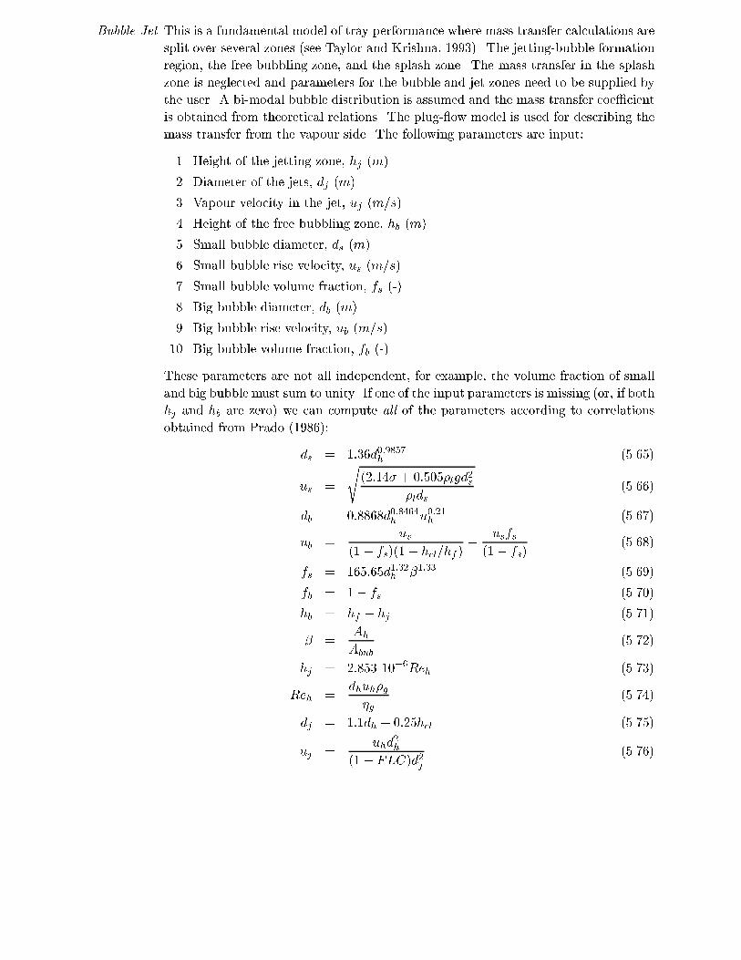
p q
Bubble-Jet This is a fundamental model of tray performance where mass transfer calculations are
split over several zones (see Taylor and Krishna, 1993). The jetting-bubble formation
region, the free bubbling zone, and the splash zone. The mass transfer in the splash
zone is neglected and parameters for the bubble and jet zones need to be supplied by
the user. A bi-modal bubble distribution is assumed and the mass transfer coe�cient
is obtained from theoretical relations. The plug- ow model is used for describing the
mass transfer from the vapour side. The following parameters are input:
1. Height of the jetting zone, hj (m)
2. Diameter of the jets, dj (m)
3. Vapour velocity in the jet, uj (m=s)
4. Height of the free bubbling zone, hb (m)
5. Small bubble diameter, ds (m)
6. Small bubble rise velocity, us (m=s)
7. Small bubble volume fraction, fs (-)
8. Big bubble diameter, db (m)
9. Big bubble rise velocity, ub (m=s)
10. Big bubble volume fraction, fb (-)
These parameters are not all independent, for example, the volume fraction of small
and big bubble must sum to unity. If one of the input parameters is missing (or, if both
hj and hb are zero) we can compute all of the parameters according to correlations
obtained from Prado (1986):
ds = 1:36d0:9857h (5.65)
us =
s(2:14� + 0:505�lgd2s
�lds(5.66)
db = 0:8868d0:8464h u0:21h (5.67)
ub =uv
(1� fs)(1� hcl=hf )�
usfs
(1� fs)(5.68)
fs = 165:65d1:32h �1:33 (5.69)
fb = 1� fs (5.70)
hb = hf � hj (5.71)
� =Ah
Abub
(5.72)
hj = 2:853 10�6Reh (5.73)
Reh =dhuh�g
�g(5.74)
dj = 1:1dh + 0:25hcl (5.75)
uj =uhd
2h
(1� FLC)d2j
(5.76)

where parameters as hf and hcl can be computed by empirical correlations for the
tray (here sieve tray since the correlations were obtained with that particular tray
type). The fraction of inactive holes, FLC, can be set to zero or estimated by
FLC = 1836:97u�1:602h
Q0:524L h0:292w (5.77)
Currently this model is not available in ChemSep.
5.2.2 Random Packings
OTO-68 Onda et al. (1968) [parameters ap, dp, �c] developed correlations of mass transfer
coe�cients for gas absorption, desorption, and vaporization in random packings. The
vapor phase mass transfer coe�cient is obtained from
kV = ARe0:7V Sc0:333V (apDV )(apdp)
�2 (5.78)
where A = 2 if dp < 0:012 and A = 5:23 otherwise. Vapour and liquid velocities are
calculated by
uV = VMV =�VAt (5.79)
uL = LML=�LAt (5.80)
and Reynolds and Schmidt numbers:
ReV =�V uV
(�V ap)(5.81)
ReL =�LuL
(�Lap)(5.82)
ScV =�V
(�Vt DV )
(5.83)
ScL =�L
(�Lt DL)
(5.84)
The liquid phase mass transfer coe�cient is
kL = 0:0051(ReIL)2=3Sc�0:5
L(apdp)
0:4(�Lg=�L)1=3 (5.85)
where ReILis the liquid Reynolds number based on the interfacial area density
ReIL =�LuL
(�Lad)(5.86)
The interfacial area density, ad (m2=m3), is computed from
ad = ap
h1� exp
��1:45(�c=�)0:75Re0:1L Fr�0:05
LWe0:2L
�i(5.87)
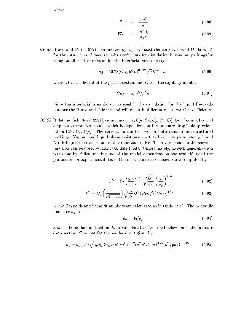
p q
where
FrL =apu
2L
g(5.88)
WeL =�Lu
2L
ap�(5.89)
BF-82 Bravo and Fair (1982) [parameters ap, dp, �c] used the correlations of Onda et al.
for the estimation of mass transfer coe�cients for distillation in random packings by
using an alternative relation for the interfacial area density:
ad = 19:78(CaLReV )0:392
p�H�0:4ap (5.90)
where H is the height of the packed section and Cal is the capillary number
CaL = uL�L=�L� (5.91)
Since the interfacial area density is used in the calculation for the liquid Reynolds
number the Bravo and Fair method will result in di�erent mass transfer coe�cients.
BS-92 Billet and Schultes (1992) [parameters ap, �, Cfl, Ch, Cp, Cv, Cl] describe an advanced
empirical/theoretical model which is dependent on the pressure drop/holdup calcu-
lation (Ch, Cp, Cfl). The correlation can be used for both random and structured
packings. Vapour and liquid phase resistance are �tted each by parameter (Cv and
Cl), bringing the total number of parameters to �ve. There are trends in the parame-
ters that can be observed from tabulated data. Unfortunately, no such generalization
was done by Billet, making use of the model dependent on the availability of the
parameters or experimental data. The mass transfer coe�cients are computed by
kL = Cl
�g�l
�l
�1=6sDL
dh
uL
ap
!1=3
(5.92)
kV = Cv
�1
p�� ht
�ra
dhDV (ReV )
3=4(ScV )1=3 (5.93)
where Reynolds and Schmidt numbers are calculated as in Onda et al.. The hydraulic
diameter dh is
dh = 4�=ap (5.94)
and the liquid holdup fraction, ht, is calculated as described below under the pressure
drop section. The interfacial area density is given by:
ad = ap(1:5=qapdh)(uLdh�
L=�L)�0:2(u2L�Ldh=�)
0:75(u2L=gdh)�0:45 (5.95)

5.2.3 Structured packings
BRF-85 Bravo et al. (1985) [parameters ap, �, B, hc, S, Deq, �] published correlations for
structured packings. This method is based on the assumption that the surface is
completely wetted and that the interfacial area density is equal to the speci�c packing
surface: ad = ap. The Sherwood number for the vapour phase is
ShV = 0:0338Re0:8V Sc0:333V (5.96)
and is de�ned by
ShV =kV deq
DV(5.97)
The equivalent diameter of a channel is given by
deq = Bhc [1=(B + 2S) + 1=2S] (5.98)
where B is the base of the triangle (channel base), S is the corrugation spacing
(channel side), and hc is the height of the triangle (crimp height). The vapour phase
Reynolds number is de�ned by
ReV =deq�
V (uV;eff + uL;eff )
�V(5.99)
The e�ective velocity of vapour through the channel, uV e, is
uV;eff = uV =(� sin �) (5.100)
(uV is the super�cial vapour velocity, � the void fraction, and � the angle of the channel
with respect to the horizontal). The e�ective velocity of the liquid is
uL;eff =3�
2�L
(�L)2g
3�L�
!1=3
(5.101)
where � is the liquid ow rate per unit of perimeter
� = �LuL=P (5.102)
where P is the perimeter per unit cross-sectional area, computed from
P = (4S +B)=Bhc (5.103)
The penetration model is used to predict the liquid phase mass transfer coe�cients
with the exposure time assumed to be the time required for the liquid to ow between
corrugations (a distance equal to the channel side):
tL = S=uL;eff (5.104)
kL = 2
sDL
�tL(5.105)

p q
NXC-91 Nawrocki et al. (1991) [parameter P ] developed a combination of a theoretical model
for the liquid distribution in structured packing and the empirical correlation of Bravo
et al. (1985) for the mass transfer coe�cients. It is capable of predicting the mass
transfer coe�cients in mall-distributed columns. Unfortunately, values of the model
parameter P are unknown for any packing and must be evaluated from experimental
data. Currently this model is not available in ChemSep.
BRF-92 Bravo et al. (1992) [parameters ap, �, S, �, Fse, K2, Ce, dPdzflood] developed a
theoretical model for modern structured packings. Four parameters can be supplied,
however, the authors advise a �xed value for the surface renewal correction (Ce),
normally 0:9. They provide a relation for parameter K2 as well:
K2 = 0:614 + 71:35S (5.106)
The mass transfer calculations are dependent on the pressure drop/holdup calcula-
tions. The e�ective area can be adjusted with the surface enhancement factor Fse,
and the liquid resistance with a correction on the surface renewal following the pene-
tration model (parameter Ce). E�ective velocities are computed with
uL;eff = uL=�ht sin � (5.107)
uG;eff = uV =�(1 � ht) sin � (5.108)
where ht is the fractional liquid holdup (see below at the section on pressure drop
calculation). Reynolds numbers and liquid mass transfer coe�cient is now calculated
as in Bravo et al. (1985) but with
tL = CeS=uL;eff (5.109)
However, the vapour phase mass transfer coe�cient is obtained from
kV = 0:054(DV
S)Re0:8V Sc
1=3V
(5.110)
where the equivalent diameter is replaced with the channel side S and a di�erent
coe�cient is used. The assumption of a completely wetted packing is dropped, the
interfacial area density is given by
ad = FtFseap (5.111)
Ft =29:12(WeLFrL)
0:15S0:359
Re0:2L�0:6(sin �)0:3(1� 0:93 cos )
(5.112)
where cos is equal to 0:9 for � < 0:0453, otherwise it is computed by
cos = 5:211 10�16:835� (5.113)
Note that a di�erent switch point is used than reported by Bravo et al. (1992) to
guarantee continuity in cos .
BS-92 Billet and Schultes (1992) [parameters ap, �, Cfl, Ch, Cp, Cv, Cl] developed a model
for both random and structured packings, see the section on random packings above.

5.3 Flow Models
For the calculation of the di�usion uxes the average mole fraction di�erence between the
bulk and the interface mole fractions were required (see Equations 5.9 and 5.10). How these
average mole fraction di�erences are computed depends on the selected ow model. Here
three ow models are discussed: mixed ow, plug ow, and dispersion ow (which is only
applied to the liquid phase).
5.3.1 Mixed ow
If we assume both phases are present in a completely mixed state, we can use
(yV � yI) = (yV � yI) (5.114)
(xI � xL) = (xI � xL) (5.115)
this keeps the rate equations (relatively) simple and only a function of the mole fractions
leaving the current stage. However, on a tray where the vapour bubbles through a liquid
which ows from one downcomer to the opposite downcomer this model is not accurate.
Indeed, only for very small diameter columns will the mixed ow model give reasonable
results. The mixed model is the most simple ow model and is the easiest to converge. For
packed columns the convergence to the true column pro�les by using increasing number of
stages can be quite slow using the mixed ow model.
5.3.2 Plug ow
In the plug- ow model we assume that the vapour or liquid moves in plug ow (thus, with-
out mixing) through the froth. This complicates the rate equations so much that no exact
solution is possible. The mass transfer actually needs to be integrated over the froth. To
approximate the total mass transfer an average mole fraction di�erence is computed. Kooi-
jman and Taylor (1994) derived expressions for the average vapour and liquid compositions
assuming constant mass transfer coe�cients and that the interface compositions is constant
(it isn't, but its "average" value is obtained):
(yV � yI) = [�NV ](yV � yI) (5.116)
(xI � xL) = [�NL](xI � xL) (5.117)
where the mole fractions are of the leaving streams and the number of mass transfer units
(N) for the vapour and liquid are de�ned as:
NV = cVt kV aV hfAb=V (5.118)
NL = cLt kLaLhfAb=L (5.119)

p q
and [M ] is a matrix function de�ned as
[M ] = [exp[M ]� [I]][M ]�1[exp[M ]]�1 = [exp[�M ]� [I]][�M ]�1 (5.120)
Using this model predicted e�ciencies for tray column experiments can be more accurately
described. The plug ow model can also be used for packed columns, providing a much
faster convergence to the true column pro�les compared to the mixed ow model.
Currently no correction terms is applied to the plug ow model to correct for the change in
mole fractions over the integration (as is discussed by Kooijman and taylor, 1994).
5.3.3 Dispersion ow
In the dispersion- ow model we assume the liquid to ow over the tray in plug ow with
dispersion. Kooijman and Taylor (1994) also derived a formula to compute the average
mole fraction di�erence for the liquid phase for this case. However, it is rather involved:
(xI � xL) =h[p][exp[m]� [I]][m]�1[exp[m]]�1 � [m][exp[p]� [I]][p]�1[exp[p]]�1
i[b]�1
(Xout)
2(5.121)
where we have de�ned
a = Pe=2 =LZ
De WhclcL(5.122)
[b] = a[2[NL]=a+ [I]]1=2 (5.123)
[p] = a[I] + [b] (5.124)
[m] = a[I]� [b] (5.125)
Currently only a binary implementation is working for the dispersion model. Eddy dis-
persion coe�cient are computed from Zuiderweg's (1982) correlation (this model is recom-
mended by Korchinsky, 1994).
Results of the dispersion ow model are close to the plug ow model. How close depends on
the eddy dispersion coe�cient. Expect that the dispersion coe�cient is larger for smaller
diameter columns and trays with small weirs (or low liquid heights). We intend to extend
the number of correlations predicting this coe�cient. For now, it is advised to not use this
ow model and it is not available.
5.4 Pressure Drop Models
Nowadays, there are many models and ways to compute tray pressure drops. For packings
we see a shift from generalized pressure drop charts (GPDC) to more theoretically based
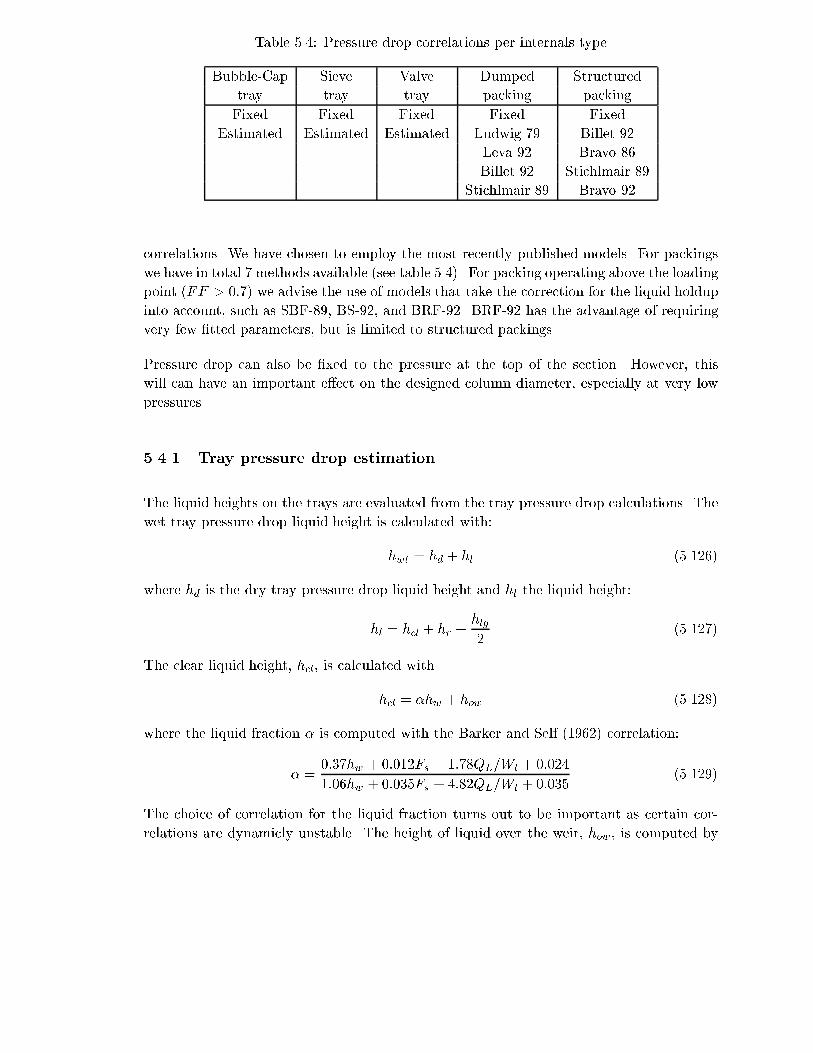
p
Table 5.4: Pressure drop correlations per internals type
Bubble-Cap Sieve Valve Dumped Structured
tray tray tray packing packing
Fixed Fixed Fixed Fixed Fixed
Estimated Estimated Estimated Ludwig 79 Billet 92
Leva 92 Bravo 86
Billet 92 Stichlmair 89
Stichlmair 89 Bravo 92
correlations. We have chosen to employ the most recently published models. For packings
we have in total 7 methods available (see table 5.4). For packing operating above the loading
point (FF > 0:7) we advise the use of models that take the correction for the liquid holdup
into account, such as SBF-89, BS-92, and BRF-92. BRF-92 has the advantage of requiring
very few �tted parameters, but is limited to structured packings.
Pressure drop can also be �xed to the pressure at the top of the section. However, this
will can have an important e�ect on the designed column diameter, especially at very low
pressures.
5.4.1 Tray pressure drop estimation
The liquid heights on the trays are evaluated from the tray pressure drop calculations. The
wet tray pressure drop liquid height is calculated with:
hwt = hd + hl (5.126)
where hd is the dry tray pressure drop liquid height and hl the liquid height:
hl = hcl + hr +hlg
2(5.127)
The clear liquid height, hcl, is calculated with
hcl = �hw + how (5.128)
where the liquid fraction � is computed with the Barker and Self (1962) correlation:
� =0:37hw + 0:012Fs + 1:78QL=Wl + 0:024
1:06hw + 0:035Fs + 4:82QL=Wl + 0:035(5.129)
The choice of correlation for the liquid fraction turns out to be important as certain cor-
relations are dynamicly unstable. The height of liquid over the weir, how, is computed by

p q
various correlations for di�erent types of weirs (see Perry) and a weir factor (Fw) correction
(see Smith, pp. 487) is employed. For example for a segmental weir:
how = 0:664Fw
�QL
Wl
�2=3(5.130)
w =Wl
Dc
(5.131)
F 3w =
w2
1� (Fww(1:68QL
W 2:5l
)2=3 +p1� w2)2
(5.132)
where QL is the volumetric ow over the weir per weir length. The residual height, hr, is
only taken into account for sieve trays. Bennett's method (see Lockett, pp. 81) is:
hr =
�6
1:27�L
���
g
�2=3 ��L � �V
dh
�1=3(5.133)
Dry tray pressure, hd, is calculated with:
hd = K�G
�Lu2h (5.134)
K =�
2g(5.135)
where the orri�ce coe�cient � for sieve trays is computed according to Stichlmair and
Mersmann (1978). For valve trays we use the method of Klein (1982) as described in Kister
(1992, pp. 309{312) where K is given for the cases with the valves closed or open. It is
extended for double weight valve trays as discussed by Lockett (1986, pp. 82{86). The dry
tray pressure drop is corrected for liquid fractional entrainment.
The froth density is computed with
hf =hcl
�(5.136)
The liquid gradient, hlg, is computed according to Fair (Lockett, 1986, pp. 72):
Rh =Whf
W + 2hf(5.137)
Uf =QL
Whcl(5.138)
Ref =RhUf�L
�L(5.139)
f = 7 104hwRe�1:06f
(5.140)
hlg =ZfU2
f
gRh
(5.141)
where W is the average ow-path width for liquid ow, and Z the ow path length. The
height of liquid at the tray inlet is:
hi =
s2
g
�QL
Wl
�2 � 1
hcl�
1
hc
�+2�h2
f
3(5.142)
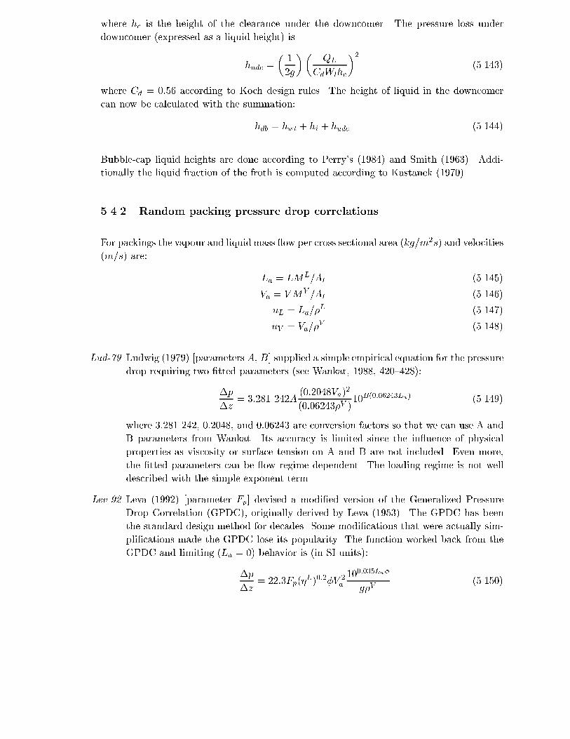
p
where hc is the height of the clearance under the downcomer. The pressure loss under
downcomer (expressed as a liquid height) is
hudc =
�1
2g
��QL
CdWlhc
�2(5.143)
where Cd = 0:56 according to Koch design rules. The height of liquid in the downcomer
can now be calculated with the summation:
hdb = hwt + hi + hudc (5.144)
Bubble-cap liquid heights are done according to Perry's (1984) and Smith (1963). Addi-
tionally the liquid fraction of the froth is computed according to Kastanek (1970).
5.4.2 Random packing pressure drop correlations
For packings the vapour and liquidmass ow per cross sectional area (kg=m2s) and velocities
(m=s) are:
La = LML=At (5.145)
Va = VMV =At (5.146)
uL = La=�L (5.147)
uV = Va=�V (5.148)
Lud-79 Ludwig (1979) [parameters A, B] supplied a simple empirical equation for the pressure
drop requiring two �tted parameters (see Wankat, 1988, 420{428):
�p
�z= 3:281 242A
(0:2048Va)2
(0:06243�V )10B(0:06243La) (5.149)
where 3:281 242, 0:2048, and 0:06243 are conversion factors so that we can use A and
B parameters from Wankat. Its accuracy is limited since the in uence of physical
properties as viscosity or surface tension on A and B are not included. Even more,
the �tted parameters can be ow regime dependent. The loading regime is not well
described with the simple exponent term.
Lev-92 Leva (1992) [parameter Fp] devised a modi�ed version of the Generalized Pressure
Drop Correlation (GPDC), originally derived by Leva (1953). The GPDC has been
the standard design method for decades. Some modi�cations that were actually sim-
pli�cations made the GPDC lose its popularity. The function worked back from the
GPDC and limiting (La = 0) behavior is (in SI units):
�p
�z= 22:3Fp(�
L)0:2�V 2a
100:035La�
g�V(5.150)

p q
with � = �water=�l = 1000=�l . This result is similar to the Ludwig (1979) equation
with corrections for the in uence of the liquid density and viscosity. The only parame-
ter is the packing factor Fp which can be obtained from dry pressure drop experiments
(see Leva, 1992) or computed by the speci�c packing area over the void fraction cubed.
Again, the loading regime is not well described with the simple exponent term. This is
model is the default pressure drop model for random packings if no model is speci�ed,
since it requires only the packing factor.
SBF-89 Stichlmair et al. (1989) [parameters ap, �, C1, C2, C3] published a semi-empirical
method from an analogy of the friction of a bed of particles and the pressure drop.
It contains a correction for the actual void fraction corrected for the holdup, which is
dependent on the pressure drop. Therefore, it is an iterative method. It is suitable
for both random and structured packings, but there are few published parameters for
structured packings. The pressure drop is
�p
�z= 0:75f0(1� �p)�
V � U2V =(dp�
4:65p ) (5.151)
where the void fraction of the irrigated bed, equivalent packing diameter, Reynolds
number, and friction factor for a single particle are:
�p = �� ht (5.152)
dp = 6(1� �p)ap (5.153)
ReV = uV dp�V =�V (5.154)
f0 = C1=ReV + C2=pReV + C3 (5.155)
Iteration is started by assuming a dry bed for which �p = � and the holdup fraction is
computed with the liquid Froude number:
FrL = u2Lap=g�4:65 (5.156)
ht = 0:555Fr1=3L
(5.157)
The liquid holdup is limited to 0:5 in order to handle ooding.
BS-92 Billet and Schultes (1992) and Billet's monograph (1979?) [parameters a, �, Cfl,
Ch, Cp] include a extensive model and an extensive lists of packing data with �tted
parameters. The method is rather complicated but has two regimes. The method
does correct for the holdup change in the loading regime but employs an empirical
exponential term, and is not iterative.
Packing dimension, hydraulic diameter and F-factor are
dp = 6(1 � �)=ap (5.158)
dh = 4�=ap (5.159)
Fs = uV
q�V (5.160)
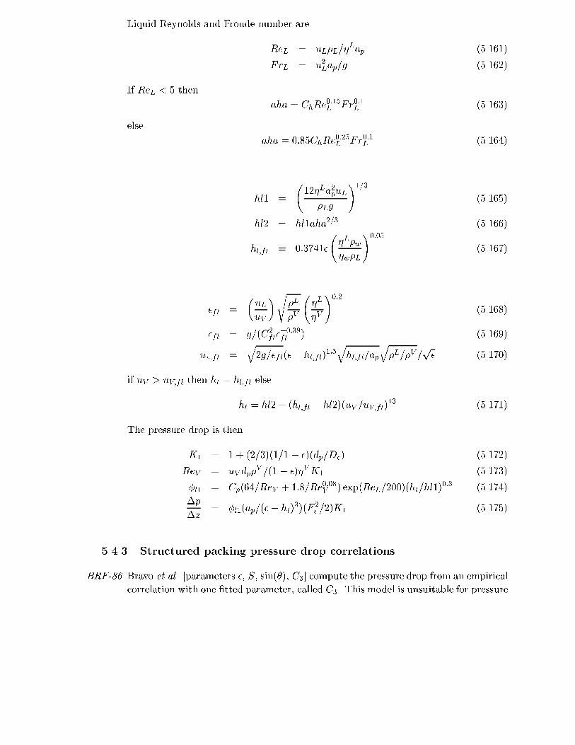
p
Liquid Reynolds and Froude number are
ReL = uL�L=�Lap (5.161)
FrL = u2Lap=g (5.162)
If ReL < 5 then
aha = ChRe0:15L Fr0:1L (5.163)
else
aha = 0:85ChRe0:25L Fr0:1L (5.164)
hl1 =
12�La2puL
�Lg
!1=3
(5.165)
hl2 = hl1aha2=3 (5.166)
hl;fl = 0:3741�
�L�w
�w�L
!0:05
(5.167)
�fl =
�uL
uV
�s�L
�V
�L
�V
!0:2
(5.168)
�fl = g=(C2fl�
�0:39fl
) (5.169)
uv;fl =q2g=�fl(�� hl;fl)
1:5qhl;fl=ap
q�L=�V =
p� (5.170)
if uV > uV;fl then ht = hl;fl else
ht = hl2 + (hl;fl � hl2)(uV =uV;fl)13 (5.171)
The pressure drop is then
K1 = 1 + (2=3)(1=1 � �)(dp=Dc) (5.172)
ReV = uV dp�V =(1� �)�VK1 (5.173)
�l1 = Cp(64=ReV + 1:8=Re0:08V ) exp(ReL=200)(ht=hl1)0:3 (5.174)
�p
�z= �l1(ap=(�� ht)
3)(F 2s =2)K1 (5.175)
5.4.3 Structured packing pressure drop correlations
BRF-86 Bravo et al. [parameters �, S, sin(�), C3] compute the pressure drop from an empirical
correlation with one �tted parameter, called C3. This model is unsuitable for pressure

p q
drop correlations in the loading regime (FF > 0:7). The pressure drop per height of
packing is:
�p
�z= (0:171 + 92:7=ReV )(�
V u2V;eff=deq)(1
(1 � C3
pFr)
)5 (5.176)
where
uV;eff = uV =(� sin �) (5.177)
ReV =deq�
V uV;eff
�V(5.178)
FrL = u2L=deqg (5.179)
SBF-92 Stichlmair et al. (1989) [parameters a, �, C1, C2, C3] published a semi-empirical
method, see the section on pressure drop of random packed columns above.
BRF-92 Bravo et al. (1992) [parameters ap, �, S, �, K2, dPdzflood] developed a theoretical
model developed for modern structured packings. Two parameters need to be supplied
for pressure drop calculations, however, the K2 parameter was �tted by the authors.
The pressure of ooding (dPdzflood) can be easily obtained from data or via Kister's
correlation and the packing factor. The model includes an iterative method with a
dependence of the liquid holdup on the pressure drop (and vice versa). The Weber,
Froude, and Reynolds numbers are
WeL = u2L�LS=� (5.180)
FrL = u2L=(Sg) (5.181)
ReL = uLS�L=�L (5.182)
The e�ective g (as a function of ht) is calculated:
geff =
1�
dPdZ
dPdZflood
!(�L � �V )
�Lg (5.183)
Then Ft (see above), ht, and dPdZ are computed
ht =
�4Ft
S
�2=3 3�LuL
�V sin ��geff
!1=3
(5.184)
A =0:177�V
S�2(sin �)2(5.185)
B =88:774�V
S2� sin �(5.186)
�p
�z= (Au2V +BuV )
�1
1�K2ht
�5(5.187)
The calculation is repeated until pressure drop converges or when it becomes larger
than the pressure drop at ood. The iteration can actually have problems in conver-
gencing.

p g
BS-92 Billet and Schultes (1992) and Billet's monograph (1979?) [ap, �, Cf l, Ch, Cp] include
a extensive model, see the section on pressure drop of random packed columns above.
5.5 Entrainment and Weeping
Entrainment and weeping ows (for trays only) change the internal liquid ows and in uence
the performance of the column internals. ChemSep currently does not support the
handling of these ows. This is due to the fact that few entrainment models behave
properly. Neither is the e�ect of the entrainment and weep ows on the mass transfer
properly taken into account.
Entrainment is computed from the fractional liquid entrainment which is computed from
Hunt's correlation and from �gure 5.11 of Lockett (1986) for sieve trays:
�L = 7:75 10�5�0:073
�
�Mv
�Uv
Ts � 2:5hcl
�3:2(5.188)
The weeping factor is estimated from a �gure from Smith (1963, plot on page 548), which
was �tted with the following correlation
WF =0:135 � ln(34(Hw +How) + 1)
(Hd +Hr)(5.189)
where � is the open area ratio.
5.6 The Design Mode
The initial layout is determined after the ows are known from the initial guess. Each
stage in the column is designed separately and independently of adjacent stages. Then
the sections in the column are rationalized so that trays or stages within a section have the
same layout. During each iteration (that is, an update of the ows) each stage is re-designed
only if the owrates have changed more than by a certain fraction (which can be speci�ed).
Only sections with re-designed trays or stages are rationalized again. After convergence a
complete design of any trayed or packed section in the column is obtained. In this manner
trayed and packed sections can be freely mixed in a column simulation/design.
Di�erent design methods can be employed:
� Fraction of ooding; this is the standard design method for trays, we have employed
a modi�ed version of the method published by Barnicki and Davis (1989).

p q
� Pressure drop; this is the usual design method for packed columns, but is very useful
as well for tray design with pressure drop constraints.
� Optimizing; a `new' way of designing columns that incorporates the di�erent design
considerations in a more rigorous manner than conventional design algorithms. It is
more computationally intensive than the other two methods and only applicable for
tray sections.
The methods generate a column-design that might not be optimal from an engineers view-
point. They must be seen as starting points for the actual design layouts. Also, the design
does not include constructional calculations to determine tray support constructions or
thicknesses of trays or the column. Design mode is automatically triggered if the column
diameter is not speci�ed. Other layout parameters can be speci�ed but they may be changed
by the design mode. Each of these methods behaves di�erently and they are discussed in
more detail below. An additional and very important de-rating factor is the system factor
(SF). It represents the uncertaincy in design correlations with regard to phenomena which
are currently still not properly modeled, such as foaming.
Tray layout parameters that specify a complete design (for the calculation of mass transfer
coe�cients and pressure drops) are shown in Table 5.5. For packings only the column
diameter and bed height are design parameters, other parameters are �xed with the selection
of the type of packing (such as void fraction, nominal packing diameter, etc.). The packed
bed height must be speci�ed since it determines the desired separation and the capacity.
5.6.1 Tray Design: Fraction of ooding
The �rst task in this approach to tray design is to assign all layout parameters to consistent
values corresponding to the required capacity de�ned by the fraction of ooding and current
owrates. These defaults function as starting points for subsequent designs.
The initial free area ratio is taken to be 15 % of the active area. The active area is determined
with capacity factor calculation with internals speci�c methods (for sieve and bubble-cap
trays the default is Fair's correlation by Ogboja and Kuye (19), and the Glitsch method
for valve trays). The tray spacing is initially set to the default value (of 0:5m) and the
downcomer area is calculated according the Glitsch manual (limited by a minimum time
residence check). From the combined areas the column diameter is computed. The number
of liquid passes on a tray is initially set by the column diameter; under 5ft one pass, under
8ft two, 10ft three, under 13ft four, else �ve passes. With the number of passes and the
column diameter the total weir length is computed. Once the weir length is determined the
liquid weir load is checked, if too high the number of passes is incremented and a new weir
length is evaluated until the weir load is below a speci�ed maximum.

g
Table 5.5: Tray layout data
General (sieve) tray layout data:
Column diameter Active area
Number of ow passes Total hole area
Tray spacing Downcomer area
Liquid ow path length Weir length
Hole diameter Weir height
Hole pitch Deck thickness
Downcomer clearance
Additional data for bubble caps:
Cap diameter Slot area
Slot height Riser area
Skirt clearance Annual area
Additional data for valves:
Closed Loss K Open Loss K
Eddy Loss C Ratio Valve Legs
Valve Density Valve Thickness
Fraction Heavy Valves Heavy Valve Thickness
Initial weir height is taken as 2", but limited to a maximum of 15 % of the tray spacing.
For notched or serrated weirs the notch depth is a third of the weir height. For serrated
weirs the angle of serration is 45 degrees. Circular weirs have diameters 0.9 times the weir
length. Hole diameter is set to 3/16" for sieve trays and tray thickness 0.43 times the hole
diameter (or 1/10"). The hole pitch is computed from the free area ratio and hole diameter
according to a triangular pitch. The default downcomer clearance is 1.5" but is limited by
the maximum allowed downcomer velocity according to the Glitch method de-rated with
the system factor. The clearance is set to be at least half an inch lower than the weir height
to maintain a positive liquid seal but is limited to a minimum of half an inch.
For bubble-cap trays the cap diameter is 3" for column diameters below 4.5 ft and 4" for
above. The hole diameter can vary between 60 % to 71 % of the capdiameter, and default
taken as 70 %. Default skirt clearance is 1" with minimum of 0.5" and maximum of 1.5".
slot height can vary in between 0.5" and 1.5", default 1" for cap diameters below 3.5" and
1.25" for larger cap diameters. The pitch can vary from 1.25" to half the ow path length
(minimum number of rows is two), default set to 1.25".
Valve trays are initialized to be Venturi ori�ce uncaged, carbon steel valves of 3 mm thick
with 3 legs (see Kister, 1992, p312). The hole diameter is 1" for column smaller than 4.5
ft, otherwise 2". No double weight valves are present.

p q
The second task in the fraction of ooding method consists of �nding the proper free area
ratio (� = Ah=Ab = hole area / active area) so that no weeping occurs. This ratio can
vary between a minimum of 5% (for stable operation) and a maximum of 20%. To test
whether weeping occurs, we use the correlation by Lockett and Banik (1984): Frhole > 2=3.
The method requires all liquid heights to be evaluated at weep rate conditions. This task
is ignored for bubble-cap trays. The weep test is done at weeping conditions, with a weep
factor at 60 % (this can be changed). Calculating liquid heights is done by adding various
contributions with correlations from Lockett (1986) and Kister (1992), see Appendix A. If
weeping occurs at the lower bound for the free area ratio, a ag is set for the �nal task to
adapt the design.
The �nal task consists of evaluating all liquid heights at normal conditions and to do a
number of checks:
� vapor distribution (for bubble-caps),
� weeping (for sieve/valve trays),
� hydraulic ooding,
� excessive liquid entrainment,
� froth height limit, and
� excessive pressure drop
If a check fails the design is adapted to correct the problem, according to the adjustments
shown in Table 5.6 after which new areas are calculated with capacity correlations. Part of
this task is also to keep the layout parameters that are adjusted within certain lower and
upper bounds to maintain a proper tray design. Finally the number of iterations for the
design method is checked against a maximum (default 30) to prevent a continuous loop.
The adjustment factors f1, f2, and f3 are percentual in/decrements, normally set at 5, 2,
and 1 %. These factors { together with all the default, lower, and upper settings that
are used in the design routine { are stored in a \design �le" (TDESIGN.DEF) that can
be tailored to handle speci�c kinds of designs and columns. This allows the selection of
di�erent methods for capacity and hydrodynamic calculations as well. Also the fraction
that the ows need to change before a re-design is issued can be changed in this manner
together with other design criteria. The design �le must be in the current directory for the
nonequilibrium program to use it, otherwise the normal defaults will be used.
Here we discuss the most important parameters of the �le. The �le starts with a comment
on the �rst line. The second line speci�es the factors f1, f2, and f3 for adapting the design
layout parameters. The third line speci�es the fraction of change allowed in the ows
before a redesign occurs. It also speci�es the fraction of deviation allowed in downcomer

g
Table 5.6: Tray design checks and adjustments
Problem Test Adjustments
Bubble cap vapor distribution hlg=hd > 0:5 p+ f1,
hskirt + f2,
hslot + f3,
dh � f3
Weeping Frh=(2=3) < 1� fafree < 0:05
Ab < Abf : Ab = Abf
Wf + f1else: Ab � f1
dh � f3hw � f3
tv + f2 (vt)
Hydrodynamic (downcomer) ooding) Ts < hdb=FF Ts + f1Ad + f1hw + f2hc + f3
Excessive liquid entrainment Ab + f1Ts + f1dh � f2hw � f3
Froth height limit hf > 0:75Ts Ab + f1Ts + f2hw � f3
Excessive pressure drop g�hwt > �pmax Ab + f1hw � f1dh + f2
p+ f1 (bc)
hskirt + f2 (bc)
hslot + f3 (bc)
Excessive vapor entrainment Ad + f1
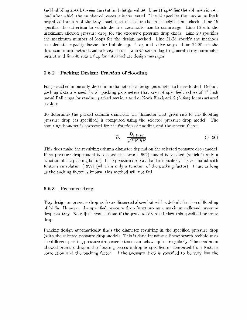
p q
and bubbling area between current and design values. Line 11 speci�es the volumetric weir
load after which the number of passes is incremented. Line 14 speci�es the maximum froth
height as fraction of the tray spacing as is used in the froth height limit check. Line 15
speci�es the criterium to which the free area ratio has to conmverge. Line 16 sets the
maximum allowed pressure drop for the excessive pressure drop check. Line 20 speci�es
the maximum number of loops for the design method. Line 21-23 specify the methods
to calculate capacity factors for bubble-cap, sieve, and valve trays. Line 24-25 set the
downcomer are method and velocity check. Line 45 sets a ag to generate tray parameter
output and line 46 sets a ag for intermediate design messages
5.6.2 Packing Design: Fraction of ooding
For packed columns only the column diameter is a design parameter to be evaluated. Default
packing data are used for all packing parameters that are not speci�ed; values of 1" inch
metal Pall rings for random packed sections and of Koch Flexipack 2 (316ss) for structured
sections.
To determine the packed column diameter, the diameter that gives rise to the ooding
pressure drop (as speci�ed) is computed using the selected pressure drop model. The
resulting diameter is corrected for the fraction of ooding and the system factor:
Dc =Dc;floodpFF SF
(5.190)
This does make the resulting column diameter depend on the selected pressure drop model.
If no pressure drop model is selected the Leva (1992) model is selected (which is only a
function of the packing factor). If no pressure drop at ood is speci�ed, it is estimated with
Kister's correlation (1992) (which is only a function of the packing factor). Thus, as long
as the packing factor is known, this method will not fail.
5.6.3 Pressure drop
Tray design on pressure drop works as discussed above but with a default fraction of ooding
of 75 %. However, the speci�ed pressure drop functions as a maximum allowed pressure
drop per tray. No adjustment is done if the pressure drop is below this speci�ed pressure
drop.
Packing design automatically �nds the diameter resulting in the speci�ed pressure drop
(with the selected pressure drop model). This is done by using a linear search technique as
the di�erent packing pressure drop correlations can behave quite irregularly. The maximum
allowed pressure drop is the ooding pressure drop as speci�ed or computed from Kister's
correlation and the packing factor. If the pressure drop is speci�ed to be very low the
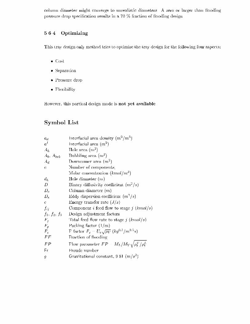
g
column diameter might converge to unrealistic diameters. A zero or larger than ooding
pressure drop speci�cation results in a 70 % fraction of ooding design.
5.6.4 Optimizing
This tray design only method tries to optimize the tray design for the following four aspects:
� Cost
� Separation
� Pressure drop
� Flexibility
However, this partical design mode is not yet available.
Symbol List
ad Interfacial area density (m2=m3)
aI Interfacial area (m2)
Ah Hole area (m2)
Ab, Abub Bubbling area (m2)
Ad Downcomer area (m2)
c Number of components,
Molar concentration (kmol=m3)
dh Hole diameter (m)
D Binary di�usivity coe�cient (m2=s)
Dc Column diameter (m)
De Eddy dispersion coe�cient (m2=s)
e Energy transfer rate (J=s)
fij Component i feed ow to stage j (kmol=s)
f1, f2, f3 Design adjustment factors
Fj Total feed ow rate to stage j (kmol=s)
Fp Packing factor (1=m)
Fs F factor Fs = Uvp�V (kg0:5=m0:5s)
FF Fraction of ooding
FP Flow parameter FP =ML=MV
q�Vt =�
Lt
Fr Froude number
g Gravitational constant, 9.81 (m=s2)
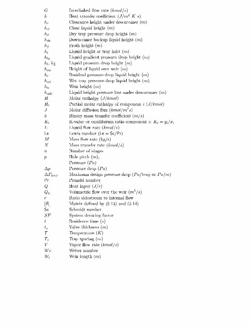
p q
G Interlinked ow rate (kmol=s)
h Heat transfer coe�cient (J=m2 K s)
hc Clearance height under downcomer (m)
hcl Clear liquid height (m)
hd Dry tray pressure drop height (m)
hdb Downcomer backup liquid height (m)
hf Froth height (m)
hi Liquid height at tray inlet (m)
hlg Liquid gradient pressure drop height (m)
hl, hL Liquid pressure drop height (m)
how Height of liquid over weir (m)
hr Residual pressure drop liquid height (m)
hwt Wet tray pressure drop liquid height (m)
hw Weir height (m)
hudc Liquid height pressure loss under downcomer (m)
H Molar enthalpy (J=kmol)�Hi Partial molar enthalpy of component i (J=kmol)
J Molar di�usion ux (kmol=m2s)
k Binary mass transfer coe�cient (m=s)
Ki K-value or equilibrium ratio component i: Ki = yi=xiL Liquid ow rate (kmol=s)
Le Lewis number (Le = Sc=Pr)
M Mass ow rate (kg/s)
N Mass transfer rate (kmol=s)
n Number of stages
p Hole pitch (m),
Pressure (Pa)
�p Pressure drop (Pa)
�Pmax Maximum design pressure drop (Pa=tray or Pa=m)
Pr Prandtl number
Q Heat input (J=s)
QL Volumetric ow over the weir (m3=s)
r Ratio sidestream to internal ow
[R] Matrix de�ned by (5.13) and (5.14)
Sc Schmidt number
SF System derating factor
t Residence time (s)
tv Valve thickness (m)
T Temperature (K)
Ts Tray spacing (m)
V Vapor ow rate (kmol=s)
We Weber number
Wl Weir length (m)
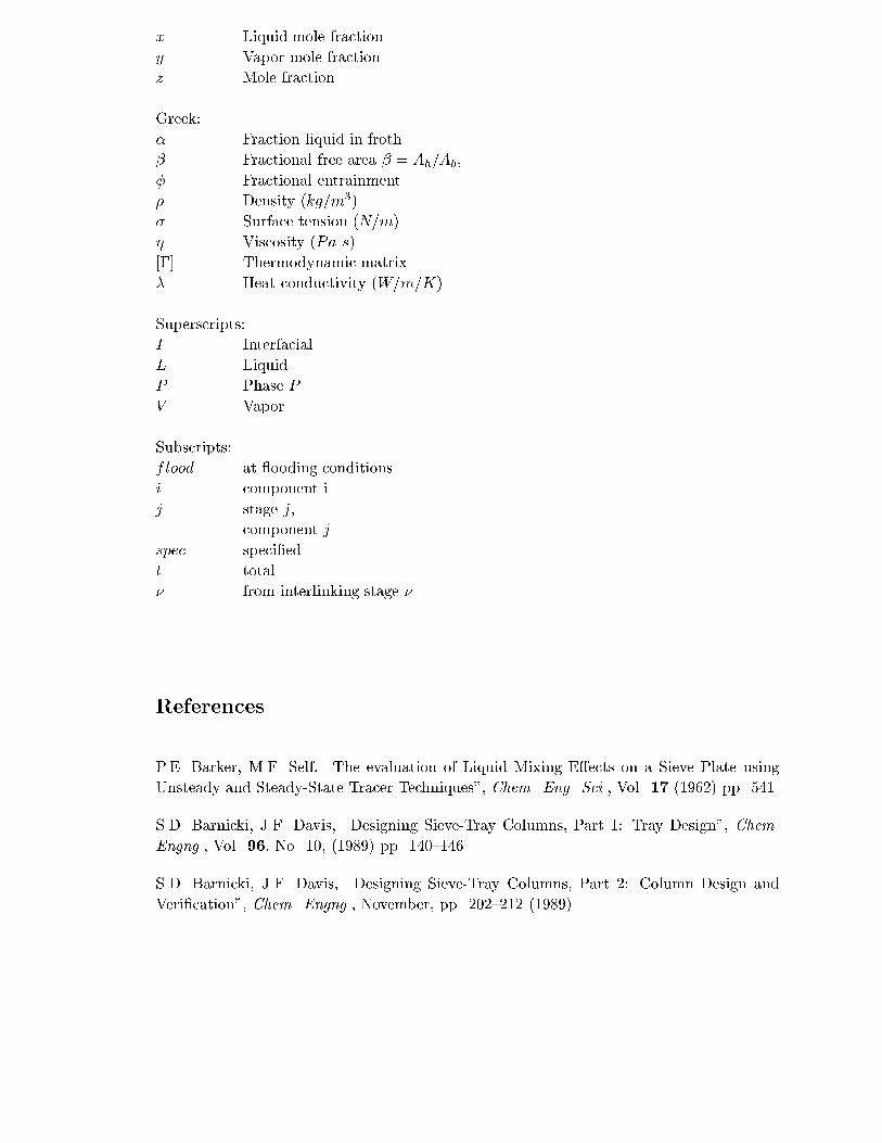
x Liquid mole fraction
y Vapor mole fraction
z Mole fraction
Greek:
� Fraction liquid in froth
� Fractional free area � = Ah=Ab,
� Fractional entrainment
� Density (kg=m3)
� Surface tension (N=m)
� Viscosity (Pa s)
[�] Thermodynamic matrix
� Heat conductivity (W=m=K)
Superscripts:
I Interfacial
L Liquid
P Phase P
V Vapor
Subscripts:
flood at ooding conditions
i component i
j stage j,
component j
spec speci�ed
t total
� from interlinking stage �
References
P.E. Barker, M.F. Self, \The evaluation of Liquid Mixing E�ects on a Sieve Plate using
Unsteady and Steady-State Tracer Techniques", Chem. Eng. Sci., Vol. 17 (1962) pp. 541.
S.D. Barnicki, J.F. Davis, \Designing Sieve-Tray Columns, Part 1: Tray Design", Chem.
Engng., Vol. 96, No. 10, (1989) pp. 140{146.
S.D. Barnicki, J.F. Davis, \Designing Sieve-Tray Columns, Part 2: Column Design and
Veri�cation", Chem. Engng., November, pp. 202{212 (1989).
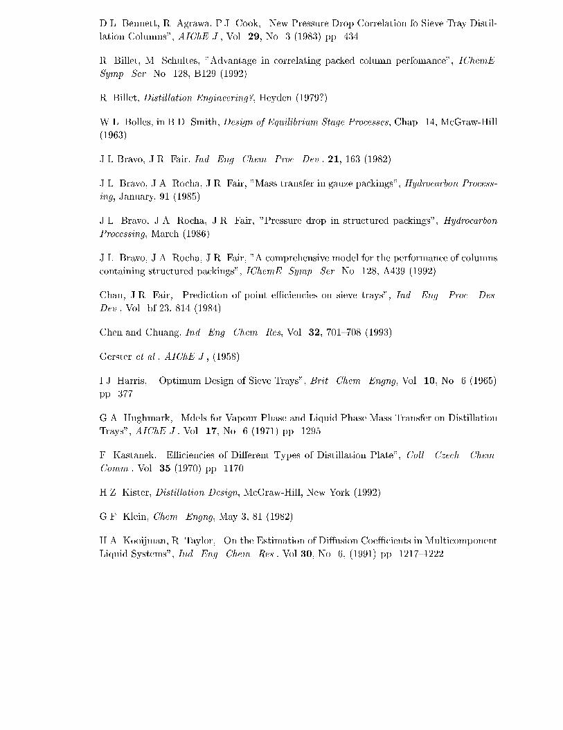
p q
D.L. Bennett, R. Agrawa, P.J. Cook, \New Pressure Drop Correlation fo Sieve Tray Distil-
lation Columns", AIChE J., Vol. 29, No. 3 (1983) pp. 434.
R. Billet, M. Schultes, "Advantage in correlating packed column perfomance", IChemE.
Symp. Ser. No. 128, B129 (1992).
R. Billet, Distillation Engineering?, Heyden (1979?).
W.L. Bolles, in B.D. Smith, Design of Equilibrium Stage Processes, Chap. 14, McGraw-Hill
(1963).
J.L Bravo, J.R. Fair, Ind. Eng. Chem. Proc. Dev., 21, 163 (1982).
J.L. Bravo, J.A. Rocha, J.R. Fair, "Mass transfer in gauze packings", Hydrocarbon Process-
ing, January, 91 (1985).
J.L. Bravo, J.A. Rocha, J.R. Fair, "Pressure drop in structured packings", Hydrocarbon
Processing, March (1986).
J.L. Bravo, J.A. Rocha, J.R. Fair, "A comprehensive model for the performance of columns
containing structured packings", IChemE. Symp. Ser. No. 128, A439 (1992).
Chan, J.R. Fair, \Prediction of point e�ciencies on sieve trays", Ind. Eng. Proc. Des.
Dev., Vol. bf 23, 814 (1984)
Chen and Chuang, Ind. Eng. Chem. Res, Vol. 32, 701{708 (1993).
Gerster et al., AIChE J., (1958).
I.J. Harris, \ Optimum Design of Sieve Trays", Brit. Chem. Engng, Vol. 10, No. 6 (1965)
pp. 377.
G.A. Hughmark, \Mdels for Vapour Phase and Liquid Phase Mass Transfer on Distillation
Trays", AIChE J., Vol. 17, No. 6 (1971) pp. 1295.
F. Kastanek, \E�ciencies of Di�erent Types of Distillation Plate", Coll. Czech. Chem.
Comm., Vol. 35 (1970) pp. 1170.
H.Z. Kister, Distillation Design, McGraw-Hill, New York (1992).
G.F. Klein, Chem. Engng, May 3, 81 (1982).
H.A. Kooijman, R. Taylor, \On the Estimation of Di�usion Coe�cients in Multicomponent
Liquid Systems", Ind. Eng. Chem. Res., Vol 30, No. 6, (1991) pp. 1217{1222.

W.J. Korchinsky, \Liquid Mixing in Distillation Trays: Simultaneous Measurement of the
Di�usion Coe�cient and Point E�ciency", Trans. I. Chem. E., Vol. 72, Part A, (1994)
472-478.
R. Krishnamurthy, R. Taylor, \A Nonequilibrium Stage Model of Multicomponent Separa-
tion Processes. Part I: Model Description and Method of Solution", AIChE J., Vol. 31,
No. 3 (1985), pp. 449{455.
Leva, (1953?).
M. Leva, \Reconsider Packed-Tower Pressure-Drop correlations", Chem. Eng. Prog. Jan-
uary, 65 (1992).
M.J. Lockett, Distillation Tray Fundamentals, Cambridge University Press (1986).
M.J. Lockett, S. Banik, \Weeping from Sieve Trays", AIChE Meeting, San Francisco, Nov.
(1984).
E.E. Ludwig, Applied Process Design for Chemical and Petrochemical Plants, Vol. 2, 2nd
Ed., Gulf Pub. Co., Houston, TX, (1979).
O. Ogboja, A. Kuye, \A procedure for the design and optimisation of sieve trays", Trans.
I. Chem. E., Vol. 68, Part A, Sept. (1990) pp. 445-452.
K. Onda, H. Takeuchi, Y. Okumoto, "Mass transfer coe�cients between gas and liquid
phases in packed columns", J. Chem. Eng. Jap., Vol. 1, No.1, 56 (1968).
R.H. Perry and D. Green,Perry's Chemical Engineering Handbook, 6th edition, section 18,
Liquid-Gas System, 18-8 { 18-12 (1984).
M. Prado, The bubble-to-Spray Transition on Sieve Trays: Mechanisms of the Phase Inver-
sion, Ph.D. thesis, University of Texas, Austin (1986).
B.D. Smith, Design of Equilibrium Staged Processes, McGraw-Hill, New York (1963)
J. Stichlmair, A. Mersmann, \Dimensioning Plate Columns for Absorption and Recti�ca-
tion", Chem. Ing. Tech., Vol. 45, No. 5 (1978) pp. 242.
J. Stichlmair, J.L. Bravo, J.R. Fair, Gas. Sep. Purif., Vol. 3, 19 (1989).
R. Taylor, H.A. Kooijman, \Composition derivatives of Activity Models (for the estimation
of Thermodynamic Factors in Di�usion)", Chem. Eng. Comm., Vol. 102 (1991) pp. 87{
106.
R. Taylor, H.A. Kooijman, J-S. Hung, \A second generation nonequilibrium model for

p q
computer simulation of multicomponent separation processes", Comput. Chem. Engng.,
Vol. 18, No. 3, pp. 205{217 (1994).
R. Taylor, R. Krishna, Multicomponent Mass Transfer, Wiley, New York (1993).
P.C. Wankat, Separations in Chemical Engineering - Equilibrium Staged Separations, Else-
vier, 420{428 (1988).
F.J. Zuiderweg, \Sieve Trays - A View of the State of the Art", Chem. Eng. Sci., 37,
1441{1461 (1982).

Chapter 6
Nonequilibrium Extraction
This chapter deals especially with the application of the nonequilibrium model to the mod-
elling of extraction columns. In such operations the two phases present are both liquids
instead of a liquid and a vapor as in the case of distillation, stripping, or absorption. This
requires fundamentally di�erent mass transfer coe�cients and ow models, as well as a
completely new design method, that an entire chapter is devoted to the subject.
6.1 Introduction
Nonequilibrium extraction uses the same model as described in the nonequilibrium section,
with the exception that there is no vapor. Instead we have a light and a heavy liquid
phase, where the light liquid behaves as the vapor with, of course, liquid-like properties.
If the heavy phase (L) is lighter than the light phase (V) the program stops. However,
either phase (that is, L or V) can be the disperse phase. The user must specify which is
the disperse phase, since this changes the design and the calculation of MTC's. Currently
sieve trays, structured and random packed columns, rotating disc contacters, and spray
columns are supported as internals (as well as equilibrium stages with a speci�ed stage
e�ciency). The K-values must be the Liquid-Liquid model, which uses activity coe�cients.
The energy balance can be ignored (Enthalpy=None) or included. In case it is ignored the
column temperature is dictated by that of the feeds, and linear interpolation is used to
provide a column temperature pro�le. A speci�c temperature pro�le can be imposed if the
energy balance is ignored and user temperature initialization is supplied. Default values
for the total interfacial area and mass transfer coe�cients are: Ai = 100 m2, kd = 10�5
and kc = 10�4 m=s. Mass transfer in coelescencing layers and jet zones are neglected (they
could be modeled by a special stage for packed/RDC columns). Thus, only the drop rise
zone is taken into account for mass transfer.
91
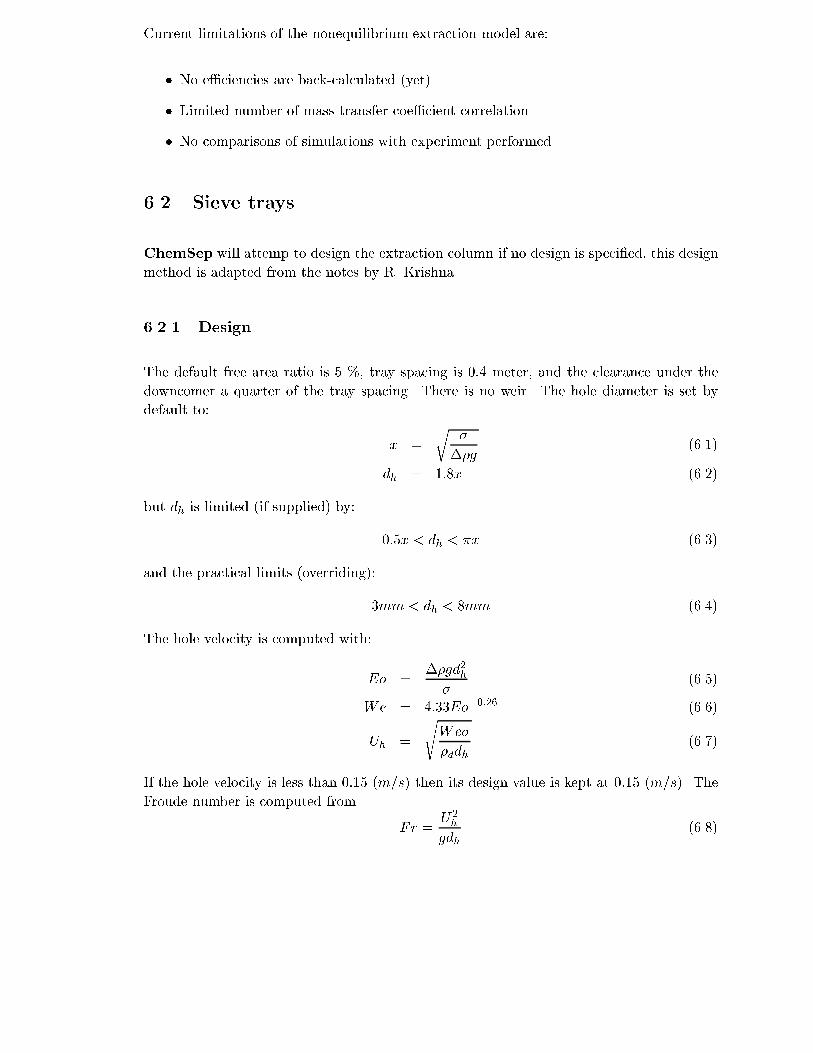
p q
Current limitations of the nonequilibrium extraction model are:
� No e�ciencies are back-calculated (yet)
� Limited number of mass transfer coe�cient correlation
� No comparisons of simulations with experiment performed
6.2 Sieve trays
ChemSep will attemp to design the extraction column if no design is speci�ed, this design
method is adapted from the notes by R. Krishna.
6.2.1 Design
The default free area ratio is 5 %, tray spacing is 0:4 meter, and the clearance under the
downcomer a quarter of the tray spacing. There is no weir. The hole diameter is set by
default to:
x =
r�
��g(6.1)
dh = 1:8x (6.2)
but dh is limited (if supplied) by:
0:5x < dh < �x (6.3)
and the practical limits (overriding):
3mm < dh < 8mm (6.4)
The hole velocity is computed with:
Eo =��gd2
h
�(6.5)
We = 4:33Eo�0:26 (6.6)
Uh =
sWe�
�ddh(6.7)
If the hole velocity is less than 0:15 (m=s) then its design value is kept at 0:15 (m=s). The
Froude number is computed from
Fr =U2h
gdh(6.8)
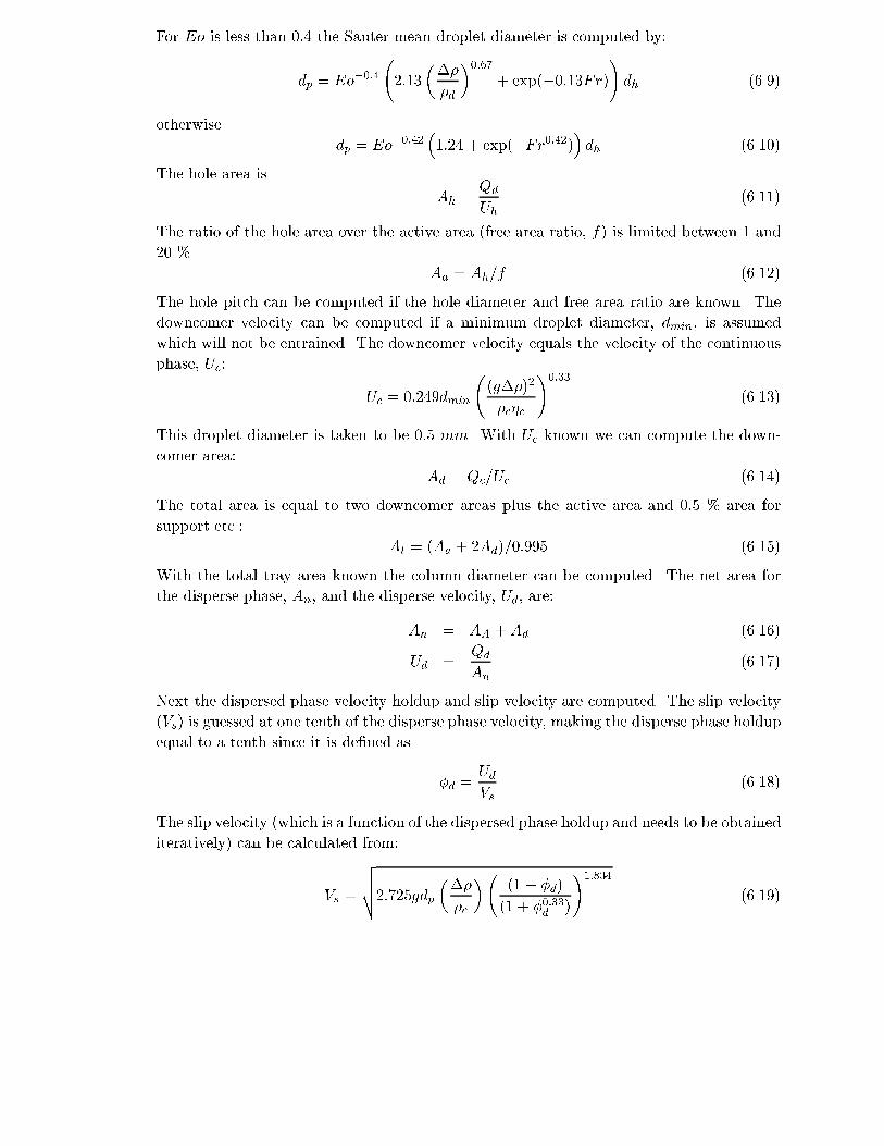
y
For Eo is less than 0:4 the Sauter mean droplet diameter is computed by:
dp = Eo�0:4 2:13
���
�d
�0:67+ exp(�0:13Fr)
!dh (6.9)
otherwise
dp = Eo�0:42�1:24 + exp(�Fr0:42)
�dh (6.10)
The hole area is
Ah =Qd
Uh(6.11)
The ratio of the hole area over the active area (free area ratio, f) is limited between 1 and
20 %.
Aa = Ah=f (6.12)
The hole pitch can be computed if the hole diameter and free area ratio are known. The
downcomer velocity can be computed if a minimum droplet diameter, dmin, is assumed
which will not be entrained. The downcomer velocity equals the velocity of the continuous
phase, Uc:
Uc = 0:249dmin
(g��)2
�c�c
!0:33
(6.13)
This droplet diameter is taken to be 0:5 mm. With Uc known we can compute the down-
comer area:
Ad = Qc=Uc (6.14)
The total area is equal to two downcomer areas plus the active area and 0:5 % area for
support etc.:
At = (Aa + 2Ad)=0:995 (6.15)
With the total tray area known the column diameter can be computed. The net area for
the disperse phase, An, and the disperse velocity, Ud, are:
An = AA +Ad (6.16)
Ud =Qd
An
(6.17)
Next the dispersed phase velocity holdup and slip velocity are computed. The slip velocity
(Vs) is guessed at one tenth of the disperse phase velocity, making the disperse phase holdup
equal to a tenth since it is de�ned as
�d =Ud
Vs(6.18)
The slip velocity (which is a function of the dispersed phase holdup and needs to be obtained
iteratively) can be calculated from:
Vs =
vuut2:725gdp
���
�c
� (1� �d)
(1 + �0:33d
)
!1:834
(6.19)

p q
After the dispersed phase holdup is computed (it depends on Vs) it is checked to be within 1
and 20 % for standard operation conditions. If it is too small the free area ratio is increased,
if it is too large the free area ratio is decreased (each by 5 %) till it is within the desired
range.
The Weber number
We = �dU2hdp=� (6.20)
must be larger than 2 to ensure all holes produce drops (i.e. to avoid inactive holes, see
Seibert and Fair, 1988).
The height of the coalesced layer is (according to Treybal, 1980):
hc =(U2
h� U2
d)�d
2gC2d��
+4:5Uc�c
2g��+
6�
dpg��(6.21)
(with Cd = 0:67). The �rst term is height to overcome ow through the orri�ces, the
second for friction losses due to contraction/expension on entry/exit (0:5 + 1:0) and change
of direction (2 times 1:5 velocity heads), and the third term for the interfacial tension e�ects
at the holes. The height needs to be larger than 4 cm (to ensure safe operation). If not,
then the hole diameter is decreased by 5 % and we repeat the procedure from the hole
velocity calculation (6.5).
This design is for a one pass sieve tray, and ow path length, Lf is computed from geometric
relations. The weir length is (segmental downcomer):
Wl = Aa=Lf (6.22)
The tray thickness is defaulted to a tenth of an inch. To prevent entrainment of droplets, the
ow under the downcomer is only allowed to be 50 % higher than the downcomer velocity.
If higher, then the downcomer clearance is enlarged until this requirement is met. The tray
spacing is adjusted so that the coeleseced layer and coalescence zone divided over the length
of the downcomer equals the fraction of ooding (multiplied with the system factor).
6.2.2 Report
The reported fraction of ooding equals to the ratio of the height of the coelesced layer
over the height of the downcomer (according to Seibert and Fair the ooding calculation
is within 20 %). The lower operating limit is the ratio of two over the Weber number (to
guarantee proper droplet formation).

6.2.3 Mass Transfer Coe�cients
The "Handlos-Baron-Treybal" method is used. The hole velocity Uh, Eo, Fr, net area An,
Sauter mean drop diameter dp, disperse velocity Ud, slip velocity Vs, disperse phase holdup
�d, hc, and hz are computed as above (but with �xed design parameters). The interfacial
area per unit of volume is
Ai =6�d
dp(6.23)
and the drop rising zone (where mass transfer is assumed to take place):
hdrop = ts � hc (6.24)
where ts is th etray spacing. The volume for mass transfer on a tray is
Vi = Anhdrop (6.25)
The mass transfer coe�cients for transport from the disperse phase are (Handlos and Baron,
1957):
kd =0:00375Vs
(1 + �d=�c)(6.26)
and for transport from the continuous phase are (Treybal, 1963):
kc;ij = 0:725Re�0:43c (1� �d)VsNu�0:58c (6.27)
with
Rec = dpVs�c=�c (6.28)
Nuc = �c=�cDc
ij (6.29)
Note that kd is not a function of the di�usion coe�cient and, thus, is the same for all
components.
6.3 Packed columns
Column design and calculation of mass transfer coe�cients is done the same way for struc-
tured packed column and random packed columns, following the methods and correlations
as outlined by Seibert and Fair (1988).
6.3.1 Design
For mass transfer from the continuous phase to the disperse phase we have x = 1 for the
calculation of the Sauter mean drop diameter:
dp = 1:15x
r�
��g(6.30)

p q
The slip velocity of a single droplet at zero disperse phase holdup is given by
V o
s =
s4��gdp
3�cCd(6.31)
where Cd = 0:38 (for high values of Reynolds). Static disperse holdup is:
�ds =0:076apdp
�(6.32)
where ap is the packing area and � the packing void fraction. The static holdup area and
total area are:
as = 60:076ap (6.33)
a = ap + as (6.34)
The tortuosity is de�ned as
� =adp
2(6.35)
The super�cial velocity of the continuous phase at the ood point is
e = cos(��
4) (6.36)
Ucf =0:192� � V o
s
(1:08 + (Qd=Qc)=e2)(6.37)
This needs to be corrected for the fraction of ooding (and system factor):
Uc = SF FF Ucf (6.38)
to give the net area
An =Qc
Uc(6.39)
from which the packed column diameter (Dc) can be calculated.
6.3.2 Report
The reported fraction of ooding is the quotient of computed Uc to Ucf as discussed above.
The dispersion coe�cients are given by (Vermeulen et al., 1966):
logEd
Vddp= 0:046
Vc
Vd+ 0:301 (6.40)
logEc
Vcdp= 0:161
Vc
Vd+ 0:347 (6.41)
where dp is the packing diameter.

6.3.3 Mass Transfer Coe�cients
The method of Seibert and Fair (1988) is used. The phase velocities are computed by
Uc =Qc
An
(6.42)
Ud =Qd
An
(6.43)
The drop diameter dp, slip velocity V os , area a, static holdup area as, and tortuosity � are
calculated as above. Then the disperse phase holdup, �d, is determined iteratively (starting
at 0:1:) from:
f(�d) = exp(�6�d�
) (6.44)
�d =Ud
�(V os f(�d)� Uc)e2
(6.45)
Then the slip velocity is
Vs = V o
s f(�d)e+ (1� e)Uc (6.46)
since Ud = V os f(�d). The mass transfer coe�cient for the disperse phase is computed by:
� =
pScd
(1 + �d=�c)(6.47)
� > 6 : kd;ij =0:023VspScd
(6.48)
� < 6 : kd =0:00375Vs
(1 + �d=�c)(6.49)
Scd =�d
�dDd;ij
(6.50)
(6.51)
If � is larger than 6 the Laddha and Degaleesan correlation is used otherwise the Handlos-
Baron method. For the mass transfer coe�cient in the continuous phase:
Shc = 0:698Re0:5c Sc0:4c (1 � �d) (6.52)
kc;ij =ShcDc;ij
dp(6.53)
Rec =�cVsdp
�c(6.54)
Scc =�c
�cDc;ij
(6.55)
The interfacial area per unit volume is:
ai =6��d
dp(6.56)

p q
The total interfacial area in a stage is the stage height times the net area times the interfacial
area per unit volume:
ai;tot = aiAnhstage (6.57)
6.4 Rotating Disk Contactors
This design method is based on the Handbook of Solvent Extraction (chapter 13.1) and
notes by R. Krishna.
6.4.1 Design
The phase ratio � is
� =Qd
Qc
(6.58)
The maximum stable drop diameter is
u0 = 0:9(g��)5=21�6=21
�10=21c �
1=21d
(6.59)
dp;max =�
�cu20
(6.60)
A stable drop diameter is selected as half of the maximum diameter
dp = 0:5dp;max (6.61)
and the require power input (Pi = N3R5=HD2) is computed
e =
0B@0:25
��
�c
�0:6dp
1CA2:5
(6.62)
Pi =�e
4Cp(6.63)
(Cp = 0:03 for Re > 105). If no column diameter is known, an estimate is made from
assuming a cross-sectional area for a combined velocity of 0.05 m=s with:
Ac = (Qc +Qd)=0:05 (6.64)
The required rotational speed (using these standard ratios) is then
N =
0@Pi
�0:10:65
�D2c
1A0:33
(6.65)

g
Now the slip-velocity can be calculated using a correlation from Kung and Beckman (1961):
Vs � �c�
=
���
�c
�0:9 �SR
�2:3 �HR
�0:9 �RD
�2:6 � g
RN2
�(6.66)
The disperse holdup at ood is determined from
�d =
p�2 + 8�� 3�
4(1 � �)(6.67)
from which the continuous phase velocity at ood can be determined with
Uc;f = Vs(1� �d)2(1� 2�d) (6.68)
Correction for fraction of ooding (and system factor) gives
Uc = SF FF Ucf (6.69)
from which the column area and diamater can be calculated
Ac =Qc
Uc(6.70)
The rotor diameter R, stator diameter S, and the height of the compartment have standard
ratios with respect to the column diameter (Dc)
R = 0:6Dc (6.71)
S = 0:7Dc (6.72)
H = 0:1Dc (6.73)
so the size of the column is determined. Below a Renolds number of 105 Cp becomes a
function of the Renolds number. Normally RDC's are operated in the regime above 105 so
the Renolds number is computed by
Red =�dNR
2
�d(6.74)
and a smaller diameter is selected (and the calculations repeated) if necessary. On re-design
the layout of the stage with the largest diameter is used for the entire section.
6.4.2 Report
The reported fraction of ooding is the quotient of computed Uc over Ucf as discussed above.
The operating velocity is proportional to the slip velocity and so inverse proportional to
the square of the rotation speed. One of the design rules was to keep the disperse Reynolds
number larger than 105 so the lower operating limit is de�ned as: 105
Red
!2
(6.75)

p q
Stemerding et al. (1963) gave a correlation for the axial dispersion coe�cient for the
continuous phaseEc
VcH= 0:5 + 0:012NR(S=D)2=Vc (6.76)
The disperse dispersion coe�cient is set to twice this number.
6.4.3 Mass Transfer Coe�cients
The method of "Kronig-Brink-Rowe" is used. Phase ratio �, energy input Pi (from N , R,
H, and Dc) are computed as above. The drop diameter is computed from
Cp = 0:03 (6.77)
e =4CpPi
�(6.78)
dp =0:25 (�=e)0:6
�0:4c(6.79)
The dispersed holdup �d is calculated iteratively as above and the slip velocity is determined
as described above (with 6.66). The mass transfer coe�cients are:
Shd = 10:0 (6.80)
kd;ij =ShdDd;ij
dp(6.81)
Shc = 2 + 0:42Re0:62c Sc0:36c (6.82)
kc;ij =ShcDc;ij
dp(6.83)
with
Rec =�cd
1:33p e0:33
�c(6.84)
Scc =�c
�cDc;ij
(6.85)
The interfacial area per unit volume is
ai =6�d
dp(6.86)
Alternatively the "Rose-Kintner-Garner-Tayeban" method can be used:
Shc = 0:6pRec
pScc (6.87)
b = d0:225p =1:242 (6.88)
! =8�b
dp
n(n+ 1)(n� 1)(n+ 2)
(n+ 1)�d + n�c(6.89)
kd = 0:45qDd;ij! (6.90)
where n = 2, and dp is in cm for the calculation of b and !.
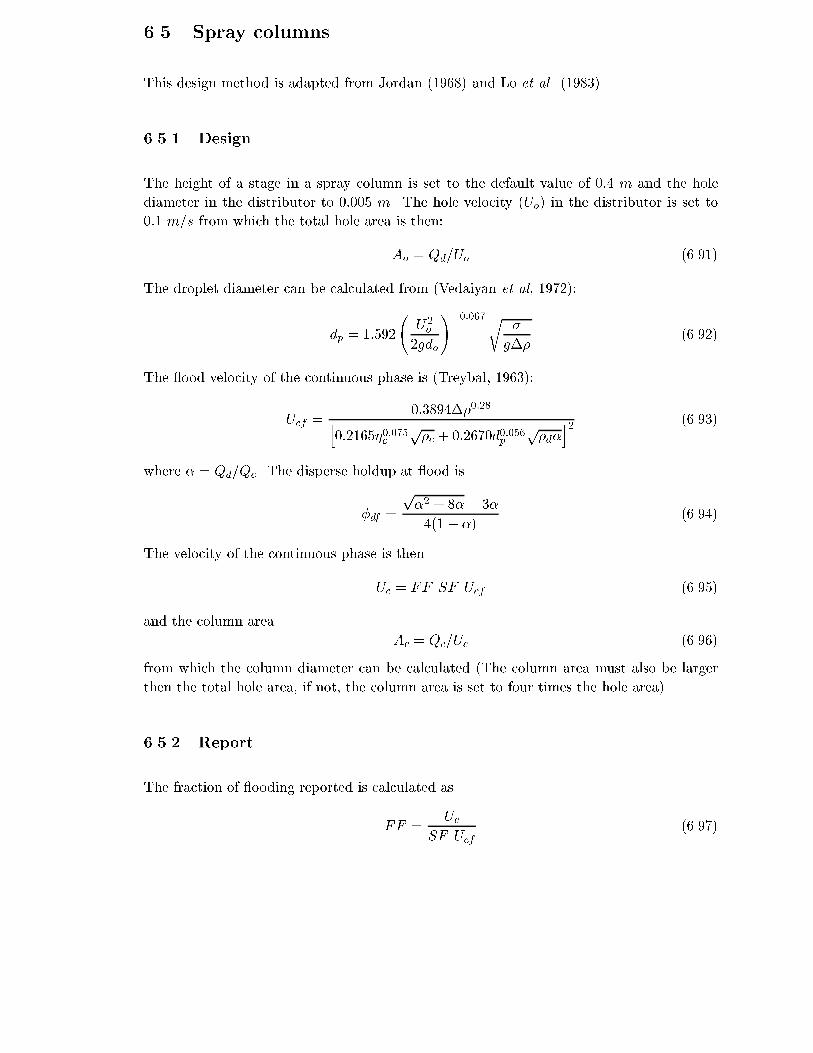
p y
6.5 Spray columns
This design method is adapted from Jordan (1968) and Lo et al. (1983).
6.5.1 Design
The height of a stage in a spray column is set to the default value of 0:4 m and the hole
diameter in the distributor to 0:005 m. The hole velocity (Uo) in the distributor is set to
0:1 m=s from which the total hole area is then:
Ao = Qd=Uo (6.91)
The droplet diameter can be calculated from (Vedaiyan et al, 1972):
dp = 1:592
U2o
2gdo
!�0:067r�
g��(6.92)
The ood velocity of the continuous phase is (Treybal, 1963):
Ucf =0:3894��0:28h
0:2165�0:075c
p�c + 0:2670d0:056p
p�d�
i2 (6.93)
where � = Qd=Qc. The disperse holdup at ood is
�df =
p�2 + 8�� 3�
4(1 � �)(6.94)
The velocity of the continuous phase is then
Uc = FF SF Ucf (6.95)
and the column area
Ac = Qc=Uc (6.96)
from which the column diameter can be calculated (The column area must also be larger
then the total hole area, if not, the column area is set to four times the hole area).
6.5.2 Report
The fraction of ooding reported is calculated as
FF =Uc
SF Ucf(6.97)

p q
where Ucf is computed as in the spray column design and Uc = Ac=Qc. No lower operating
limit is calculated. The dispersion coe�cient for the continuous phase is (Vermeulen et al.,
1966):Ec
VcH= 7:2
pUdDc (6.98)
Since the dispersion coe�cient for the disperse phase is unknown it is set equal to that for
the continuous phase.
6.5.3 Mass Transfer Coe�cients
The transition drop size below which droplets become stagnent is calculated from
P =�2c�
4
g�4c��(6.99)
dp;t = 7:25
r�
g��P 0:15(6.100)
The drop terminal velocity is (Satish et al., 1974):
Vt = 1:088
U2o
2gdo
!�0:082 ��g��
�2c
�1=4(6.101)
With the continous operating and ood velocities the fraction of ooding is calculated and
then the disperse phase holdup is
�d = FF �df (6.102)
and the slip velocity
Vs = (1� �d)Vt (6.103)
If the drops are stagnent (dp < dp;t) the disperse MTC is computed from
kd;ij = 18:9Dd;ij=dp (6.104)
else the Handlos-Baron correlation (1957) is used:
kd =0:00375Vs
(1 + �d=�c)(6.105)
For the continuous phase MTC we use (Ruby and Elgin, 1955)
kc = 0:725Re�0:43c Sc�0:58c (1� �d)Vs (6.106)
where
Rec = dpVs�c=�c (6.107)
Scc =�c
�cDc;ij
(6.108)
The interfacial area for mass transfer per unit of volume is
Ai =6�d
dp(6.109)

g
6.6 Modeling Back ow
The back ows in the column are computed from the dispersion coe�cients with:
�d =Ed
VdH� 0:5 (6.110)
�c =Ec
VcH� 0:5 (6.111)
where � is the fractional back ow ("entrainment") in the stage, and H is the stage height.
For spray columns (Perry, 198x):
Ec = 7:2pVdDc (6.112)
For packed columns:
logEd
VddF= 0:046
Vc
Vd+ 0:301 (6.113)
logEc
VcdF= 0:161
Vc
Vd+ 0:347 (6.114)
For a RDC:
Ec = 0:5HVc + 0:012RNH
�S
Dc
�(6.115)
Ed = FEc (6.116)
where F is calculated by
F =4:2105
D2c
�Vd
h
�3:3(6.117)
and must be larger or equal than one. Krishna uses:
Ec =0:5HUc
(1� �d)+ 0:012RNH
�S
Dc
�(6.118)
Ed =0:5HUd
�d
+ 0:024RNH
�S
Dc
�(6.119)
Symbol List
ap Packing area per unit volume (m2=m3)
as Static holdup area per unit volume (m2=m3)
Aa Total tray active area (m2)
Ad Downcomer area (m2)
Ai Interfacial area per unit volume (m2=m3)

p q
Ah Total tray hole area (m2)
An Netto tray area (m2), An = Aa +Ad
At Total tray area (m2)
Cd Drag coe�cient
D Binary di�usion coe�cient (m2=s)
Dc Column diameter (m)
de E�ective drop diameter (m) ?
dh Hole diameter (m)
dmin Minimum droplet diameter (m)
dp Sauter mean drop diameter (m)
Eo Eotvos number (��gdh=�)
f Free area ratio (Ah=Aa)
F Molar ow (kmol=s)
Fr Froude number (U2h=gdh)
FF Fraction of ooding
g, gc Gravitational constant, 9.81 (m=s2)
H RDC compartment height (m)
hc Height of coalesced layer (m)
h, hdrop Height of drop rising zone (m)
hstage Stage height for packed column (m)
k Binary mass transfer coe�cient (m=s)
Mw Molecular weight (kg=kmol)
N Rotation speed (rad=s)
Nu Nusselt number
Pe Peclet number
Pi Power input (?)
Q Volumetric ow (m3=s)
R Rotor diameter (m)
Re Reynolds number
S Inner stator diameter (m)
Sc Schmidt number
Sh Sherwood number
SF System derating factor
t Contact time (s)
ts Tray spacing (m)
Uc,Ud Continuous, disperse velocity (m=s)
Ucf Continuous phase super�cial velocity at ood (m=s)
Uh Hole diameter (m=s)
Vi Tray volume for interfacial mass transport (m3)
Vs Slip velocity (m=s)
V os Slip velocity at zero disperse phase holdup (m=s)
We Weber number (�dU2hdp=�)
Wl Weir length (m)

Greek:
� Phase ratio (Qd=Qc)
� Mass density (kg=m3)
�d Disperse phase holdup fraction
�ds Static disperse phase holdup fraction
� Interfacial tension (N=m)
� Liquid viscosity (Pa:s)
� Kinematic viscosity (�=�)
� Tortuosity
�
�
Subscripts:
c Continuous phase
d Disperse phase,
Downcomer
i Interface,
Component i
j Component j
References
F.H. Garner, M. Tayeban, Anal. Real Soc. Espan. Fis. Quim. (Madrid), Vol. B56 (1960)
pp. 479.
R.M. Gri�th, Chem. Eng. Sci., 12, 198 (1960).
A.E. Handlos, T. Baron, \Mass and Heat Transfer from Drops in Liquid-Liquid Extraction",
AIChE J., 3 (1957) pp. 127{136.
A.E. Handlos, T. Baron, AIChE J., 6, 145 (1957).
Hughmark, Ind. eng. Chem. Fundam., 6, 408 (1967).
D.G. Jordan, Chemical Process Development, Part 2, John Wiley, New York (1968).
W.J. Korchinsky, "Liquid-Liquid Extraction Column Modelling: Is the Forward Mixing
In uence Necessary?", Trans. I. Chem. E., Vol. 70, Part A, 333{345 (1992).
R. Krishna, S.M. Nanoti, A.N. Goswami, "Mass-Transfer E�ciency of Sieve Tray Extraction

p q
Columns", Ind. Eng. Chem. Res., Vol. 28 (1989) 642-644.
R. Krishna, Design of Liquid-Liquid Extraction Columns, University of Amsterdam (NL),
(1993).
R. Kronig, J.C. Brink, Appl. Sci Res., A2, 142 (1950).
A. Kumar, S. Hartland, "Prediction of Axial Mixing Coe�cients in Rotating Disc and
Asymmetric Rotating Disc Extraction Columns", Can. J. Chem. Eng, Vol. 70, 77{87
(1992).
A. Kumar, S. Hartland, "Prediction of drop size, dispersed-phase holdup, slip velocity, and
limiting throughputs in packed extraction columns", Trans. IChemE., 72, Part A, 89{104
(1994).
M. Lao et al., "A Nonequilibrium Stage Model of Multicomponent Separation Processes VI:
Simulation of Liquid-Liquid Extraction", Chem. Eng. Comm., 86, p73{89 (1989).
G.S. Laddha, T.E. Degaleesan, Transport Phenomena in Liquid Extraction, McGraw-Hill
(1978).
T.C. Lo, M.H.I. Baird, C. Hanson, Handbook of Solvent Extraction, John Wiley, NY (1983).
J.A. Rocha, J.L. Humphrey, J.R. Fair, "Mass transfer E�ciency of Sieve Tray Extractors",
Ind. Eng. Chem. Process Des. Dev., Vol. 25, No. 4 (1986) pp. 862{871.
P.N. Rowe, K.T. Claxton, J.B. Lewis, Transact. Inst. Chem. Eng., 43, T14 (1965).
P.M. Rose, R.C. Kinter, \Mass Transfer from Large Oscillating Drops", AIChE J., Vol. 12,
No. 3 (1966) pp. 530.
E.Y. Kung, R.B. Beckman, \Dispersed-Phase Holdup in a Rotating Disk Extraction Col-
umn", AIChE J., Vol. 7, No. 2 (1961) pp. 319-324.
A.M. Rozen, A.I. Bezzubova, Theor. found. Chem. Eng., 2, 715 (1968); translated from
Teor. Osnovy Khim. Tekh, 2, 850 (1968).
Ruby, Elgin, Chem. Eng. Prog., 51, Sump. Ser. 16, 17 (1955).
L. Satish, T.E. Dagaleesan, G.S. Laddha, Indian Chem. Eng., Vol. 16 (1974) pp. 36.
A.F. Seibert, J.R. Fair, "Hydrodynamics and Mass Transfer in Spray and Packed Liquid-
Liquid Extraction Columns", Ind. Eng. Chem. Res., 27, No.3, 470{481 (1988).
A.H.P. Skelland, R.M. Wellek, AIChE J., 10, 491 (1964).
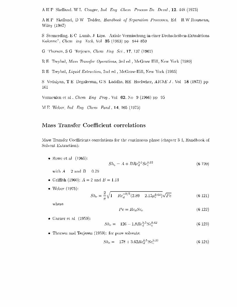
A.H.P. Skelland, W.L. Conger, Ind. Eng. Chem. Process De. Devel., 12, 448 (1973).
A.H.P. Skelland, D.W. Tedder, Handbook of Separation Processes, Ed. R.W.Rousseau,
Wiley (1987).
S. Stemerding, E.C. Lumb, J. Lips, \Axiale Vermischung in einer Drehscheiben-Extraktions
Kolonne", Chem. ing. Tech, Vol. 35 (1963) pp. 844{850.
G. Thorsen, S.G. Terjesen, Chem .Eng. Sci., 17, 137 (1962).
R.E. Treybal, Mass Transfer Operations, 3rd ed., McGraw-Hill, New York (1980)
R.E. Treybal, Liquid Extraction, 2nd ed., McGraw-Hill, New York (1963).
S. Vedaiyan, T.E. Degaleesan, G.S. Laddha, HE. Hoelscher, AIChE J., Vol. 18 (1972) pp.
161.
Vermeulen et al., Chem. Eng. Prog., Vol. 62, No. 9 (1966) pp. 95.
M.E. Weber, Ind. Eng. Chem. Fund., 14, 165 (1975).
Mass Transfer Coe�cient correlations
Mass Transfer Coe�cients correlations for the continuous phase (chapter 3.4, Handbook of
Solvent Extraction):
� Rowe et al. (1965):
Shc = A+BRe0:5d Sc0:33c (6.120)
with A = 2 and B = 0:79.
� Gri�th (1960); A = 2 and B = 1:13.
� Weber (1975):
Shc =2
�
q1�Re
�0=5d
(2:89 + 2:15�0:64r )pPe (6.121)
where
Pe = RedScc (6.122)
� Garner et al. (1959):
Shc = �126 + 1:8Re0:5d Sc0:42c (6.123)
� Thorsen and Terjesen (1959): for pure solvents:
Shc = �178 + 3:62Re0:5d Sc0:33c (6.124)

p q
Mass Transfer Coe�cients correlations for the disperse phase (chapter 3.4, Handbook of
Solvent Extraction):
� Kronig and Brink (1950):
Shd =kd�ddp
Dd
= 16:7 (6.125)
for Red < 50.
� Handlos and Baron (1957):
kd =0:00375Vs
1 + �d
�c
(6.126)
� Skelland and Wellek (1964):
Shd = 0:32Re0:68
�3�2cg�4c��
!0:10 4Dd;ijtc
d2d
!�0:14(6.127)
� Rozen and Bezzubova (1968):
a : Shd = 0:32Re0:63d Sc0:50d
�1 +
�d
�c
��0:5(6.128)
b : Shd = 7:5:10�5Re2:0d Sc0:56d
�1 +
�d
�c
��0:5(6.129)
for medium (a) and large (b) droplets.
where Reynolds, Schmidt, and Sherwood numbers are de�ned as:
Re =dp�Vs
�(6.130)
Sc =�
�Dij
(6.131)
Shij =kijdp
Dij
(6.132)
� =�
�(6.133)
Table 1 of chapter 10 in the Handbook of Solvent Extraction supplies us with three more
models for the drop rise zone. One for stagnant drops (Skelland and Conger, 1973):
kd = ��de
6t
���d
Md
�av
ln
1�
�D0:5vdt0:5
0:5de
!(6.134)
kc = 0:74
�Dvc
de
���c
Mc
�av
�deVs�c
�c
�0:5 � �c
�cDvc
�0:333(6.135)
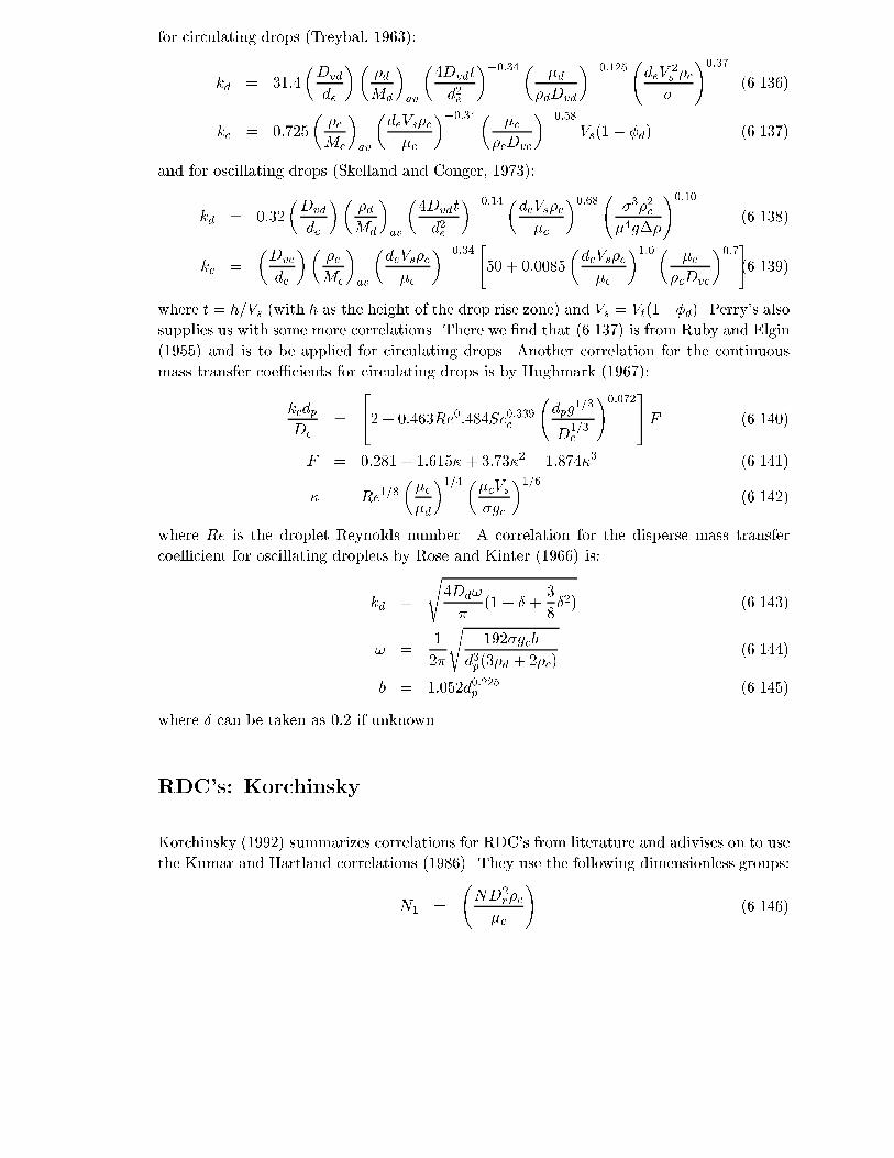
for circulating drops (Treybal, 1963):
kd = 31:4
�Dvd
de
���d
Md
�av
�4Dvdt
d2e
��0:34 � �d
�dDvd
��0:125 deV 2s �c
�
!0:37
(6.136)
kc = 0:725
��c
Mc
�av
�deVs�c
�c
��0:34 � �c
�cDvc
��0:58Vs(1� �d) (6.137)
and for oscillating drops (Skelland and Conger, 1973):
kd = 0:32
�Dvd
de
���d
Md
�av
�4Dvdt
d2e
��0:14 �deVs�c�c
�0:68 �3�2c�4g��
!0:10
(6.138)
kc =
�Dvc
de
���c
Mc
�av
�deVs�c
�c
��0:34 "50 + 0:0085
�deVs�c
�c
�1:0 � �c
�cDvc
�0:7#(6.139)
where t = h=Vs (with h as the height of the drop rise zone) and Vs = Vt(1��d). Perry's alsosupplies us with some more correlations. There we �nd that (6.137) is from Ruby and Elgin
(1955) and is to be applied for circulating drops. Another correlation for the continuous
mass transfer coe�cients for circulating drops is by Hughmark (1967):
kcdp
Dc
=
242 + 0:463Re0:484Sc0:339c
dpg
1=3
D1=3c
!0:07235F (6.140)
F = 0:281 + 1:615� + 3:73�2 � 1:874�3 (6.141)
� = Re1=8��c
�d
�1=4 ��cVs�gc
�1=6(6.142)
where Re is the droplet Reynolds number. A correlation for the disperse mass transfer
coe�cient for oscillating droplets by Rose and Kinter (1966) is:
kd =
s4Dd!
�(1 + � +
3
8�2) (6.143)
! =1
2�
s192�gcb
d3p(3�d + 2�c)(6.144)
b = 1:052d0:225p (6.145)
where � can be taken as 0:2 if unknown.
RDC's: Korchinsky
Korchinsky (1992) summarizes correlations for RDC's from literature and adivises on to use
the Kumar and Hartland correlations (1986). They use the following dimensionless groups:
N1 =
ND2
r�c
�c
!(6.146)
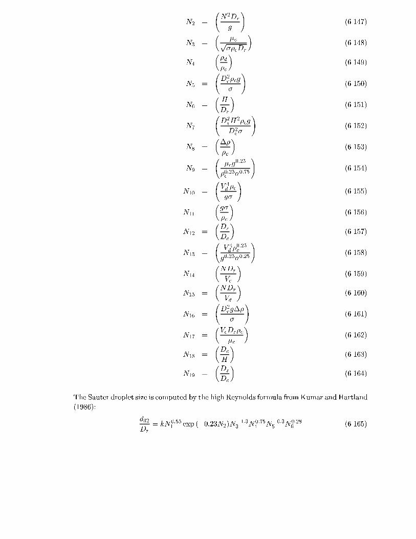
p q
N2 =
N2Dr
g
!(6.147)
N3 =
��cp��cDr
�(6.148)
N4 =
��d
�c
�(6.149)
N5 =
D2r�cg
�
!(6.150)
N6 =
�H
Dr
�(6.151)
N7 =
D2sH
2�cg
D2c�
!(6.152)
N8 =
���
�c
�(6.153)
N9 =
�cg
0:25
�0:25c �0:75
!(6.154)
N10 =
V 4d�c
g�
!(6.155)
N11 =
�g�
�c
�(6.156)
N12 =
�Dr
Dc
�(6.157)
N13 =
V 4d�0:25c
g0:25�0:25
!(6.158)
N14 =
�NDr
Vc
�(6.159)
N15 =
�NDr
Vd
�(6.160)
N16 =
D2rg��
�
!(6.161)
N17 =
�VcDr�c
�c
�(6.162)
N18 =
�Dc
H
�(6.163)
N19 =
�Ds
Dc
�(6.164)
The Sauter droplet size is computed by the high Reynolds formula fromKumar and Hartland
(1986):
d32
Dr
= kN0:551 exp (�0:23N2)N
�1:33 N0:75
4 N�0:35 N0:28
6 (6.165)

with 103k = 7:01 for no mass transfer. The Kumar and Hartland disperse holdup:
�d = [k1 + k2Nn12 ]Nn2
7 Nn38 Nn4
9 N0:2210
�1 +
Vc
Vd
�0:35(6.166)
where (using all data) k1 = 65:73, k2 = 74:20, n1 = 1:24, n2 = �0:34, n3 = �:049, andn4 = 0:53. The slip velocity is computed by
Vs = [k6 + k7 exp (�1:28N2)]N0:528 N0:25
11 N�0:459 N0:08
5 N1:036 N0:51
12 N0:2813 (6.167)
with (for all data) 102k6 = �5:11 and k7 = 0:20. the continuous phase dispersion coe�cient
is given by
Ec
VcH= 0:42 + 0:29
Vd
Vc+
�0:0126N14 +
13:38
3:18 +N14
�N�0:081 7N�0:16
12 N0:118 N
219 (6.168)
and the disperse phase coe�cients
Ed
VdH= 0:3
�Vc + Vd
Vd
�+ 9:37N15N
�0:6416 N�0:7
12 ��0:9d
(6.169)
Packed columns: Kumar and Hartland
Kumar and Hartland (1994) developed new correlations for the drop diameter, dispersed
phase holdup, slip velocity, and ooding velocities for packed extraction columns using a
large database. The Sauter mean droplet size is
dp = C1
"�wg
1=4�w
��1=4�3=4�d
#0:19r�
g��(6.170)
where C1 is 2:54, 2:24, or 3:13 for no mass transfer, transfer from c to d, and from d to c.
The dispersed phase holdup is
�d = C2e�1:11
���
�c
��0:50 24 1
ap
�2cg
�2c
!1=335�0:72 �
�d
�c
�0:10 "V d
��c
g�c
�1=3#1:03exp
"0:95Vc
��c
g�c
�1=3#
(6.171)
where C2 is 5:34, 6:16, or 3:76. The slip velocity is
Vslip = C3e�0:11
���
�c
�0:40 24 1
ap
�2cg
�2c
!1=3350:61 �
�d
�c
��0:10 � �c
g�c
��1=3(6.172)
where C3 is 0:24, 0:21, or 0:31. Or, as function of the dispersed phase holdup:
Vslip = C4e�0:17
���
�c
�0:41 24 1
ap
�2cg
�2c
!1=3350:59 �
�d
�c
��0:10 � �c
g�c
��1=3(1� �d) (6.173)

p q
where C4 is 0:30, 0:27, or 0:38. The ooding velocity is:
Vc;f (1 +pR)2
qap=g = �C1e
1:54
���
�d
�0:41 24 1
ap
�2cg
�2c
!1=3350:300
@ �cq���=ap
1A0:15
(6.174)
or
Vd;f
qap=g = �C1e
1:54
���
�d
�0:41 24 1
ap
�2cg
�2c
!1=3350:300
@ �cq���=ap
1A0:15
(6.175)
where � is 1:0 for continuous phase packing wetting and 1:29 for dispersed phase packing
wetting.

Chapter 7
Interface and Technical Issues
In this chapter we will brie y discuss ChemSep's internals. We discuss which programs
make up ChemSep and explain how they cooporate. All the supporting libraries and �les
are identi�ed and explained. More information on printing from within ChemSep and
other technical issues can be found in this chapter.
7.1 ChemSep Commandline Parameters
The following commandline parameters are optional when you start ChemSep by typing
cs at the commandline:
-sXX : where XX = 25, 28, 33, 35, 40, 43, or 50. This will set the number of lines on the
screen to the speci�ed number. Especially the 33 and 40 line modes are very handy.
The number of lines can also be set in the interface options.
-oFILE.CNF : loads options from FILE.CNF instead of CHEMSEP.CNF.
-kXXXX : stu�s all characters after the -k onto the keyboard bu�er as if they were typed in.
See the help for macro de�nitions for the handling of special keys.
-vx : disable the use of extended memory (XMS) for overlays.
-ve : disable the use of expanded memory (EMS) for overlays.
-vbXXXX : to set the bu�er size for overlay swapping to the hard disk where XXXX speci�es
the size in bytes.
Any other parameter will be handled as a Sep-�le, whichChemSep will try to load after the
introduction screen (the default "sep" extension does not need to be added). The interface
113
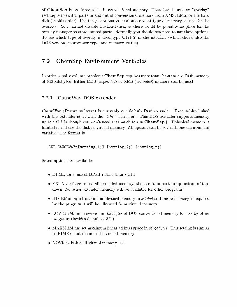
p
of ChemSep is too large to �t in conventional memory. Therefore, it uses an "overlay"
technique to switch parts in and out of conventional memory from XMS, EMS, or the hard
disk (in this order). Use the /v options to manipulate what type of memory is used for the
overlays. You can not disable the hard disk, as there would be possibly no place for the
overlay manager to store unused parts. Normally you should not need to use these options.
To see which type of overlay is used type Ctrl-Y in the interface (which shows also the
DOS version, coprocessor type, and memory status).
7.2 ChemSep Environment Variables
In order to solve column problemsChemSep requires more than the standard DOS memory
of 640 kilobytes. Either EMS (expanded) or XMS (extended) memory can be used.
7.2.1 CauseWay DOS extender
CauseWay (Devore software) is currently our default DOS extender. Executables linked
with this extender start with the "CW" characters. This DOS extender supports memory
up to 4 GB (although you won't need that much to run ChemSep!). If physical memory is
limited it will use the disk as virtual memory. All options can be set with one environment
variable. The format is
SET CAUSEWAY=[setting_1;] [setting_2;] [setting_n;]
Seven options are available:
� DPMI; force use of DPMI rather than VCPI
� EXTALL; force to use all extended memory, allocate from bottom-up instead of top-
down. No other extender memory will be available for other programs
� HIMEM:nnn; set maximum physical memory in kilobytes. If more memory is required
by the program it will be allocated from virtual memory
� LOWMEM:nnn; reserve nnn kilobytes of DOS conventional memory for use by other
programs (besides default of 32k)
� MAXMEM:nn; set maximum linear address space inMegabytes. This setting is similar
to HIMEM but includes the virtual memory
� NOVM; disable all virtual memory use

p
� SWAP:path; set swap �le path. This path takes precedence for choosing the location of
a swap �le over the regular TEMP and TMP environment variables that are normally
used for these �les. Useful to specify a path on a local rather than a network drive
7.2.2 Rational
The DOS Rational extender was our previous choice of DOS extender. Executables linked
with this extender start with the "4G" characters. The DOS extender selects EMS and
then XMS. You can force the DOS extender to use XMS above EMS by specifying it to use
a block of memory larger than the available EMS. For example, the environment variable
dos16m=:4m requests a block of memory of 4 MB (use the DOS set command to specify
environment variables). If there is more than 4 MB of EMS available the DOS extender will
use EMS, otherwise it will try to use 4 MB of XMS. If the physical memory in your machine
does not allow you to run a large problem you can use virtual memory which is swapped to
your hard disk by using the following environment variable setting: dos4gvm=deleteswap
which allows up to 16 MB of virtual memory and deletes the swap �le after the run is
completed. The virtual memory is swapped to the DOS4GVM.SWP �le which is placed in
the root directory of the current drive.
7.2.3 SVGA drivers
In case the automatic selection of the Super VGA drivers XVGA16 and XVGA256 select a wrong
video chipset, you can set the CHIPSET environment variable to change the detection test.
For example SET CHIPSET=VESA,CRRS will set the CHIPSET environment variable so that
the Super VGA driver will �rst test for VESA, if this fails for Cirrus, and if this also fails
it will use a generic VGA mode. The chipset codes are (in the standard detection order):
EVRX (Everex), CMPQ (Compaq), V7 (Video 7), C&T (Chips & Tech), CRRS (Cirrus),
ATI, TSNG (Tseng), OAK, (Oak Technologies), GNOA (Genoa), TRID (Trident), PRDS
(Paradise), NCR, AHED (Ahead Systems), S2, VESA.
7.2.4 Printer drivers
The printer drivers also can make use of extended/expanded memory for generating tempo-
rary raster �les for the printouts. At the moment, no options can be set through environment
variables for the memory use of these drivers.

p
7.3 ChemSep's Programs
ChemSep is not one program but is split into several executables and associated data
�les. Before we can explain in detail how ChemSep uses the programs lets �rst see what
program names are present in the executables directory and what they do:
� CS.EXE: the driver for ChemSep
� CS2.EXE: ChemSep interface
� CSW.EXE: the solve driver
� (CW-)COL2.EXE: COLumn simulator
� (CW-)NEQ2.EXE: NonEQuilibrium column simulator
� CP.EXE: the driver for ChemProp
� CP1.EXE: ChemProp interface
� CL.EXE: ChemLib interface
The drivers acts as the glue between all the interfaces and simulators. It also gives us exi-
bility in the way we run our programs and hides details from the average user. ChemSep
and ChemProp are normally started by running their drivers: CS.EXE and CP.EXE, re-
spectively. However, both ChemProp and ChemLib can be run from within the ChemSep
interface through menu options under the input menu.
The "CW-" in front of the calculation programs denotes the DOS extender type that is
linked to the executables. CauseWay executables include the DOS extender, the Ratio-
nal DOS-Extender uses a separate �le (DOS4GW.EXE). The executables often need at
least two MegaByte of Extended memory in order to run. They also require a 386-based
system (minimum) to run. The di�erent DOS extender executables can be selected un-
der Options/DOS-Extender. Check this setting when you get error messages stating that
executables with the "CW-" or "4G-" are not found. CauseWay is currently our default.
As we support the simulators on other platforms as well, they must also run without the
ChemSep interface. That is why we store all information (in- and output) in the problem
�les, with the .SEP extension. As the simulator must know what problem �le to run it
checks for the existance of the CHEMSEP.FIL �le. If it exists, it will read this name
from this �le. If the �le doesn't exist or no CHEMSEP.FIL �le was found in the current
directory, the simulator will prompt you for a SEP �le. DOS and Windows executables
of the simulators also allow speci�cation of the SEP �le on the commandline, making the
CHEMSEP.FIL unnecessary.
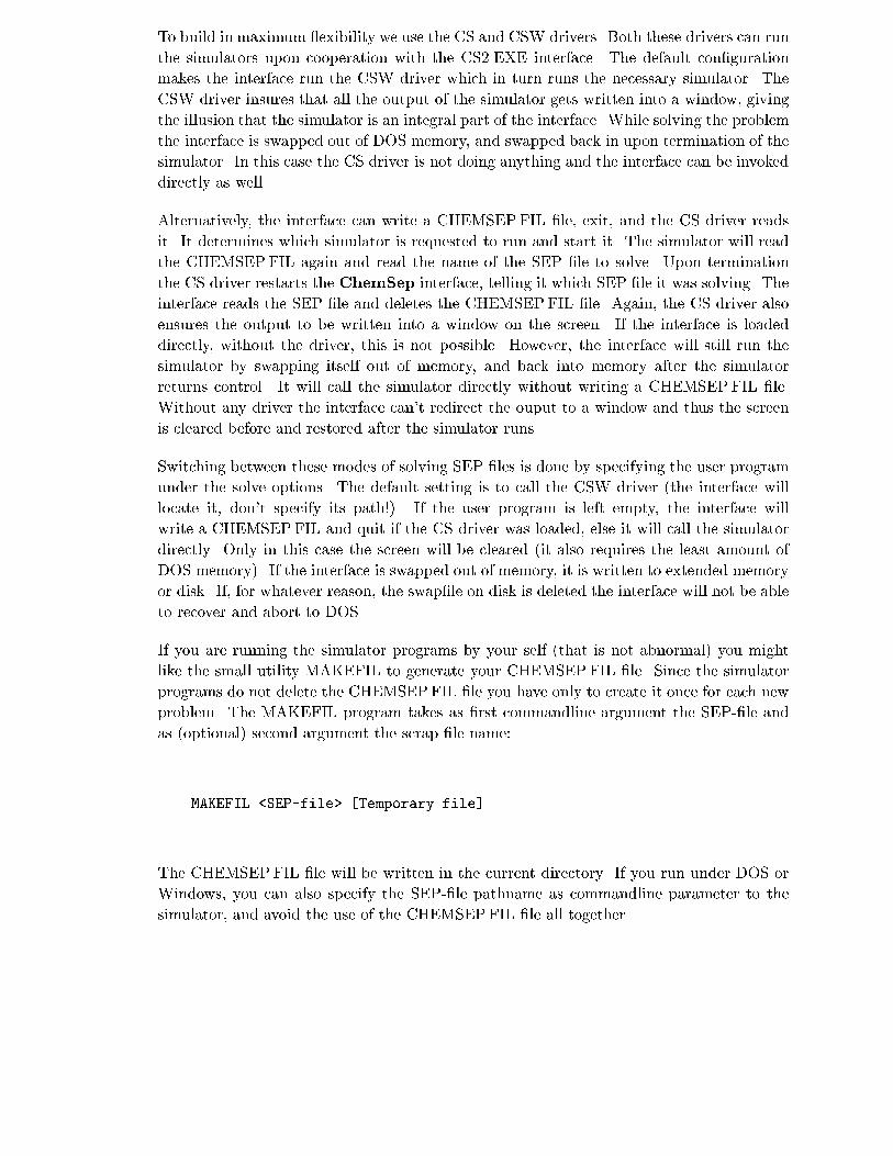
p g
To build in maximum exibility we use the CS and CSW drivers. Both these drivers can run
the simulators upon cooperation with the CS2.EXE interface. The default con�guration
makes the interface run the CSW driver which in turn runs the necessary simulator. The
CSW driver insures that all the output of the simulator gets written into a window, giving
the illusion that the simulator is an integral part of the interface. While solving the problem
the interface is swapped out of DOS memory, and swapped back in upon termination of the
simulator. In this case the CS driver is not doing anything and the interface can be invoked
directly as well.
Alternatively, the interface can write a CHEMSEP.FIL �le, exit, and the CS driver reads
it. It determines which simulator is requested to run and start it. The simulator will read
the CHEMSEP.FIL again and read the name of the SEP �le to solve. Upon termination
the CS driver restarts the ChemSep interface, telling it which SEP �le it was solving. The
interface reads the SEP �le and deletes the CHEMSEP.FIL �le. Again, the CS driver also
ensures the output to be written into a window on the screen. If the interface is loaded
directly, without the driver, this is not possible. However, the interface will still run the
simulator by swapping itself out of memory, and back into memory after the simulator
returns control. It will call the simulator directly without writing a CHEMSEP.FIL �le.
Without any driver the interface can't redirect the ouput to a window and thus the screen
is cleared before and restored after the simulator runs.
Switching between these modes of solving SEP �les is done by specifying the user program
under the solve options. The default setting is to call the CSW driver (the interface will
locate it, don't specify its path!). If the user program is left empty, the interface will
write a CHEMSEP.FIL and quit if the CS driver was loaded, else it will call the simulator
directly. Only in this case the screen will be cleared (it also requires the least amount of
DOS memory). If the interface is swapped out of memory, it is written to extended memory
or disk. If, for whatever reason, the swap�le on disk is deleted the interface will not be able
to recover and abort to DOS.
If you are running the simulator programs by your self (that is not abnormal) you might
like the small utility MAKEFIL to generate your CHEMSEP.FIL �le. Since the simulator
programs do not delete the CHEMSEP.FIL �le you have only to create it once for each new
problem. The MAKEFIL program takes as �rst commandline argument the SEP-�le and
as (optional) second argument the scrap �le name:
MAKEFIL <SEP-file> [Temporary file]
The CHEMSEP.FIL �le will be written in the current directory. If you run under DOS or
Windows, you can also specify the SEP-�le pathname as commandline parameter to the
simulator, and avoid the use of the CHEMSEP.FIL �le all together.

p
7.4 Running ChemSep - Advanced Use
As noted in the previous section, ChemSep has separate programs for the calculations and
interfacing with the user. In order for the Driver to know what is going on, the interface
saves information in the CHEMSEP.FIL such as the name of the SEP-�le, the program
to run, the temporary scrap �le name, the user program, the run window coordinates and
color as well as the starttime.
In order to make ChemSep as versatile as possible, we implemented the User Program
entry under the "User program" option in the "Solve Options" menu. If you want to run
your own program you can enter its full path and name (with the extension!) there and
that program will be run no matter what kind of operation is selected. In order for a user
program to have access to the SEP-�le, the interface provides the user program with its
name as the second commandline parameter. In case it also wants to use the temporary
�le, that is supplied as the third parameter. Running a user program will clear the screen
before it starts executing the user program.
It is logical to suppose that the user just might want to run several programs or his own
program(s) before/after calling ChemSep's original calulation programs. To allow this you
can use a batch �le as the user program (use complete path, name and extension !). Look
up in your DOS manual how to make batch �les. In order to run the original calculations
program we provide it to the batch �le as the �rst commandline parameter and the SEP-�le
as the second. Even running the user program, the Interface generates a CHEMSEP.FIL
�le to be read by the calculation program. Here's an example of such a batch �le that will
type the problem SEP-�le �rst before running (note how the parameters are accessed with
%1 and %2):
@Echo off
Rem -----------------------------------------------------------
Rem Echo is set off to avoid to show this batch file is running
Rem use the "@" to suppress echoing of commands to the screen
Rem -----------------------------------------------------------
Rem Type the SEP-file:
Rem ------------------
Type %2
Rem Pause for the user to strike a key:
Rem -----------------------------------
Pause
Rem Run the appropriate ChemSep calculation:
Rem ---------------------------------------
%1
Rem Done!
p
Of course you can leave out all the Rem(arks) if you type this batch �le but it is a good
habit to document your code ! You might create a complete set of batch �les for di�erent
problems. Programs that might be run after the calculation might be cost estimation or
design (in case of equilibrium simulation) programs. Using command line parameters (or
the CHEMSEP.FIL �le) your program might append its results to the SEP-�le, so all results
will be collected in there. Here is an example of a batch �le that will automatically run
ChemProp to generate physical property information in the sep-�le:
@Echo off
echo Running ChemSep with physical property information generation
rem Run executable
%1
rem Run ChemProp to generate physical property information
c:\chemsep\bin\cp /c %2
rem Done!
The ultimate freedom is allowed by typing "DODOS" as User Program in the Interface. The
driver will automatically locate DOS and run it. All Dos commands will be available to you.
The only way to access the SEP-�le and other information is to read the CHEMSEP.FIL
�le. When you are ready to go back to the Interface you type "EXIT" and press Enter.
By allowing you to shell to DOS or run batch �les from within ChemSep we have created
the maximum exibility. Although ChemSep takes a lot of e�ort to prevent your system
or ChemSep from crashing, it is possible to do so, using batch �les or the DOS shell.
Avoid deleting crucial �les (such as executable �les), or changing system parameters while
the ChemSep-Driver is loaded. Do not load any TSR (Terminate and Stay Resident)
programs or device drivers, since these programs will be removed from memory after the
Driver takes over again. However, the interrupt to trigger these programs usually remains
active. Changing directories is allowed, but remember the current CHEMSEP.FIL is written
in the current directory ! The driver will change the directory back to what it started
running from, when returning to the Interface. If you want to change the current directory
use the Directory option in the File menu ! Do not load ChemSep again by invoking the
driver, as multiple copies will be loaded into memory.
7.5 ChemSep Libraries and Other Files
A number of libraries has been added to the ChemSep package. We can divide the data
libraries into the following groups:
� Pure Component Data (*.PCD)

p
� Interaction Parameter Data (*.IPD)
� Pure component LIBraries (*.LIB)
� Group Component Data (*.GCD)
� Internals Layout Data (*.ILD)
� Packing Data (CHEMSEP.*PD)
� Various ChemSep �les (CHEMSEP.*)
The Pure Component Data (PCD) �les contain the information of pure components like
molecular weight, critical temperature, acentric factor, vapour pressure correlation con-
stants, UNIFAC group ID's and number of groups etc. To access this data we have developed
ChemLib which is a completely menu driven data manager - very similar to ChemSep, in
fact - that will allow you to search PCD-�le(s) and select component data records to edit.
It can also move components from one PCD-�le to another, or to text �les. ChemSepv3.5
and higher can also use components from text �les instead of PCD �les. We prefer the
faster (to search) binary PCD format for distribution, however, component data informa-
tion in text format can have additional information as long as you append this information
after the regular component's data items in the text �le (ChemSepand ChemLibwill stop
reading after the �xed set of items and look for the start of the next component). The
components ID numbers (Library Index) are based on the system developed at Penn State
University and adopted by DIPPR.
The Interaction Parameter Data (IPD) �les are ASCII text �les with the interaction param-
eters for activity coe�cient models and equations of state. Currently we have the following
IPD �les:
� NRTL.IPD
� UNIQUAC.IPD
� UNIQUACP.IPD (UNIQUAC Q' activity coe�cient model)
� PR.IPD (Peng-Robinson EOS)
� SRK.IPD (Soave-Redlich-Kwong EOS)
� HAYDENO.IPD (Hayden O'Connell Virial EOS)
All these �les are in plain text format �le so the user can extend the data �les (it is probably
better to backup the original �les or to use a new name for the extended �les). Edit these
�les with any ASCII editor, or the built-in editor in ChemSep. The data in these �les

p
comes after the line with the [IPD] keyword. The next line contains the �le-comment after
the "=", which will be used as a header in the interface. Next comes a line (only for activity
coe�cient models) with the interaction parameters units. Next comes the data, one line per
binary pair. The �rst two numbers are the component library indices, then the interaction
parameters. Appended text is optional but will also be displayed. As an example we include
the �rst relevant lines of the NRTL.IPD �le:
[IPD]
Comment=DECHEMA NRTL data @ 1atm.
Units=cal/mol
#
1101 1921 -189.0469 792.8020 0.2999 Methanol/Water p61 1/1a
Lines starting with a "#" are comment lines which may appear anywhere. Since the inter-
face will only start reading the �le from the [IPD] keyword on, you can start the �le with
some text describing where the data was obtained and remarks on who/when/how changed
the �le. Most of the IPD �les contain information from the DECHEMA series, a very ex-
tensive collection of interaction parameters. The Hayden O'Connell virial parameters are
from Prausnitz et al. (1980).
Polynomial K-value and enthalpy correlation coe�cients as well as extended Antoine coef-
�cients are stored as component LIBraries (LIB �les), which are ASCII �les as well. The
default LIB �les are
� EANTOINE.LIB (Extended Antoine)
� H-POLY.LIB (Example polynomial enthalpy coe�cients
� K-POLY.LIB (Example polynomial K-value coe�cients
Here the interface starts reading the �le after the [LIB] keyword. Again a comment is read
from the next line (after the "=") and then the data starts with a line for each component
(�rst the library index followed by the coe�cients). For example the extended Antoine �le
(with data from Prausnitz et al., 1980) starts like:
[LIB]
Comment=Extended Antoine Prausnitz et al.
#
# ID A B C D E F G
902 3.15799e+01 -3.2848e+2 0. 0. -2.5980e+0 0. 2.0 Hydrogen
p
Group Component Data (GCD) �les are binary �les containing data for group contribu-
tion method such as UNIFAC or ASOG. Currently only UNIFAC �les are present (UNI-
FACRQ.GCD, UNIFACVL.GCD and UNIFACLL.GCD) for Vapour-Liquid and Liquid-
Liquid systems. These �les need not be changed, unless for example the UNIFAC group
tables have changed. Several GCD-�les are used for the estimation of pure component data
in ChemLib and UserPcd.
Internal layout data (ILD) �les are text �les which store tray or packing layouts for use
by the nonequilibrium model. This way a speci�c design can be saved and reloaded upon
demand.
Packing Data (CHEMSEP.*PD) �les contain many physical and model parameters for var-
ious random and structured packings. They are text �les that might be modi�ed by the
user with an ASCII editor, though there is one restriction, namely that the �rst line should
not be changed! A shortened version of the structured packing data �le CHEMSEP.SPD is
shown below.
# CHEMSEP SPD Structured Packing Data
#
# Type (Name): Specific Equiv. Channel Packing Void ...
# packing diam. flow factor: fract: ...
# surface: angle:
!----------------------
Koch Flexipac 1 M 558/m 0.00897m 45 98/m 0.91 ...
Koch Flexipac 2 SS 223/m 0.01796m 45 43/m 0.95 ...
Koch Flexipac 3 M 135/m 0.03592m 45 26/m 0.96 ...
Koch Flexipac 4 M 69/m 0.07183m 45 20/m 0.98 ...
@----------------------
Glitsch Gempak 1A M 131/m 0.03592m 45 30/m * ...
Glitsch Gempak 2A SS 223/m 0.01796m 45 52/m 0.95 ...
Glitsch Gempak 2AT SS 223/m 0.01796m 45 * 0.96 ...
Glitsch Gempak 3A M 394/m 0.01346m 45 69/m * ...
Glitsch Gempak 4A M 525/m 0.00897m 45 105/m * ...
Lines starting with "#" are comment lines and are ignored (except for the �rst line). A
line starting with "!" is used to set the length of the packing type identi�ers which is set
equal to the length of that line. Lines starting with an "@" will insert a separator in the list
with packings and blank lines will be ignored. As you can see units may be added as long
as there is no space between the number and the unitstring (otherwise errors will occur in
reading this �le!).
Miscellaneous ChemSep �les include:
p
� CHEMSEP.UDF: Units De�nition File
� CHEMSEP.SYN: SYNonyms �le
� CHEMSEP.HLP: HeLP �le
� CHEMSEP.TXT: The ChemSep book in ASCII TeXT format
� CHEMSEP.CNF: the default CoNFiguration �le
� CHEMSEP.SCR: the additional introduction SCReen(s)
The CHEMSEP.UDF �le contains the de�nitions for the units and the unit conversions in
ChemSep. The �rst line must have the number of following lines with on each a unit
de�nition. Such a unit de�nition consists of 15 characters (from column 1) with the unit
abreviation (take care, these are case sensitive !) followed by 15 characters (from column
16) with the full unit name (not case sensitive). Then, from column 31 the o�set-factor (fo)
and multiplication factor (fm) come and �nally the reference unit. The conversion is done
according the following formula:
Number (in Reference units) = fm * ( Number (in Units) - fo )
For example 22C = 1:0(22 � �273:15) = 295:15K. You can inspect ASCII text �les with
ChemSep's �le viewer (F7) or make simple modi�cations with edit-�le. However, we
strongly suggest you do not change the original data �les that come with ChemSep. We
carefully selected and typed the data into these �les and other users might use your changed
data and obtain erroneous results. We urge you �rst to copy the �le to another name
before you change or add anything in these �les. Errors in the unit conversion can be very
frustrating so it is good to check some results if you have changed or added a unit de�nition.
To encourage you to do so we made CHEMSEP.UDF a read-only �le !
The CHEMSEP.SYN is a �le containing synonyms for over 1000 compounds. While search-
ing for a special component name you can use synonyms if you have selected to do so in
the options interface spreadsheet. You must select this �le as your synonyms �le. The
synonym search does not work while typing in a searchlist for a synonyms name. You will
have to issue a search under the synonyms name ! The synonyms �le is an ASCII �le you
can modify to your needs.
The CHEMSEP.HLP �le contains the information to provide you with help when you press
(F1) for help. It is a binary �le that can not be changed. It is generated with the MAKE-
HELP utility from help source (HSR) �les. This utility and the source �les are not part of
the ChemSep distribution. If you �nd errors or shortcomings in the help please notify the
authors.

p
The CHEMSEP.TXT �le contains the ASCII text of this book. Normally ChemSep will
be con�gured with function key (F9) assigned to automatically load this �le. There are
also other formats available on our ftp-site (see Author information). The ASCII version is
somewhat limited in available characters, sub- or superscripts, and equations.
The CHEMSEP.CNF �le is used to store the default con�guration, such as the macro de�-
nitions, directory structure, selected video and printer devices, and solve options. CHEM-
SEP.CNF is the default con�guration �le which will be loaded upon startup of the interface.
If none is found in the current directory, the �le supplied in the original distribution is used.
This allows one to have multiple CHEMSEP.CNF �les in di�erent directories, which auto-
matically con�gure the interface to (a) speci�c problem(s).
Finally, the CHEMSEP.SCR �le contains the additional introduction screen(s) that are
shown on startup of the program. These are used to stipulate conditions of the use of the
program, but could can be adapted to suit the users needs (for example if ChemSep is
installed on a network, the operator can place important notes here). If the �le contains
more lines than can be shown on the screen, the user will have to press <Enter> multiple
times to go through the various screens sequentially.
7.6 The SEP-�le format
The SEP-�les are written in a format which is readible by a human as well as by the
calculation program. However, there are some strict rules ! The SEP-�le is constructed using
delimiters in square brackets: []. The order of the delimeters is not directly of importance
(although ordering delimiters enhances the speed of reading a SEP-�le). The sections
under the delimiters are ordered and have a �xed format. Usually they consist of lines
with a selected value and a comment. ChemSep uses two major sections: the INPUT and
RESULTS sections. The INPUT starts with the delimiter [ChemSep] and ends with [End
of Input]. The Results starts with [Results] and ends with [End of Results]. Within these
sections there are sub sections. Note that a "*" denotes that the value is not yet set by
the user. In some cases the Interface might create cryptic "* *" lines where the �rst star
denotes the (not yet known) value of a selector and the second the description of the (not
yet) selected item.
Remember that normally the Interface will not read any comments you have added yourself
to the SEP-�le and thus, not save them again when saving from within the Interface. To
overcome this problem we have added the [User-Data] and [End User-Data] delimiters.
When loading a SEP-�le it is the last section that is looked for. If found, it is read into a
bu�er and written back to the �le if saved again. Note that the delimiters each have to be
on a separate line. You can use this data block to save information about the problem or
to store parameters for your own programs that process SEP-�les. You can edit User Data
within the interface of ChemSep under the Solve Options (F6). The following keywords
are used to switch several hidden features (with explanation in "()"):
[D-Models]
Diffusivity model (0=Maxwell-Stefan, 1=Effective)
Liquid MS-diffusivity model (0=Kooijman-Taylor, 1=Wesselingh-Krishna)
[No user interaction] (if present the user is not asked for
more iterations if maximum number has
been reached, but the program exits)
[Sensitivity] (sensitivity factors)
Vapour/Light-liquid Mass Transfer Coefficient
Liquid/Heavy-liquid Mass Transfer Coefficient
Interfacial Area
For a column problem the INPUT subsections are:
[CHEMSEP]
Version number and SEP file name
[Paths]
Current directories
[Units]
Current set of units
[Components]
Number of components, for each component library offset (in the PCD file),
Index, Name, and PCD-library filename
[Operation]
Operation type and kind, condenser and reboiler types, number of stages,
feeds, sidestreams, and pumparounds.
[Properties]
Property selections:
[Thermodynamics]
K model, Activity coefficient, Wilson model, UNIQUAC model, Equation of
State, Cubic EOS, Virial EOS, Vapour pressure models

p
[Enthalpy]
Enthalpy model
[Physical Properties]
Physical Properties model selections
[Property Data]
Pure component data or interaction parameters if required
[Specifications]
Specifications:
[Heaters/Coolers]
Number and stage with duty, if specified.
[Sections]
Number and for each section: section number, begin and end stages, model
selections, and tray/packing layout data.
[Efficiencies]
default efficiency, number of exceptions and stage with value, if
specified.
[Pressures]
Type of pressure specification, condenser, top, bottom pressures, pressure
drop.
[Feeds]
Number and for each feed: feed state, stage, temperature, pressure, vapour
fraction, number of componentflows, molar component flows.
[SideStreams]
Number and for each sidestream: stage, phase, specification type and value.
[Condenser]
Specification type and value(s) if present
[Reboiler]
Specification type and value(s) if present
[Solve options]
Initialization type, solving method, damping factor (if present), accuracy,

maximum number of iterations, and print options.
[Programs]
Temporary file, and user program
[User-Data]
Here the user data text is written.
[End User-Data]
[End of Input]
For an equilibrium column the [Sections] subsection will be absent, for a nonequilibrium
model the [E�ciencies] subsection is not needed. For a ash a di�erent set of speci�cations
is present consisting of the [Feeds] subsection and a [Flash] specifcation subsection where
ash type and specifactions are made. The RESULTS section for a nonequilibrium problem
looks like:
[Results]
[Profiles]
[Temperatures]
[Vapour phase compositions]
[Liquid phase compositions]
[Interface vapour mole fractions]
[Interface liquid mole fractions]
[Murphree efficiencies]
[Mass transfer rates]
[Condenser Heat Duty]
[Reboiler Heat Duty]
[K-values]
[Feed streams]
[Top product]
[Bottom product]
[Sidestreams]
[Designed Sections]
[Operating Limits]
[End of Results]
For equilibrium problems the Interface mole fractions, Murphree e�ciencies, mass transfer
rates, designed sections, and operating limits will be missing from the above list.
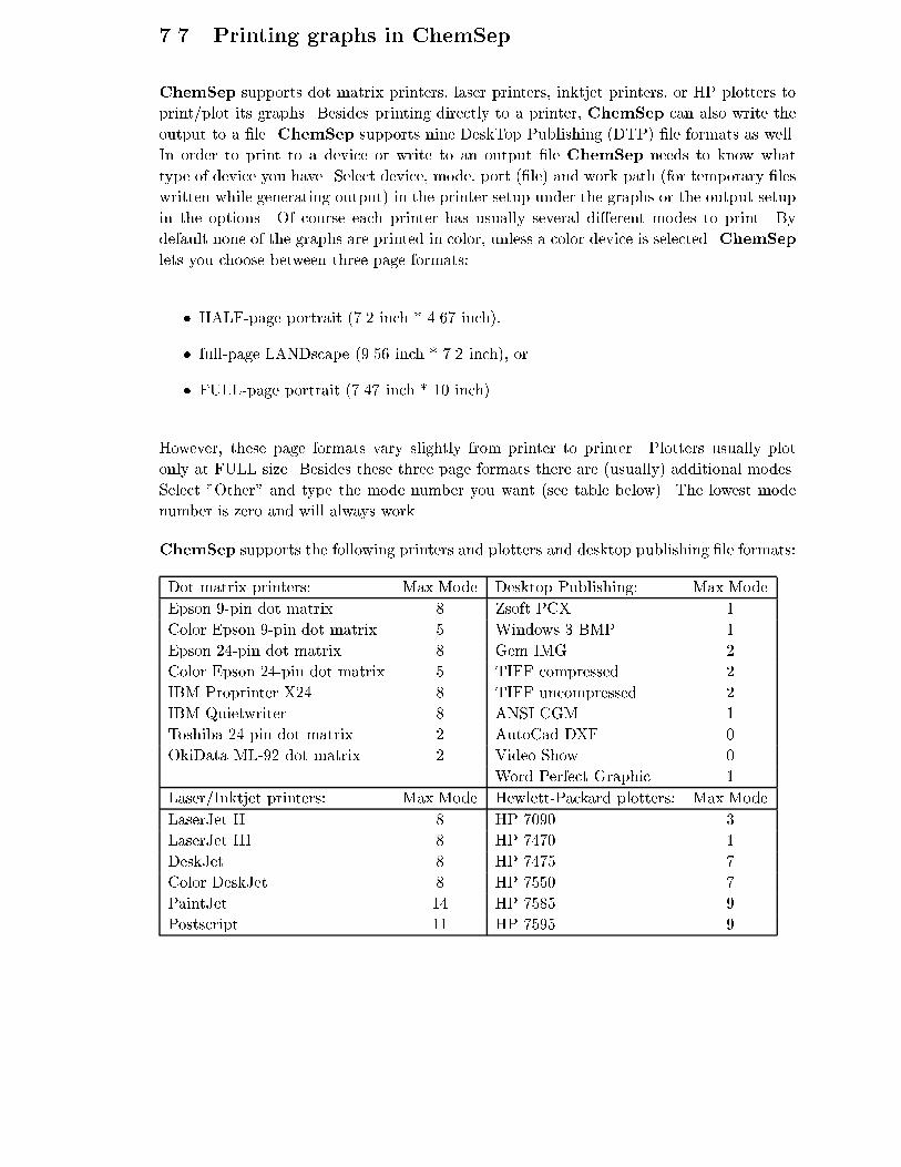
p
7.7 Printing graphs in ChemSep
ChemSep supports dot matrix printers, laser printers, inktjet printers, or HP plotters to
print/plot its graphs. Besides printing directly to a printer, ChemSep can also write the
output to a �le. ChemSep supports nine DeskTop Publishing (DTP) �le formats as well.
In order to print to a device or write to an output �le ChemSep needs to know what
type of device you have. Select device, mode, port (�le) and work path (for temporary �les
written while generating output) in the printer setup under the graphs or the output setup
in the options. Of course each printer has usually several di�erent modes to print. By
default none of the graphs are printed in color, unless a color device is selected. ChemSep
lets you choose between three page formats:
� HALF-page portrait (7.2 inch * 4.67 inch),
� full-page LANDscape (9.56 inch * 7.2 inch), or
� FULL-page portrait (7.47 inch * 10 inch).
However, these page formats vary slightly from printer to printer. Plotters usually plot
only at FULL size. Besides these three page formats there are (usually) additional modes.
Select "Other" and type the mode number you want (see table below). The lowest mode
number is zero and will always work.
ChemSep supports the following printers and plotters and desktop publishing �le formats:
Dot matrix printers: Max.Mode Desktop Publishing: Max.Mode
Epson 9-pin dot matrix 8 Zsoft PCX 1
Color Epson 9-pin dot matrix 5 Windows 3 BMP 1
Epson 24-pin dot matrix 8 Gem IMG 2
Color Epson 24-pin dot matrix 5 TIFF compressed 2
IBM Proprinter X24 8 TIFF uncompressed 2
IBM Quietwriter 8 ANSI CGM 1
Toshiba 24-pin dot matrix 2 AutoCad DXF 0
OkiData ML-92 dot matrix 2 Video Show 0
Word Perfect Graphic 1
Laser/Inktjet printers: Max.Mode Hewlett-Packard plotters: Max.Mode
LaserJet II 8 HP 7090 3
LaserJet III 8 HP 7470 1
DeskJet 8 HP 7475 7
Color DeskJet 8 HP 7550 7
PaintJet 14 HP 7585 9
Postscript 11 HP 7595 9

Table 7.1: Interface Assigned Types
Operation InternalType ModelType
Vapor-Liquid (VL) Discrete (DIT) Mass transfer coe�cient (MTC)
Liquid-Liquid (LL) Continuous (CIT) Pressure drop (PD)
Vapor ow (VF)
Liquid ow (LF)
Entrainment (Entr)
Holdup (Hold)
Light liquid ow (LLF)
Heavy liquid ow (HLF)
Backmixing (Back)
7.8 Model De�nition and Selection
ChemSep reads a de�nitions �le (CHEMSEP.DEF) at startup, where models for the mass
transfer coe�cients, pressure drop, ow models, entrainment, and holdup are de�ned. This
alleviates us from adapting the ChemSep interface upon any addition or modi�cation of a
model. In case no de�nitions �le is found, the nonequilibrium part of ChemSep is disabled.
The de�nitions �le must start with "[ChemSep De�nitions]" followed by a Version �eld (like
"Version=1.00"). Lines that start with "#" are comment lines. Five di�erent de�nitions
are in the �le: [InternalType], [Operation], [ModelType], [Internal], and [Model]. Each of
these has the following �elds: ID, Name, and Short, for example:
[Operation]
ID=1
Name=Vapor-Liquid
Short=VL
The �ve di�erent types of de�nitions may be mixed throughout the de�nitions �le. The
[Internal] de�nitions also contain the �elds: Type, Operation, Models, and Parameters.
The [Model] de�nitions also contain the �elds: Type, Operation, Internals, and Parameters.
Short �elds are optional, and have a maximum length of ten characters, used for displaying
selected models etc. ID �elds associate a unique number to the de�nition. Only for the
internal and model de�nitions non-unique numbers are allowed. When the interface reads
the de�nitions �le it uses the Short descriptions to assign the ID's for the Operations,
InternalTypes and ModelTypes, see Table 7.1 (the Short descriptions used by the interface
are in parenthesis). Thus, you will have to use these Short descriptions but are free to change
the ID numbers or names. The [Models] �eld of an internal de�nition de�nes all the models
that need to be selected for this internal. Either ID numbers or short notation may be used,
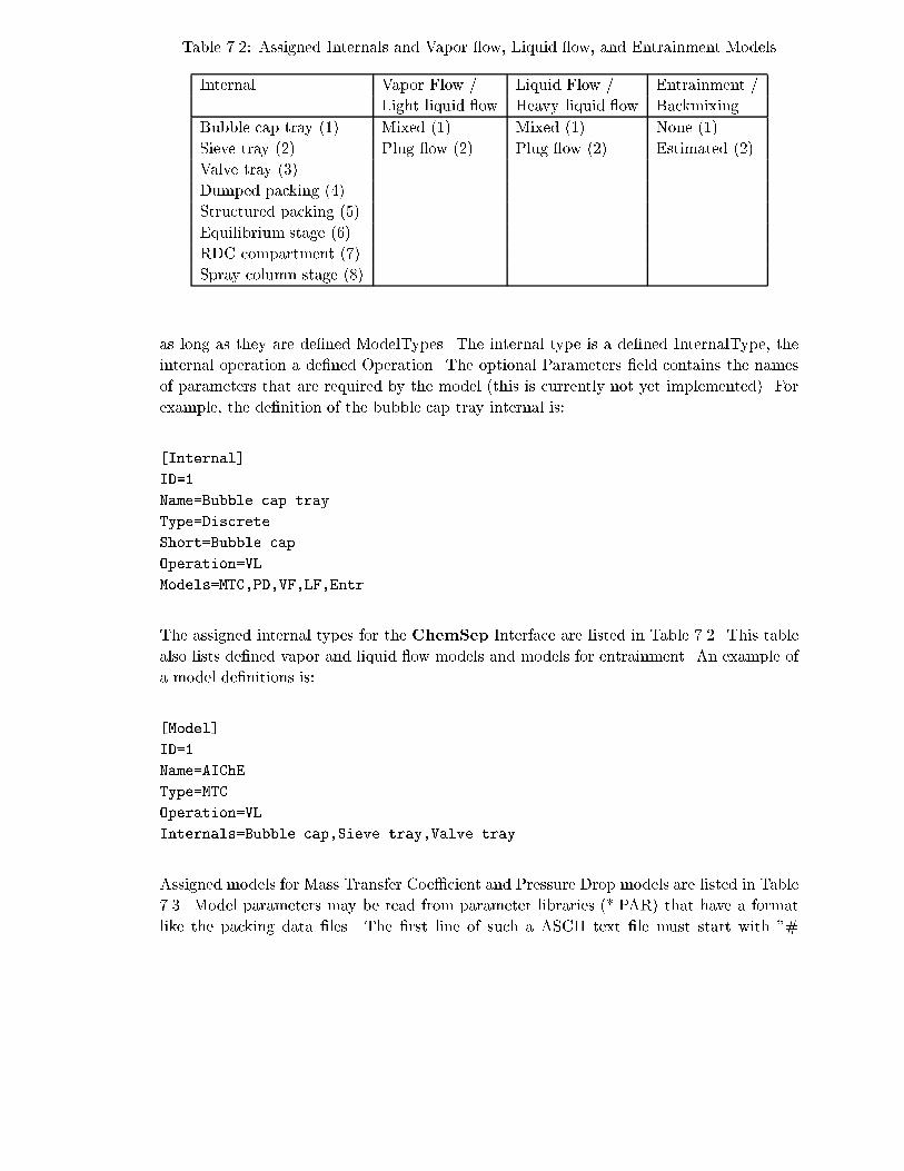
p
Table 7.2: Assigned Internals and Vapor ow, Liquid ow, and Entrainment Models
Internal Vapor Flow / Liquid Flow / Entrainment /
Light liquid ow Heavy liquid ow Backmixing
Bubble cap tray (1) Mixed (1) Mixed (1) None (1)
Sieve tray (2) Plug ow (2) Plug ow (2) Estimated (2)
Valve tray (3)
Dumped packing (4)
Structured packing (5)
Equilibrium stage (6)
RDC compartment (7)
Spray column stage (8)
as long as they are de�ned ModelTypes. The internal type is a de�ned InternalType, the
internal operation a de�ned Operation. The optional Parameters �eld contains the names
of parameters that are required by the model (this is currently not yet implemented). For
example, the de�nition of the bubble cap tray internal is:
[Internal]
ID=1
Name=Bubble cap tray
Type=Discrete
Short=Bubble cap
Operation=VL
Models=MTC,PD,VF,LF,Entr
The assigned internal types for the ChemSep Interface are listed in Table 7.2. This table
also lists de�ned vapor and liquid ow models and models for entrainment. An example of
a model de�nitions is:
[Model]
ID=1
Name=AIChE
Type=MTC
Operation=VL
Internals=Bubble cap,Sieve tray,Valve tray
Assigned models for Mass Transfer Coe�cient and Pressure Drop models are listed in Table
7.3. Model parameters may be read from parameter libraries (*.PAR) that have a format
like the packing data �les. The �rst line of such a ASCII text �le must start with "#

p g
Table 7.3: Assigned MTC and PD Models
Mass Transfer Coe�cient Pressure Drop
AIChE (1) Fixed (1)
Chan Fair (2) Estimated (2)
Zuiderweg (3) Ludwig 1979 (3)
Hughmark (4) Leva GPDC (4)
Harris (5) Billet-Schultes 1992 (5)
Onda et al. 1968 (6) Bravo-Rocha-Fair 1986 (6)
Bravo-Fair 1982 (7) Stichlmair-Bravo-Fair 1989 (7)
Bravo-Rocha-Fair 1985 (8) Bravo-Rocha-Fair 1992 (8)
Bubble-Jet (9)
Bravo-Rocha-Fair 1992 (10)
Billet-Schultes 1992 (11)
Nawrocki et al. 1991 (12)
Chen-Chuang (13)
Handlos-Baron-Treybal (14)
Seibert-Fair (15)
Kronig-Brink-Rowe (16)
Rose-Kintner-Garner-Tayeban (17)
Sherwood (20)
CHEMSEP xxxx" where xxxx must be replaced by the full name of the model (as de�ned
in CHEMSEP.DEF). Upon choosing the library option in the interface the library will be
automatically pre-selected if the name of the library �le is the same as the short name of
its model.
7.9 Author and program information
The authors can be reached through
Regular mail: Ross Taylor / Harry Kooijman
Department of Chemical Engineering
Clarkson University
Potsdam, NY 13699, USA
Telephone: Ross Taylor (315) 268 6652
Harry Kooijman (908) 771 6544
p
Electronic mail: [email protected]
WWW page: http://ourworld.compuserve.com/homepages/HAKooijman
http://www.clarkson.edu/~chengweb/faculty/
taylor/chemsep/chemsep.html
We typed most of the code with the Multi-Edit text editor. It allows us to switch between
the source code of the drivers, interfaces, and column simulation executables, as well as the
text �les for the help and documentation. Each di�erent type of �le has its own commands
associated with it (compile source code, run latex on the documentation, etc.). As the
project is over several hundred thousands lines of source and text, the editor has proven to
be very valuable to us.
The drivers and interfaces are written in Turbo Pascal (version 7.0), the column and ash
programs are written in standard Fortran 77, which we compile with WATCOM Fortran and
link with the CauseWay DOS extender. The source code for the simulation executables has
also been successfully compiled and executed on a range of operating systems and platforms
.
Acknowledgements
WordPerfect is a product of the WordPerfect Corporation. Microsoft Word is a product
of Microsoft Incorporated. DOS4GW is a product of Rational. CauseWay is a product of
Devore software Incorporated. Multi-Edit is a product of American Cybernetics. WAT-
COM F77 is a product of WATCOM Incorporated. Turbo Pascal is a product of Borland
International Incorporated.
References
J.M. Prausnitz, T.F. Anderson, E.A. Grens, C.A. Eckert, R. Hsieh, J.P. O'Connell, Com-
puter Calculations for Multicomponent Vapor-Liquid and Liquid-Liquid Equilibria, Prentice-
Hall, Englewood Cli�s, NJ (1980).
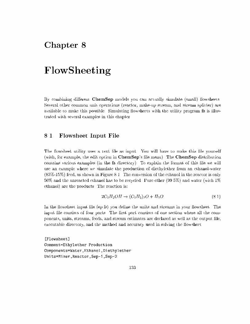
Chapter 8
FlowSheeting
By combining di�erent ChemSep models you can actually simulate (small) owsheets.
Several other common unit operations (reactor, make-up stream, and stream splitter) are
available to make this possible. Simulating owsheets with the utility program fs is illus-
trated with several examples in this chapter.
8.1 Flowsheet Input File
The owsheet utility uses a text �le as input. You will have to make this �le yourself
(with, for example, the edit option in ChemSep's �le menu). The ChemSep distribution
contains various examples (in the fs directory). To explain the format of this �le we will
use an example where we simulate the production of diethylether from an ethanol-water
(85%-15%) feed, as shown in Figure 8.1. The conversion of the ethanol in the reactor is only
50% and the unreacted ethanol has to be recycled. Pure ether (99.5%) and water (with 1%
ethanol) are the products. The reaction is:
2C2H5OH ! (C2H5)2O +H2O (8.1)
In the owsheet input �le (ep.fs) you de�ne the units and streams in your owsheet. The
input �le consists of four parts. The �rst part consists of one section where all the com-
ponents, units, streams, feeds, and stream estimates are declared as well as the output �le,
executable directory, and the method and accuracy used in solving the owsheet.
[Flowsheet]
Comment=Ethylether Production
Components=Water,Ethanol,Diethylether
Units=Mixer,Reactor,Sep-1,Sep-2
133
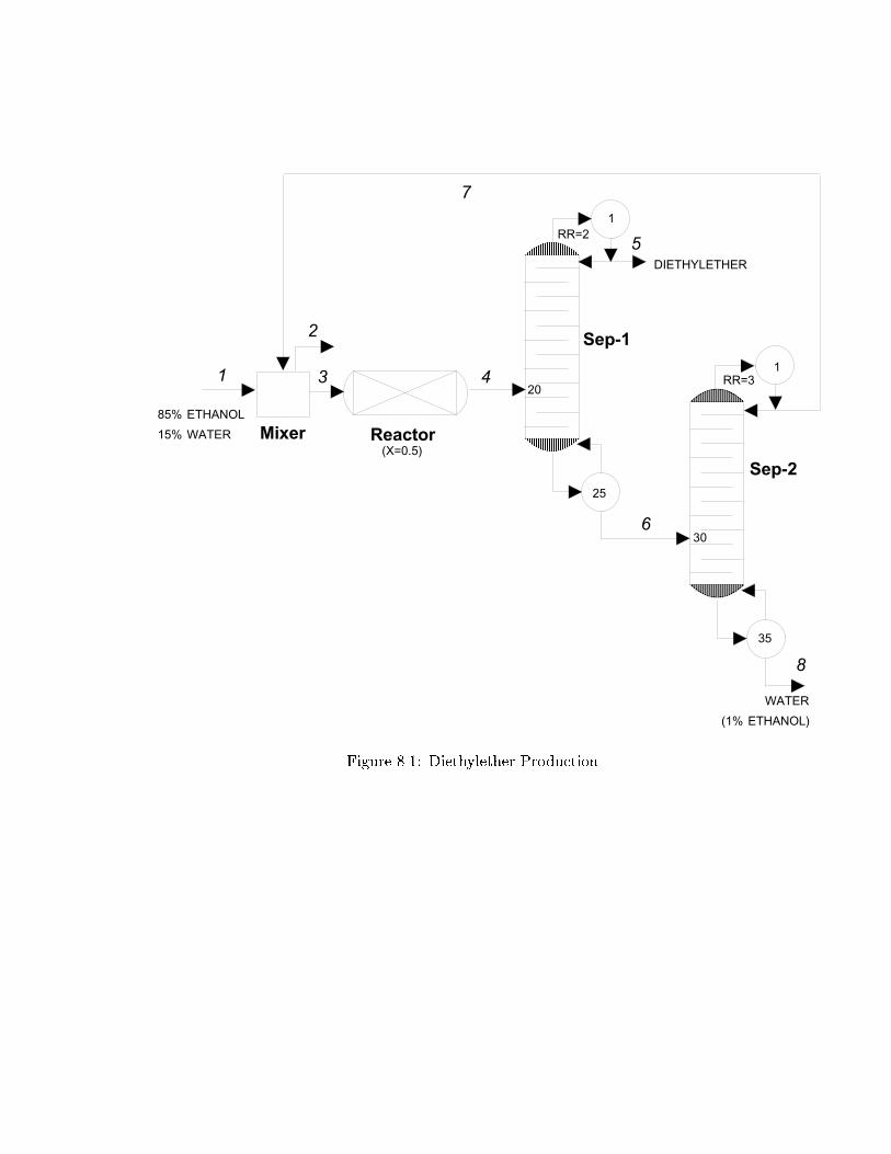
p g
����� �����
��� �
�
�
� �
�
�
�
�
�������
���� ����
�������
���� ���� ��
�����
���� �����
��� �
�
�
��
��
��
��
����
����
Figure 8.1: Diethylether Production

Streams=1,2,3,4,5,6,7,8
Feeds=1
Estimates=7
Output=ep.fs
ExeDir=c:\cs\exes\
MaxIter=20
Method=Direct
Accuracy=0.001
! this is a comment
The section starts with the [Flowsheet] identi�er. The next lines are part of this section
until an empty line is found. You can add (non empty) comment lines in the input �le by,
for example, using any punctuation character to start the line. The owsheet program looks
for the speci�c keywords and if none is found it regards the line as a comment. However,
comment lines do not get copied to the output �le. In each section the keywords can
be di�erent. The keywords are the identi�ers left of the equal signs in the above owsheet
section. They are not case-sensitive and you may enter them in any order (some restrictions
do apply, though).
Comma's are used to separate the various components, streams, units, feeds, or stream
estimates (therefore, they can not be part of a name. This is important as IUPAC com-
ponent names sometimes use comma's. In that case omit the comma's in the component
name. Currently the component names are not checked and it is assumed that the same
components in the same order are used in all the units! This is very important.
The case of the names you specify is not important but the one used in the owsheet section
is used in the rest of the report.
In our example we have the following streams we have given our streams numbers from 1
to 8 (instead of numbers names may also be used). We have only one feed, 1, and we will
make a stream estimate for the recycle (7). Stream 2 is a stream that is not used (we need
it since the ash program that simulates the mixer produces a vapor product stream which
we have to assign). Our unit operations are a mixer, reactor, and two columns (Sep-1 and
Sep-2) where we separate the products. Our output �le is ep.fs (the same name as our
input �le which will be overwritten) and the owsheet method is Direct substitution with a
convergence criterium of 0:001. The maximum number of iterations is speci�ed here as 20.
The next part describes the units and, therefore, can consist of multiple sections. We have
four units in our example. Each unit section starts with the [Unit] identi�er and has �ve
keywords: Name, File, Type, Inlets, and Outlets.
[Unit]
Name=Mixer
File=ep-mix.sep

p g
Type=4g-flash.exe
Inlets=1,7
Outlets=2,3
[Unit]
Name=Reactor
File=ep-reac.sep
Type=reactors.exe
Inlets=3
Outlets=4
[Unit]
Name=Sep-1
File=ep-sep1.sep
Type=4g-neq2.exe
Inlets=4
Outlets=5,6
[Unit]
Name=Sep-2
File=ep-sep2.sep
Type=4g-neq2.exe
Inlets=6
Outlets=7,8
The speci�ed unit name must match the one given in the owsheet section. The unit
�le is the associated data �le, for most units it is the Sep-�le which was generated by
ChemSep. The unit type is the program that must be run to simulate this speci�c unit.
For a ChemSep ash that is 4g- ash.exe, for an equilibrium column 4g-col2.exe, and for
a nonequilibrium column 4g-neq2.exe. This allows you to make your own unit simulation
program that reads a data�le with feed and product section as in a Sep-�le. In the case of
the reactor this is done by the reactors.exe program (which is described below).
The units are connected by in- and outlets streams, which were declared in the owsheet
section above. Be sure to use the same names (case is not important) as otherwise the
owsheet will be incorrect or incomplete. If you just want to analyze a owsheet or not to
simulate the unit it, ommit the unit �le and type (they will not be executed).
[Feed]
Name=1
Temperature=40C
Pressure=1.01325bar
Rate=20mol/s
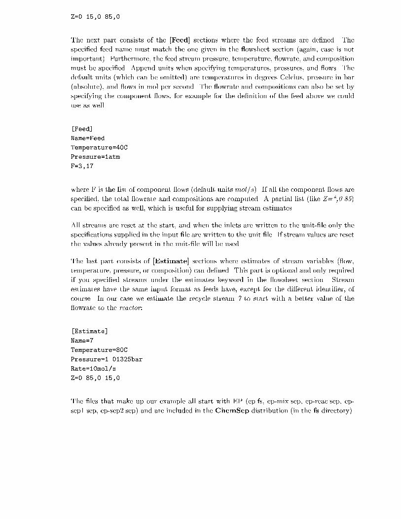
Z=0.15,0.85,0
The next part consists of the [Feed] sections where the feed streams are de�ned. The
speci�ed feed name must match the one given in the owsheet section (again, case is not
important). Furthermore, the feed stream pressure, temperature, owrate, and composition
must be speci�ed. Append units when specifying temperatures, pressures, and ows. The
default units (which can be omitted) are temperatures in degrees Celcius, pressure in bar
(absolute), and ows in mol per second. The owrate and compositions can also be set by
specifying the component ows, for example for the de�nition of the feed above we could
use as well
[Feed]
Name=Feed
Temperature=40C
Pressure=1atm
F=3,17
where F is the list of component ows (default units mol=s). If all the component ows are
speci�ed, the total owrate and compositions are computed. A partial list (like Z=*,0.85)
can be speci�ed as well, which is useful for supplying stream estimates.
All streams are reset at the start, and when the inlets are written to the unit-�le only the
speci�cations supplied in the input �le are written to the unit �le. If stream values are reset
the values already present in the unit-�le will be used.
The last part consists of [Estimate] sections where estimates of stream variables ( ow,
temperature, pressure, or composition) can de�ned. This part is optional and only required
if you speci�ed streams under the estimates keyword in the owsheet section. Stream
estimates have the same input format as feeds have, except for the di�erent identi�er, of
course. In our case we estimate the recycle stream 7 to start with a better value of the
owrate to the reactor:
[Estimate]
Name=7
Temperature=80C
Pressure=1.01325bar
Rate=10mol/s
Z=0.85,0.15,0
The �les that make up our example all start with EP (ep.fs, ep-mix.sep, ep-reac.sep, ep-
sep1.sep, ep-sep2.sep) and are included in the ChemSep distribution (in the fs directory).
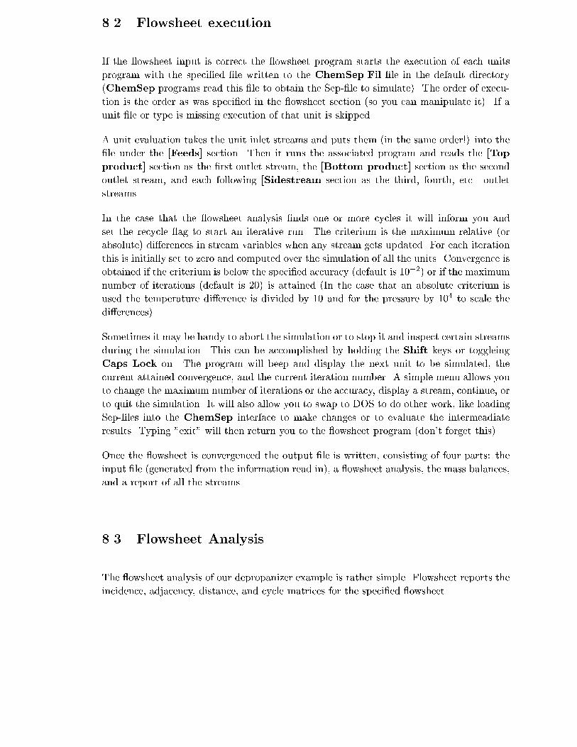
p g
8.2 Flowsheet execution
If the owsheet input is correct the owsheet program starts the execution of each units
program with the speci�ed �le written to the ChemSep.Fil �le in the default directory
(ChemSep programs read this �le to obtain the Sep-�le to simulate). The order of execu-
tion is the order as was speci�ed in the owsheet section (so you can manipulate it). If a
unit �le or type is missing execution of that unit is skipped.
A unit evaluation takes the unit inlet streams and puts them (in the same order!) into the
�le under the [Feeds] section. Then it runs the associated program and reads the [Top
product] section as the �rst outlet stream, the [Bottom product] section as the second
outlet stream, and each following [Sidestream section as the third, fourth, etc. outlet
streams.
In the case that the owsheet analysis �nds one or more cycles it will inform you and
set the recycle ag to start an iterative run. The criterium is the maximum relative (or
absolute) di�erences in stream variables when any stream gets updated. For each iteration
this is initially set to zero and computed over the simulation of all the units. Convergence is
obtained if the criterium is below the speci�ed accuracy (default is 10�2) or if the maximum
number of iterations (default is 20) is attained (In the case that an absolute criterium is
used the temperature di�erence is divided by 10 and for the pressure by 104 to scale the
di�erences).
Sometimes it may be handy to abort the simulation or to stop it and inspect certain streams
during the simulation. This can be accomplished by holding the Shift keys or toggleing
Caps Lock on. The program will beep and display the next unit to be simulated, the
current attained convergence, and the current iteration number. A simple menu allows you
to change the maximum number of iterations or the accuracy, display a stream, continue, or
to quit the simulation. It will also allow you to swap to DOS to do other work, like loading
Sep-�les into the ChemSep interface to make changes or to evaluate the intermeadiate
results. Typing "exit" will then return you to the owsheet program (don't forget this).
Once the owsheet is convergenced the output �le is written, consisting of four parts: the
input �le (generated from the information read in), a owsheet analysis, the mass balances,
and a report of all the streams.
8.3 Flowsheet Analysis
The owsheet analysis of our depropanizer example is rather simple. Flowsheet reports the
incidence, adjacency, distance, and cycle matrices for the speci�ed owsheet.
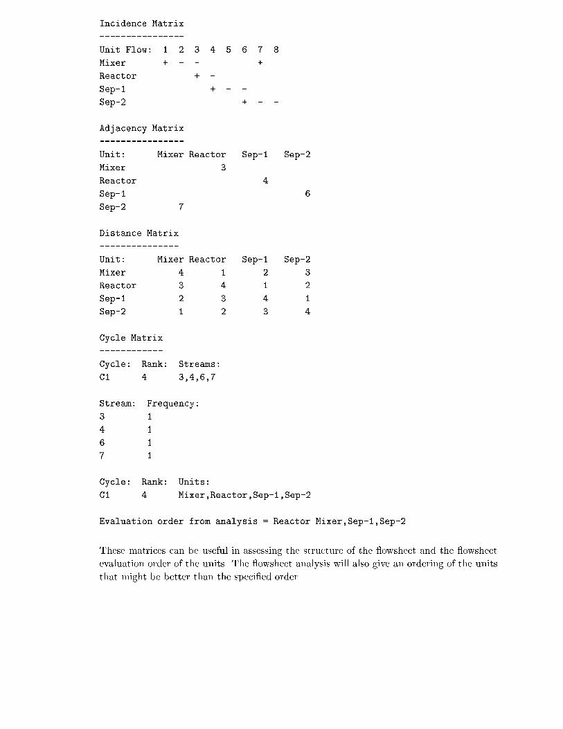
y
Incidence Matrix
----------------
Unit\Flow: 1 2 3 4 5 6 7 8
Mixer + - - +
Reactor + -
Sep-1 + - -
Sep-2 + - -
Adjacency Matrix
----------------
Unit: Mixer Reactor Sep-1 Sep-2
Mixer 3
Reactor 4
Sep-1 6
Sep-2 7
Distance Matrix
---------------
Unit: Mixer Reactor Sep-1 Sep-2
Mixer 4 1 2 3
Reactor 3 4 1 2
Sep-1 2 3 4 1
Sep-2 1 2 3 4
Cycle Matrix
------------
Cycle: Rank: Streams:
C1 4 3,4,6,7
Stream: Frequency:
3 1
4 1
6 1
7 1
Cycle: Rank: Units:
C1 4 Mixer,Reactor,Sep-1,Sep-2
Evaluation order from analysis = Reactor Mixer,Sep-1,Sep-2
These matrices can be useful in assessing the structure of the owsheet and the owsheet
evaluation order of the units. The owsheet analysis will also give an ordering of the units
that might be better than the speci�ed order.
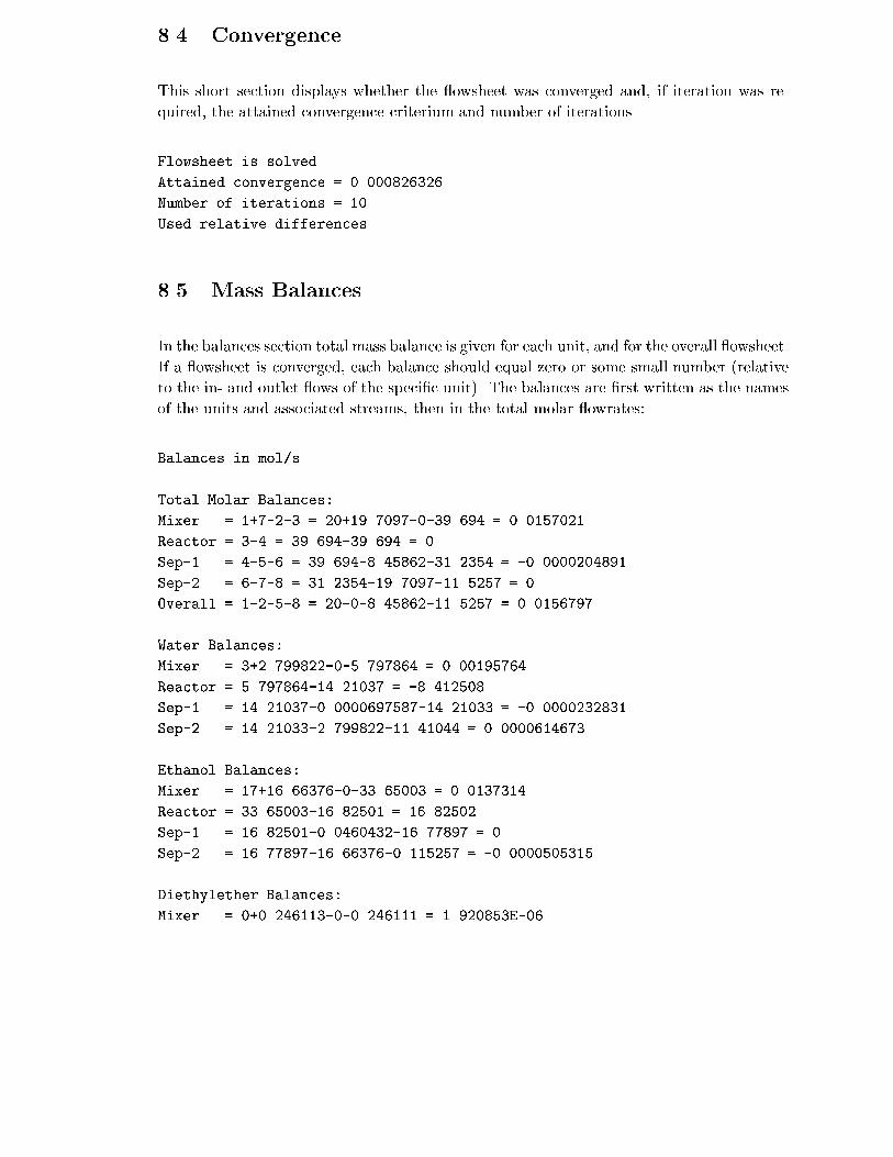
p g
8.4 Convergence
This short section displays whether the owsheet was converged and, if iteration was re-
quired, the attained convergence criterium and number of iterations.
Flowsheet is solved.
Attained convergence = 0.000826326
Number of iterations = 10
Used relative differences.
8.5 Mass Balances
In the balances section total mass balance is given for each unit, and for the overall owsheet.
If a owsheet is converged, each balance should equal zero or some small number (relative
to the in- and outlet ows of the speci�c unit). The balances are �rst written as the names
of the units and associated streams, then in the total molar owrates:
Balances in mol/s
Total Molar Balances:
Mixer = 1+7-2-3 = 20+19.7097-0-39.694 = 0.0157021
Reactor = 3-4 = 39.694-39.694 = 0
Sep-1 = 4-5-6 = 39.694-8.45862-31.2354 = -0.0000204891
Sep-2 = 6-7-8 = 31.2354-19.7097-11.5257 = 0
Overall = 1-2-5-8 = 20-0-8.45862-11.5257 = 0.0156797
Water Balances:
Mixer = 3+2.799822-0-5.797864 = 0.00195764
Reactor = 5.797864-14.21037 = -8.412508
Sep-1 = 14.21037-0.0000697587-14.21033 = -0.0000232831
Sep-2 = 14.21033-2.799822-11.41044 = 0.0000614673
Ethanol Balances:
Mixer = 17+16.66376-0-33.65003 = 0.0137314
Reactor = 33.65003-16.82501 = 16.82502
Sep-1 = 16.82501-0.0460432-16.77897 = 0
Sep-2 = 16.77897-16.66376-0.115257 = -0.0000505315
Diethylether Balances:
Mixer = 0+0.246113-0-0.246111 = 1.920853E-06

p
Reactor = 0.246111-8.658619 = -8.412507
Sep-1 = 8.658619-8.412504-0.246113 = 1.949957E-06
Sep-2 = 0.246113-0.246113-3.203753E-08 = -3.203753E-08
Care must be taken that the individual component balances are also satis�ed, they are
written after the total molar balances. Also, a reactor total molar balance will not be
zero if the reaction changes the number of moles in the mixture. A reactor component
balance will not be zero if that component is involved in one of the reactions that has a
nonzero conversion. In the case of our example we see that the reaction rate is 8.4 mol/s
dietheylether.
8.6 Stream Report
The stream report lists the streams after the execution has stopped.
Stream 1
Temperature (C) 40
Pressure (bar) 1.01325
Flowrate (mol/s) 20
Zwater 0.15
Zethanol 0.85
Zdiethylether 0
Stream 2 is zero
Stream 3
Temperature (C) 58.68402
Pressure (bar) 1.01325
Flowrate (mol/s) 39.694
Zwater 0.146064
Zethanol 0.847736
Zdiethylether 0.00620021
Stream 4
Temperature (C) 49.85001
Pressure (bar) 1.01325
Flowrate (mol/s) 39.694
Zwater 0.357998
Zethanol 0.423868
Zdiethylether 0.218134
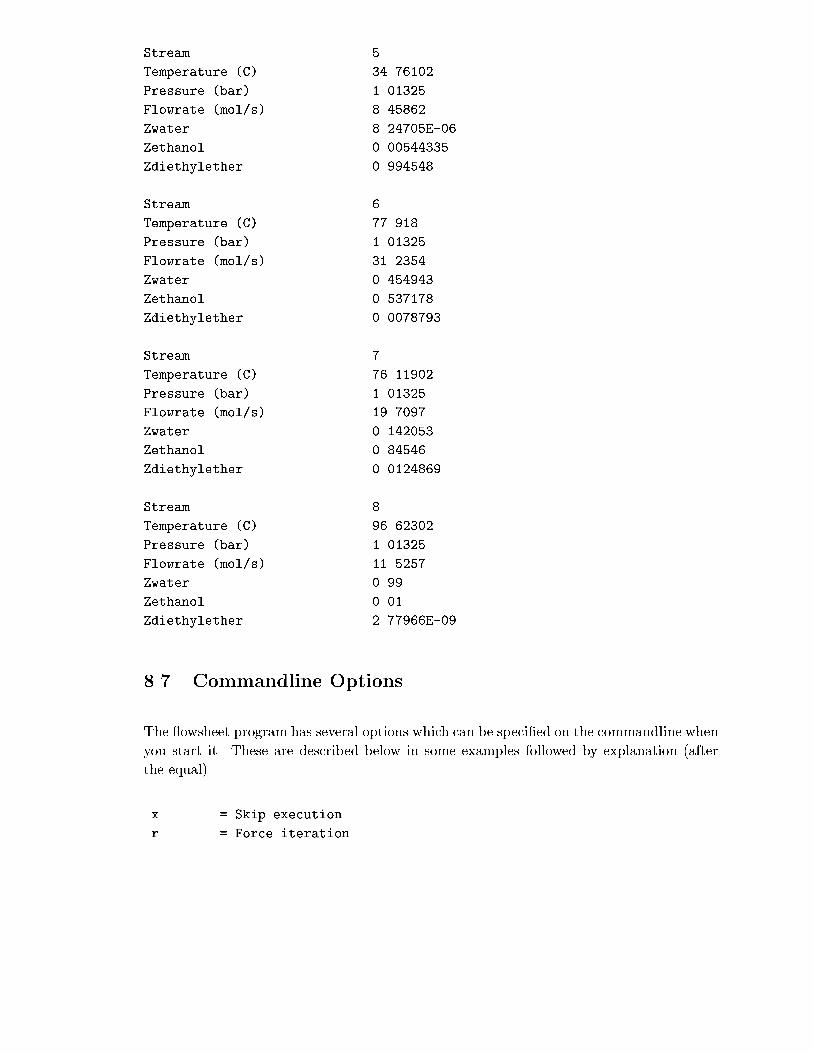
p g
Stream 5
Temperature (C) 34.76102
Pressure (bar) 1.01325
Flowrate (mol/s) 8.45862
Zwater 8.24705E-06
Zethanol 0.00544335
Zdiethylether 0.994548
Stream 6
Temperature (C) 77.918
Pressure (bar) 1.01325
Flowrate (mol/s) 31.2354
Zwater 0.454943
Zethanol 0.537178
Zdiethylether 0.0078793
Stream 7
Temperature (C) 76.11902
Pressure (bar) 1.01325
Flowrate (mol/s) 19.7097
Zwater 0.142053
Zethanol 0.84546
Zdiethylether 0.0124869
Stream 8
Temperature (C) 96.62302
Pressure (bar) 1.01325
Flowrate (mol/s) 11.5257
Zwater 0.99
Zethanol 0.01
Zdiethylether 2.77966E-09
8.7 Commandline Options
The owsheet program has several options which can be speci�ed on the commandline when
you start it. These are described below in some examples followed by explanation (after
the equal).
\x = Skip execution
\r = Force iteration
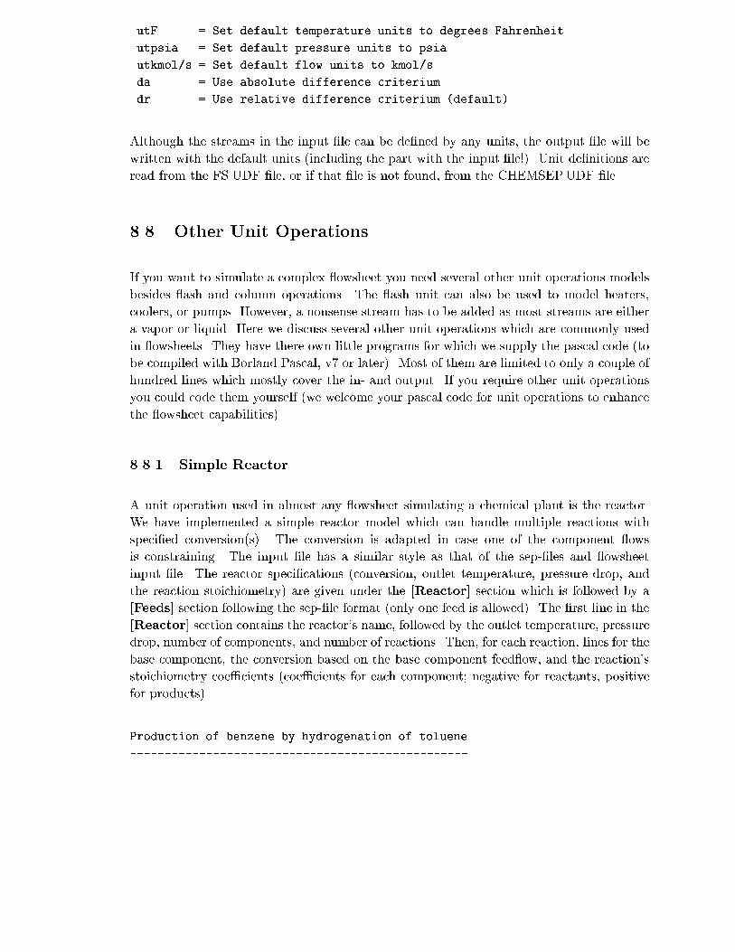
p
\utF = Set default temperature units to degrees Fahrenheit
\utpsia = Set default pressure units to psia
\utkmol/s = Set default flow units to kmol/s
\da = Use absolute difference criterium
\dr = Use relative difference criterium (default)
Although the streams in the input �le can be de�ned by any units, the output �le will be
written with the default units (including the part with the input �le!). Unit de�nitions are
read from the FS.UDF �le, or if that �le is not found, from the CHEMSEP.UDF �le.
8.8 Other Unit Operations
If you want to simulate a complex owsheet you need several other unit operations models
besides ash and column operations. The ash unit can also be used to model heaters,
coolers, or pumps. However, a nonsense stream has to be added as most streams are either
a vapor or liquid. Here we discuss several other unit operations which are commonly used
in owsheets. They have there own little programs for which we supply the pascal code (to
be compiled with Borland Pascal, v7 or later). Most of them are limited to only a couple of
hundred lines which mostly cover the in- and output. If you require other unit operations
you could code them yourself (we welcome your pascal code for unit operations to enhance
the owsheet capabilities).
8.8.1 Simple Reactor
A unit operation used in almost any owsheet simulating a chemical plant is the reactor.
We have implemented a simple reactor model which can handle multiple reactions with
speci�ed conversion(s). The conversion is adapted in case one of the component ows
is constraining. The input �le has a similar style as that of the sep-�les and owsheet
input �le. The reactor speci�cations (conversion, outlet temperature, pressure drop, and
the reaction stoichiometry) are given under the [Reactor] section which is followed by a
[Feeds] section following the sep-�le format (only one feed is allowed). The �rst line in the
[Reactor] section contains the reactor's name, followed by the outlet temperature, pressure
drop, number of components, and number of reactions. Then, for each reaction, lines for the
base component, the conversion based on the base component feed ow, and the reaction's
stoichiometry coe�cients (coe�cients for each component; negative for reactants, positive
for products).
Production of benzene by hydrogenation of toluene
-------------------------------------------------
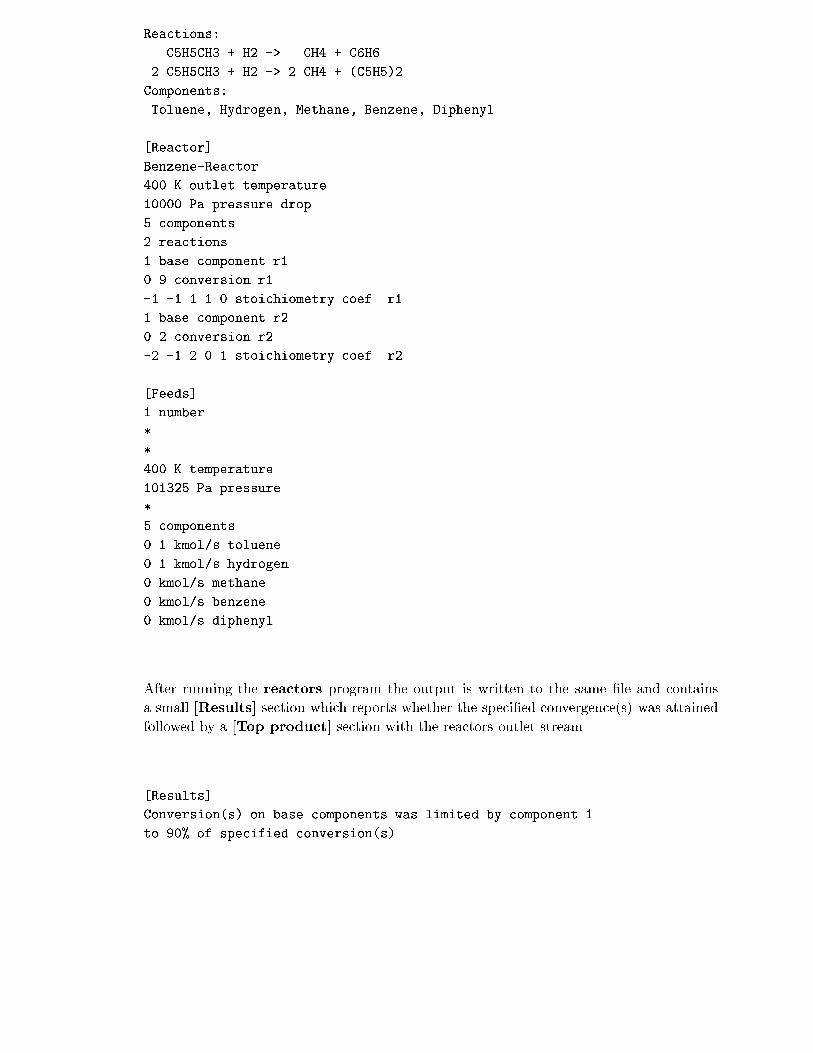
p g
Reactions:
C5H5CH3 + H2 -> CH4 + C6H6
2 C5H5CH3 + H2 -> 2 CH4 + (C5H5)2
Components:
Toluene, Hydrogen, Methane, Benzene, Diphenyl
[Reactor]
Benzene-Reactor
400 K outlet temperature
10000 Pa pressure drop
5 components
2 reactions
1 base component r1
0.9 conversion r1
-1 -1 1 1 0 stoichiometry coef. r1
1 base component r2
0.2 conversion r2
-2 -1 2 0 1 stoichiometry coef. r2
[Feeds]
1 number
*
*
400 K temperature
101325 Pa pressure
*
5 components
0.1 kmol/s toluene
0.1 kmol/s hydrogen
0 kmol/s methane
0 kmol/s benzene
0 kmol/s diphenyl
After running the reactors program the output is written to the same �le and contains
a small [Results] section which reports whether the speci�ed convergence(s) was attained
followed by a [Top product] section with the reactors outlet stream.
[Results]
Conversion(s) on base components was limited by component 1
to 90% of specified conversion(s)

p
If there are multiple reactions and one (or more) of the component feed ows is constraining
the reactions, the conversions are all equally a�ected. For the ether reactor of our example
the reactors input �le looks like:
[Reactor]
Reactor
323 K outlet temperature
0 Pa pressure drop
3 components
1 reactions
2 base component r1
0.5 conversion r1
1 -2 1 stoichiometry coef. r1
[Feeds]
1 Number
1 Feed state T & P
*
331.834 Temperature
101325 Pressure
* Vapour fraction
3 componentflows
0.00579786 Component 1 flow
0.03365 Component 2 flow
0.000246111 Component 3 flow
8.8.2 Make-Up Feeds
Often, when a owsheet contains a recycled solvent or base material, a (small) make-up
feed is required. Since the exact owrate of the make-up feed is unknown, we made a unit
operation that will add a make-up feed (the �rst feed) to another stream (the second feed)
to obtain a speci�ed total owrate.
[Make-up]
Make-up Unit
.06 Total flowrate (always in kmol/s)
[Feeds]
2 Number
1 Feed state T & P
1 stage

p g
373.15 Temperature
100000 Pressure
* Vapour fraction
3 componentflows
0 Component 1 flow
0 Component 2 flow
0.001 Component 3 flow
1 Feed state T & P
1 stage
373.15 Temperature
101325 Pressure
* Vapour fraction
3 componentflows
5.041514E-09 Component 1 flow
0.0000207905 Component 2 flow
0.0598143 Component 3 flow
When the make-up program runs it appends a small [Results] section displays the total
owrate of the make-up feed followed by a [Top product] section containing the resulting
stream.
[Results]
0.0001649 = Make-up flow
Since the make-up feed has to be speci�ed at the beginning this could cause the mass
balances to be incorrect. Therefore, if the owsheet encounters a make-up unit, and the
�rst inlet stream is declared as a feed, its owrate is adapted on writing the output.
8.8.3 Stream Splitter
Similarly to the Make-up unit, owsheets containing recycles sometimes need to purge some
part of the recycle to prevent build-up of various components in the cycle. This means that
the recycle stream must be split into two parts. The splits program implements the stream
split operation. The input �le for the splitter consists of a [Splitter] section, containing
the name of the unit and a splitfactor (which can range from zero to unity):
[Splitter]
Recycle purger
0.1

p
This is followed by the regular [Feeds] section (see for example, the reactor description),
where only one feed may be speci�ed. After running the splits program top and bottom
product streams will be appended to the input �le, where the top product stream has a
owrate equal to the feed owrate multiplied with the splitfactor, and the bottom product
contains the rest of the feed ow.
8.9 Examples
Here we discuss several examples which have been run with the owsheet program. We will
not supply all the details as they can be found in the various �les that are distributed with
ChemSep. Note that all these examples can be solved using the nonequilibrium column
models.
8.9.1 Extractive Distillation (PH)
We need to separate a equimolar mixture of methylcyclohexane (MCH) and toluene, and do
this by extractive distillation with phenol as solvent. The owsheet is shown in Figure 8.2.
Valve trays are used for both the columns using the design mode nonequilibrium simulator.
The Phenol recycle is cooled to 100 C. For a high purity of the products the solvent feed
to MCH/Toluene feed ratio as well as the re ux ratio need to be su�ciently high (for the
extractive column).
8.9.2 Distillation with a Heterogeneous Azeotrope (BW)
Water and butanol form an azeotrope, so that they cannot be seaparated by conventional
distillation. However, at not too high temperature, they form two liquid phases; an aqueous
phase with little butanol and a butanol phase with a large mole fraction of water. We can
use a decanter to separate the two liquid phases. A feed which is predominatly water but
contaminated with butanol (1 mole%) can be separated into two pure products using such a
decanter. The owsheet is shown in Figure 8.3. The �rst column produces a water bottom
product, and the vapor is fed to a condenser/cooler and then to the decanter. There we
obtain a water- and a butanol-rich stream which get recycled to the columns. In a second
column we can then produce butanol as the butanol-rich recycle contains much more butanol
than the butanol-water azeotrope.

p g
�
� �� ��
� �����
� �����
����
������� ������� �
�
�
��
��
��
�
��
���������
���� �� ����
�������
�����
����
����
�
Figure 8.2: Extractive Distillation

p
�� �
� !"# � !"� �"# �"�
�������"# �������"�
����
#$��% ���$� �
���� ����� ����� �����
������ ������
���� � ���� �
���� ����
� �
�
�� ��
��������
�� !�����
Figure 8.3: Distillation with Decanter
p g
8.9.3 Distillation of a Pressure Sensitive Azeotrope (MA)
Methanol and acetone form also an azeotrope. However, the composition of the azeotrope
is sensitive to the pressure. We can make use of this to separate the two components into
pure products by operating two columns at di�erent pressures to change the azeotrope com-
position. The separation of an equimolar feed of methanol and acetone is shown in Figure
8.4. This type of azeotropic distillation is rare as the azeotrope composition needs to be
quite sensitive to the pressure in order to obtain a recycle stream which is not unreasonably
large, and that the pressures are such that no special columns or equipment is required.
8.9.4 Petyluk Columns (PETYLUK)
To lower the energy consumption of separation trains, two columns separating 3 components
can be replaced by one column with a condenser and reboiler plus one column without
condenser and reboiler. The feed is fed to this (�rst) column, which receives a vapor to the
bottom and a liquid at the top from the (second) column with the condenser and reboiler.
In turn, the products of the �rst column are fed into the second column at the sidestream
stages. Figure 8.5 shows such a con�guration for the separations of three alcohols. To
get this owsheet to run requires that you can solve both the columns separately, which is
not easy. The second column needed some speci�c user initialization information to run.
Afterwards convergence can be obtained more easily by using the old results as initialization.
8.9.5 Extraction with Solvent Recovery (BP)
Extraction can be used to separate aromatics from parra�ns. This is a common type of
separation in the crude oil re�ning. a simpli�ed example is shown here where we separate
benzene from n-pentane, using an extraction with sulfolane as solvent. The extractor is
a rotating disk contactor (RDC) operating at 50 C. The solvent is recovered from the
extract by "ordinary" distillation. UNIQUAC parameters for the components are given
in Table 8.1. The extraction is dependent on the temperature as can be seen from the
interaction parameters, which can be used to manipulate the separation. See Figure 8.6 for
the owsheet.

p
����
&'� "�
����"�
&��� ��
���$� �
&'� "�
����� �����
�� ��� �����
!���
�
�
��
��
��
��
��
�� ���
�� ���
�
Figure 8.4: Azeotropic Distillation at Two Pressures

p g
����
�"�% !$� �
("���$� �
�"���$� �
)�
*�
*�
)�
����� �
����� �
���"#��#����
�� �" !�����
���" !�����
��
�
�
��
��
��
Figure 8.5: Petyluk Columns
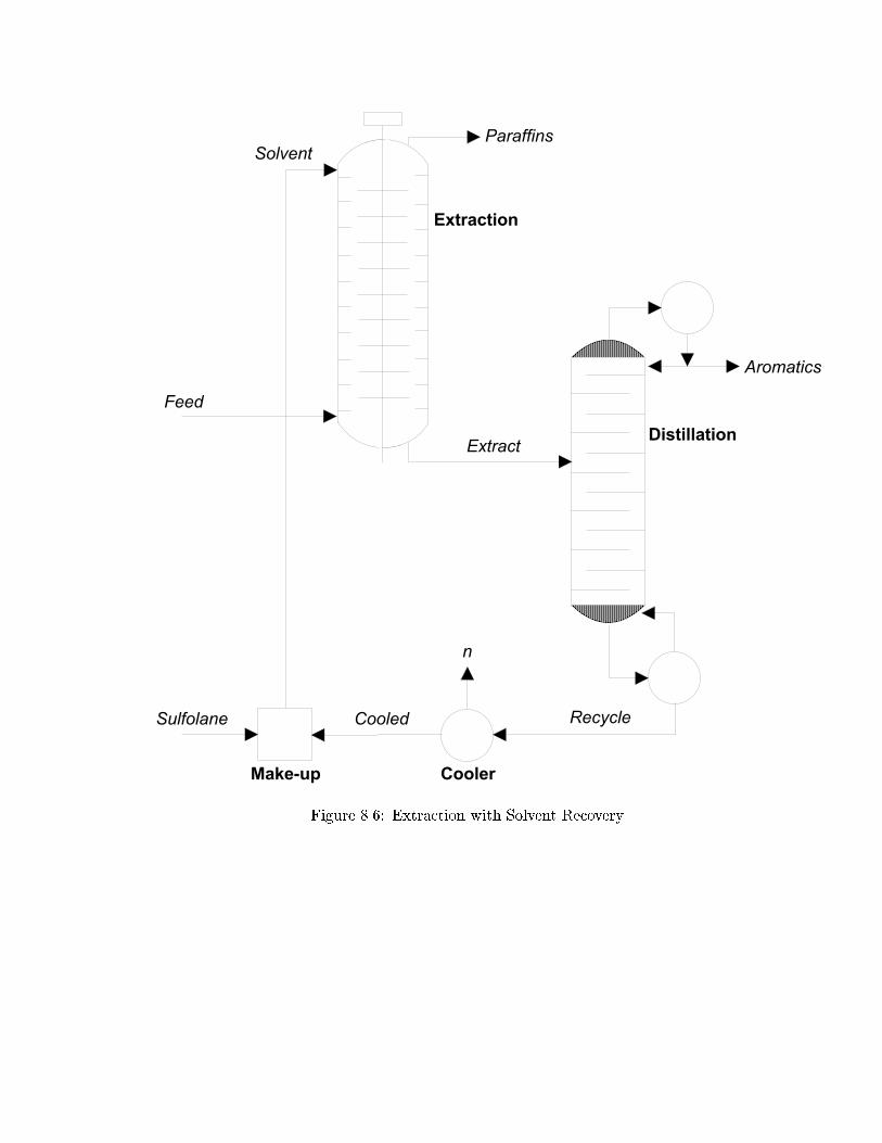
p
���� �� ����
"������
���������
����
���+ �$��
�$%$++(��
&% �$�(��
�������
�
���
,-�%$��
� �����
Figure 8.6: Extraction with Solvent Recovery

p g
Table 8.1: UNIQUAC LLE interaction parameters (K)
Components i-j Aij Aji
25oC:
pentane-benzene 295.38 -171.63
pentane-sulfolane 532.04 187.84
benzene-sulfolane 151.02 -36.08
50oC:
pentane-benzene 179.86 -95.70
pentane-sulfolane 375.93 247.77
benzene-sulfolane 131.51 -6.28

Chapter 9
ChemProp
In this chapter we will brie y discuss ChemProp which allows us to obtain physical prop-
erty predictions in an interactive manner.
9.1 Input
ChemProp requires you to select the components in the mixture just like ChemSep. Un-
der conditions the pressure, temperature, and overall compositions need to be speci�ed,
similarly to the feed speci�cations for a distillation column in ChemSep. The phase equi-
librium determines the type of equilibrium calculation. If set to none, no phase equilibrium
calculations are done. If set to VLE then vapor and liquid equilibrium is calculated. The
vapor and liquid properties are calculated given the compositions from the phase calcu-
lations. If a phase is absent, no physical properties are calculated. Under properties the
selection of the thermodynamic and physical property models needs to be made. If data is
reuired for the selected models this is also entered here. This selection of models is identical
to that in ChemSep.
9.2 Results
9.2.1 Component properties
The component properties table displays the pure component data for all the components.
The properties that are temperature dependent are evaluated at the speci�ed temperature
under the conditions. You can press F8 to change the conditions, and F9 to change the
155
p p
models.
9.2.2 Mixture properties
The mixture properties table displays the mixture physical properties, such as densities,
viscosities, heat capacity, thermal conductivity, and surface tension. If speci�ed, a ash
calculation is calculated to determine the phase compositions. Then the properties are
calculated for each of the existing phases at the phase compositions. If no phase equilibrium
is calculated the mixture physical properties are calculated for both phases at the overall
compositions as speci�ed in the conditions. You can press F8 to change the conditions, and
F9 to change the models.
9.2.3 Tables
The table option displays a speci�c property, or a set of properties, as function of a tem-
perature, pressure, or composition range. The number of points can be set as well as the
range limits. You can press F8 to change the conditions, and F9 to change the models.
9.2.4 Graphs
The graph option displays the same information as in the table option but in graphical
form. If multiple properties were speci�ed the user must select which axis is to be used for
displaying each property. You can press F8 to change the conditions, and F9 to change the
models.
9.2.5 Phase diagrams
Binary and ternary phase diagrams are supported. Constant temperature (Pxy) or pressure
(Txy) binary diagrams can be drawn, or XY diagrams at constant pressure or temperature.
A three dimensional TPxy diagram can also be drawn where the user can specify sets of
temperatures and pressures where XY diagrams are to be calculated and drawn.
For the ternary diagrams only the diagrams at constant pressure (Txy) and pressure (Pxy)
are available. For these diagrams the residu curve maps can be calculated. In these ternary
diagrams, residu curves can be drawn on the bubble temperature surfaces, as well as their
projections on the bottom of the ternary diagram. The number of residu curves can be
speci�ed.

9.2.6 Di�usivities
Liquid and vapor Maxwell-Stefan as well as Fick di�usivities can be drawn. Also the inverse
B matrix and Gamma matrix can be drawn for a ternary mixture. Temperature and pressure
can be speci�ed, or the temperature can be calculated from the phase equilibrium. The
number of lines in the �gure determines the detail in the surfaces that is visible.
9.3 Various
Miscellaneous ChemProp �les include:
� CHEMPROP.UDF: Units De�nition File
� CHEMPROP.HLP: HeLP �le
� CHEMPROP.CNF: the default CoNFiguration �le
� CHEMPROP.SCR: the additional introduction SCReen(s)

p p

Chapter 10
ChemLib
This chapter discusses the pure component data librarian and the format of the binary and
text Pure Component Data �les. ChemSep and ChemProp need these component data
to calculate the required thermodynamic and physical properties. Therefore, they are an
essential part in the package. Extending the supplied libraries (or making your own) is
necessary when you want to use components that are not part of the standard library.
10.1 Pure Component Data �les
Two types of PCD �les can be used: binary and text. The binary �les were initially used to
facilitate fast lookup and searching of component data. With todays bigger hard disks and
faster machines, the reasons for using binary �les have deminished. However, the standard
libraries are in binary read-only format as it makes it more di�cult to make changes to
the library. This reduces the chance a user's problem is caused by bad modi�cations of the
standard PCD library.
However, the ChemSep interface and calculation programs can also handle component
data �les in text format. The USERPCD program used to generate this type of �les to
allow users to add their own components to ChemSep. With the inclusion of ChemLib
this has become easier and USERPCD is no longer supplied. ChemLib can edit binary
PCD �les and export/import to and from text format component data �les.
For a proper functioning of the models in ChemSep it is pertinent that the correct com-
ponent data is used. Inspection of the component data used in any simulation is highly
recommended. That is why their is a special link to the ChemLib program in the Chem-
Sep interface (at the bottom of the input menu). This section we will describe the types
of data in the PCD �les and their typical usages.
159

p
10.1.1 Name and library index
We have adopted the same component names as used by DIPPR (as DIPPR is becoming
an industry standard). The components ID numbers (Library Index) are based on the
system developed at Penn State University (also adopted by DIPPR). Some common used
components ID numbers are:
Methane 1 Water 1921
Ethane 2 Chloroform 1521
Propane 3 Methanol 1101
i-Butane 4 Ethanol 1102
n-Butane 5 Acetone 1051
cycloPentane 104 2-Butanone (MEK) 1052
i-Pentane 8 Benzene 501
n-Pentane 7 Toluene 502
cycloHexane 137 m-Xylene 506
n-Hexane 11 p-Xylene 507
n-Heptane 17 Phenol 1181
n-Octane 27 MethylCycloHexane 138
n-Nonane 46 Nitrogen 905
n-Decane 56 Carbon dioxide 909
10.1.2 Structure
The structure is a string representation of the components chemical structure (as far is
possible) which enables ChemSep to search components by chemical structure parts. It
also stores the atoms that make up the molecule. This can be used to generate the overall
formula (which is also displayed) or to in estimation methods that use atom contributions.
10.1.3 Family
This indicates the family to which the molecule belongs (alkanes, alkenes, acids, etc.). The
family type can be used in the model selection for di�usivities and other properties.
10.1.4 Critical properties and triple/melting/boiling points
The critical properties consist of the critical temperature (K), pressure (Pa), volume (m3),
and the critical compressibility factor. These properties are used in many models, most im-
portantly thermodynamic models such as equations of state or corresponding states models.

The normal boiling point (K), melting point (K), and triple point (K, Pa) are used in
temperature checks during the simulation. ChemSep does not (yet) perform any stability
calculations with solids and therefore has only simple warnings regarding this matter. The
normal boiling point is used in various thermodynamic models (for example for the vapor
pressure).
10.1.5 Molecular parameters
These consist of properties such as the molecular weight (kg=kmol) and liquid molar volume
(m3=kmol, at the normal boiling point). The molecular weight is required for all the mass
calculations as well as many other things such as concentrations. The acentric facto (also
know as =omega) is most noticably used in the equation of states and corresponding states
methods. Solubility parameter is used in the Regular activity coe�cient model. The Van
der Waals volume (m3=kmol) and area (m2=kmol) are used for estimating UNIQUAC R
and Q properties (used to calculate surface and volume fractions).
10.1.6 Heats/energies/entropies
Here we de�ne the IG heat and Gibbs energy of formation (J=kmol) that can be used in
the calculation of chemical equilibria. Entropy calculations require the IG absolute entropy
(J=kmol). The heats of fusion melting point and of vaporization normal boiling point
(J=kmol) can be used in thermodynamic models and calculating enthalpies (the di�erence
in enthalpy between vapor and liquid is given by the enthalpy of vaporization for example).
The standard net heat of combustion (J=kmol) can be used for ?
10.1.7 Temperature correlations
Various properties are very dependent on the absolute temperature. The DIPPR library
has an extensive set of these properties that we also included in the component data: solid
density (kmol=m3), liquid density (kmol=m3), vapour pressure (Pa), heat of vaporisation
(J=kmol), solid heat capacity (J=kmol=K), liquid heat capacity (J=kmol=K), ideal gas
heat capacity (J=kmol=K), second virial coe�cient (m3=kmol), liquid viscosity (Pa:s),
vapour viscosity (Pa:s), liquid thermal conductivity (W=m=K), vapour thermal conductiv-
ity (W=m=K), and surface tension (N=m). We added several methods that are from the
book "Properties of Gases and Liquids" by Reid, Prausnitz and Sherwood (3rd Ed.) and
Reid, Prausnitz and Poling (4th Ed.): the ideal gas heat capacity (J=kmol=K), heat of
formation (J=kmol), Antoine vapor pressure (Pa), and the liquid viscosity (Pa:s).

p
The type of temperature correlation is determined by an equation number (see the descrip-
tion of the property models). The minimum and maximum temperature (K) describe the
working range of the correlation. Five parameters (A through E) are available. Their units
will depend on the correlation type.
The most important temperature correlations are the ideal gas heat capacities. Either one
of the two heat capacity correlations must be known in order to calculate any enthalpies in
ChemSep.
10.1.8 Miscellaneous parameters
The V star property is used in liquid volume calculations. The Lennard Jones diameter and
energy can be used in vapor viscosity and di�usivity calculations. The Rackett parameter is
used in the estimation of liquid volumes. It can be used to calculate the volume correction
for the SRK EOS for example. The Fuller-Schettler SigmaV is used in the Fuller et al.
method for estimating vapor di�usivities. The surface tension at the normal boiling point
as well as the Parachor can be used in surface tension calculations. The speci�c gravity is
used in the regular model and is estimating properties for petroleum pseudo components.
The Chung association parameter is used for liquid di�usivity estimation.
10.1.9 Thermodynamic model parameters
There are properties that function as parameters for thermodynamic models. To make these
real model parameters for the models in question, they are de�ned separately. These are
the acentric factor for the SRK cubic equation of state and the Chao-Seader method, the
molar volume for the Wilson activity coe�cient model and the Chao-Seader method, and
the solubility parameter for the Chao-Seader method. Other component thermodynamic
parameters are the R,Q, and Q' constants for the UNIQUAC activity coe�cient model and
the k1, k2, and k3 parameters for the PRSV equation of state.
10.1.10 Group contribution methods
ChemSep supports the UNIFAC and ASOG group contribution methods for calculating
activity coe�cients in vapor-liquid equilibria. The UNIFAC is also available for liquid-
liquid equilibria calculations. Three other group contribution methods are to be included in
the ChemSep program: GC EOS (for VLE), IDIFAC (for di�usivities), and the modi�ed
UNIFAC. These are currently not used.

10.2 Making a new library
To start a new library select the new option from the �le menu, and enter the name of
the new library and a description for the library when prompted for an "info string". The
library will contain no components, and you will have to use the Edit menu to add new or
import components.
10.3 Editing a library
The edit menu allows you to change the library label, edit component data, delete / move /
import / export / update components, check component data presence, estimate component
data, and de�ne Pseudo components (from a �le with normal boiling points and speci�c
gravities).
10.3.1 Edit/View Library Label
The label serves as a description of the library.
10.3.2 Change/Browse Component
This option will let you select a component of which you want to edit or peruse the property
data. After entry ChemLib will prompt you whether you want to write the information
to the library. Be careful! Acknowledging to write the information immeadiately updates
the library and there is no way to recover the previous data if you made a mistake.
10.3.3 Deleting Components
To delete components from a library, select the component you want to delete. You can
only delete one component at a time.
10.3.4 Moving Components
To move components from the current library to somewhere else, use the Move option in
the Edit menu. Select the component to move and a library where to move the component
to. You can only select one component to move at a time.

p
10.3.5 Importing/New Components
You can import or add a new component into the loaded library, either by entering a new
component from the keyboard or by importing it from a text �le with the component data,
from another library, or from a DIPPR data �le. The latter are text �les with component
data which follow the DIPPR format. It is also possible to only import one type of property
for multiple components from a text �le.
10.3.6 Exporting Components
Simarly to importing you can export component data of components residing in the loaded
library to the screen, to a text �le, or to another library. It is also possible to export one
property for a selection of components to a text �le.
10.3.7 Updating Components
Instead of importing you can update the component data. This means that only unde-
�ned (empty) data �elds will get imported. Component data from multiple sources can be
gathered this way.
10.3.8 Checking Components
Once you have collected component data you might want to check it for missing data. Use
the check option to write a report to a text �le of a selection of components in the current
library. Di�erent levels of checking are allowed: essential data, preferred data, optional
data, reactions data, or all data.
10.3.9 Estimating Components
If you want to estimate essential data that is missing you can do so with various estimation
methods for a selection of components. First select the estimation methods, than the
components for which to estimate the data. You �nd a description of the estimation below,
under estimating properties for a new component.

10.3.10 Making Pseudo Components
Pseudo components can be generated when you have a list of the normal boiling temperature
(1 atm) and speci�c gravity of the mixture for which you want to make a pseudo compo-
nent de�nition. The method assumes you are trying to estimate properties of a petroleum
derivative.
10.3.11 Estimating Properties for a New Component
When you import a new component from the keyboard, the component will be completely
unde�ned. Select the last option, estimate properties, to estimate component property
data. The Joback (1984) and Constantinou & Gani (1994) methods are using the UNIFAC
groups to estimate the properties. The Riazi Daubert (1980), Twu (1986), and Soave (1998)
methods use the normal boiling point temperature and the speci�c gravity to estimate
component properties. Only data that is not yet de�ned will be calculated, and the data
that is already present can be used in the estimation of other properties.
10.3.12 UNIFAC methods
The Constantinou & Gani (GC) group method uses the UNIFAC groups and can be used
directly. However, the groups in the Joback method di�er from the UNIFAC groups and
a translation table was set up from UNIFAC to Joback groups (this table is not complete
and could potentially create errors). The properties that are estimated are the critical
temperature, pressure, and volume (hence, also the compressibility), the normal boiling
point, and the melting point. The (RPP) gas heat capacity, heat of formation, and the
gibbs energy of formation can also be estimated using either the Joback group method, or
a group method described in Perry's (6th Ed.!) or by Harrison and Seaton (1988) which
only predicts the heat capacity.
The Chickos method is used to approxiomate the heat of fusion at the melting tempera-
ture. This is a group method that requires some knowledge of the rings and the number
of functional groups that cannot be easily extracted from the UNIFAC groups. Therefore,
the method has been partially implemented. As the method directly multiplies the melting
temperature with the entropy of fusion, a large error can be expected if the melting tem-
perature is estimated. Thus, errors for the estimated heat of fusion can easily be large. An
average error of 25% was calculated for four test molecules.
If we are using the Joback method the acentric factor is calculated using the Lee-Kesler
equation, otherwise it is estimated with the GC method. The UNIQUAC R and Q parame-

p
ters are determined by the UNIFAC groups, and the van der Waals properties are computed
directly from R and Q. The molecular weight is calculated by parsing the atoms in the UNI-
FAC groups (for some groups this willNOT work) and so is the Fuller et al di�usion sigma
volume and the components formula (which is used as the name). The heat of vaporization
at Tb is computed from Vetere's correlation. The Rackett parameter is computed with:
ZRa = 0:29056 � 0:08775! (10.1)
and the Parachor with the method by Zuo et al.. The heat of combustion is estimated with
the method of Cardozo and the heat of formation. The absolute entropy is correlated by a
method by Kooijman (1998):
S(298) =Xi
Si +�Sf (298) (10.2)
where the entropy of formation is computed from the Heat and Gibbs free energy of forma-
tion:
�Sf (298) = �Hf (298) ��f (298)=over298 (10.3)
and the Si is the absolute entropy of the element i. To compute this sum the following
expression is used when the number of atoms in the molecule are known:
Si = 105 (0:0574Nc + 1:30571Nh=2 + 2:02682Nf =2 + 2:22972Ncl=2 + 1:5221Nbr=2 + 1:1614Ni=2 + 0:32054N
(10.4)
Here Nc is the number of carbon atoms, Nh the number of hydrogen atoms, etc. (the state
of the elements is gas, except for C, S, and I2 which are crystals, and Br2 which is a liquid
at 298 K and 1 atm. Source Perry's 7th Ed.).
10.3.13 Tb and SG methods
The methods that use the normal boiling point temperature and the speci�c gravity meth-
ods are typically applied for estimating properties of petroleum distillate cuts. The Riazi
Daubert (1980) is the most comprehensive. It estimates the molecular weight, critical
pressure and volume, liquid volume, refractive index, latent heat, and speci�c heat. From
these the acentric factors is calculated with the Lee Kesler method. From correlations from

Speight (1991) and Soave (1998) the atomic composition is estimated, as well as the heat
of combustion, the Fuller di�usion volume, and the Antoine vapor pressure parameters.
The Twu (1986) method predicts the molecular weight, critical pressure, temperature and
volume. It uses the Lee-Kesler method to estimate the acentric factor. The Soave (1998)
method predicts the critical pressure and temperature. It uses the Lee-Kesler method to
estimate the acentric factor.
10.4 Other ChemLib Files
Miscellaneous ChemLib �les include:
� CHEMLIB.UDF: Units De�nition File
� CHEMLIB.HLP: HeLP �le
� CHEMLIB.CNF: the default CoNFiguration �le
� CHEMLIB.SCR: the additional introduction SCReen(s)
10.5 References
R.L. Cardozo, AIChE J., Vol. 32 (1986) pp. 844.
J.S. Chickos, C.M. Barton, D.G. Hesse, J.F. Liebman, J. Org. Chem., Vol. 56 (1991) pp.
927.
L. Constantinou, R. Gani, \New Group Contribution Method for Estimating Pure Com-
punds", �AIChE J., Vol. 40, No. 10 (1994) pp. 1697-1710.
L. Constantinou, R. Gani, \Estimation of the acentric factor and the liquid molar volume
at 298 K using a new group contribution method", Fluid Phase Equil., Vol. 103 (1995) pp.
11-22.
B.K. Harrison, W.H. Seaton, Chem. Eng. Ind. Res., Vol. 27 (1988) pp. 1536.
K.G. Joback, MS Thesis Chem.Eng., MIT, Cambridge, Mass., June (1984).
p
B.I. Lee, M.G. Kesler, AIChE J., Vol. 21 (1975) pp. 510.
Perry's Chemical Engineers Handbook, McGraw Hill, 6th and 7th Ed. (1997).
M.R. Riazi, T.E. Daubert, \Simplify property predictions", Hydrocarbon Processing, Mar
(1980) pp. 115-116.
J.G. Speight, The Chemistry and Technology of Petroleum, 2nd Ed., Marcel Dekker Inc.,
New York (1991).
G.S. Soave, \Estimation of the critical constants of heavy hydrocarbons for their treatment
by the Soave-Redlich-Kwong equation of state", Fluid Phase Equilibria, Vol. 143 (1998)
pp. 29-39.
C.H. Twu, \An internally consistant correlation for predicting the critical properties and
molecular weights of petroleum and coal-tar liquids", Fluid Phase Equilibria, Vol. 16 (1984)
pp. 137-150.
M.T. Tyn, W.F. Calus, Processing, Vol. 21, No. 4 (1975) pp. 16.
Y-X. Zuo, E.H. Stenby, Parachor, Can. J. Chem. Eng., Vol. 75 (1997) pp. 1130.

Index
This chapter will contain an index of all subjects, keywords, models etc.
169


