Page 1
CHENGYAN SUN
HYDROSTATIC-MECHANICAL POWER SPLIT CVT
Master of Science Thesis
Examiners: Professor Kalevi Huhtala Msc. Janne Uusi-Heikkilä
Examiner and topic approved at the faculty council meeting of Automation, Mechanical and Materials engineering on 8th of September 2010
Page 2
Abstract
TAMPERE UNIVERSITY OF TECHNOLOGY Master’s Degree Program in Machine Automation CHENGYAN, SUN: Hydrostatic-Mechanical Power Split CVT Master of Science Thesis, 52 pages, 6 Appendix pages January 2011 Major: Mechatronics Examiners: Professor Kalevi Huhtala, Msc. Janne Uusi-Heikkilä Keywords: hydrostatic, mechanical, power split, CVT, Planetary, steady state characteristics, application, transmission efficiency, work cycle suitability, power range suitability The customer requirements of low fuel consumption, low emissions, and high
performance require new technical solutions allowing for optimization of the entire
drive train, CVT technology, continues to emerge as a key technology for improving the
fuel efficiency of vehicle with internal combustion engines, because it allows the engine
to operate at peak efficiency and reduces the operation difficulty. Hydrostatic-
mechanical power split CVT is a special CVT technology, it is suitability for high
power density applications. It lies in between the pure hydrostatic and the pure
mechanical transmissions.
This thesis involved the study of the hydrostatic-mechanical power split CVT
technology. Based on the theoretical model, the steady state characteristics were studied
to display the advantage and disadvantage of this transmission, then a market
application review was made to show the practical application of this technology,
finally suitability study was carried out based on dynamic model, to find out the
working cycle suitability and power range suitability of this transmission technology.
Page 3
Preface
I would like to thank Professor Kalevi Huhtala for the interesting topic he provided, and
his useful suggestions. I would like to extend my gratitude to Msc. Janne Uusi-Heikkilä
for his wise counsel and constructive comments. A special thanks to Dr. Mikko Erkkilä
for providing me useful materials and warm help.
In addition, I would like to thank my parents, for their love, effort and guidance to
make me a thoughtful man. Finally, I would like to thank my love Qiu Dan, for her
love, which makes my life wonderful and promising.
Chengyan Sun
Tampere, 2011
Page 4
Table of Contents
Nomenclature ................................................................................................................................ i
1 Introduction ...........................................................................................................................1
1.1 Background ..................................................................................................................1
1.2 Object ............................................................................................................................2
1.3 Structure of the thesis .................................................................................................2
2 Fundamental theory ............................................................................................................3
2.1 The principle of hydrostatic-mechanical power split CVT .....................................3
2.2 Classification of the hydrostatic mechanical power split CVT ..............................4
2.3 The components of the hydrostatic mechanical power split CVT ........................5
3 Steady state modeling of basic power split circuit..........................................................6
3.1 Input coupled circuit ....................................................................................................6
3.1.1 Power flow ............................................................................................................6
3.1.2 Power distribution diagram ................................................................................7
3.1.3 Input coupled model ............................................................................................8
3.2 Output coupled ......................................................................................................... 11
3.2.1 Power flow ......................................................................................................... 11
3.2.2 Power distribution diagram ............................................................................. 13
3.2.3 Output coupled model...................................................................................... 14
3.3 The variable bridge transmission ........................................................................... 16
3.4 Steady state hydrostatic transmission models .................................................... 16
3.4.1 Pump model ...................................................................................................... 16
3.4.2 Motor model ...................................................................................................... 17
3.5 Summary ................................................................................................................... 18
4 Steady State Characteristics .......................................................................................... 19
4.1 Input coupled speed summation ............................................................................ 19
4.2 Output coupled simulation ...................................................................................... 22
4.3 Summary ................................................................................................................... 25
5 HMPS-CVT Application ................................................................................................... 26
5.1 The Claas-Jarchow HM-8 and HM-II ..................................................................... 26
5.2 The Fendt Vario ........................................................................................................ 27
5.3 The Steyr S-Matic for Steyr, Case, New Holland ................................................ 29
5.4 The ZF Eccom for Deutz-Fahr, John Deere, Claas ............................................ 30
5.5 Yanmar CVT ............................................................................................................. 32
Page 5
5.6 Summary ................................................................................................................... 34
6 Suitability study ................................................................................................................. 35
6.1 Diesel engine ............................................................................................................ 35
6.2 Model of hydrostatic transmission ......................................................................... 36
6.3 Tire road connection ................................................................................................ 38
6.4 Drive wheel model .................................................................................................... 38
6.5 Vehicle dynamics ..................................................................................................... 39
6.6 Powertrain model ..................................................................................................... 40
6.7 The powertrain simulation examples ..................................................................... 41
6.8 The working cycle suitability ................................................................................... 43
6.9 The power range suitability study .......................................................................... 46
6.10 Conclusion ................................................................................................................. 48
7 Summary ........................................................................................................................... 49
References ................................................................................................................................ 50
Appendix: Simulink models ..................................................................................................... 53
Page 6
Figure 2.1 Power split CVT .............................................................................................. 3
Figure 2.2 Input coupled circuit ........................................................................................ 4
Figure 2.3 Output coupled circuit ..................................................................................... 4
Figure 2.4 Variable bridge ................................................................................................ 5
Figure 2.5 Planetary gear (Yuliang Leon Zhou 2005) ...................................................... 5
Figure 3.1 Non-regenerative of input coupled circuit ....................................................... 6
Figure 3.2 Regenerative of input coupled circuit .............................................................. 7
Figure 3.3 Possible power flow of input coupled circuit .................................................. 7
Figure 3.4 Power flow diagram of input coupled ............................................................. 8
Figure 3.5 Input coupled model ........................................................................................ 9
Figure 3.6 Input coupled block diagram ......................................................................... 10
Figure 3.7 Non-regenerative of output coupled .............................................................. 11
Figure 3.8 Regenerative of output coupled circuit .......................................................... 12
Figure 3.9 Possible power flow of output coupled ......................................................... 12
Figure 3.10 Power distribution diagram of output coupled ............................................ 13
Figure 3.11 Input coupled model .................................................................................... 14
Figure 3.12 Input coupled block diagram ....................................................................... 15
Figure 3.13 Variable bridge transmission ....................................................................... 16
Figure 4.1 Input coupled driveline schematic (Ivantysynova Monika 2010) ................. 19
Figure 4.2 Pump and motor displacement setting ........................................................... 20
Figure 4.3 Input coupled drive diagram .......................................................................... 21
Figure 4.4 Input coupled power transmission diagram ................................................... 21
Figure 4.5 Output coupled driveline (Ivantysynova Monika 2010) ................................ 22
Figure 4.6 Pump and motor displacement settings ......................................................... 23
Figure 4.7 Drive diagram of output coupled driveline .................................................... 23
Figure 4.8 Power transmission diagram of output driveline ........................................... 24
Figure 5.1 Efficiency target for CVT of larger tractors above 100kW (Renius 1999) ... 27
Figure 5.2 Fent Vario for the tractor Favorit (1996) ....................................................... 27
Figure 5.3 Transmission characteristics of input coupled (Renius, K. Th. and Resch, R.
2005) ............................................................................................................................... 28
Figure 5.4 Transmission characteristics (Renius, K. Th. and Resch, R. 2005)............... 28
Figure 5.5 The S-Matic hydrostatic power split CVT (Zbigniew Żebrowski 2007) ...... 29
Figure 5.6 Tractor drive diagram (Zbigniew Żebrowski 2007) ...................................... 30
Figure 5.7 Efficiency diagram (Aitzetmüller Heinz 2000) ............................................. 30
Figure 5.8 ZF - Eccom hydrostatic-mechanical power split CVT (Zbigniew Żebrowski
2007 ) .............................................................................................................................. 31
Figure 5.9 Hydrostatic power portions and speed of first left sun gear within the 4
ranges (Pohlenz and Gruhle 2002) .................................................................................. 32
Figure 5.10 Yanmar CVT (Renius, K. Th., Resch, R 2005) ........................................... 33
Figure 6.1 Engine power curve (Daiheng Ni 2008) ........................................................ 36
Figure 6.2 Engine power curve (Daiheng Ni 2008) ........................................................ 36
Figure 6.3 Dynamic model of the hydrostatic transmission ........................................... 38
Figure 6.4 Drive wheel illustration ................................................................................. 39
Figure 6.5 vehicle dynamics ........................................................................................... 40
Page 7
Figure 6.6 Powertrain model ........................................................................................... 41
Figure 6.7 Pump displacement setting ............................................................................ 42
Figure 6.8 Vehicle velocity response .............................................................................. 42
Figure 6.9 Engine speed control signal ........................................................................... 43
Figure 6.10 Vehicle velocity response ............................................................................ 43
Figure 6.11 Typical hybrid vehicle working cycle ......................................................... 44
Figure 6.12 Powertrain simulation working cycle .......................................................... 44
Figure 6.13 Powertrain efficiency curve ......................................................................... 45
Figure 6.14 Powertrain velocity response ....................................................................... 45
Figure 6.15 Power range suitability curve ...................................................................... 47
Table 3.1 Transmission ratio and transmission type of Input coupled circuit .................. 8
Table 3.2 Transmission ratio and transmission type of Output coupled circuit ............. 13
Table 4.1 Input coupled driveline simulation parameters ............................................... 19
Table 4.2 Output coupled simulation parameters ........................................................... 22
Table 6.1 Powertrain simulation parameters ................................................................... 41
Table 6.2 Powertrain control parameters ........................................................................ 42
Table 6.3 Working cycle simulation parameters............................................................. 44
Table 6.4 Eaton vehicle performance.............................................................................. 46
Table 6.5 Transmission suitability study result............................................................... 46
Page 8
i
Nomenclature
B Oil bulk modulus
, , Constant
CVT Continuously variable transmission
e Constant
Acceleration force
Friction force
External load force
Traction force
HMPSCVT Hydrostatic-mechanical power split CVT
IC Internal combustion
ICE Internal combustion engine
Speed ratio between output shaft and drive wheel
, , , Coefficient
Speed ratio between output shaft and hydraulic motor
Speed ratio between output shaft and engine
Speed ratio between pump and output shaft
Speed ratio between pump and engine
Engine torque
Drive torque
Friction torque
Coulomb friction torque
Hydraulic motor torque
Hydro-mechanical torque loss
Pump torque loss
Mechanically transmitted torque
Pump torque
Available pump torque
MR Mechanical power regenerative
N Normal force
NR Non-regenerative
Rotational speed of the carrier of the planetary gear
Rotational speed of the ring gear of the planetary gear
Rotational speed of the sun gear of the planetary gear
Power portion of the hydrostatic path
Input power
Power portion of the mechanical path
Maximum engine power
Output power
Leakage flow of motor
Leakage flow of pump
Motor flow
Pump flow
r Drive wheel radius
R Ring gear teeth number
Transmission ratio in the mechanical path of the planetary gear
Transmission ratio at the lockup point
Page 9
ii
S Sun gear teeth number
Slip between tire and road
T Engine torque
Maximum engine torque
V Absolute velocity of the vehicle
Circumferential velocity of the tire
Pressure difference
Pump displacement setting
Motor displacement setting
Planetary carrier angular velocity
Engine angular velocity
Set engine angular velocity
Motor angular velocity
Input angular velocity
Angular velocity of mechanical path
Output angular velocity
Pump angular velocity
Engine speed at the maximum power
Engine speed at the maximum torque
Wheel angular velocity
Overall efficiency
Page 10
1
1 Introduction
Nowadays development trends in car industry and mobile machines are driven by global
concerns on energy limitation and greenhouse gases reduction, more energy efficient
and environmentally friendly vehicles will be needed. It was reported that the 50%
improvement of fuel efficiency contributes to 33% reduction of CO2 gas. (Heera Lee
2003). Therefore, improvement of the fuel efficiency can be considered to be of vital
importance to meet the requirement for the emission reduction as well as the fuel
economy.
1.1 Background
After more than a century of research and development, the internal combustion engine
(ICE) is nearing perfection, though engineers continue to explore the outer limits of
internal combustion (IC) efficiency and performance, advancements in fuel economy
and emissions have effectively stalled (Kevin R. Lang 2000). With limited room for
improvement, vehicle manufacturers have begun full scale development of alternative
power vehicles. A feasible solution to improve fuel efficiency is to further optimize the
overall efficiency of internal combustion vehicles. One of the possible approaches is to
adopt continuously variable transmission (CVT), because a CVT continuously changes
its gear ratio to optimize engine efficiency, so that allows the engine to operate at peak
efficiency with a perfectly smooth torque-speed curve. Though CVTs are not new
technology, limited torque capabilities, poor reliability and the poor control schemes
have inhibited their growth.
In order to improve the CVT’s capacity, efficiency, and durability, many different
types of CVT have been developed in the past decades. Hydrostatic-Mechanical Power
Split CVT is a very special type of CVT, which was being developed as a prime
propulsion technology in very high power density applications. It lies in between the
pure hydrostatic and the pure mechanical transmissions, and the proper coupling of
these two kinds of transmission technology will result in outstanding performance that
retains most of the advantages of both mechanical and hydrostatic transmissions. This
thesis is to investigate hydrostatic-Mechanical Power Split CVT circuits’ models and
analysis their suitability.
Page 11
2
1.2 Object
This thesis aims to investigate Hydrostatic-Mechanical Power Split CVT (HMPSCVT)
circuits’ models and analysis the suitability of this technology. The objectives are
summarized as:
Study the characteristics of the hydrostatic-mechanical power split CVT
Study the behaviors of basic circuits
Study the power flow of hydrostatic-mechanical power split CVT
Study dynamic behavior of the hydrostatic-mechanical power split CVT
Study the suitability of the hydrostatic-mechanical power split CVT
1.3 Structure of the thesis
The thesis is divided into 7 chapters as:
1) Chapter 1 gives an introduction on the technology, introduce the background,
object and structure of the thesis.
2) Chapter 2 reviews the current research about the technology.
3) Chapter 3 presents the steady state characteristics of the circuits.
4) Chapter 4 studies the behavior of the circuits.
5) Chapter 5 reviews the current industry applications of this kind of technology.
6) Chapter 6 studies the suitability of this technology.
7) Chapter 7 gives the final summary of the thesis.
Page 12
3
2 Fundamental theory
This chapter reviews the principle of the hydrostatic-mechanical power split CVT,
demonstrates its advantages, then lists its classification and the basic configurations of
each type, at the end of this chapter is the components used in the hydrostatic-
mechanical power split CVT transmission.
2.1 The principle of hydrostatic-mechanical power split CVT
According the James H. Kress (Kress James H. 1968) the definition of Hydrostatic-
Mechanical Power Splitting transmission is: An energy translation device in which
mechanical energy at the input is converted into mechanical and hydrostatic energy and
then is reconverted into mechanical energy before leaving at the output. Figure 1
demonstrates the basic principle structure of a hydrostatic mechanical power split drive.
Figure 2.1 Power split CVT
The basic idea is to split the input power into two parts, with one part of the power
send through a variable ratio hydrostatic path, with the remainder part of the power into
a constant ratio mechanical path with higher efficiency. The two part of power are then
summed up in a mechanical differential gear or planetary gear.
For a given input speed , two velocities are added at the planetary gear, with one
fixed and the other variable, thus the output speed is variable. In accordance with
the chosen system design only a part of the transmitted power is transferred via the
hydrostatic path (Ivantysynova Monika 2000), and total efficiency is above that of a
CVT direct due to the high efficiency by a typical example with realistic values for full
power (Renius, K. Th. and Resch, R. 2005).
Assume that a split ratio of 70% with mechanical transmission and 30% with
hydrostatic transmission, with a mechanical transmission efficiency of 95%, and a
hydrostatic transmission efficiency of 80%. The resulting overall efficiency can be
calculated as:
Page 13
4
Therefore the overall efficiency benefit increases with decreasing CVT power
portion. However in gaining higher efficiency, a reduction in transmission ratio range
will be suffered (Norman H. Beachley and Andrew A. Frank 1979).
2.2 Classification of the hydrostatic mechanical power split CVT
Hydrostatic-Mechanical Power Split CVT can be divided into three types (Figure 2):
Input coupled
Output coupled
Bridge type
Figure 2.2 Input coupled circuit
Figure 2.3 Output coupled circuit
Page 14
5
Figure 2.4 Variable bridge
2.3 The components of the hydrostatic mechanical power split CVT
Generally, a power split system consists of three elements: (1) a planetary gear train, (2)
a continuous variable unit, (3) a fixed ratio mechanism (FR). The basic elements of a
hydrostatic-mechanical power split CVT are:
Input shaft
Output shaft
Planetary Gear Train (PGT)
CVU
Internal mechanical transmission
Planetary gears are widely used in many power-split transmissions. Figure 2.5 shows
the structure of the planetary gear. It includes a sun gear, a ring gear, and a carrier.
Figure 2.5 Planetary gear (Yuliang Leon Zhou 2005)
The planetary speed consists threes parts, the sun gear speed, the ring gear speed and the
carrier speed.
(1)
Here:
, , represent rotational speeds of sun gear, ring gear, carrier respectively,
S and R are the number of teeth in the sun and ring gear respectively.
Page 15
6
3 Steady state modeling of basic power split circuit
This chapter aimed to study the theoretical steady state models of the basic HMPS CVT.
The models were based on the gear ratios of different parts, the transmission ratio of the
hydrostatic path control the power distribution of the whole transmission.
3.1 Input coupled circuit
Input coupled is also synonymous for split torque. The layout of input coupled circuit
implies that one of the hydraulic units is attached to input shaft. Split torque refers to
that the input torque is split into two parts, and transmitted by hydrostatic and
mechanical path. The rotational speeds of the CVU and the mechanical drive are
summed up at the planetary and finally transmitted to the drive shaft.
3.1.1 Power flow
The famous paper of Kress (Kress James H. 1968) contains the complete models input
and output coupled systems. The transmission lockup point is a point at which a power-
split CVT transmission becomes purely mechanical (P. Linares 2010). At the lockup
point the floating shaft of the planetary gear train is being stationary, the mechanical
path transmission in this point is known as lockup ratio. Up to the lockup ratio a
condition occurs in which the ring gear of the planetary gear train is driven by hydraulic
unit 2, which acts as a motor. In this region, power circulation is said to be non-
regenerative in which no power feedback occurs through the system as shown in Figure
3.1 Thus, this can be a favorable operating zone.
Figure 3.1 Non-regenerative of input coupled circuit
From the lockup ratio on a condition occurs in which the floating shaft of the
planetary train drives the hydraulic unit 2, which acts as a pump. Power is feed back to
Page 16
7
hydraulic unit 1 which under this condition acts as a motor, and power is added to the
input power as shown in Figure 3.2. Power circulation is regenerative in this region.
Figure 3.2 Regenerative of input coupled circuit
The following diagram shows the possible patterns of power flows of input coupled
circuit:
Figure 3.3 Possible power flow of input coupled circuit
Once the lockup point transmission ratio is known, the distribution of power and its
status can be determined:
Transmission ratio in the mechanical path of the planetary gear train
Transmission ratio at the lockup point
The power portion in the hydrostatic path
The power portion in the mechanical path
(2)
(3)
3.1.2 Power distribution diagram
It is possible to determine the type of the transmission: Non-regenerative (NR),
Mechanical regenerative (MR), and Variable unit regenerative (VR) according to the
transmission ratio .
Page 17
8
Table 3.1 Transmission ratio and transmission type of Input coupled circuit
Transmission ratio Transmission type Hydraulic power portion
VR
MR
NR
Figure 3.4 Power flow diagram of input coupled
3.1.3 Input coupled model
In input coupled circuit as shown in Figure 3.5, the prime mover or the engine drives the
sun gear of the planetary and the hydraulic pump. The hydraulic motor drives the ring
gear of the planetary gear. The torque of the engine is divided into two parts, and
transmitted via hydrostatic path and mechanical path. The speed of the output shaft is
the speed sumation of the two paths.
Page 18
9
Figure 3.5 Input coupled model
In the beginning of the operation, the pump is at zero displacement, while the motor
is at the maxmium displacement, the power at this point is transmitted totally by
mechanical path. Then the pump displacement increases in the positive direction, as a
result the ratio of the hydrostatic transmission is increased, the output speed is inceresed
as well, the hydrauliclly transmitted power is added to the mechanically transmitted
power.
When the pump displacement is decreased in the negative direction, the hydrostatic
path circuits a part of power back to the pump. At the zero output speed opearting point,
the mechanically transmitted power is totally circuited. This is an unfavorable situation,
the design of the transmission should be avoid this situation.
According to Mikko Erkkilä (Mikko Erkkilä 2009) the parameters of the input coupled
circuit are defined as:
and are the angular velocity and torque of the engine,
and are the angular velocity and toqrque of the pump,
and are the angular velocity and torque of the hydraulic motor,
and are the angular velocity and torque of the mechanical path,
and are the angular velocity and torque of the output shaft,
is the angular velocity of the planetary carrier.
The coefficient are determined as follows:
(4)
(5)
(6)
(7)
By combining the equations above, the diagram for the input coupled circuit is drived as
Page 19
10
Figure 3.6 Input coupled block diagram
The pump speed and the available torque:
(8)
(9)
The output speed and torque:
(10)
(11)
The variable denotes the avaiable pump torque, and is the actual pump
consumed torque. By determining the speed gear ratios as follows:
(12)
(13)
(14)
The equations of the input coupled circuit are finalized as followings:
(15)
(16)
(17)
(18)
Page 20
11
3.2 Output coupled
Output coupled is also synonymous for split speed and torque summation. The layout of
output coupled circuit implies that one of the hydraulic units is attached to output shaft.
Split speed refers to the fact that the input speed is split into two parts, and transmitted
by hydrostatic and mechanical path. The torques of the CVU and the mechanical drive
summed up at the planetary and finally transmitted to the drive shaft.
3.2.1 Power flow
Similarly as the input coupled system, either hydraulic unit can act as a pump or a
motor, subtracting power and torque if it acts as a pump, and adding power and torque if
it acts as a motor (Kress James H. 1968).
While the mechanical path transmission ratio is smaller than the lockup ratio, the
planetary floating member drives the unit 2, this is a favorable, non-regenerative zone,
the power flow is shown in Figure 3.7. From the lockup ratio on, the planetary floating
member is driven by unit 2, this is a regenerative zone of power circulation, the power
flow is shown in Figure 3.8.
Figure 3.7 Non-regenerative of output coupled
Page 21
12
Figure 3.8 Regenerative of output coupled circuit
The possible power flow of the output coupled circuit system is shown in the following
figures.
Figure 3.9 Possible power flow of output coupled
The theoretical percentage of entry power that enters in the hydraulic path is expressed
as a function of the transmission ratio
(19)
As a result the power enters in the mechanical path is
Page 22
13
(20)
3.2.2 Power distribution diagram
Similarly to the input coupled circuit it is possible to determine the type of the
transmission: Non-regenerative (NR), Mechanical regenerative (MR), and Variable unit
regenerative (VR).
Table 3.2 Transmission ratio and transmission type of Output coupled circuit
Transmission ratio Transmission type Hydraulic power portion
VR
NR
MR
Here are the explanations of the parameters:
Transmission ratio in the mechanical path of the planetary gear train
Transmission ratio at the lockup point
The power portion in the hydrostatic path
The power portion in the mechanical path
(21)
(22)
Based on the formula the power distribution diagram is expressed as:
Figure 3.10 Power distribution diagram of output coupled
Page 23
14
3.2.3 Output coupled model
In output coupled configuration as shown in Figure 3.11, the engine drives the sun gear
of the planetary and the ring gear of the planetary drives the hydraulic pump. The
hydraulic motor adds torque to the output shaft. The speed of the engine is divided into
two parts, and transmitted via hydrostatic path and mechanical path. The torque of the
output shaft is the speed sumation of the two paths.
Figure 3.11 Input coupled model
In the beginning of the operation, the engine side hydrostatic unit is at zero
displacement, while the output side hydrostatic unit is at the maxmium displacement,
the power at this point is transmitted totally by mechanical path. Then the engine side
hydrostatic unit displacement increases in the positive direction, as a result the ratio of
the hydrostatic transmission is increased, the output speed is inceresed as well, the
hydrauliclly transmitted power is added to the mechanically transmitted power.
When the engine side hydrostatic unit displacement is decreased in the negative
direction, the hydrostatic path circuits a part of power back to the it. At the zero output
speed opearting point, the mechanically transmitted power is totally circuited. This is an
unfavorable situation, the design of the transmission should be avoid this situation.
According to Mikko Erkkilä (2009) the parameters of the input coupled circuit are
defined as:
and are the angular velocity and torque of the engine,
and are the angular velocity and toqrque of the pump,
and are the angular velocity and torque of the hydraulic motor,
and are the angular velocity and torque of the mechanical path,
and are the angular velocity and torque of the output shaft,
is the angular velocity of the ring gear of the planetary.
The coefficients of the output coupled circuit are determined as follows:
(23)
Page 24
15
(24)
(25)
(26)
Based on the coefficients the diagram of output coupled circuit can be drawn like Figure
3.12:
Figure 3.12 Input coupled block diagram
The pump torque and speed are
(27)
(28)
The output speed and torque are
(29)
(30)
Here
is the available torque to the input of pump
is the actual pump torque
By determining general speed ratios
(31)
(32)
(33)
The pump speed and torque are
(34)
(35)
The output speed and torque are
(36)
Page 25
16
(37)
3.3 The variable bridge transmission
The variable CVT shown in Figure 3.13 is a combination of the speed and torque
summation systems with at least two planetary gears. Since the bridge design leads to a
complicated mechanical design that offers no major advantages over the basic designs,
it is not widely used (Mikko Erkkilä 2009). Figure shows the basic idea of the variable
bridge transmission.
Figure 3.13 Variable bridge transmission
3.4 Steady state hydrostatic transmission models
The hydrostatic transmission circuit plays an important in hydrostatic-mechanical power
split CVT, it acts as the continuous variable unit to alter the output speed and the torque.
The outputs of the hydrostatic transmission are the output torque and the output
angular velocity of the hydraulic motor for given pump and motor displacement
and , input torque and input angular velocity , pump and motor displacement
setting and . The pump and motor models were based on the theory of Thoma
(1964).
3.4.1 Pump model
The pump model calculates the pump torque and flow for given pump displacement ,
input angular velocity , pressure difference ΔP, and the displacement setting . The
Simulink model can be found in Appendix A.
1) Pump flow
(38)
Here is the leakage flow of the pump, and it is defined as
(39)
Page 26
17
2) Pump torque
(40)
is the hydro-mechanical torque loss of the pump, defined as
(41)
3.4.2 Motor model
The motor model calculates the motor torque and flow for the given displacement ,
the motor speed , the pressure difference ΔP, and the displacement setting . The
Simulink model can be found in Appendix B.
1) Motor flow
(42)
is the leakage flow of the motor, and it is defined as
(43)
2) The motor torque is
(44)
is the hydro-mechanical torque loss of the motor, defined as
(45)
Page 27
18
3.5 Summary
This chapter introduced the basic hydrostatic-mechanical power split CVT circuits,
studied the power flow of the circuits, and modeled the circuits. For the input-coupled
circuit, the power flows in different paths are
(46)
(47)
The pump speed and torque are
(48)
(49)
The output speed and torque are
(50)
(51)
For the output-coupled circuit, the power flows in different paths are
(52)
(53)
The pump speed and torque are
(54)
(55)
The output speed and torque are
(56)
(57)
Page 28
19
4 Steady State Characteristics
The steady state characteristics investigation on the mathematical models of input and
output coupled circuits of hydrostatic-mechanical power split CVT demonstrates the
velocity response of the different configurations to the control signal, and the power
distribution curve during the control process.
4.1 Input coupled speed summation
The schematic is shownd Figure 4.1, the simulink model can be found in Appendix C.
Figure 4.1 Input coupled driveline schematic (Ivantysynova Monika 2010)
1) The simulation parameters
Table 4.1 Input coupled driveline simulation parameters
Engine Power = 100 kW
Engine angular velocity = 209.4rad/s = 2000rpm
Speed ratio between engine and pump = 1
Speed ratio between output shaft and pump = 0.5
Speed ratio between output shaft and motor = 0.5
Pump displacement = 100 /rev
Motor displacement = 200 /rev
Speed ratio between output shaft and drive wheel = 36.5
Drive wheel radius r = 905mm
The traction effort and the velocity V were as
(58)
Page 29
20
(59)
The mechanically transmitted power , hydraulically transmitted power , output
power and were calculated as follows
(60)
(61)
(62)
(63)
The overall efficiency is
(64)
2) The pump and motor displacement settings
Figure 4.2 Pump and motor displacement setting
As shown in the Figure 4.2, in the beginning of the simulation the pump is at zero
displacement and the motor is at the maximum displacement. During the the simulation
the pump displacement setting increase from 0 to 1, while the motor displacement
setting keeps constant at 1.
3) The simulation results
In most cases, the gear ratios are selected such that minimum speed is zero output speed
and the transmission is only in one direction, reverse is realized by using a power
shuttle.
Page 30
21
Figure 4.3 Input coupled drive diagram
Figure 4.4 Input coupled power transmission diagram
The traction force is influenced by the portion of the hydrostatic transmission, the
higher the portion of the hydrostatic transmission, the larger the traction force is. In
practical applications additional gear trains are used to increase the output speed.
Page 31
22
4.2 Output coupled simulation
The scheme is as Figure 4.5, the simulink model can be found in Appendix D:
Figure 4.5 Output coupled driveline (Ivantysynova Monika 2010)
1) Simulation parameters
Table 4.2 Output coupled simulation parameters
Engine Power = 100 kW
Engine angular velocity = 209.4rad/s = 2000rpm
Speed ratio between engine and pump = 1
Speed ratio between output shaft and pump = 1
Speed ratio between output shaft and motor = 1
Pump displacement = 100 /rev
Motor displacement = 200 /rev
Speed ratio between output shaft and drive wheel = 36.5
Drive wheel radius R = 905mm
2) The pump and motor displacement settings
At the starting point, the motor is in the maximum displacement, while the pump is in
zero displacement. Then the pump displacement keep increase to the maximum
displacement, after that the motor displacement decrease to zero.
Page 32
23
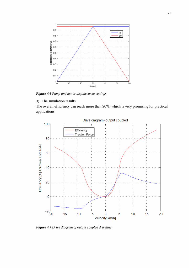
Figure 4.6 Pump and motor displacement settings
3) The simulation results
The overall efficiency can reach more than 90%, which is very promising for practical
applications.
Figure 4.7 Drive diagram of output coupled driveline
Page 33
24
Figure 4.8 Power transmission diagram of output driveline
Figure 4.7 shows the drive diagram of the output coupled circuit, and Figure 4.8 shows
the power distribution diagram of the output coupled circuit. Hydrostatic power portion
is 100 % in the starting point, but zero at the top speeds of the ranges. It can be seen
from the diagrams that with the decrease of the portion of hydrostatic transmission, the
overall efficiency keeps increasing, however the traction force decrease too, so the
portion of hydrostatic transmission should be controlled according to the actual
situation. In practical applications additional gear trains are used to increase the output
speed.
Page 34
25
4.3 Summary
This chapter studied the steady-state characteristics of input and output coupled circuits,
the simulation results show that both the advantages and disadvantages of input and
output coupled circuits. Input coupled circuits are mainly used in one direction drive.
The main advantage of input coupled circuit is its simplicity to be propagated to multi
stage transmissions. The main advantages of output coupled circuits are the good
transmission property in both drive direction, and the good efficiency it offers in a wide
range of transmission rate.
The lockup point is the point at which a power split CVT transmission becomes
purely mechanical, with the ring gear being stationary. The transmission ratio in this
situation is known as the lockup ratio. When designing a power split CVT transmission,
the first step is to analyze the planetary gear train to achieve the lockup ratio, once the
lockup ratio is known the whole transmission ratio can be calculated using it. The
benefits of the lockup point should be considered in practical engineering application,
this point is favorable for heavy duty working speed. Once the lockup point ratio is
known, the power distribution at any given time can be determined.
Page 35
26
5 HMPS-CVT Application
In the era of increasing fuel economy and reducing environment pollution, the
development of vehicle with new environment friendly and high efficient proposition
system becomes a necessity. Hybrid vehicles are one of the means to realize the goal.
This chapter reviews the current application of hydrostatic-mechanical power split CVT
in working machines, to provide information of the ways how the concept of basic
circuits of hydrostatic-mechanical power split CVT configure into real system and their
corresponding performance.
5.1 The Claas-Jarchow HM-8 and HM-II
Claas carried out a great amount of pioneering works since the late 1980s, which
resulting in the concepts Claas HM-8 (about 140 kW) and the later larger Claas HM-II,
also known as Traxion (about 220 kW). Both of the concepts were based on a patent of
Jarchow (Jarchow 1981), and they have been developed for the Claas carrier tractor
Xerion. The HM-8 had 7 power split ranges so that to keep the hydrostatic power
portion low and efficiency high. One creeper range works direct. The resulting tractors
was produced since 1996, while the HM-II (Traxion) with 5 power split ranges, one
direct and a conventional power shift reverser by clutches was presented at Agritechnica
1999 (Renius, K. Th., Resch, R. 2005). Both types were produced at limited production
volume. The Claas-Jarchow approach is characterized by an input coupled four-shaft
compound planetary which consists of two standard planetaries (Jarchow 1981). The
shifts between the ranges are done at synchronous speeds with dog clutches and the
power is handed over without any power interruption in a very short time, in which the
ratio is kept constant (no acceleration/deceleration of the vehicle). This principle is very
difficult to realize but does not need friction clutches (reduced costs, idling, losses).
However, a high sophisticated electronic control system is required. The measured
Claas HM-8 efficiencies have been found to be quite good which can cover the target of
the diagram.
Page 36
27
Figure 5.1 Efficiency target for CVT of larger tractors above 100kW (Renius 1999)
5.2 The Fendt Vario
Fendt equipped the Fendt tractor 926 Vario (191 kW) with its new, infinitely variable
Vario transmission at Agritechnica 1995. The scheme is shown in Fig. 5.2. It became
the worldwide first in series produced power split transmission for standard tractors
(1996). Its principle was soon expanded to more and more other Fendt models families.
At the end of 2004 four tractor families 400, 700, 800 and 900 were in production with
the Vario CVT as standard transmission.
Figure 5.2 Fent Vario for the tractor Favorit (1996)
The Fendt Vario is output-coupled power split CVT. The structure is based on a
principle of Molly (Renius, K. Th. and Resch, R. 2005). Basic development had been
done by the Fendt engineer H. Marschall (Marschall, H. 1973), who got several patents
Page 37
28
on it. In the forward direction, power is split by the planetary gear transmission and
merged by the shaft of the two hydrostatic units (Dziuba and Honzek 1997). The basic
power characteristics follow Fig. 5.3 and 5.4. Hydrostatic power portion is 100 % in the
starting point, but zero at the top speeds of the ranges.
Figure 5.3 Transmission characteristics of input coupled (Renius, K. Th. and Resch, R. 2005)
Figure 5.4 Transmission characteristics (Renius, K. Th. and Resch, R. 2005)
The power split unit covers two ranges: range L, which covers speeds up to 32
km/h, and range H which up to 50 km/h. The top speeds are nears the lock-up points.
The speed range beyond the lock-up range is not used to avoid power circulating, thus
there is no reversed hydrostatic power. An automatic shift on-the-go was introduced to
allow finger tip range selection within a speed band up to 20 km/h. The shift is done by
active synchronization support of the CVT. This is quite useful for heavy transports on
Page 38
29
hilly roads. The power interruption is quite small that mostly not realized by the driver.
For light duty transports, range H is sufficient for all speeds from zero to 50 km/h.
The required maximum hydrostatic power for the Fendt concept is very high, which
results in large units. Because commercially available variable axial piston pumps and
motors could not meet the efficiency requirements as shown in Figure 5.1, Fendt
developed its own 45 degree variable bent axis units, which offer in their best points
efficiencies of 95-96 % (swash plate units rather 89-92 %). A serious problem of the
Fendt concept was the high noise level due to the large units.
5.3 The Steyr S-Matic for Steyr, Case, New Holland
The Steyr S-Matic had been developed within the 1990s by the Austrian company Steyr
Antriebstechnik (SAT) which was later taken over by Zahnradfabrik Passau GmbH in
2000. The first concept became public in 1994, and series production was announced
with a modified structure (Zbigniew Żebrowski 2007) and realized early 2000 for the
standard tractors Steyr CVT and the Case CVX (both 88-125 kW). The transmission
was also adopted by New Holland TVT tractor series (2004), and McCormick
introduced it to a new tractor series VTX in 2005/2006.
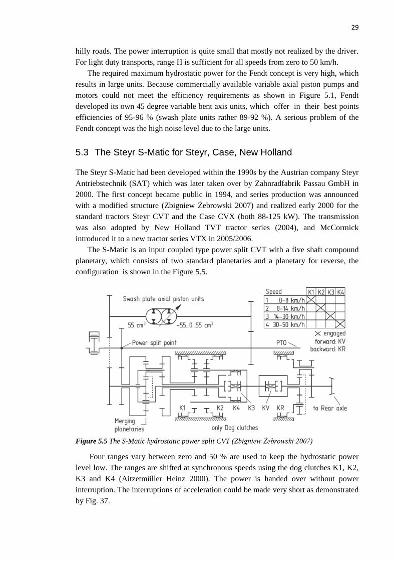
The S-Matic is an input coupled type power split CVT with a five shaft compound
planetary, which consists of two standard planetaries and a planetary for reverse, the
configuration is shown in the Figure 5.5.
Figure 5.5 The S-Matic hydrostatic power split CVT (Zbigniew Żebrowski 2007)
Four ranges vary between zero and 50 % are used to keep the hydrostatic power
level low. The ranges are shifted at synchronous speeds using the dog clutches K1, K2,
K3 and K4 (Aitzetmüller Heinz 2000). The power is handed over without power
interruption. The interruptions of acceleration could be made very short as demonstrated
by Fig. 37.
Page 39
30
Figure 5.6 Tractor drive diagram (Zbigniew Żebrowski 2007)
Efficiencies of the S-Matic have been published by Leitner et al. (2000) excluding
axles, which is shown in Figure 5.7.
Figure 5.7 Efficiency diagram (Aitzetmüller Heinz 2000)
5.4 The ZF Eccom for Deutz-Fahr, John Deere, Claas
ZF Eccom was first announced by ZF/ZP at Agritechnica 97. The configuration of ZF
Eccom is like:
Page 40
31
Figure 5.8 ZF - Eccom hydrostatic-mechanical power split CVT (Zbigniew Żebrowski 2007 )
There are three transmission families within ZF-Eccom: 1) Eccom 1.5 (110kW); 2)
Eccom 1.8 (130kW); 3) Eccom 3.0 (220kW). Deutz-Fahr was the first tractor company
using the Eccom (version1.5) in its new series Agrotron TTV (92/103/110 kW). John
Deere applies the Eccom since 2001 for its 6000 tractor line known as AutoPowr. Claas
has announced to use the Eccom 3.0 for its new Xerion carrier tractor family.
The concept of the power split system is a type of input coupled circuit. The four
ranges concept keeps the hydrostatic power in a low level. Figure below illustrates the
linear output speed variation of the hydrostatic unit between minus 2300 and plus 2300
rpm crossing at zero the lockup point (Zbigniew Żebrowski 2007).
Page 41
32
Figure 5.9 Hydrostatic power portions and speed of first left sun gear within the 4 ranges
(Pohlenz and Gruhle 2002)
Two planetaries are used, the first of which is a five-shaft compound planetary that
combines three standard planetaries, the second of which is a standard planetary. This
compound planetary produces 3 ranges using friction clutches K1, K2 and K3, while the
standard planetary produces the fourth range K4. Forward and reverse shift is realized
by using two conventional reverser clutches KV, KR. The clutch dimensions are large
due to the high possible slipping speeds. Efficiencies of this transmission are published
excluding the axles (Renius, K. Th., Resch, R.).
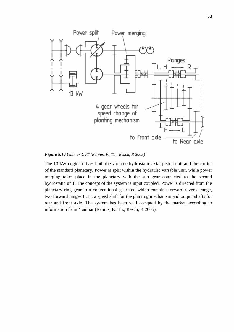
5.5 Yanmar CVT
Yanmar Agricultural Equipment Co., Ltd., Japan, produced a self propelled rice
transplanter in series since 2002 which applies a power split CVT for the vehicle drive.
Figure 5.9 shows the concept of Yanmar CVT.
Page 42
33
Figure 5.10 Yanmar CVT (Renius, K. Th., Resch, R 2005)
The 13 kW engine drives both the variable hydrostatic axial piston unit and the carrier
of the standard planetary. Power is split within the hydraulic variable unit, while power
merging takes place in the planetary with the sun gear connected to the second
hydrostatic unit. The concept of the system is input coupled. Power is directed from the
planetary ring gear to a conventional gearbox, which contains forward-reverse range,
two forward ranges L, H, a speed shift for the planting mechanism and output shafts for
rear and front axle. The system has been well accepted by the market according to
information from Yanmar (Renius, K. Th., Resch, R 2005).
Page 43
34
5.6 Summary
The hydrostatic-mechanical power split CVT is a special type of power split CVT,
which is suitable for high power density application. The hydrostatic-mechanical power
split CVT is not a newly developed technology, Renault (Pablo Noben 2007), derived a
famous idea to use the principle of internal hydrostatic-mechanical power split for a
passenger car gearbox. The presence of this type of transmission has been increasing
ever since its emergence. However, only a handful of mobile machines make use of
hydrostatic-mechanical power split CVT. Its potential is far from fully explored. This
chapter reviews five concepts of hydrostatic-mechanical power split CVT
configurations that commercially developed for larger tractors to give an idea on the
practical application of this type of transmission technology and their actual
performances, all the concepts demonstrate good properties, four of them could enter
series-production stage. Power split CVT provides better system efficiency over the
traditional hydrostatic CVT mode, there are great potential markets to be explored in the
future.
Page 44
35
6 Suitability study
This chapter studies the suitability of hydrostatic-mechanical power split CVT
technology, the studies include working cycle suitability and power range suitability.
The studies aimed to find suitable working conditions for the hydrostatic-mechanical
power split CVT, under which it demonstrates good efficiency.
6.1 Diesel engine
The diesel engine model made by Daiheng Ni (Daiheng Ni 2008) was used in this study,
since this model was proved simple and stable. It makes use of the maximum engine
power and maximum engine torque and related angular velocities , ,
all these parameters can be found from the specification of an engine. The approximate
torque curve is:
(65)
where and are constants, and is the engine speed at peak torque. To ensure
that the power curve peaks at , is replaced with a different coefficient as:
(66)
Give that the engine outputs at and output at , the following
equations can be derived:
(67)
(68)
(69)
Solve the equations:
(70)
(71)
Therefore
(72)
(73)
Page 45
36
According to Daiheng Ni the validation curves of the model are shown in Figure 6.1,
6.2, the model used in this study is model two.
Figure 6.1 Engine power curve (Daiheng Ni 2008)
Figure 6.2 Engine power curve (Daiheng Ni 2008)
6.2 Model of hydrostatic transmission
The following assumptions were made for modeling the hydrostatic transmission
a) Temperature was assumed to be constant,
Page 46
37
b) Pressure drop and fluid dynamics between pump and motor were ignored,
c) Low pressure was assumed constant,
d) No internal or external leakages between pump and motor.
The pump flow is
(74)
is the leakage flow of the pump, and it is defined as
(75)
The motor flow is
(76)
is the leakage flow of the motor, and it is defined as
(77)
The system continuity equation is
(78)
The motor torque is
(79)
is the hydro-mechanical torque loss of the motor, defined as
(80)
The pump torque is
(81)
is the hydro-mechanical torque loss of the pump, defined as
(82)
The oil bulk modulus B = 1500Mpa. The pump and motor model can be found in
Appendix I and J, the hydrostatic transmission path can be found in Appendix K. Based
on the equations of above the dynamic model of the hydrostatic transmission is derived
as shown in Figure 6.3.
Page 47
38
Figure 6.3 Dynamic model of the hydrostatic transmission
6.3 Tire road connection
The slip between tire and road was expressed according to the formula derived by
Gustafsson (Gustafsson 1997) as
(83)
Here is the circumferential velocity of the tire, which is expressed as ,
and is the absolute velocity.
The friction coefficient is defined based as a function of the traction force and the
normal force :
(84)
(85)
To apply to both positive and negative velocities, the equation was modified as follows:
(86)
is a constant to prevent division by zero crossing.
6.4 Drive wheel model
Figure 6.4 shows the drive wheel model.
Page 48
39
Figure 6.4 Drive wheel illustration
is the traction force
is the drive torque
is the friction torque that is a function of the wheel angular velocity and the
constant coulomb friction torque
(87)
The driving wheel torque equation can be written as follows
(88)
6.5 Vehicle dynamics
The vehicle dynamics is illustrated in Figure 6.5
Page 49
40
Figure 6.5 vehicle dynamics
The fraction force of the vehicle is expressed as a function of the velocity
(89)
The vehicle force equation can be written as
(90)
Here is the external load force, is the vehicle mass.
6.6 Powertrain model
The powertrain model calculates the velocity of the vehicle according to the desired
speed of the engine and the pump displacement setting , the hydraulic motor
angular velocity is defined as a function of and . The power train model was
based on the simulation model of Huhtala (1996).
(91)
The drive torque is the output torque multiplied by the gear ratio between
output shaft and the drive wheel :
(92)
The accessory torque is a function of the engine speed, it can be written as:
(93)
The engine produces output torque according to the summation of the mechanically
transmitted torque , the hydrostatic unit driven torque which is the pump torque
multiplied by the gear ratio , and the torque that consumed by the accessory
devices, which consist of control and flushing pump. The following diagram shows the
dynamic model of the hydrostatic-mechanical power split CVT. The details of final can
Page 50
41
be found in Appendix E, the engine model can be found in Appendix F, the accessory
and planetary gear model can be found in Appendix G and H.
Figure 6.6 Powertrain model
6.7 The powertrain simulation examples
1) The response of the powertrain model to hydrostatic units control signal
Table 6.1 Powertrain simulation parameters
Simulation parameters
Engine speed Constant at 2000rpm
Load 5000N
Pump displacement setting Changes from 0.25 to 1, then to 0.6
Page 51
42
Figure 6.7 Pump displacement setting
Figure 6.8 Vehicle velocity response
2) The response of the powertrain model to engine control signal
Table 6.2 Powertrain control parameters
Simulation parameters
Engine speed Changes from 1625rpm to 1997rpm then to 1800rpm
Page 52
43
Load 5000N
Pump control Constant at 1
Figure 6.9 Engine speed control signal
Figure 6.10 Vehicle velocity response
6.8 The working cycle suitability
This study is aimed to find a suitable working cycle under which the hydrostatic-
mechanical power split CVT performs best, in other words, the efficiency of the whole
working cycle keeps at an high level that can save considerable amount of energy. The
typical hybrid vehicle working principle is shown as (Hanyun Yang 2009):
Page 53
44
Figure 6.11 Typical hybrid vehicle working cycle
According to the typical hybrid vehicle working principle of Eaton hybrid solution, the
working cycle studied here defined as
Figure 6.12 Powertrain simulation working cycle
The simulation parameters of the working cycle study are chosen as
Table 6.3 Working cycle simulation parameters
Simulation parameters
Engine speed 2000rpm
Load 5000N
Pump displacement setting 0.7510.7
The simulation result Figure 6.13 and Figure 6.14 show that the efficiency of the
transmission keeps higher than during the whole working cycle. The transmission
efficiency becomes higher when the portion of the hydrostatic transmission becomes
smaller, because at this case more energy is transmitted via mechanical path, which has
a higher efficiency than the hydrostatic path.
The accelerateuniform motiondecelerate working mode is widely used by many
kinds of transportations such as transit bus, excavator, truck, crane, etc. This means the
hydrostatic-mechanical power split CVT technology has great potential to be widely
adopted by working machines.
Page 54
45
Figure 6.13 Powertrain efficiency curve
Figure 6.14 Powertrain velocity response
According to Eaton (Brad Bohlmann 2007), a diesel hybrid hydraulic shuttle bus on a
Ford E450 chassis was delivered to the US Army in May 2006. The vehicle met or
Page 55
46
exceeded all of the program goals including demonstrating >25% fuel economy
improvement on the EPA city driving cycle and reducing in-cab noise during
acceleration by more than six dBA. Another Eaton solid waste compaction (refuse)
trucks showed the following performance:
Table 6.4 Eaton vehicle performance
Economy Mode Productivity Mode
Fuel economy improvement 28% 17%
Vehicle Acceleration +2% +26%
Productivity N/A +11.5%
Brake Life >2x >2x
6.9 The power range suitability study
Hydrostatic-mechanical power split CVT systems have much higher power capabilities,
in addition to the higher transmission efficiency, they typically regenerate much more
braking energy than traditional transmission systems. According to Eaton (Brad
Bohlmann 2007), a series hybrid hydraulic UPS truck demonstrated 50-70% better fuel
economy than a standard truck.
This study aimed to find the power range suitability of the hydrostatic-mechanical
power split CVT technology, power range suitability shows the relationship between
engine power range and the total efficiency of the transmission. The power range in this
study is 30kW to 120kW. The following table and figure show the simulation result.
Table 6.5 Transmission suitability study result
Engine speed 1600rmp
Hydraulic unit volumetric efficiency 0.88
Hydraulic unit hydraulic-mechanical
efficiency
0.88
Engine power ( ) Torque ( ) Efficiency( )
30 178.6 83.22
35 208.9 84.4
40 238.7 85.83
45 268.5 87.4
50 298.3 87.73
55 328.7 88.83
60 358.3 89.33
65 387.2 89.77
70 417.8 90.17
75 447.5 90.51
80 477.2 90.78
Page 56
47
85 507.2 91.11
90 536.8 91.3
95 566.9 91.5
100 596.5 91.65
105 626.5 91.9
110 656.3 92.04
115 686.3 92.16
120 715.6 92.25
Figure 6.15 Power range suitability curve
The study shows that the higher the power is applied to the transmission, the better
efficiency can be achieved. This means that hydrostatic-mechanical power split CVT
technology can be used in most segments of the working machine market, including all
light, medium and heavy duty passenger cars, city buses, and delivery trucks. Great
potential for application in hybrid technology still remains, the market is still evaluating
the technology in many cases.
Page 57
48
6.10 Conclusion
This study builds a dynamic power-train model of output coupled hydrostatic-
mechanical power split CVT. Based on analysis, a normally used working cycle:
accelerate-uniform motion-decelerate was chose to test the efficiency of the power-
train model to test the suitability, the simulation result shows excellent efficiency, this
shows hydrostatic-mechanical power split CVT is suitable for machines operate under
that working cycle. Then a power-range suitability test carried out based on simulation,
the result shows that within the range from 30kW to 120kW, the higher the engine
power, the better efficiency is offered by the transmission system, the results shows that
hydrostatic-mechanical power split CVT is especially for medium and heavy duty
working machines.
In addition, the study result shows that hydrostatic-mechanical power split CVT
technology is able to increase the whole system efficiency over that of a signal
hydrostatic CVT mode. However, power CVT is difficult to cover the full-required
speed range, therefore in practical application additional range gears are needed to
increase the speed range.
Page 58
49
7 Summary
In this study, two general hydrostatic-mechanical power split CVT configurations: input
and output coupled hydrostatic-mechanical power split CVT were studied to investigate
power split transmission, including the power distribution, the static models, and the
steady-state characteristics, to find the advantages and disadvantages of both circuits.
Then current applications of the hydrostatic-mechanical power split CVT technology
were reviewed to give an idea of how the concept was being used in real product
application, and to reveal that there is still great market potential to be explored. Finally,
a suitability study was made to show under which working cycle the hydrostatic-
mechanical power split CVT offers the best, and under which engine power range the
transmission performs best.
The study shows that the lockup point is very important for a power split CVT, the
benefits of the lockup point should be considered in practical application to make full
use the benefits, for example in heavy duty working speed (6-12km/h). Both principles:
input coupled and output coupled systems have advantages and disadvantages, both of
them suitable for different applications, so both of the principles are of interesting in
practical engineering applications. Overall, hydrostatic-mechanical power split provides
better efficiency over traditional hydrostatic CVT, though the design of hydrostatic-
mechanical power split CVT is more complex than the traditional hydrostatic CVT.
Hydrostatic-mechanical power split CVT is quite suitable for the heavy duty working
machines with frequent accelerate and decelerate operations, the higher the power
density the better efficiency it will provide.
All the studies were carried out theoretically, practical applications are different
from theoretical study results, it is recommend that in real product design a combination
of theoretical study and practical test is necessary.
Page 59
50
References
Aitzetmüller Heinz. Steyr S-Matic – The Future CVT System. Seoul 2000 FISITA
World Automotive Congress. 2000
Brad Bohlmann. Hybrid Hydraulic System Development for Commercial Vehicles.
[WWW]. [Cited 01/09/2010]. Available at:
http://www.aqmd.gov/tao/conferencesworkshops/HydraulicHybridForum/BohlmannSli
des.pdf
Daiheng Ni., Dwayne Henclewood. Simple Engine Models for VII-Enabled In-Vehicle
Applications. IEEE TRANSACTIONS ON VEHICULAR TECHNOLOGY, VOL. 57,
NO. 5, SEPTEMBER 2008.
Dziuba, F. and R. Honzek. Neues stufenloses leistungsverzweigtes Traktorgetriebe. (A
new power-split transmission). Agrartechnische Forschung Vol. 3 No.1: 19-27.1997.
Erkkilä M., Model-based design of power-split drivelines. Doctoral dissertation.
Tampere University of Technology publication 825. 2009
Gustafsson, F. Slip-based tire-road friction estimation, Automatica Vol. 33 No.6, 1997,
pp.1087-1099.
Hanyun Yang. Eaton Hybrid Solutions: Bus Applications. [WWW]. [Cited 01/09/2010].
Available at: http://www.modern.ipacv.ro/Eaton%20Hybrid%20Solutions-
%20COMPRO%20Final.pdf
Heera Lee, Hyunsoo Kim. CVT Ratio Control for Improvement of Fuel Economy by
Considering Powertrain Response Lag. KSME International Journal VoL 17 No. 11, pp.
1725~1731, 2003.
Huhtala, K. Modeling of the hydrostatic transmission – steady state, linear and non-
linear models. Doctoral dissertation. Acta Polytechnica Scandinavia mechanical
engineering series No.123, Helsinki, 1996.
Ivantysynova Monika. Design and Modeling of Fluid Power Systems ME 597/ABE 591
-Lecture 15. [WWW]. [Cited 01/07/2010]. Available at:
https://engineering.purdue.edu/Maha/docs/Courses/me597-abe591/Fall2007/ME597-
lecture15-07.pdf
Ivantysynova Monika. Power split drive technology – trends & requirements.
Developments in fluid power control of Machinery and Manipulators, 2nd International
Scientific Forum, Cracow, Poland 28 June – 2 July 2000.
Jarchow, F. 1981. Hydrostatischmechanisches Stellkoppelgetriebe mit eingangsseitiger
Leistungsverzweigung (Infinitely variable hydromechanical couple transmission with
Page 60
51
power split at input) German Patent No. 3 147 447 C2. Filed 1.12.1981, granted
14.06.1984.
Kress JH. Hydrostatic power-splitting transmissions for wheeled vehicles -
Classification and theory of operation. SAE Paper No. 680549; 1968.
Kevin R. Lang. Continuously Variable Transmissions An Overview of CVT Research
Past, Present, and Future. [WWW]. [Cited 01/09/2010]. Available at:
http://www.lasercannon.com/Murano/Files/cvt.pdf
Marschall, H. 1973. Antriebsvorrichtung, insbesondere fürland- und bauwirtschaftlich
genutzte Fahrzeuge (Drive concept, mainly for agricultural and construction vehicles).
German patent 2 335 629, filed 13.7.1973, granted 30.1.1975.
Molly, H. Hydrostatische Fahrzeugantriebe – ihre Schaltung und konstruktive
Gestaltung. Teil I und II. (Hydrostatic vehicle drives - their control and engineering.
Part I and II). ATZ Automobiltechnische Zeitschrift Vol. 68, No. 4: 103-110 (I) and No.
10: 339-346 (II). Morris, W.H.M. 1967. The IHC Hydrostatic.).1966.
Norman H. Beachley., Andrew A. Frank. Continuously variable transmissions: theory
and practice. College of Engineering, University of Wisconsin, Madison. 1979.
P. Linares., V. Méndez., H. Catalán. Design parameters for continuously variable
power-split transmissions using planetary with 3 active shafts. Journal of
Terramechanics
Volume 47, Issue 5, Pages 323-335, October 2010.
Pohlenz, J. and W.-D. Gruhle. Stufenloses hydrostatisch-mechanisch
leistungsverzweigtes Getriebe (Continuously variable hydro-mechanical power split
transmision). O+P Ölhydraulik und Pneumatik Vol. 46, No. 3: 154-158. 2002
Pablo Noben. A comparison study between power-split CVTs and a push-belt CVT.
Technische Universiteit Eindhoven. 2007
Renius, K. Th., Resch, R. Continuously variable tractor transmission. American Society
of Agricultural and Biological Engineers, St. Joseph, Michigan, USA 2005, pp.5-37
Renius, K. Th. Tractors. Two Axle Tractors. In: CIGR Handbook of Agricultural
Engineering. Vol. III, Plant Production Engineering (edited by B.A. Stout and B.
Cheze):115-184.1999.
Thoma J., Hydrostatic power transmission, Morden UK, Trade and Technical Press,
1964.
Yuliang Leon Zhou. Modeling and Simulation of Hybrid Electric Vehicles. University
of Science and Technology Beijing. 2005
Page 61
52
Zbigniew Żebrowski. Hybrid Gears in Farm Tractors. TEKA Kom. Mot. Energ. Roln. -
OL PAN, 2007, 7, 321–334
Page 62
53
Appendix: Simulink models
A. Steady-state ump model
B. Steady-state motor model
Page 63
54
C. Input coupled steady state model
D. Output coupled steady state model
Page 64
55
E. Final drive
F. Engine model
Page 65
56
G. Accessory model
H. Planetary gear model
Page 66
57
I. Dynamic pump model
J. Dynamic motor model
Page 67
58
K. Hydrostatic transmission part