Chirality in the ¹3⁶Nd and ¹3⁵Nd nuclei - Accueil - TEL

HAL Id: tel-02347000https://tel.archives-ouvertes.fr/tel-02347000

Submitted on 5 Nov 2019

HAL is a multi-disciplinary open accessarchive for the deposit and dissemination of sci-entific research documents, whether they are pub-lished or not. The documents may come fromteaching and research institutions in France orabroad, or from public or private research centers.

L’archive ouverte pluridisciplinaire HAL, estdestinée au dépôt et à la diffusion de documentsscientifiques de niveau recherche, publiés ou non,émanant des établissements d’enseignement et derecherche français ou étrangers, des laboratoirespublics ou privés.

Chirality in the ¹3�Nd and ¹3�Nd nucleiBingfeng Lv

To cite this version:Bingfeng Lv. Chirality in the ¹3�Nd and ¹3�Nd nuclei. Nuclear Experiment [nucl-ex]. Université ParisSaclay (COmUE), 2019. English. �NNT : 2019SACLS353�. �tel-02347000�

https://tel.archives-ouvertes.fr/tel-02347000

https://hal.archives-ouvertes.fr

NN

T:2

019S

ACLS

353

Chirality in the 136Nd and 135Nd nucleiThese de doctorat de l’Universite Paris-Saclay

preparee a l’Universite Paris-Sud

Ecole doctorale n�576 particules hadrons energie et noyau: instrumentation, image,cosmos et simulation (PHENIICS)

Specialite de doctorat : Structure et reactions nucleaires

These presentee et soutenue a Orsay, le 11 octobre 2019, par

BINGFENG LV

Composition du Jury :

MME AMEL KORICHIDirectrice de Recherche, CSNSM PresidenteMME ELENA LAWRIEProfesseure associee, iThemba Labs, South Africa RapporteurMME NADINE REDONDirectrice de Recherche, IP2I Lyon RapporteurM. ZHONG LIUProfesseur des Universites, Chinese Academy of Sciences, IMP, China ExaminateurM. COSTEL PETRACHEProfesseur des Universites, Paris-Sud/Paris Saclay Directeur de these

2

Acknowledgements

I would like to express my sincere gratitude to those who helped me and shared their ex-periences during my PhD. The work presented here would have been impossible to concludewithout their guidance and assistance.

First and foremost, I would like to express my sincere gratitude to my supervisor Pro-fessor Costel Petrache, for his systematic teaching and training me in experimental nuclearstructure research. It is my great honor to have a supervisor who is so famous and highlyrespected in the nuclear physics. Also, I want to express my deepest grateful to him for histake care of me, and all the things he has done for me even if he never told me. In addition,for sure, his personal qualities, like work hard, great passion for research, explorative spirit......, will influence me more in the future. For me, he is not only a mentor in my work, butalso in my life.

I would like to also thank my CSNSM colleagues. Alain Astier help will never be for-gotten due to his selfless shared many data analysis skills used in present work. I feel verylucky that I had a very nice officemate, Etienne Dupont, who assisted me a lot in my dailylife in France. I want to say "Merci beaucoup, monsieur Etienne Dupont ". I also would liketo thank Amel Korichi, Araceli Lopez-Martens, Jérémie Jacob, Nicolas Dosme and all theother colleagues in CSNSM for their assistance.

I also thank the nuclear structure group of IMP, Lanzhou, in particular, Xiaohong Zhou,my supervisor, also Guo Song and Jianguo Wang for initiating me in experimental nuclearphysics research. In particular, I would like to thank Dr. Guo Song for establishing the colla-boration between Professor Costel Petrache group and the nuclear structure group in IMP,which provided me the opportunity to do my PhD in CSNSM, Orsay, France.

I also would like to thank another one of my supervisors, Wenhui Long from LanzhouUniversity for his continue support and very wisdom advice for my future career.

I would like to thank all our collaborators, in particular to Prof. Meng Jie and Dr. QiboChen for their excellent theoretical work made for the interpretation of the present data.

I am thankful to the jury members of my PhD defense, Dr. Amel Korichi (CSNSM, Or-say), Dr. Elena Lawrie (iThemba Labs, South Africa), Dr. Nadine Redon (IP2I Lyon), andDr. Zhong Liu (IMP, Lanzhou) for having spent their valuable time to evaluate my PhDwork and read my thesis, also to give suggestions and comments on my manuscript.

I would like to also thank the financial support of China Scholarship Council (CSC) andCSNSM, CNRS.

Finally, I would like to express my heartfelt gratitude to my parents for their love, careand constant spiritual support in my 22 years student career. Also, thanks to my girl friendCui Xiaoyun for her understanding, accompany and endless encouragement.

3

Contents

Acknowledgements 3

1 Introduction 171.1 Chirality . . . . . . . . . . . . . . . . . . . . . . . . . . . . . . 18

1.1.1 Nuclear Chirality . . . . . . . . . . . . . . . . . . . . . 191.1.2 Multiple chiral doublets (M�D) . . . . . . . . . . . . . 20

1.2 Fingerprints of the chiral bands . . . . . . . . . . . . . . . . . 211.2.1 Energy spectra . . . . . . . . . . . . . . . . . . . . . . 211.2.2 Electromagnetic transitions rates . . . . . . . . . . . . 211.2.3 Other fingerprints . . . . . . . . . . . . . . . . . . . . . 22

1.3 Motivation of this study . . . . . . . . . . . . . . . . . . . . . 231.4 Outline of thesis . . . . . . . . . . . . . . . . . . . . . . . . . . 23

2 Theoretical backgroud 252.1 Liquid drop model . . . . . . . . . . . . . . . . . . . . . . . . 252.2 The shell model . . . . . . . . . . . . . . . . . . . . . . . . . . 262.3 The deformed shell model . . . . . . . . . . . . . . . . . . . . 28

2.3.1 Deformed parameters . . . . . . . . . . . . . . . . . . . 282.3.2 The Nilsson model . . . . . . . . . . . . . . . . . . . . 32

2.4 Particle-rotor model . . . . . . . . . . . . . . . . . . . . . . . 372.4.1 Strong coupling . . . . . . . . . . . . . . . . . . . . . . 382.4.2 The decoupling limit . . . . . . . . . . . . . . . . . . . 382.4.3 Four-j shells particle-rotor model . . . . . . . . . . . . 39

2.5 Cranked Nilsson-Strutinsky model . . . . . . . . . . . . . . . . 412.5.1 Cranking model . . . . . . . . . . . . . . . . . . . . . . 412.5.2 The rotating liquid drop model . . . . . . . . . . . . . 452.5.3 The configuration-dependent CNS approach . . . . . . 46

2.6 Tilted axis cranking covariant density functional theory . . . 472.6.1 Tilted axis cranking . . . . . . . . . . . . . . . . . . . 472.6.2 TAC-CDFT . . . . . . . . . . . . . . . . . . . . . . . . 50

2.7 Transition probabilities . . . . . . . . . . . . . . . . . . . . . . 52

5

6 CONTENTS

3 Experimental techniques 533.1 Heavy-ion fusion-evaporation reactions . . . . . . . . . . . . . 533.2 Interaction mechanisms of the �-rays with matter . . . . . . . 55

3.2.1 Photoelectric absorption . . . . . . . . . . . . . . . . . 553.2.2 Compton scattering . . . . . . . . . . . . . . . . . . . . 553.2.3 Pair production . . . . . . . . . . . . . . . . . . . . . . 56

3.3 High-purity Germanium �-ray detector . . . . . . . . . . . . . 563.4 The JUROGAM II array . . . . . . . . . . . . . . . . . . . . . 583.5 The RITU gas-filled recoil separator . . . . . . . . . . . . . . . 593.6 The GREAT spectrometer . . . . . . . . . . . . . . . . . . . . 613.7 Total-Data Readout (TDR) . . . . . . . . . . . . . . . . . . . 62

4 Experimental details and processing of the data 654.1 Experimental details . . . . . . . . . . . . . . . . . . . . . . . 654.2 Data processing . . . . . . . . . . . . . . . . . . . . . . . . . . 65

4.2.1 Energy calibrations and gain matching . . . . . . . . . 654.2.2 Efficiency calibrations for Ge detectors . . . . . . . . . 664.2.3 Doppler shift correction . . . . . . . . . . . . . . . . . 674.2.4 Add-back for the clover detectors . . . . . . . . . . . . 674.2.5 Spin and parity assignments . . . . . . . . . . . . . . . 68

5 Towards complete spectroscopy of 136Nd 715.1 Experimental results and level scheme . . . . . . . . . . . . . . 71

5.1.1 The low-spin � band and bands N1, N2 . . . . . . . . . 725.1.2 The medium-spin bands L and T . . . . . . . . . . . . 735.1.3 The dipole bands . . . . . . . . . . . . . . . . . . . . . 755.1.4 The highly-deformed bands . . . . . . . . . . . . . . . 81

5.2 Discussion . . . . . . . . . . . . . . . . . . . . . . . . . . . . . 985.2.1 M�D interpretation of the chiral bands within TAC-

CDFT framework . . . . . . . . . . . . . . . . . . . . . 985.2.2 M�D interpretation of the chiral bands within PRM

framework . . . . . . . . . . . . . . . . . . . . . . . . . 1035.2.3 CNS interpretation of all rotational bands . . . . . . . 108

6 Evidence of M�D in the odd-A nucleus 135Nd 1236.1 Introdution . . . . . . . . . . . . . . . . . . . . . . . . . . . . 1236.2 Experimental results and level scheme . . . . . . . . . . . . . . 1246.3 Discussion . . . . . . . . . . . . . . . . . . . . . . . . . . . . . 127

7 Search for long-lived isomeric states 1397.1 Introduction . . . . . . . . . . . . . . . . . . . . . . . . . . . . 1397.2 The recoil-decay tagging technique . . . . . . . . . . . . . . . 1397.3 Results of the focal plane . . . . . . . . . . . . . . . . . . . . . 140

CONTENTS 7

Synthèse 145

Conclusions and Outlook 147

Appendix A JUROGAM II detector angles 149

8 CONTENTS

List of Figures

1.1 Left- and right-handed chiral systems for a triaxial odd-oddnucleus. The symbols ~J , ~R, ~j⌫ , and ~j⇡ denote respectively thetotal angular momentum, the angular momenta of the core,of the neutron and of the proton, respectively. Figure adoptedfrom Ref. [1]. . . . . . . . . . . . . . . . . . . . . . . . . . . . 19

1.2 The nuclides with chiral doublet bands (red circles) and M�D(blue pentagons) observed in the nuclear chart. The black squaresrepresent stable nuclides. Figure adopted from Ref. [2]. . . . . 22

2.1 Schematic nuclear levels calculated by the shell model includingthe l2 and ~l · ~s terms. Figure adapted from Ref. [3]. . . . . . . 29

2.2 The lowest four vibrations of a nucleus. The dashed lines showthe spherical equilibrium shape and the solid lines show an in-stantaneous view of the vibrating surface. Figure adapted fromRef. [4]. . . . . . . . . . . . . . . . . . . . . . . . . . . . . . . 30

2.3 Plot of the Eq. 2.12, for k=1, 2, 3, corresponding to the increasein the axis lengths in the x, y, and z directions. Figure adoptedfrom Ref. [5]. . . . . . . . . . . . . . . . . . . . . . . . . . . . 31

2.4 Schematic of nuclear shapes with respect to the deformationparameters (�

2

, �), as defined in the Lund convention. Figureadapted from Ref. [6]. . . . . . . . . . . . . . . . . . . . . . . 32

2.5 Schematic of the quantum numbers which can describe the de-formed nucleus. ⇤, ⌦, ⌃, and K are the projections of the or-bital angular momentum l, of the total angular momentum ofthe particle j, of the spin of the particle s, and of the totalangular momentum J onto the symmetry axis, respectively. Inaddition, ~R is the angular momentum of the core and M is theprojection of the total angular momentum onto the laboratoryaxis. . . . . . . . . . . . . . . . . . . . . . . . . . . . . . . . . 34

2.6 Nilsson diagram for protons in the 50 Z 80 region showingthe single-particle energies as a function of the deformation pa-rameter ✏

2

. For ✏2

>0, corresponding to the prolate shape; for✏2

=0, corresponding to the spherical shape; for ✏2

< 0, corre-sponding to the prolate shape. Labels obey the ⌦⇡[Nnz⇤] rule. 35

9

10 LIST OF FIGURES

2.7 Nilsson diagram for neutrons in the 50 N 80 region show-ing the single-particle energies as a function of the deformationparameter ✏

2

. For ✏2

>0, corresponding to the prolate shape; for✏2

=0, corresponding to the spherical shape; for ✏2

< 0, corre-sponding to the prolate shape. Labels obey the ⌦⇡[Nnz⇤] rule. 36

2.8 Schematic diagram of the strong coupling limit in the particle-rotor model. . . . . . . . . . . . . . . . . . . . . . . . . . . . . 39

2.9 Schematic diagram of the decoupling limit in the particle-rotormodel. . . . . . . . . . . . . . . . . . . . . . . . . . . . . . . . 39

2.10 Discrete symmetries of the mean field of a rotating triaxial re-flection symmetric nucleus. The axis of rotation (z) is markedby the circular arrow. The rotational band structures associatedwith each symmetry type are presented on the right side. Thisfigure was taken from Ref. [7]. . . . . . . . . . . . . . . . . . . 49

3.1 Schematic illustration the heavy-ion fusion-evaporation reactionforming a compound nucleus and its decay. . . . . . . . . . . . 54

3.2 (a) Photoelectric absorption, (b) Compton scattering, (c) Pairproduction. . . . . . . . . . . . . . . . . . . . . . . . . . . . . 55

3.3 Reverse bias of the p-n junction. . . . . . . . . . . . . . . . . . 573.4 The schematic configuration of a BGO anti-Compton shield of

a HPGe detector. . . . . . . . . . . . . . . . . . . . . . . . . . 583.5 JUROGAM II array. . . . . . . . . . . . . . . . . . . . . . . . 593.6 Scheme of gas-filled recoil separator RITU. The figure is taken

from Ref. [8]. . . . . . . . . . . . . . . . . . . . . . . . . . . . 603.7 Schematic diagram of GREAT sepctrometer. . . . . . . . . . . 613.8 Schematic illustration of a typical RDT setup and the signal

times for each detector relative to the an event stamp in theDSSDs. This figure is adapted from Ref. [9]. . . . . . . . . . . 63

4.1 A sample of calibrated overlayed energy spectra of 152Eu forsome Ge detectors of the JUROGAM II array. The peaks cor-responding to the contaminating transitions are indicated withasterisks. . . . . . . . . . . . . . . . . . . . . . . . . . . . . . . 66

4.2 Geometry of the detector arrangement with the beam as orien-tation axis. . . . . . . . . . . . . . . . . . . . . . . . . . . . . 69

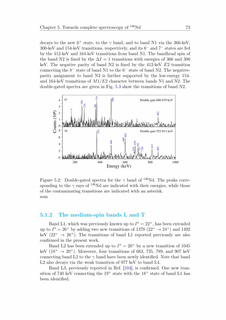
5.1 Partial level scheme of 136Nd showing the low- and medium-spinbands. . . . . . . . . . . . . . . . . . . . . . . . . . . . . . . . 72

5.2 Double-gated spectra for the � band of 136Nd. The peaks corre-sponding to the � rays of 136Nd are indicated with their energies,while those of the contaminating transitions are indicated withan asterisk. . . . . . . . . . . . . . . . . . . . . . . . . . . . . 73

LIST OF FIGURES 11

5.3 Double-gated spectra for the band N2 of 136Nd. The peaks cor-responding to the contaminating transitions are indicated withasterisks. . . . . . . . . . . . . . . . . . . . . . . . . . . . . . . 74

5.4 Double-gated spectrum for band L4 of 136Nd. . . . . . . . . . 745.5 Sum of spectra obtained by double-gating on all combinations

of in-band transitions of band T2. The peaks corresponding tothe contaminating transitions are indicated with asterisks. . . 75

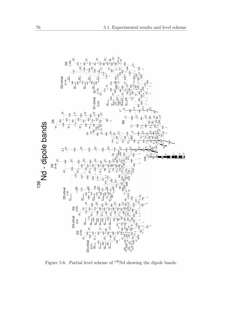
5.6 Partial level scheme of 136Nd showing the dipole bands. . . . . 765.7 a) Sum of spectra obtained by double-gating on all combina-

tions of the 220-, 254- and 294-keV transitions of band D1. b)Spectrum obtained by double-gating on the 220- and 254-keVtransitions of band D1. The peaks corresponding to the in-bandtransitions of band D1-chiral and to the connecting transitionsto band D1 are indicated with asterisks. . . . . . . . . . . . . 77

5.8 Spectra constructed by double-gating on transitions of band D2which shows the connecting transitions of band D2-chiral. Thetransitions marked with asterisks indicate low-lying transitionsin 136Nd. The red lines show how the connecting transitionsdisappear when gating on successive higher-lying transitions ofband D2. . . . . . . . . . . . . . . . . . . . . . . . . . . . . . . 78

5.9 Double-gated spectrum on the 249- and 345-keV transitions ofband D3, showing the connecting transitions of band D3-chiralto band D3, which are indicated with asterisks. . . . . . . . . 79

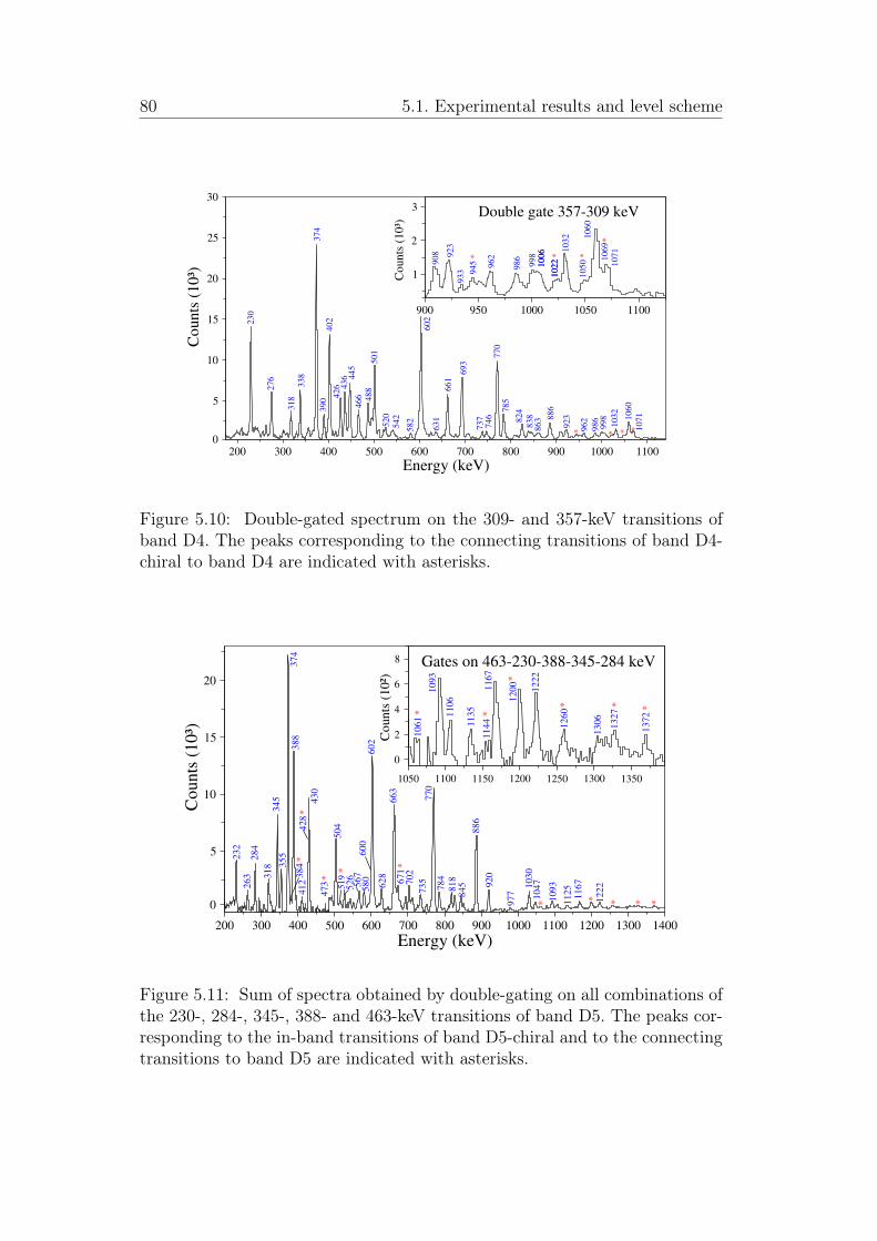
5.10 Double-gated spectrum on the 309- and 357-keV transitions ofband D4. The peaks corresponding to the connecting transitionsof band D4-chiral to band D4 are indicated with asterisks. . . 80

5.11 Sum of spectra obtained by double-gating on all combinationsof the 230-, 284-, 345-, 388- and 463-keV transitions of bandD5. The peaks corresponding to the in-band transitions of bandD5-chiral and to the connecting transitions to band D5 are in-dicated with asterisks. . . . . . . . . . . . . . . . . . . . . . . 80

5.12 Sum of spectra obtained by double-gating on all combinationsof in-band transitions of: a) band HD1 and b) band HD2. Thepeaks corresponding to the in-band transitions of each band areindicated with asterisks. . . . . . . . . . . . . . . . . . . . . . 81

5.13 Sum of spectra obtained by double-gating on all combinationsof in-band transitions of: a) band HD3, b) band HD4, and c)HD5. The peaks corresponding to the in-band transitions ofeach band are indicated with asterisks. . . . . . . . . . . . . . 82

5.14 Partial level scheme of 136Nd showing the T bands. . . . . . . 835.15 Partial level scheme of 136Nd showing the HD bands. . . . . . 835.16 Excitation energies and h! vs I calculated by TAC-CDFT for

the positive (left panel) and negative (right panel) chiral rota-tional bands of 136Nd. . . . . . . . . . . . . . . . . . . . . . . . 100

12 LIST OF FIGURES

5.17 Quasiparticle alignments calculated by TAC-CDFT for the positive-parity (left panel) and negative-parity (right panel) chiral ro-tational bands of 136Nd. Solid and open circles with the samecolor represent experimental data of one pair of nearly degen-erate bands, and different lines denote the theoretical resultsbased on different configurations. . . . . . . . . . . . . . . . . 100

5.18 Values of transition probabilities B(M1)/B(E2) of 136Nd cal-culated by TAC-CDFT, in comparison with experimental data(solid and open symbols). . . . . . . . . . . . . . . . . . . . . 101

5.19 Evolution of the azimuth angle � as a function of rotationalfrequency, for the total angular momentum of the configurationD⇤ assigned to band D3, calculated by 3D TAC-CDFT . . . . 102

5.20 (Color online) The energy spectra of bands D1-D6 and theirpartners calculated by PRM in comparison with correspondingdata. The excitation energies are relative to a rigid-rotor reference.103

5.21 (Color online) The staggering parameters of bands D1-D6 cal-culated by PRM in comparison with corresponding data. . . . 105

5.22 (Color online) The B(M1)/B(E2) of bands D1-D6 and theirpartners calculated by PRM in comparison with correspondingdata. . . . . . . . . . . . . . . . . . . . . . . . . . . . . . . . . 106

5.23 (Color online) The root mean square components along the in-termediate (i-, squares), short (s-, circles) and long (l-, trian-gles) axes of the rotor, valence protons, and valence neutronsangular momenta calculated as functions of spin by PRM forthe doublet bands D2 and D2-C in 136Nd. . . . . . . . . . . . 106

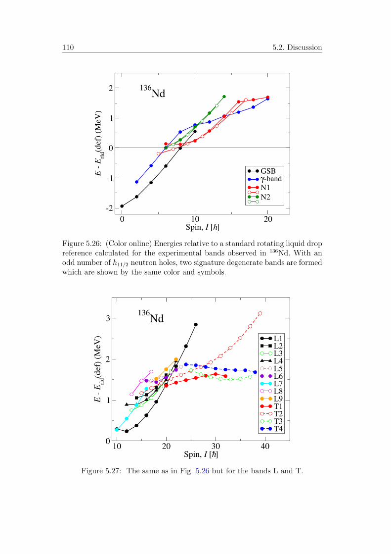
5.24 (Color online) Same as Fig. 5.23, but for D4 and D4-C. . . . . 1075.25 (Color online) Same as Fig. 5.23, but for D5 and D5-C. . . . . 1085.26 (Color online) Energies relative to a standard rotating liquid

drop reference calculated for the experimental bands observedin 136Nd. With an odd number of h

11/2 neutron holes, two sig-nature degenerate bands are formed which are shown by thesame color and symbols. . . . . . . . . . . . . . . . . . . . . . 110

5.27 The same as in Fig. 5.26 but for the bands L and T. . . . . . . 1105.28 The same as in Fig. 5.26 but for the dipole bands. . . . . . . . 1115.29 The same as in Fig. 5.26 but for the bands HD. . . . . . . . . 1125.30 (Color online) The observed low-spin bands of 136Nd are shown

relative to a rotating liquid drop reference in panel (a), with thecalculated configurations assigned to these bands given relativeto the same reference in panel (b). The panel (c) provides thedifference between calculations and experiment. . . . . . . . . 113

5.31 (Color online) The same as in Fig. 5.30 but for the medium-spinbands L. . . . . . . . . . . . . . . . . . . . . . . . . . . . . . 114

5.32 (Color online) The same as in Fig. 5.30 but for the medium-spinbands T. . . . . . . . . . . . . . . . . . . . . . . . . . . . . . 116

LIST OF FIGURES 13

5.33 (Color online) The same as in Fig. 5.30 but for the bands D. . 1185.34 (Color online) The same as in Fig. 5.30 but for the HD bands. 120

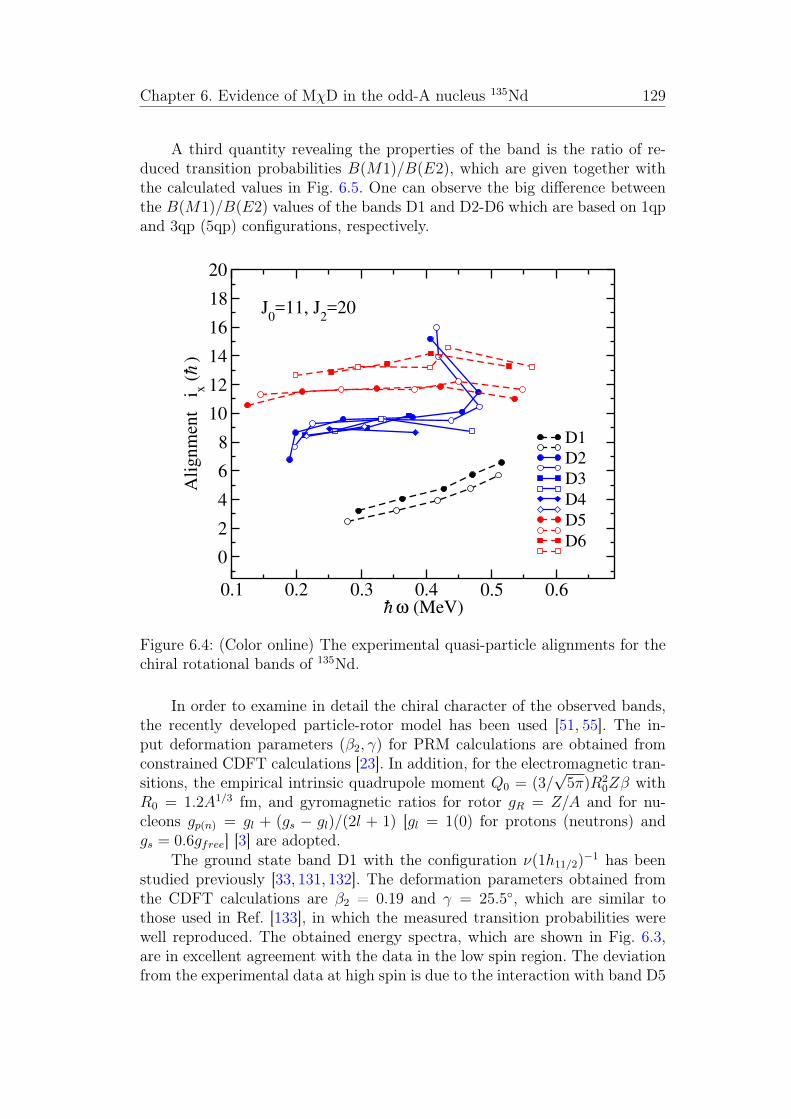
6.3 (Color online) Comparison between the experimental excitationenergies relative to a reference rotor (symbols) and the particle-rotor model calculations (lines) for the bands D1-D6. . . . . . 128

6.4 (Color online) The experimental quasi-particle alignments forthe chiral rotational bands of 135Nd. . . . . . . . . . . . . . . . 129

6.5 (Color online) Comparison between experimental ratios of tran-sitions probabilities B(M1)/B(E2) (symbols) and the particle-rotor calculations (lines) for the bands D1-D6. . . . . . . . . . 131

6.6 (Color online) The root mean square components along the in-termediate (i�, squares), short (s�, circles) and long (l�, tri-angles) axes of the rotor, valence protons, and valence neutronsangular momenta calculated as functions of spin by PRM forthe doublet bands D3 and D4 of 135Nd. . . . . . . . . . . . . 132

7.1 �-Time matrix for the clovers at the focal plane. The transitionsmarked with asterisks represent the �-decay contaminants fromthe nuclei produced in this experiment: 665 keV, 783 keV, 828keV and 872 from the �-decay of 135Ce, 761 keV and 925 keVfrom the �-decay of 137Nd. . . . . . . . . . . . . . . . . . . . . 141

7.2 Partial level scheme of 138Nd related to the isomeric state. . . 1427.3 Spectrum of prompt transitions measured by JUROGAM II

gated with selected clean transitions in 138Nd (521, 729, 884,and 973 keV) measured by the clovers placed at the focal plane. 142

7.4 Time spectra extracted from �-T matrix at the focal plane tran-sitions (521, 729, 884, and 973 keV) deexciting the 10+ isomerin 138Nd. The red line is fitted to the data. . . . . . . . . . . . 143

14 LIST OF FIGURES

List of Tables

5.1 Experimental information including the �-ray energies, energiesof the initial levels Ei, intensities I�, anisotropies RDCO andor Rac, multipolarities, and the spin-parity assignments to theobserved states in 136Nd. The transitions listed with increasingenergy are grouped in bands. The deduced values for RDCO witha stretched quadrupole gate are ⇡ 1 for stretched quadrupoleand ⇡ 0.46 for dipole transitions, while the ratio is close to 1for a dipole and 2.1 for a quadrupole transition when the gateis set on a dipole transition. The Rac values for stretched dipoleand quadrupole transitions are ⇡ 0.8 and ⇡ 1.4. . . . . . . . 84

5.2 Experimental information including the � ray energies, energiesof the initial levels Ei and the tentative spin-parity assignmentsto the observed states in 136Nd. . . . . . . . . . . . . . . . . . 97

5.3 Unpaired nucleon configurations labeled A-H and the corre-sponding parities, calculated by constrained CDFT. The ex-citation energies Ex (unit MeV) and quadrupole deformationparameters (�, �) are also presented. . . . . . . . . . . . . . . 99

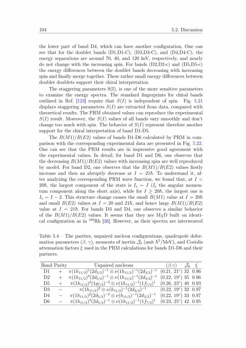
5.4 The parities, unpaired nucleon configurations, quadrupole de-formation parameters (�, �), moments of inertia J

0

(unit h2/MeV),and Coriolis attenuation factors ⇠ used in the PRM calculationsfor bands D1-D6 and their partners. . . . . . . . . . . . . . . . 104

5.5 Configuration assignments and deformation information to thebands of 136Nd. . . . . . . . . . . . . . . . . . . . . . . . . . . 119

15

16 LIST OF TABLES

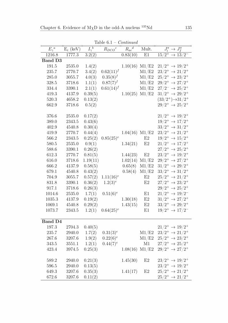
6.1 Experimental information including the �-ray energies, energiesof the initial levels Ei, intensities I�, anisotropies RDCO andor Rac, multipolarities, and the spin-parity assignments to theobserved states in 135Nd. The transitions listed with increasingenergy are grouped in bands and the transitions connecting agiven band to low-lying states are listed at the end of each bandseparated by a blank line. The deduced values for RDCO witha stretched quadrupole gate are ⇡ 1 for stretched quadrupoleand ⇡ 0.46 for dipole transitions, while the ratio is close to 1for a dipole and 2.1 for a quadrupole transition when the gateis set on a dipole transition. The Rac values for stretched dipoleand quadrupole transitions are ⇡ 0.8 and ⇡ 1.4. . . . . . . . 133

A.1 The information of JUROGAM II detector angles. . . . . . . 149

Chapter 1

Introduction

The atomic nucleus is a strongly interacting quantum many-body systemcomposed of protons and neutrons. The nuclei can contain nucleons from a fewto several hundred. This finite number of nucleons makes the nucleus become aunique system which cannot be treated in a statistical way, and its behaviour ata phase change is very different from that of ordinary matter. The finiteness ofthe nucleus is also manifest in the influence that just one nucleon may have ondetermining the nuclear properties, particularly the nuclear shape. The mainaim of the nuclear structure is to understand the distribution and motion ofthe nucleons inside the nucleus and also to study the collective motion andshape of the whole nucleus.

The work presented in this thesis is centred around two nuclei: 135Nd and136Nd, which are located in the A ⇡ 130 mass region, a fertile field of study ofthe transitional nuclei with shapes that can vary between strongly deformedin the middle of the major shell 50 < Z, N < 82 to nearly spherical closeto the shell closure [10]. A variety of shapes can also be present in a singlenucleus in different spin ranges.

At low spins, axial asymmetry was suggested for the ground states ofnuclei centered around Z = 62, N = 76 [10], in which a regular increase ofthe level energies of the observed low-lying � band, considered a sign of rigidtriaxiality has been observed, while in the surrounding nuclei the level energiespresent a staggering, which is considered a sign of soft triaxial shapes.

At medium spins, the shape can change under the polarizing effect ofunpaired nucleons resulting from broken pairs. In certain cases the triaxialshape becomes more rigid, being based on a deeper minimum of the potentialenergy surface, induced by the protons occupying low-⌦ orbitals in the lowerpart of the h

11/2 subshell, or by neutrons excited from orbitals below N =82 to low-⌦ (h

9/2, f7/2) orbitals lying above N = 82 (see, e.g., [11, 12] andreferences therein).

At high spins, the nuclei with several holes in the N = 82 shell closure,a multitude of triaxial bands have been observed in several Ce and Nd nuclei,giving strong support for the existence of stable triaxial shape up to very high

17

18 1.1. Chirality

spins. In addition, nuclei of the A ⇡ 130 mass region can also present othercoexisting shapes, e.g., axially deformed, highly deformed, and even superde-formed at high spins. This is the case for 140Nd, in which states based on aspherical shape have been observed up to spins as high as 27 h coexisting withtriaxial shapes, and in which axial superdeformed and highly deformed shapescoexist at very high spin [13,14]. In this nucleus, the bridge between the regionsof highly deformed bands present in A ⇡ 130 nuclei and the superdeformedbands present in A ⇡150 nuclei provides an insight into the development ofthe deformation between these two regions of superdeformation [14].

An additional feature of nuclei in this mass region is the presence ofisomeric states, e.g., the 10+, T

1/2 = 370 ns isomer of 138Nd, the 10+, T1/2 = 308

ns isomer of 134Ce, the 11/2�, T1/2 = 2.7 µs isomer of 137Pr, and the 6+,

T1/2 = 90 ns isomer of 136Pr [15], populated in the reaction used in the present

work, which interrupts and fragments the decay flux.The A ⇡ 130 mass region is also characterized by the existence of two

unique fingerprints of a triaxial nuclear shape: chirality and wobbling. Chiralityrepresents a novel feature of triaxial nuclei rotating around an axis which liesoutside the three principal planes of the triaxial ellipsoidal shape, which willbe discussed in detail in Section 1.1. The wobbling motion has been discussedby Bohr and Mottelson in the triaxial even-even nuclei many years ago [16].This mode represents the quantized oscillations of the principal axes of anasymmetric top relative to the space-fixed angular momentum vector or, in thebody fixed frame of reference, the oscillations of the angular momentum vectorabout the axis of the largest moment of inertia [17]. Recently, the wobblinginterpretation has been proposed for low-lying bands observed in 135Pr [17].

Thus, this region of the nuclear chart is an ideal testing ground to inves-tigate the competition between various deformations and their evolution withspins, as well as the competition between single-particle and collective modesof excitation.

1.1 ChiralityThe term chirality, was first time introduced by Lord Kelvin in 1904 in

his Baltimore Lectures [18]:"I call any geometrical figure, or group of points, chiral, and say it has

chirality, if its image in a plane mirror, ideally realized, can not be brought to

coincide with itself."

Chirality commonly exists in nature, and has important consequences infields of science as diverse as biology, chemistry, and physics. The best knownexamples of geometrically chiral objects are the human hands and the micro-scopic handedness of certain molecules. Chiral symmetry is also well knownin particle physics, where it is of a dynamic nature distinguishing between thetwo possible orientations of the intrinsic spin with respect to the momentum

Chapter 1. Introduction 19

of the particle [19].

1.1.1 Nuclear Chirality

In nuclear physics, chirality was suggested in 1997 by Frauendorf andMeng [20]. It shows up in a triaxial nucleus which rotates about an axis outof the three principal planes of the ellipsoidal nuclear shape.

Figure 1.1: Left- and right-handed chiral systems for a triaxial odd-odd nu-cleus. The symbols ~J , ~R, ~j⌫ , and ~j⇡ denote respectively the total angular mo-mentum, the angular momenta of the core, of the neutron and of the proton,respectively. Figure adopted from Ref. [1].

The simplest chiral geometry is expected in an odd-odd nucleus whenthe angular momenta of the valence proton, of the valence neutron, and ofthe core tend to be mutually perpendicular. This occurs when the collectiveangular momentum is oriented along the intermediate axis (this happens ifone assumes hydrodynamical moments of inertia), and the angular momen-tum of the high-j quasiparticle and quasihole are aligned along the short andlong axes, respectively, minimizing thus the interaction energy. These threemutually perpendicular angular momenta can be arranged into a left- or aright-handed system (see Fig. 1.1), which differ by intrinsic chirality; the twosystems are related by the chiral operator of the form � = TR(⇡), where R(⇡)corresponds to a rotation of 180�, while T is the time reversal and thereforechanges to opposite the directions of all angular momentum vectors. Chiralsymmetry in an atomic nucleus is observed because quantum tunneling occursbetween systems with opposite chirality. When chiral symmetry is thus bro-ken in the body-fixed frame, the restoration of the symmetry in the laboratoryframe is manifest as degenerate doublet �I = 1 bands with the same parity,called chiral doublet bands [21, 22]. In practice, chiral bands are near degen-erate, and show similar properties. The chiral symmetry can be identified ifsimilarities between a specific band and its partner band are observed. Thespecific fingerprints used to identify chiral doublet bands will be discussed inSection 1.2.

20 1.1. Chirality

It should be pointed out that the chirality in the nature is often static, likein the molecules, in the DNA. In the case of nucleus, the chirality is dynamic,since it is the angular momentum vector that defines a direction with respectto which the semi-axes (1, 2, 3) form a left- or right-handed system. Thenon-rotating nuclei are achiral.

1.1.2 Multiple chiral doublets (M�D)

Adiabatic and configuration-fixed constrained triaxial relativistic meanfield (RMF) approaches were developed to investigate the triaxial shape co-existence and possible chiral doublet bands in 2006 [23], which predicted anew phenomenon, the existence of multiple chiral doublets (M�D), i.e., morethan one pair of chiral doublet bands, in one single nucleus. This phenomenonwas suggested for 106Rh after examining the possible existence of triaxial de-formation and of the corresponding high-j proton-hole and neutron-particleconfigurations. Such investigation has been extended to the rhodium isotopesand the existence of M�D has been suggested in 104,106,108,110Rh [24]. The in-vestigation predicted M�D not only in 106Rh, but also in other mass regions,i.e., A ⇡ 80, and A ⇡ 130.

Recently, M�D bands have been identified in A ⇡ 130, A ⇡ 110, andA ⇡ 80 mass regions. The first experimental evidence for the existence ofM�D in the A ⇡ 130 mass region was reported in 133Ce in 2013 [25]. It wasfound that the negative-parity bands 2 and 3, and the positive-parity bands5 and 6 based on the 3-quasiparticle configurations ⇡[(1h

11/2)1(1g7/2)�1] ⌦⌫(1h

11/2)�1 and ⇡(1h11/2)2 ⌦ ⌫(1h

11/2)�1, respectively, are nearly degenerateand have similar properties. Later, Kuti et al. reported a novel type of M�Dbands in 103Rh [26], where an "excited" chiral doublet of a configuration is seentogether with the "yrast" one. This observation showed that chiral geometrycan be robust against the increase of the intrinsic excitation energy. In 78Br,two pairs of positive- and negative-parity doublet bands together with eightstrong electric dipole transitions linking the yrast positive- and negative-paritybands have been identified [27]. They were interpreted as M�D bands withoctupole correlations, being the first example of chiral geometry in octupolesoft nuclei and indicating that nuclear chirality can be robust against theoctupole correlations.

It should be noted that until now all the observed M�D bands are only inodd-odd, odd-even, and even-odd nuclei. It inspired us to search for the M�Dbands in even-even nuclei. This is one of the main aims of the experimentpresented in this thesis.


1.2 Fingerprints of the chiral bandsFrom an experimental point of view, the doublet bands must satisfy a

set of criteria in order to be recognized as chiral bands, among which themost important are the energy separation between the partners and theirelectromagnetic transitions rates.

1.2.1 Energy spectraFirstly, the appearance of near degenerate �I = 1 bands with the same

parity is considered to be one fingerprint for the chiral bands. The energiesof the partner bands should be close to each other, i.e. be nearly degenerate.What does near degenerate mean is not precisely defined since it depends onthe deformation, valence nucleon configuration and their couplings. Normally,the acceptance of a near degenerate energy is below 200 keV.

From the measured energies one can derive other observables, like theenergy staggering parameter S(I) = [E(I)�E(I�2)]/2I which can also serveas fingerprint for chiral partner bands.

Experimentally, the signature splitting between the odd- and even-spinssequences of a given dipole band is quantified by the energy staggering S(I).When the rotation axis is tilted outside the principal planes, the signature isnot a good quantum number and therefore it is more appropriate to speakabout the odd/even spin dependence of S(I). The expected typical behaviourof S(I) in a chiral band is a small odd/even staggering at low spins, whichdiminishes with increasing spin, and finally, becomes constant. Therefore, theenergy staggering parameter should be almost constant and equal for the statesof the same I, in the two chiral partners [28].

1.2.2 Electromagnetic transitions ratesThe electromagnetic transitions rates in chiral doublet bands obey im-

portant selection rules. Thus, for odd-odd nuclei, with the ⌫h11/2 ⌦ ⇡h�1

11/2

configuration coupled to a rigid triaxial rotor with � = 30�, the selectionrules for electromagnetic transitions in the chiral bands has been proposedin Ref. [29], including the odd-even staggering of intraband B(M1)/B(E2)ratios, the interband B(M1) values, as well as the vanishing of the interbandB(E2) transitions in the high spin region.

The fingerprints of the electromagnetic transitions probabilities in thechiral bands also depend on the deformation, valence nucleon configurationand their coupling. It is found that the B(M1) staggering depends stronglyon the character of the nuclear chirality, i.e., the staggering is weak in chiralvibration region and strong in the static chirality region. For partner bandsthe similar B(M1), B(E2) transitions, and the strong B(M1) staggering canbe used as a fingerprint for the static chiral rotation [30]. This result agrees

22 1.2. Fingerprints of the chiral bands

with the lifetime measurements for the doublet bands in 128Cs [31], but not in135Nd which shows a chiral vibration [32].

1.2.3 Other fingerprints

To identify chiral doublet bands besides energy spectra and electromag-netic transitions rates, as arguments in favor of chirality there are some otherspecific fingerprints. Experimentally, almost constant energy difference be-tween partners, and similar moment of inertia are always used in the discussionof the chiral doublet bands. In addition, one can examine the similarities ofthe configurations for chiral doublet bands by analysing the I-h! relation,where h! is the rotational frequency defined as h! =[E(I + 1)�E(I � 1)]/2.Generally speaking, the I-h! relation for the yrast band and its partner bandshould be similar. Furthermore, one can also examine the angular momentumgeometries of the observed doublet bands by calculating the expectation val-ues of the angular momentum components of the core, of the valence protonsand of the valence neutrons, along the intermediate, short, and long axes.

Experimentally, the chiral phenomenon has been reported in a numberof odd-odd and odd-A nuclei in the mass A ⇡ 80, A ⇡ 100, A ⇡ 130,A ⇡ 190 regions; see e.g., Refs. [21,22,25–27,31–39]. The distribution of theobserved chiral nuclei in the nuclear chart is given in Fig. 1.2.

Figure 1.2: The nuclides with chiral doublet bands (red circles) and M�D (bluepentagons) observed in the nuclear chart. The black squares represent stablenuclides. Figure adopted from Ref. [2].


1.3 Motivation of this studyThe existence of triaxially deformed nuclei has been the subject of a long

standing debate. It appears questionable how well the non-axial shape is sta-bilized. The intimate mechanism which induces such a behavior needs detailedand accurate investigations, both from the experimental and theoretical pointsof view. Recently, the wobbling and chirality, as the two unique fingerprintsof triaxiality in nuclei, have been intensively studied.

The main part of present work was undertaken with the aim of searchingfor multiple chiral bands in 136Nd, a nucleus which is the nearest even-evenneighbor of the first chiral candidate 134Pr [20] and the first reported wobbler135Pr outside of the A ⇡ 160 region [17]. In addition, an important effort wasdevoted to the detailed spectroscopy of 136Nd since most of the experimentalresults reported previously were obtained more than twenty years ago withless efficient detector arrays.

The other aim of the present work was focused on a detailed study of thechirality in 135Nd, to search for multiple chiral bands similar to those observedin the 133Ce isotone [25]. The nucleus 135Nd is one of the best known examplesof chiral vibration [32,33].

In addition to the study of the chiral bands of 135Nd and 136Nd, we devotedan important effort to searching for long-lived isomers in the populated nuclei,in particular in 135Nd and 136Nd, using the RITU+GREAT setup and therecoil tagging technique. This effort was motivated by the existence of long-lived isomers in 134Nd, 137Nd, 138Nd, 139Nd, and 140Nd [15], but not in 135Ndand 136Nd.

1.4 Outline of thesisThe remaining chapters of this thesis will be organized as follows:The relevant nuclear models needed to understand the experimental re-

sults presented in this work are described in Chapter 2.Details of the experimental techniques, and the data analysis procedures

are outlined in Chapter 3 and Chapter 4, respectively.The experimental results and discussion of 136Nd and 135Nd are reported

in Chapter 5 and Chapter 6, respectively.The search for possible long-lived isomeric states in the populated nuclei,

in particular in 136Nd and 135Nd are presented in Chapter 7.The detailed information of JUROGAM II detectors are given in Ap-

pendix A.

24 1.4. Outline of thesis

Chapter 2

Theoretical backgroud

In this chapter, some of the nuclear structure models relevant to thepresent work will be presented. The specific mechanism leading to the chi-ral mode of excitation will also be briefly discussed.

2.1 Liquid drop modelThe liquid drop model (LDM) [40] of the nucleus was historically the first

model proposed to describe the different properties of the nucleus. The ideaof considering the nucleus as a liquid drop originally came from considera-tions about its saturation properties and from the fact that nucleus has a lowcompressibility and a well defined surface [3].

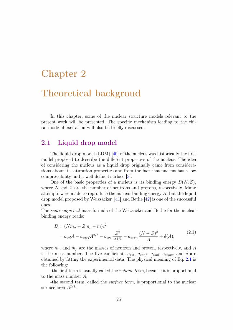
One of the basic properties of a nucleus is its binding energy B(N,Z),where N snd Z are the number of neutrons and protons, respectively. Manyattempts were made to reproduce the nuclear binding energy B, but the liquiddrop model proposed by Weizsäcker [41] and Bethe [42] is one of the successfulones.The semi-empirical mass formula of the Weizsäcker and Bethe for the nuclearbinding energy reads:

B = (Nmn + Zmp �m)c2

= avolA� asurfA2/3 � acoul

Z2

A1/3� aasym

(N � Z)2

A+ �(A),

(2.1)

where mn and mp are the masses of neutron and proton, respectively, and Ais the mass number. The five coefficients avol, asurf , acoul, aasym, and � areobtained by fitting the experimental data. The physical meaning of Eq. 2.1 isthe following:

-the first term is usually called the volume term, because it is proportionalto the mass number A;

-the second term, called the surface term, is proportional to the nuclearsurface area A2/3;

25

26 2.2. The shell model

-the third term called the Coulomb term derives from the Coulomb inter-action among protons, and is proportional to Z2;

-the fourth term called the asymmetry term reflects the fact that nuclearforce favour equal numbers of neutrons and protons, or N = Z;

-the last term called the pairing term favours configurations where twoidentical fermions are paired. It can be rewritten as follows:

�(A) =

8

<

:

apA�3/4, for even� even nuclei;

0, for even� odd nuclei;�apA

�3/4, for odd� odd nuclei.

where ap ⇡ 34 MeV [43].The LDM was very successful in predicting the nuclear binding energy

and describing how a nucleus can deform and undergo fission. As a collectivemodel, it is also particularly useful in describing the macroscopic behaviourof the nucleus. However, this is a crude model that does not explain all theproperties of the nucleus and nuclear shell structure. In particular, it fails whenit is used to explain the nuclei with magic numbers (N or Z equal 2, 8, 20, 28,50, 82, and 126). A more sophisticated model must to be developed to solvethis problem.

2.2 The shell model

As mention above, one of most important information on the shell struc-ture is the presence of magic numbers. If one of the proton or neutron numbersis equal to a magic number, then the nucleus is more stable compared withthe neighbors, has a larger total binding energy, a much larger energy of thefirst excited state, and a larger energy required to separate one nucleon.

The shell model was firstly proposed by Mayer and Jensen [44,45] in 1949to interpret the observed shell structure in nuclei. The basic assumptions ofshell model is that each nucleon moves independently in an average potentialcreated by other nucleons. The assumption made is that motion of the nucleonsis quite similar to the motion of electrons in an atom. The Schrödinger equationfor a given potential V (r), is written as

(� h2

2mr2 + V (r)) i(r) = ✏i i(r), (2.2)

where i(r) and ✏i are the eigenstates and eigenvalues representing the wavefunctions and energies, respectively. Various potential wells have been used,for example square well, infinite harmonic oscillator well, and Woods-Saxonpotential.

Chapter 2. Theoretical backgroud 27

Harmonic oscillator potentialThe harmonic oscillator potential has the form

V (r) =1

2m!2r2, (2.3)

where m is the mass of the nucleon and ! is the angular frequency of the os-cillator. The Schrödinger equation of motion for harmonic oscillator is writtenas:

(� h2

2mr2 +

1

2m!2r2) i(r) = ✏i i(r). (2.4)

The energy eigenvalues are:

✏N = h!(N +3

2), (2.5)

whereN = 2(n� 1) + l, (2.6)

with n= 1, 2, 3, ..., and l =0, 1, 2,...n�1. N is the principal quantum number,n is the radial quantum number. l is angular momentum, and it often referredto using the spectroscopic notations, s, p, d, f, g, h, ... corresponding to l =0, 1, 2, 3, 4, 5, ....

In this case, all levels with the same principal quantum number N aredegenerate, where the degeneracy is given by 2(2l + 1). The parity of eachlevel is given by ⇡ = (�1)N . This potential can only reproduce the magicnumbers 2, 8 and 20, implying that the model needs to be modified if onewants to reproduce higher magic numbers.

Woods-Saxon potentialTo improve the model, the more realistic Woods-Saxon potential [46] can

also be employed. It has the form

V (r) = � V0

1 + e(r�R)/a, (2.7)

where R = r0

A1/3 is the mean radius of the nucleus, V0

' 50 [MeV] is thedepth of the potential well, and a describes the diffuseness of the nuclearsurface, a ' 0.5 [fm].

Compared with the harmonic oscillator potential it removes the l degen-eracies of the major shells, filling the shells in order with 2(2l+1) levels, butalso in this case only the magic numbers 2, 8 and 20 are reproduced. In ad-dition, its eigenfunctions can not be solved analytically, and must be treatednumerically.

28 2.3. The deformed shell model

Spin orbit coupling

To reproduce all the magic numbers, a quite different suggestion was putforward independently by Mayer [44] and by Haxel, Jensen and Suess [45].They added a strong spin-orbit coupling term ~l · ~s into the single-particleHamiltonian.

The addition of this term splits the states with the same orbital angularmomentum l into two. The single particle total angular momentum is definedby j = l + s, and then the j values of the split-up levels are j = l ± 1

2

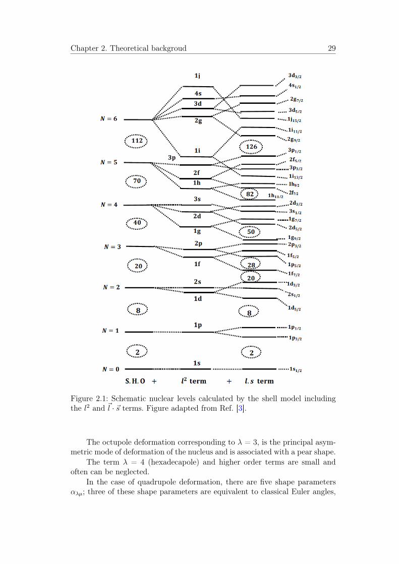
.By including the spin-orbit coupling term all magic numbers are successfullyreproduced, see Fig. 2.1. Other properties, like the spins and parities of theground states of most spherical nuclei, and the ground state magnetic momentsof nuclei are also well described. But the shell model with the spin-orbit cou-pling term is still not accurate for the description of nuclei far away from theclosed shells. These difficulties were overcome by Nilsson who introduced thedeformed shell model [47].

2.3 The deformed shell model

2.3.1 Deformed parameters

The nucleus is considered as an incompressible liquid drop with a sharpsurface or surface oscillations. In oder to investigate these oscillations, we canparametrize them in some way. The length of the radius vector R(✓,�) pointingfrom the origin to the surface can be written as

R(✓,�) = R0

[1 +1

X

�=0

�X

µ=��

↵�µY�µ(✓,�)], (2.8)

where R0

is the radius at the spherical equilibrium with the same volume, Y�µ

are the spherical harmonics. Each spherical harmonic component will havean amplitude ↵�µ, where � represents different modes of deformations. Thegeneral expansion of the nuclear surface in Eq. 2.8 allows to describe differentshapes, as displayed in Fig. 2.2.

The lowest order multipole term, � = 1, does not correspond to a defor-mation of the nucleus, but rather to a shift of the position of the center ofmass. Thus, the deformation of order � = 1 is equivalent to a translation ofthe nucleus that should be neglected for nuclear excitations.

The � = 2 multipole term corresponds to the quadrupole deformationwhich looks like ellipsoidal deformation. In this case, the nucleus shape couldbe oblate, prolate or triaxial. It turns out to be the most important mode ofexcitation of the nucleus, therefore only the � = 2 will be considered in thefollowing discussion.


Figure 2.1: Schematic nuclear levels calculated by the shell model includingthe l2 and ~l · ~s terms. Figure adapted from Ref. [3].

The octupole deformation corresponding to � = 3, is the principal asym-metric mode of deformation of the nucleus and is associated with a pear shape.

The term � = 4 (hexadecapole) and higher order terms are small andoften can be neglected.

In the case of quadrupole deformation, there are five shape parameters↵�µ; three of these shape parameters are equivalent to classical Euler angles,


Figure 2.2: The lowest four vibrations of a nucleus. The dashed lines show thespherical equilibrium shape and the solid lines show an instantaneous view ofthe vibrating surface. Figure adapted from Ref. [4].

which are related to the relative orientation of the drop in space. By a suitablerotation, we can transform to the body-fixed system characterized by threeaxes 1, 2, 3, which coincide with the principle axes of the mass distributionof the drop. Thus, the five coefficients ↵

2µ reduce to two real independentvariables ↵

20

and ↵22

= ↵2�2

(↵21

= ↵2�1

= 0), which together with the threeEuler angles, give a complete description of the system [3]. The two remainingparameters (↵

20

, ↵22

) are more convenient to be expressed in Hill-Wheeler [48]coordinates �

2

and �, as follows

↵20

= �2

cos�,

↵22

= ↵2�2

=1p2�2

sin�,(2.9)

which satisfy the condition,X

µ

|↵2µ| = ↵2

2�2

+ 2↵2

22

= �2

2

, (2.10)

where �2

is the quadrupole deformation parameter of the nucleus, while the �parameter describes the degree of triaxiality of the nuclear system, measuringthe deviation from axial symmetry.From the above definitions we can rewrite R(✓,�) as

R(✓,�) = R0

n

1 + �2

r

5

16⇡[cos�(3cos2✓ � 1) +

p3sin�sin2✓cos2�]

o

. (2.11)

The increments of the three axes in the body-fixed frame can be written interms of the �

2

and � parameters as follow

Rk �R0

R0

= �2

r

5

4⇡cos(� � 2⇡k

3), k = 1, 2, 3, (2.12)

where k = 1, 2, 3 correspond to the x, y, and z direction, respectively.


Figure 2.3: Plot of the Eq. 2.12, for k=1, 2, 3, corresponding to the increasein the axis lengths in the x, y, and z directions. Figure adopted from Ref. [5].

To easily see the evolution of the axis lengths with �, a plot of the functions�2

cos(� � 2⇡k3

) with various � and k are given in Fig. 2.3. One can see thatat � = 0� the nucleus is elongated along the z axis, while the length of x andy axes are equal (axially symmetric). With increasing �, the x axis grows atthe expense of the y and z axes, until the length of x and z axes are equal at� = 60�. This patten is repeated each 60�.

According to the Lund convention [49], the different nuclear shapes corre-sponding to the various (�

2

, �) are shown in Fig. 2.4. In this convention, for �= 0� and �120�, the nucleus is prolate, while it is oblate for � = �60� and 60�.Note that there are two different types of rotations for pure prolate and oblateshapes which can be collective- and non-collective. Collective rotation, whichoccurs when � = 0� or � = �60�, the rotational axis of nucleus is perpendicu-lar to the symmetry axis. For non-collective rotation which occurs when � =60� or � = �120�, the rotational axis of nucleus is along the symmetry axis.When � is not a multiple of 60� one has a triaxial shape. There are discretesymmetries, namely, one can interchange all three axes without changing theshape, which mean an invariance under the point group D

2

[3]. However, theinterval 0� < � < 60� is sufficient to describe all the � = 2 shapes.


Figure 2.4: Schematic of nuclear shapes with respect to the deformation param-eters (�

2

, �), as defined in the Lund convention. Figure adapted from Ref. [6].

2.3.2 The Nilsson modelThe deformed shell model was originally introduced by S. G. Nilsson [47],

which is also often referred to the Nilsson model. In this model, the anisotropicharmonic oscillator potential is used as average field, so the single-particleHamiltonian is expressed as,

H = � h2

2mr2 +

m

2(!2

xx2 + !2

yy2 + !2

zz2)� C~l · ~s�Dl2, (2.13)

where !x, !y, and !z are the oscillator frequencies, x, y, and z are the coordi-nates of a particle in the intrinsic reference system. The parameters C and Dcontrol the strength of the spin-orbit and l2 term, respectively. However, forlarge N quantum numbers, the l2-term shift is too strong and Nilsson replaced


the last term with the following form

D(l2� < l2 >N), (2.14)

where < l2 >N = 1

2

N(N + 3) is the expectation values of l2 averaged overone major shell with quantum number N. The three frequencies are chosenproportional to the inverse of the half axes ax, ay, and az of the ellipsoid:

!i = !oR

0

aii = x, y, z. (2.15)

If one only take into account the anisotropic harmonic oscillator Hamiltonian,the eigenstates are characterized by the number of oscillator quanta nx, ny,nz, and the eigenvalues are

✏0

(nx, ny, nz) = h!x(nx +1

2) + h!y(ny +

1

2) + h!z(nz +

1

2). (2.16)

In the case of axially symmetric shapes, one usually choose the z-axis as sym-metry axis and further introduce one single parameter of deformation �, so

!2

?

= !2

x = !2

y = !2(�)

✓

1 +2

3�

◆

,

!2

z = !2(�)

✓

1� 4

3�

◆

.

(2.17)

The condition of constant volume of the nucleus leads to

!x!y!z = const. = !3

0

, (2.18)

!0

is the value of !(�) for � = 0. From Eq. 2.17 and Eq. 2.18, we can get

!(�) = !0

(1� 4

3�2 � 16

27�3)�1/6, (2.19)

leading in second order to

!(�) = !0

[1 + (2

3�)2]. (2.20)

The quantity � is related to the deformation parameter �2

, as follows [47]

� ⇡ 3

2

r

5

4⇡�2

⇡ 0.95�2

. (2.21)

In the case of axial symmetry, it is more convenient to use cylindrical coordi-nates, and in this case the eigenvalues can be written as

✏0

(nz, n⇢, nl) = h!z(nz +1

2) + h!

?

(2n⇢ +ml + 1)

⇡ h!0

(N +3

2) + �(

N

3� nz),

(2.22)


withN = nz + 2n⇢ +ml = nx + ny + nz. (2.23)

Now, if one treats Eq. 2.13 by using the first order perturbation theory [43],we can obtain

E =hNnz⇤⌦|H|Nnz⇤⌦i=(N +

3

2)h!

0

+1

3�h!

0

(N � 3nz)� 2h⇤⌃

� µ0h!0

(⇤2 + 2n?

nz + 2nz + n?

� N(N + 3)

2),

(2.24)

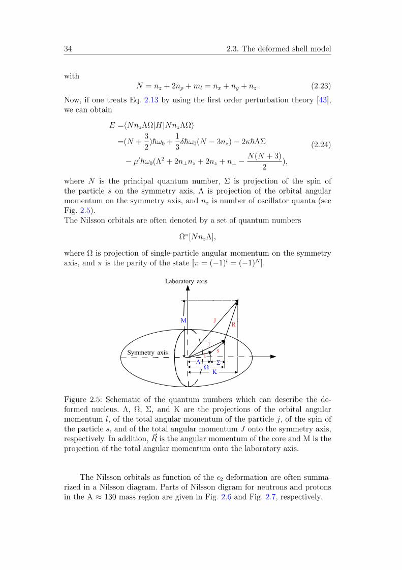
where N is the principal quantum number, ⌃ is projection of the spin ofthe particle s on the symmetry axis, ⇤ is projection of the orbital angularmomentum on the symmetry axis, and nz is number of oscillator quanta (seeFig. 2.5).The Nilsson orbitals are often denoted by a set of quantum numbers

⌦⇡[Nnz⇤],

where ⌦ is projection of single-particle angular momentum on the symmetryaxis, and ⇡ is the parity of the state [⇡ = (�1)l = (�1)N ].

Figure 2.5: Schematic of the quantum numbers which can describe the de-formed nucleus. ⇤, ⌦, ⌃, and K are the projections of the orbital angularmomentum l, of the total angular momentum of the particle j, of the spin ofthe particle s, and of the total angular momentum J onto the symmetry axis,respectively. In addition, ~R is the angular momentum of the core and M is theprojection of the total angular momentum onto the laboratory axis.

The Nilsson orbitals as function of the ✏2

deformation are often summa-rized in a Nilsson diagram. Parts of Nilsson digram for neutrons and protonsin the A ⇡ 130 mass region are given in Fig. 2.6 and Fig. 2.7, respectively.


−0.3 −0.2 −0.1 0.0 0.1 0.2 0.3 0.4 0.5 0.6

5.0

5.5

6.0

ε2

Es.

p.(h−

ω)

50

82

1g9/2

1g7/2

2d5/2

1h11/2

2d3/2

3s1/2

3/2[301]

3/2[541]

5/2[303]

5/2[532]1/2[301]

1/2[301]

1/2[550]

1/2[440]3/2[431]

3/2[431]

5/2[422]

5/2[422]

7/2[41

3]

7/2[413]

9/2[404]

1/2[431]

1/2[431]

3/2[422]

3/2[422]

5/2[413]

5/2[413]

7/2[404]

7/2[404]

7/2[633]

1/2[420]

1/2[420]

3/2[411]3/2[411]

3/2[651]

5/2[402]

5/2[642]1/2[550]

1/2[550]

1/2[301]

1/2[541]

3/2[541]

3/2[541]

3/2[301]

5/2[532]

5/2[532]

5/2[303]

7/2[523]

7/2[523]

9/2[51

4]

9/2[51

4]

11/2[505]

11/2[505]

1/2[411]

1/2[411]

1/2[660]

3/2[402]

3/2[651]

3/2[411]

1/2[400]

1/2[660]

1/2[411]

1/2[541]

1/2[301]

3/2[532] 5/2[523]

7/2[514]

9/2[505]

1/2[660]

1/2[400]

1/2[651]

3/2[651]

3/2[402]

3/2[642]

5/2[642]

5/2[402]

7/2[633]

7/2[404]

11/2[615]

13/2[606]

1/2[530]

3/2[521]

7/2[503]

1/2[770]

3/2[761]

1/2[640]

Figure 2.6: Nilsson diagram for protons in the 50 Z 80 region showingthe single-particle energies as a function of the deformation parameter ✏

2

. For✏2

>0, corresponding to the prolate shape; for ✏2

=0, corresponding to thespherical shape; for ✏

2

< 0, corresponding to the prolate shape. Labels obeythe ⌦⇡[Nnz⇤] rule.


−0.3 −0.2 −0.1 0.0 0.1 0.2 0.3 0.4 0.5 0.6

5.0

5.5

6.0

ε2

Es.

p.(h−

ω)

50

82

1g9/2

2d5/2

1g7/2

3s1/2

1h11/22d

3/2

3/2[301]

3/2[541]

5/2[532]

1/2[301]

1/2[301]

1/2[550]

1/2[440]3/2[431]

3/2[431]

5/2[422

]5/2[422]

7/2[41

3]

7/2[413]

9/2[404]

9/2[404]

1/2[431]

1/2[431]

3/2[42

2]

3/2[422]

5/2[41

3]

5/2[413]

1/2[420]

1/2[420]

3/2[411]

5/2[402]5/2

[402]

5/2[642]

7/2[404]

7/2[404]

7/2[633]

1/2[411]

1/2[411]

1/2[660]

1/2[550]1/2

[550]

1/2[301]

1/2[541]

3/2[541]

3/2[541]

3/2[301]

5/2[532]

5/2[532]

5/2[303]

7/2[52

3]

7/2[523]

9/2[51

4]

9/2[51

4]

11/2[505]

11/2[505]1/2

[400]

1/2[400]

1/2[660]

1/2[411]

3/2[402]

3/2[402]

3/2[651]

1/2[541]

1/2[301]

3/2[532]

5/2[523]

7/2[514]

1/2[530]3/2[521]

9/2[505]

1/2[660]

1/2[400]

1/2[651]

3/2[651]

3/2[402]

5/2[642]

5/2[402]

13/2[606]

1/2[770]

3/2[761]

1/2[521]

1/2[640]

Figure 2.7: Nilsson diagram for neutrons in the 50 N 80 region showingthe single-particle energies as a function of the deformation parameter ✏

2

. For✏2

>0, corresponding to the prolate shape; for ✏2

=0, corresponding to thespherical shape; for ✏

2

< 0, corresponding to the prolate shape. Labels obeythe ⌦⇡[Nnz⇤] rule.


2.4 Particle-rotor modelThe unified nuclear model and its consequences, especially for the nuclear

properties pertaining to the ground states and to the low energy region ofexcitation has been proposed by Bohr and Mottelson in 1953 [50]. It coredescribes the interplay between the motion of particles and of the collective.In this model, one considers only a few valence particles which move more orless independently in the deformed potential well of the core, and one couplethem to a collective rotor which represents the rest of the particles.

The simplest model consists of a particle in a single shell coupled to arotor. Generally speaking, one divides the Hamiltonian into two parts: anintrinsic part Hintr, which describes microscopically a valence particle, and acollective rotor part Hrot, which describes the rotations of the inert core.The total Hamiltonian is written as

H = Hintr +Hrot. (2.25)

The intrinsic part has the form

Hintr

=4

X

i=1

X

⌫

"i,⌫a†

i,⌫ai,⌫ +1

4

X

klmn

vklmna†

ka†

lanam, (2.26)

where "i,⌫ is the single-particle energy in the i-th single-j shell and v is theinteraction between the valence particles (residual interaction) which is oftenneglected.The collective rotor Hamiltonian reads:

Hrot =R2

1

2J1

+R2

2

2J2

+R2

3

2J3

, (2.27)

where the Ri are the body-fixed components of the collective angular momen-tum of the core. The total angular momentum is I = R + j, where j is theangular momentum of the valence nucleons. Thus, Hrot can be expanded intothree parts:

Hrot =3

X

i=1

I2i2Ji

+3

X

i=1

j2i2Ji

�3

X

i=1

IijiJi

, i = 1, 2, 3. (2.28)

The first term is a pure rotational operator of the rotor which acts only onthe intrinsic coordinates; the second term called recoil term, acts on the coor-dinates of the valence particle; the third term couples the degrees of freedomof the valence particles to the degrees of the freedom of the rotor.

According to the physical situation, there are two important limit cases ofthe above Hamiltonian, namely, strong coupling (deformation alignment) anddecoupling (rotation alignment).

38 2.4. Particle-rotor model

2.4.1 Strong couplingAssuming that the rotor has the 3-axis being the symmetry axis, the

moments of inertia J1

= J2

= J and K = ⌦, the corresponding rotor Hamil-tonian can be rewritten as

Hrot =1

2J⇥

(I1

� j1

)2 + (I2

� j2

)2⇤

=1

2J⇥

I2 + (j21

+ j22

� j23

)� (I+

j�

+ I�

j+

)⇤

,(2.29)

where I±

= I1

± I2

and j±

= j1

± j2

. The term (I+

j�

+ I�

j+

) correspondsto the classically Coriolis and centrifugal forces, which generates a couplingbetween the particle motion and the collective rotation. For small I, we canassume that this term is small and we just need to take into account itsdiagonal contributions, i.e., it’s treated in first order perturbation theory. Thisapproximation, in which it is assumed that the influence of the rotationalmotion in the intrinsic frame of the nucleus can be ignored, is always referredto as the adiabatic approximation or the strong coupling limit [43].

In this strong coupling case, K is a good quantum number. The angularmomentum j of the valence particle is strongly coupled to the the motion ofthe rotor (see Fig. 2.8), leading to j perpendicular to the R: this gives rise toa band I = K, I = K + 1, I = K + 2, .... . The total energy is given by

EIK = EK +1

2J⇥

I(I + 1)�K2)⇤

, K 6= 1

2, (2.30)

where EK is the quasiparticle energy.For K = 1

2

, the total energy is

EIK = EK +1

2J⇥

I(I + 1) + a(�1)I+1/2(I + 1/2)⇤

, (2.31)

where a is the decoupling factor which is calculated by

a = �X

nj

|Cnj|2(�1)j+1/2(j +1

2). (2.32)

2.4.2 The decoupling limitIn the decoupling case, the Coriolis force is strong and the coupling of the

active particle to the deformed core can be neglected. The total angular mo-mentum I is parallel to the single-particle angular momentum j (see Fig. 2.9).This gives rise to the typical �I = 2 bands. For a more detailed discussionsee Refs. [3, 43].


Figure 2.8: Schematic diagram of the strong coupling limit in the particle-rotormodel.

Figure 2.9: Schematic diagram of the decoupling limit in the particle-rotormodel.

2.4.3 Four-j shells particle-rotor model

Theoretically, various particle-rotor models have been developed to in-vestigate the exotic nuclear structure, in particular the nuclear chirality. Forexample, one-particle-one-hole PRM combined with the tilted axis cranking(TAC) approximation was first developed to study the chirality in the odd-odd nuclei [20]. Later, in order to treat more than one valence proton andone valence neutron, and also to study the nuclear chirality, the n-particle-

40 2.4. Particle-rotor model

n-hole PRM with nucleons in two single-j shells [51, 52] and three single-jshells [25,26,53,54] have been developed, respectively. In the present work, weobserved five pairs of doublet bands in 136Nd, with configurations involvingfour different single-j shells, which can not be treated by any PRM modelavailable at the time when the experimental results were obtained. Inspiredby the new obtained results in 136Nd, a n-particle-n-hole version of the PRMwith nucleons in four single-j shells was developed [55].

The total Hamiltonian of the PRM model which couples nucleons in foursingle-j shells to a triaxial rotor is similar to that of Eq. 2.25. The collectiverotor Hamiltonian Hrot is expressed as

Hrot =3

X

k=1

R2

k

2Jk

=3

X

k=1

(Ik � jk)2

2Jk

, (2.33)

where the indexes k = 1, 2, and 3 refer to the three principal axes of thebody-fixed frame, Rk, Ik, and jk denote the angular momentum of the core,of the total nucleus, and of the valence nucleon, respectively. The moments ofinertia of the irrotational flow [3] are adopted, i.e., Jk = J

0

sin2(� � 2k⇡/3).Additionally, the intrinsic Hamiltonian for valence nucleons is written as

Hintr

=4

X

i=1

X

⌫

"i,⌫a†

i,⌫ai,⌫ , (2.34)

where "i,⌫ is the single-particle energy in the i-th single-j shell given by

hsp

= ±1

2Cn

cos �⇥

j23

� j(j + 1)

3

⇤

+sin �

2p3

�

j2+

+ j2�

�

o

, (2.35)

where the plus sign refers to a particle, the minus to a hole, and the param-eter C is responsible for the level splitting in the deformed field and directlyproportional to the quadrupole deformation �

2

as in Ref. [56].The single-particle state and its time reversal state are expressed as

a†⌫ |0i =X

↵⌦

c⌫↵⌦|↵, j⌦i, (2.36)

a†⌫ |0i =X

↵⌦

(�1)j�⌦c⌫↵⌦|↵, j � ⌦i, (2.37)

where ⌦ is the projection of the single-particle angular momentum j alongthe 3-axis of the intrinsic frame and restricted to . . . , �3/2, 1/2, 5/2, . . . dueto the time-reversal degeneracy, and ↵ denotes the other quantum numbers.For a system with

P

4

i=1

Ni valence nucleons (Ni denotes the number of thenucleons in the i-th single-j shell), the intrinsic wave function is given as

|'i =4

Y

i=1

⇣

ni

Y

l=1

a†i,⌫l

⌘⇣

n0i

Y

l=1

a†i,µl

⌘

|0i, (2.38)


with ni + n0

i = Ni and 0 ni Ni.The total wave function can be expanded into the strong coupling basis

|IMi =X

K'

cK'|IMK'i, (2.39)

with

|IMK'i = 1p

2(1 + �K0

�',')

⇥|IMKi|'i+ (�1)I�K |IM �Ki|'i⇤, (2.40)

where |IMKi is the Wigner functionq

2I+1

8⇡2 DIMK , and ' is a shorthand nota-

tion for the configurations in Eq. 2.38. The basis states are symmetrized underthe point group D

2

, which leads to K� 1

2

P

4

i=1

(ni�n0

i) being an even integer.Once obtained the wave functions of the PRM, the reduced transition

probabilities B(M1) and B(E2) can be calculated with the M1 and E2 oper-ators [57].

Note that due to the inclusion of n-particle-n-hole configurations withfour single-j shells, the size of the basis space is quite large. It is rather time-consuming in the diagonalization of the PRM Hamiltonian matrix. In orderto solve this problem, a properly truncated basis space by introducing a cutofffor the configuration energy

P

i,⌫ "i,⌫ was adapted which is similar in the shell-model-like approach (SLAP) [58,59]. In this way, the dimension of the PRMmatrix is reduced to ⇠ 5000-10000, , while maintaining the energy uncertaintywithin 0.1% [55].

This new version of the PRM has been applied to investigate the energyspectra, the electromagnetic transition probabilities, as well as the angularmomentum geometries of the five pairs of nearly degenerate doublet bands in136Nd, which are discussed in detail in Section. 5.2.2.

2.5 Cranked Nilsson-Strutinsky modelOne of the most important and widely used models in the high-spin study

is the cranked Nilsson-Strustinsky (CNS) model [60–63], which successfullydescribes the high-spin states of nuclei. In the present work, this model wasapplied to discuss the various band structures in 136Nd (see Section. 5.2.3). Inthe Nilsson-Strustinsky method, the total energy of the nucleus is split intoan average part, parametrized by a macrosopic expression, and a fluctuatingpart extracted from the variation of the level density around the Femi surface.The microscopic part using the Strustinsky shell correction [63].

2.5.1 Cranking modelTo get a deeper insight into the properties of rotating nuclei from a micro-

scopic point of view, the cranking model was intruduced by Inglis [64,65]. The

42 2.5. Cranked Nilsson-Strutinsky model

basic idea of the cranking model is the following classical assumption: if oneintroduces a coordinate system which rotates with constant angular velocity !around x-axis, the motion of the nucleon in the rotating frame is rather simplewhen the angular frequency is properly chosen; in particular, the nucleons canbe thought of as independent particles moving in an average potential wellwhich is rotating with the coordinate frame [3].The single-particle Hamiltonian in the rotating system h! is given as,

h! = h� !jx, (2.41)

where h is the single-particle Hamiltonian in the laboratory system and jx isthe x-component of the single-particle angular momentum.Thus, the total energy in the laboratory system is calculated as,

Etot =X

i

< �!i |h|�!

i >=X

i

e!i +X

i

! < �!i |jx|�!

i >, (2.42)

and the total spin I is

I ⇡ Ix =X

i

< �!i |jx|�!

i >, I � 1, (2.43)

where �!i are the single-particle eigenfunction in the rotating system and

e!i =< �!i |hw|�!

i > the corresponding eigenvalues, also called single-particleRouthians. The slope of the Routhian corresponds to the alignments ix. It iswritten as

ix = �de!id!

. (2.44)

Note that the Eq. 2.41 Hamiltonian is dependent on the rotational fre-quency !, and therefore it breaks the time-reversal symmetry, but remainsinvariant with respect to space inversion (parity invariance), which means thatthe parity (⇡) is a good quantum number. In addition, the cranking Hamil-tonian is invariant with respect to rotation through an angle ⇡ around therotating axis [60].

Rx(⇡) = e�i⇡jx , (2.45)

with eigenvaluer = e�i⇡↵, (2.46)

where ↵ is the signature quantum number. The single-particle orbitals can beclassified with respect to the signature quantum number ↵, which can takevalues ↵i = +1

2

(ri = �i) or ↵i = �1

2

(ri = i). In addition, the signature ↵relates to the total angular momentum.For a system with an even number of nucleons,

↵ = 0 (r = +1), I = 0, 2, 4... ,

↵ = 1 (r = �1), I = 1, 3, 5... .(2.47)


For a system with an odd number of nucleons,

↵ = +1

2(r = �i), I =

1

2,5

2,9

2... ,

↵ = �1

2(r = +i), I =

3

2,7

2,11

2... .

(2.48)

As mentioned above, the parity ⇡ is a good quantum number, which togetherwith the signature ↵ can be used to describe the Routhians of the quasiparti-cles.

The advantage of using the cranking model is that it gives a microscopicdescription of rotating nuclei, in which the total angular momentum is thesum of single-particle angular momenta, and thus collective and non-collectiverotations can be treated on the same footing. However, this model is a semi-classical approximation due to the fact that the rotation is imposed externally.A fixed rotation axis is used in the model which also breaks the rotational in-variance. In addition, another important shortcoming of the cranking modelis that the wave functions are not eigenstates of the angular momentum oper-ator, which causes difficulties, i.e., a proper calculation of the electromagnetictransition probabilities [43,60].

The rotating harmonic oscillator

Many features of the high-spin structure of nuclei can be easily illustratedwith the rotating (cranked) harmonic oscillator potential because of its sim-plicity, and allowing to express in analytic form all matrix elements.

If only the orbital angular momentum is considered, the cranking Hamil-tonian reads

h! = hosc � !l1

, (2.49)

wherehosc = � h2

2m4+

m

2(!2

1

x2

1

+ !2

2

x2

2

+ !2

3

x2

3

), (2.50)

andl1

= x2

p3

� x3

p2

. (2.51)

The oscillator frequencies !1

, !2

and !3

are expressed in the standard waythrough the deformation coordinates ✏

2

and � [66]:

!i = !0

(✏2

, �)[1� 2

3✏2

cos(� + i2⇡k

3)] i = 1, 2, 3. (2.52)

Introducing boson creation and annihilation operators, a+i and ai, see Ref. [60],the cranking Hamiltonian Eq. 2.49 can be written in the form

hw =3

X

i=1

h!i(a+

i ai +1

2)� !l

1

, (2.53)


where

l1

=!2

+ !3

2(!2

!3

)1/2(a+

2

a3

+ a+3

a2

)� !2

� !3

2(!1

!3

)1/2(a+

2

a+3

+ a2

a2

). (2.54)

Now, we can get the single-particle eigenvalues of h! [43]

e!v = h!1

(n1

+1

2) + h!↵(n↵ +

1

2) + h!�(n� +

1

2), (2.55)

where n1

, n↵ and n� specify the number of quanta in the three normal-modedegrees of freedom (directions).

A further quantity of interest is the expectation value of l1

. The diagonalparts of this operator are easily obtained and thus, for an orbital that ischaracterized by the occupation numbers n

1

, n↵ and n�:

< l1

> ⇡ (p

1 + p2)1/2(n� � n↵). (2.56)

The total quantities of the A-particle system will now be considered withthe A-particles generally filling the lowest or close-to-lowest energy orbitals ofthe cranked harmonic oscillator. For this purpose, we define the quantities

⌃k =X

⌫ occ

< ⌫|a+k ak +1

2|⌫ >=

X

⌫ occ

(nk +1

2)⌫ . (2.57)

The index k takes the values k = 1, ↵, and � (or k = 1, 2 and 3 for ! = 0)and the summation extends over the occupied orbitals, |⌫ >. Then the specificconfiguration in the rotating frame is defined by (⌃

1

,⌃↵,⌃�).The total energy in the rotating system is given by

E =X

⌫ occ

h⌫|hw|⌫i = h!1

⌃1

+ h!↵⌃↵ + h!�⌃�. (2.58)

The total energy in the laboratory system is calculated as the sum of expec-tation values of the Hamiltonian hosc

E =X

⌫ occ

h⌫|hosc|⌫i =X

⌫ occ

h⌫|h! + !l1

|⌫i = E! + !I. (2.59)

In addition, for a fixed configuration (⌃1

,⌃↵,⌃�) and spin I, the mini-mized energy E can be obtained.

The cranked single-particle Nillsson Hamiltonian

The cranked single-particle Nilsson Hamiltonian h! is given by [61]

h! = hh.o.(✏2, �) + 2h!0

⇢2✏4

V4

(�) + V 0 � !jx, (2.60)


where hh.o.(✏2, �) is the anisotropic harmonic oscillator Hamiltonian, ⇢ is theradius in the stretched coordinate system.The hexadecapole deformation potential V

4

(�) is defined to obtain a smoothvariation in the �-plane, so it does not break the axial symmetry when � =�120�,�60�, 0�, and 60�. It has the form

V4

(�) = a40

Y40

+ a42

(Y42

+ Y4�2

) + a44

(Y44

+ Y4�4

), (2.61)

where the parameters a4i are chosen as

a40

=1

6(5cos2� + 1), a

42

= � 1

12

p30sin2�, a

44

=1

12

p70sin2�. (2.62)

The term V 0 is the Nilsson potential which as defined in Ref. [47].The diagonalization of the Hamiltonian of Eq. 2.60 gives the eigenvalues

e!i and eigenfunctions of the eigenvectors �!i . Furthermore, the single-particle

energies in the laboratory system and the single-particle angular momentumalignments in the rotating system can be obtained.

Note that the sum over the occupied single-particle states from phe-nomenological potentials, such as the Nilsson or Woods-Saxon potentials,turned out to yield poor approximations to average nuclear properties andtheir deformation dependence [3]. To overcome these problems, the total en-ergies are renormalized to a rotating liquid drop behaviour.

2.5.2 The rotating liquid drop model

The energy of a rotating nuclear liquid drop at the fixed spin I0

has theform

ERLD(I0) = ELD(I = 0) +1

2Jrig(✏)I20

, (2.63)

where Jrig(✏) is the rigid body moment of inertia and ✏ =(✏2

, �, ✏4

...). The totalenergy in the liquid-drop model is given by [60]

ERLD(I0) =� av⇥

1� kv(N � Z

A)2⇤

A+3

5

e2Z2

Rc

[Bc(✏)� 5⇡2

6

� d

Rc

)2]

+ as[1� ks(N � Z

A)2]A2/3Bs(✏),

(2.64)

where Bc(✏) and Bs(✏) are the coulomb and surface energies of a nucleus witha sharp surface in units of their corresponding values at a spherical shape [60],respectively. The second term in the Coulomb energy is a (shape-independent)diffuseness correction with d being the diffuseness. In addition, we often definethe Coulomb energy constant ac as ac =

3

5

e2

Rc

.


2.5.3 The configuration-dependent CNS approachFollowing the standard Nilsson-Strutinsky method [61, 67], the total nu-

clear energy Etot at a specific deformation ✏ and a specific spin I0

is obtainedas a sum of the rotating liquid drop energy and the shell correction energy

Etot(✏, I0) = ELD(✏, I = 0) +1

2Jrig(✏)I20

+ Esh(✏, I0). (2.65)

The shell correction energy is defined as the difference between the discreteand smoothed single-particle energy sums,

Esh(I0) =X

ei(!, ✏)�

�

�

I=I0�X

eei(e!, ✏)�

�

�

eI=I0, (2.66)

where the smoothed sum (indicated by ⇠) is calculated using the Strutinskyprocedure [43,67]. In the numerical calculations, it is parametrized as

X

eei(e!, ✏)�

�

�

eI=I0=X

eei(e!, ✏)�

�

�

eI=0

+1

2Jstr(✏)I20

+ bI40

, (2.67)

where Jstr is the (Strutinsky) smoothed moment of inertia and E0

is the valueofP

eei(e!, ✏)|eI=I0for eI = 0. The E

0

, I20

, and bI40

terms were introduced inRef. [49]. The constants Jstr, E

0

, and b are determined by calculating thesmoothed sum at the different frequencies (see Ref. [49]). Using these formu-las, we can calculate the total nuclear energy as a function of spin I at anydeformation.

Furthermore, in oder to get a better physical understanding of the re-lation between the level density and the shell energy, it is useful to rewritethese equations slightly and make some approximations. A quasi-shell energyis defined as

Equasi�sh(!, ✏) =X

ei(!, ✏)�X

eei(!, ✏). (2.68)

This definition is important because it shows that the numerical values of Esh

and Equasi�sh are very similar. The Esh is defined exactly analogous to thestatic shell energy. Thus, ! enters very much as a deformation and we cantake over all our experience from the static case.

In order to obtain the renormalized frequency, the formulas above arecombined by rewriting the total energy as

Etot(I0) =X

ei(!, ✏)�

�

�

I=I0+ ELD(✏, I = 0)� E

0

+n 1

2Jrig

� 1

2Jstr

o

I20

� bI40

.

(2.69)With the frequency given by @E/@I, the resulting renormalized frequency is

!ren(I0) = ! +⇣ 1

2Jrig

� 1

2Jstr

⌘

I0

+ bI40

, (2.70)


where b value is always very small, thus we can neglect the bI40

term. Fur-thermore, for highly deformed bands with no pairing I = Jstr!, using thisapproximation, we can obtain

!ren = (Jstr/Jrig)!. (2.71)

With this renormalization being in the range 1.2-1.3, depending on the defor-mation, frequencies in Routhian diagrams are directly comparable with exper-imentally observed frequencies only if the Routhians are plotted as a functionof !ren.

Note that in the present used version of the cranked Nilsson-Strutinskymodel the pairing correlations have been neglected. The neglect of pairing hasan advantage in that the tracing of a fixed configuration undergoing drasticdeformation changes becomes possible over the considerable spin range of aband up to termination. Furthermore, in the present study, we are mainlyinterested in the very high spin states of nuclei, for which the deformationchanges play an more important role than the pairing.

2.6 Tilted axis cranking covariant density func-tional theory

Magnetic rotation is an exotic rotational phenomenon observed in weaklydeformed or near-spherical nuclei which are interpreted in terms of the shearsmechanism [68]. Since their first observation, the magnetic bands have beenmainly investigated in the framework of tilted axis cranking (TAC) [20,69,70].In the last decades, the covariant density functional theory (CDFT) and itsextensions have been proved to be successful in describing a series of nuclearproperties, like ground-states and excited states, radii, single-particle spec-tra, magnetic rotation, and collective motions, etc. Recently, the tilted axiscranking covariant density functional theory (TAC-CDFT) [71–75] has beendeveloped and applied for the description of the chiral bands.

2.6.1 Tilted axis crankingIn the standard cranking model, it is assumed that the rotational axis

coincides with one of the principal axes of the deformed density distribu-tion. Such principal axis cranking (PAC) solutions always exist. In the TACapproach, the rotational axis does not coincide with any principal axis. Atdifference from the PAC model, the signature is not a good quantum number.The TAC model is based on the mean field theory that permits the calculationof the orientation of the deformed field in space together with the parametersthat define its shape. Thus, one may easily study multi-quasiparticle excita-tions, and the consequences of changes of the deformation or the pairing. It

48 2.6. Tilted axis cranking covariant density functional theory

gives transparent classical vector diagram pictures of the angular momentumcoupling, which is of great help to understand the structure of rotation bands.The drawback of the TAC model is that it cannot describe the gradual onset ofsignature splitting as well as the mixing of bands with substantially differentquasiparticle angular momentum as in the standard cranking theory [71].

Assuming that the rotational axis is the z-axis and with a constant angularvelocity !, the corresponding Hamiltonian in intrinsic frame is given as

H0= H � !Jz. (2.72)

In Ref. [70], the H term is defined as a sum of the spherical Hamiltonian andthe pairing plus quadrupole interaction,

H = Hsph � �

2

2

X

µ=�2

Q+

µQµ �GP+P � �N, (2.73)

with the spherical partHsph =

X

k

✏kc+

k ck, (2.74)

where Hsph is parameterized in the same way as the Nilsson Hamiltonian, thepairing interaction is defined by the monopole pair field P+, the quadrupoleinteraction is defined by the operators Qµ, and � is the chemical potential.As written above all expressions are only accounting for one kind of particles.Thus, they are understood as sums of a proton and a neutron part, and theterms �GP+P and ��N for both protons and neutrons. In practice, theactual values of the force constants � and G depend on the configuration spaceunder consideration and are determined from experimental data. A detaileddescription of the TAC model can be found in the Refs. [3,7,69,70]. As in thepresent work we are interested in the chiral motion, in the following we willexamine the TAC solutions for specific rotation axes.

Rotation about a principal axis

If the axis of rotation (z) coincides with one of the principal axes, theorientation angles defined as in the case of spherical coordinates, are satisfyingthe condition:

✓ = 0,⇡

2; � = 0,

⇡

2. (2.75)

The upper panel of Fig. 2.10 shows this case, in which J has the direction ofone of the principal axes and Rz(⇡) satisfies the relation

Rz(⇡)|i = e�i↵⇡|i, (2.76)

which means that the signature quantum number ↵ takes the values I = ↵+2n,n = ±1, ±2..., giving rise to a band characterized by �I = 2 transitions.


Figure 2.10: Discrete symmetries of the mean field of a rotating triaxial re-flection symmetric nucleus. The axis of rotation (z) is marked by the circulararrow. The rotational band structures associated with each symmetry type arepresented on the right side. This figure was taken from Ref. [7].

Rotation around an axis in a principal plane

If the axis of rotation (z) does not coincide with any of the principal axes,but still lies in one of the three principal planes, we call such solution planar.The orientation angles satisfy the relations:

✓ 6= 0,⇡

2; � = 0,

⇡

2,

or

✓ = 0,⇡

2; � 6= 0,

⇡

2.

(2.77)

The middle panel of Fig. 2.10 displays this case, in which the axis of rotationlies in one of the three principal planes 1-2, 2-3 or 1-3 and the Rz(⇡) symmetryis broken, that is it satisfies the relation

Rz(⇡)|i 6= e�i↵⇡|i, (2.78)

50 2.6. Tilted axis cranking covariant density functional theory

which means the signature is not a good quantum number anymore and thusthere is no restriction on the angular momentum I, giving rise to a bandcharacterized by �I = 1 transitions..

Rotation around an axis out of a principal plane

If the axis of rotation (z) is out of the three principal planes, we call sucha solution aplanar, and the orientation angles satisfy the relations

✓ 6= 0,⇡

2; � 6= 0,

⇡

2. (2.79)

The lower panel of Fig. 2.10 displays the aplanar case in which the rotationalaxis does not lie in one of the principal planes. In this case, TRy(⇡) symmetryis broken. The TRy(⇡) is the time-reversal operator combined with rotationabout the y-axis by ⇡. The two combinations have opposite chirality, cor-responding the left- and right-handed frames. The breaking of the TRy(⇡)symmetry causes two degenerate doublet �I = 1 bands with the same parity.

2.6.2 TAC-CDFTThe covariant density functional theory (CDFT) can be traced back to

the successful relativistic mean-field (RMF) models introduced by Walecka andSerot [76,77], which was further developed by many physicists. In the following,we will give a brief description of the tilted axis cranking covariant densityfunctional theory (TAC-CDFT) based on the point-coupling interaction [75].

The starting point of the CDFT is an effective Lagrangian density of theform

L = Lfree + L4f + Lhot + Lder + Lem, (2.80)which is divided into five terms. The Langrangian density for free nucleonsLfree,

Lfree = (i�µ@ �m) , (2.81)the four fermion point-coupling terms L4f ,

L4f =� 1

2↵S( )( )� 1

2↵V ( �µ )( �µ )

� 1

2↵TS( ~⌧ )( )� 1

2↵TV ( ~⌧�µ )( ~⌧�

µ ),(2.82)

the higher order terms Lhot accounting for the medium effects,

Lhot =� 1

3�S( )

3 � 1

4�S( )

4 � 1

4�V [( �µ )( �

µ )]2, (2.83)

the derivative terms Lder to simulate the effects of finite-range,

Lder =� 1

2�S@⌫( )@

⌫( )� 1

2�V @⌫( �µ )@

⌫( �µ )

� 1

2�TS@⌫( ~⌧ )@

⌫( )� 1

2�TV @⌫( ~⌧�µ ),

(2.84)


and the electromagnetic interaction term Lem,

Lem =� 1

4F µ⌫Fµ⌫ � e

1� ⌧3

2 �µ Aµ, (2.85)

where m is the nucleon mass and e is the charge unit for protons. Aµ and Fµ⌫

are the four-vector potential and field strength tensor of the electromagneticfield, respectively. There are in total 11 coupling constants, ↵S, ↵V , ↵TS, ↵TV ,�S, �S, �V ,�S, �V , �TS, and ↵TV , in which ↵ refers to the four-fermion term, �and � respectively to the third- and fourth-order terms, and � the derivativecouplings. The subscripts S, V , and T respectively indicate the symmetries ofthe couplings, i.e., S stands for scalar, V for vector, and T for isovector [78].

The Hamiltonian density, i.e., the 00 components of the energy-momentumtensor, can be obtained by the Legendre transformation

H = T 00 � @L@�i

�i � L, (2.86)

where �i is the nucleon or photon field. Thus, the total Hamiltonian is givenas

H =

Z

d3xH. (2.87)

In TAC-CDFT, it’s assumed that the nucleus rotates around an axis in thexz plane, the Lagrangian in Eq. 2.80 is transformed into a frame rotatinguniformly with a constant rotational frequency,

⌦ = (⌦x, 0,⌦z) = (⌦cos✓⌦

, 0,⌦sin✓⌦

), (2.88)

where ✓⌦

is the tilted angle between the cranking axis and the x-axis. TheDirac equation with nucleon potentials has the form

[↵ · (�ir� V ) + �(m+ S(r)) + V (r)� ⌦ · J ] k = ✏k k, (2.89)

where J is the total angular momentum of the nucleon spinors, ✏k representsthe single-particle Routhains for nucleons, and the relativistic fields S(r) andV µ(r) are connected in a self-consistent way to the nucleon densities and cur-rent distributions, which are obtained from the single-nucleon spinors k.

The iterative solution of these equations yields single-particle energies,expectation values for the three components hJii of the angular momentum,total energies, quadrupole moments, transition probabilities, etc. The magni-tude of the angular velocity ! is connected to the angular momentum quantumnumber I by the semiclassical relation hJi2 = I(I + 1), and its orientation isdetermined by minimizing the total Routhian self-consistently. The detailedformalism of TAC-CDFT can be seen in Refs. [71–75,78].

In the present work, the TAC-CDFT calculations have been applied forthe doublet bands built on the 4- and 6-quasiparticle configurations identifiedin 136Nd, which will be presented in Section. 5.2.1.

52 2.7. Transition probabilities

2.7 Transition probabilitiesThe ratios of reduced transition probabilities (B(M1)/B(E2)) are cru-

cial in the intrinsic nuclear structure studies. B(M1)/B(E2) ratios can beextracted from the experimental transition energies and intensities, togetherwith the multipole mixing ratio (angular distributions/correlations). It’s alsopossible to obtain them from the measurement of the lifetime of nuclear states.Ratios of reduced transition probabilities can be extracted as

B(M1; I ! I � 1)

B(E2; I ! I � 2)=

0.697E5

�(M1; I ! I � 1)

E3

�(E2; I ! I � 2)

I�(M1)

I�(E2)

1

1 + �2

(2.90)

where I�(M1)/I�(E2) is ratio of the the intensities of the � rays, � denotesthe mixing ratio ration of the �I = 1 transitions. The B(M1)/B(E2) ratiosare expressed in units of (µN/eb)2 and E� in MeV.

Theoretically, the B(M1)/B(E2) ratios can be calculated using the semi-classic formalism of Dönau and Frauendorf [79, 80].

Chapter 3

Experimental techniques

One of the goals of the nuclear structure physics is to understand theproperties of the high-spin states. Investigations on the nuclear structure athigh spins require specific experimental techniques. The population of high-spin states in nuclei, the methods of measurements, and the experimentalfacilities used in this work are presented in this chapter.

3.1 Heavy-ion fusion-evaporation reactionsThere are many types of reactions to produce excited nuclei, i.e., inelas-

tic scattering, Coulomb excitation, heavy-ion fusion-evaporation reaction (aheavy-ion is defined as a nucleus with mass number A > 4). Among them, thefusion-evaporation is one of the most useful in the high-spin physics since itcan produce excited nuclei in very high-spin states. To overcome the Coulombbarrier Vc form a compound nucleus, the minimum beam energy required is

Vc = 1.44Zb · Zt

Rb +Rt

[MeV], (3.1)

where the subscripts b and t denote projectile and target, respectively. Rb,t =

r0

A1/3b,t is the radius of respective nucleus and Zb,t represent the atomic num-

bers. After fusion of the projectile and target, the compound nucleus is in ahighly excited state, with the excitation energy of

Eex = Q+ Ecm, (3.2)

where Ecm is the kinetic energy of the system in the center of the mass frameand the Q-value is the reaction energy. They are given by

Q = (Mb +Mt �Mcn), Ecm =mt

mb +mt

Elab.. (3.3)

We can also estimate the maximum angular momentum transferred in a fusionevaporation reaction, lmax, which can be expressed as

53

54 3.1. Heavy-ion fusion-evaporation reactions

n

n

Targetnucleus

compound nucleus

Fast fission

I x

Ix

γ-ray emission

BeamNucleus

Fusion

Ground state

n

p

Particle evaporation

Figure 3.1: Schematic illustration the heavy-ion fusion-evaporation reactionforming a compound nucleus and its decay.

l2max =2µR2

h2

(Ecm � Vc), (3.4)

where µ = Rb

Rt

Rb

+Rt

is the reduced mass of the compound nuclear system.In fusion-evaporation reactions, a compound nucleus with very high ex-

citation energy and angular momentum is formed when a heavy-ion beambombards a target nucleus. If the compound nucleus does not fission, thenthe compound hot system will cool down by evaporation of particles, such asneutrons, protons, and ↵ particles. Each of the emitted particles carries awayan energy of ⇡ 8 MeV and 1�2 h of angular momentum. Finally, the residualnucleus produced after the evaporation of the particles loses the rest of exci-tation energy and almost all angular momentum via �-ray emission, until itreaches the ground state. The dominant part of deexcitations of the residualnucleus proceeds by �-ray emission. Therefore, the �-ray spectroscopy as anefficient method was used to the study of excited states of nuclei. Generally,in the �-ray spectroscopy one uses energy-sensitive HPGe detectors for themeasurement of the � rays emitted from a residual nucleus, and one analizesthe properties of � rays, such as the energy, the multipolarity from angulardistribution or angular correlation, the electromagnetic character from polar-ization. A schematic picture showing the formation and decay of the compoundnucleus is given in Fig. 3.1.

Chapter 3. Experimental techniques 55

3.2 Interaction mechanisms of the �-rays withmatter

In order to understand how to extract the information carried by the �-rays, a knowledge of the �-ray interactions with matter is important. Onlythree major types of interaction play a significant role in nuclear spectroscopymeasurements: photoelectric absorption, Compton scattering, and pair produc-

tion. These processes are schematically shown in Fig. 3.2.

3.2.1 Photoelectric absorptionPhotoelectric absorption is an interaction in which the incident �-ray

photon disappears, namely, is fully absorbed. In this case, a photoelectron isemitted from one of the electron shells (Eb) of the absorber atom with a kineticenergy given by the incident photon energy E� minus the binding energy ofthe electron in its original shell, Ee = E��Eb. The process is shown in Fig. 3.2(a). After the electron has been emitted, a hole is created in the shell, X-raysare emitted in the process of filling the created hole, but it is also possiblethat the another electron, called Auger electron, is emitted. For typical �-rayenergies, the photoelectric effect is most likely to occur in the K shell, whichhas typical binding energies ranging from a few keV for low-Z materials totens of keV for the materials with high-Z.

Figure 3.2: (a) Photoelectric absorption, (b) Compton scattering, (c) Pairproduction.

3.2.2 Compton scatteringIn this process, the incident �-ray with energy E� is scattered by an elec-

tron, creating a recoil electron and a scattered �-ray photon deflected throughan angle ✓ with respect to its original direction, with the energies of Ee andE

0�, respectively. This process is illustrated in Fig. 3.2 (b).

56 3.3. High-purity Germanium �-ray detector

The energy of the scattered photon is given by

E0

� =E�

1 + ( E�

m0c2)(1� cos✓)

, (3.5)

where moc2 = 0.511 MeV is the rest mass energy of the electron. The kinetic

energy of the recoil electron is

Ee = E� � E0

� = E�

"

1� 1

1 + ( E�

m0c2)(1� cos✓)

#

. (3.6)

From the above equations, two extreme cases can be identified:1. When the scattering angle ✓ = 180�, the incident �-ray is backscat-

tered towards its original direction, while the electron recoils along the inci-dence direction, the recoil electron having the maximum energy. This is theso-called "Compton edge" in a �-ray spectrum, which corresponds to an energy

Ee|✓=180

� = E�

2 E�

m0c2

1 + 2 E�

m0c2

!

. (3.7)

2. When the scattering angle ✓ = 0�, Ee ⇡ 0.

For most �-ray spectroscopy experiments, Compton scattering is the maincause of false events and decrease the P/T ratio of the spectra. To overcomethese drawbacks anti-Compton shields were developed, which will be discussedin the section 3.3.

3.2.3 Pair productionThe third effect shown in Fig. 3.2 (c) is pair production. The process

occurs when an incident �-ray within the strong electric field near the atomicnucleus, and results in the creation of an electron-positron pair. Since an energyof 2m

0

c2 is required to create the pair, a minimum � energy of 1.02 MeV isrequired to make the process energetically possible. After their production,both the electron and positron travel through the detector medium loosingtheir energy. Once kinetic energy of the positron becomes very low, it willannihilate or combine with a electron in the absorbing medium and emissionof two anti-parallel 0.511 MeV �-rays. This process is shown in Fig. 3.2 (c).

3.3 High-purity Germanium �-ray detectorIn the 1960s, the Ge(Li) detectors were developed which marked the birth

of high resolution �-ray spectroscopy. In the 1980s, the more advanced HPGe


detectors became available widespread. The HPGe detector has many advan-tages over the Ge(Li) detector, i.e., HPGe offer the best compromise betweenenergy resolution and efficiency; it also can be stored at room temperaturewhich reduces storage costs and facilitates easier transportation, while Ge(Li)detectors must be continuously maintained at low temperature [81]. In addi-tion, a detector system based on HPGe has good energy resolution, good P/Tratio, high efficiency and rather good timing properties which allow to extractthe events of interest from complex � spectra. In the 1990s, nuclear physicistsbuilt the next generation of �-ray arrays, i.e., GAMMASPHERE and EU-ROBALL, with the aim to realize an ultimate 4⇡ array of escape-suppressedGe detectors. More recently the first phase of Advanced GAmma Tracking Ar-ray (AGATA) was complete, as a new generation �-ray spectrometer. AGATAis based on the technique of �-ray energy tracking in electrically segmentedhigh-purity germanium crystals [82].

Figure 3.3: Reverse bias of the p-n junction.

A HPGe detector is generally operated as fully depleted detector. Reverse-biasing requires that a positive voltage be applied to the p-n junction, asshown in Fig. 3.3. At the p-n junction, the "built-in" electric field and theapplied electric field are in the same direction. A thicker depletion region iscreated when these two fields add. The depletion region is a region of netzero charge, without free electrons and holes. The �-ray interact with thegermanium crystal within the depleted zone, producing electron-hole pairswhich move towards the detector outer contacts. The produced charge inducesa voltage pulse signal in a preamplifier. There are two major types of HPGedetectors: planar and coaxial. The planar detector usually used to measurethe complex low-energy �-ray in the range of 10 keV to a few hundred keV orX-rays. It achieves the best energy resolution due to low capacitance. Coaxialdetectors have a large detection efficiency at high �-ray energies, and are usedto measure � in the range of 10 keV to 10 MeV.

58 3.4. The JUROGAM II array

Compton suppression with BGO detectorsThe dominating contribution to the background in �-ray spectroscopy is

come from the incomplete energy deposition of the incoming photon in the de-tector volume due to the Compton scattering. The Compton scattered �-rayswill result a continuous background in the �-ray spectrum which consequentlyraises the detection limit for low energies and also decrease P/T ratio. In orderto counteract these unwanted effects, we can suppress the Compton scattered�-rays by surrounding the HPGe detector with a secondary veto detector,which usually is a scintillator. The majority of the �-rays that are scatteredout of the HPGe detector are then detected in the surrounding scintillator.Producing a veto signal that is used to eliminate the partially absorbed eventsfrom the spectra of the Ge detector. Generally speaking, the secondary detec-tor is expected to have a high detection efficiency and high density to absorbethe escaping photons as much as possible. The bismuth germanate (BGO,Bi

4

Ge3

O12

) material is the preferred choice, because of its excellent timingproperties, high Z, high density (7.3 g/cm3), and light output as comparedwith NaI(Tl). If Compton scattered �-rays escape from the HPGe detectorand are detected in the BGO detector, which means that both detectors havesignal, the event is rejected. Otherwise, if only the HPGe detector has signal,is stored. This technique is called "Compton suppression spectrometry". TheBGO detector is also called "anti-Compton" detector. A schematic view of theCompton suppression is given in Fig. 3.4.

Figure 3.4: The schematic configuration of a BGO anti-Compton shield of aHPGe detector.

3.4 The JUROGAM II arrayThe JUROGAM II array [83], a large �-ray spectrometer consisting of

24 clover and 15 coaxial tapered detectors placed at the target position, hasbeen used to detect prompt �-rays. The clover detectors were placed on tworings at 75.5� (12 clovers) and 104.5� (12 clovers) symmetric with respectto 90�. The tapered detectors were also placed on two rings at 133.6� (10


detectors) and 157.6� (5 detectors). All Ge detectors of the array are equippedwith Compton-suppression shields made of BGO and Hevimet collimators infront of the detectors to improve the P/T ratio. The add-back method ofsumming the coincident �-ray energies in separate crystals in the same cloverdetector within a 200 ns time window was used in this work. For a �-ray withthe energy of 1.33 MeV, the full JUROGAM spectrometer with 39 detectorshas a total photo-peak efficiency around 5% and energy resolution of 3.5 keV(FWHM) [83]. The schematic configuration of the JUROGAM II detectorarray is shown in Fig. 3.5.

Figure 3.5: JUROGAM II array.

3.5 The RITU gas-filled recoil separatorRecoil separators for heavy-ion induced fusion products have become im-

portant tools to separate the fusion-evaporation residues from the primarybeam and other unwanted reaction products, and then transport the recoilsto the focal plane for further measurements (as for example, decay propertiesof heavy elements, search for long-lived isomeric states in nuclei). The RecoilIon Transport Unit (RITU) is a gas-filled recoil separator [8, 84, 85], which iscoupled to the JUROGAM II array, as is schematically shown in Fig. 3.6.

60 3.5. The RITU gas-filled recoil separator

The typical separator is of the type DQQ with a magnetic dipole followedby a quadrupole doublet to focus the fusion products into the focal plane,the reason being that separation of primary beam immediately downstreamfrom the target reduce the background at the focal plane. RITU is basedon a standard DQQ magnetic configuration, it consists of a total of four fo-cusing components that are in a Q

1

DQ2

Q3

configuration. The first magneticquadrupole (Q

1

) is vertically focusing to improves the dipole magnet accep-tance, which leads to an increase of 30% in the angular acceptance [8]. Thedipole magnet (D) is used to separate ions depending on their different mag-netic rigidities B⇢. The Q

2

and Q3

quadrupole magnets are horizontally andvertically focusing, respectively.

The relationship between the magnetic rigidity B⇢ and the average chargestate qave of ions of a nuclear species Z is given by the formula [86]

B⇢ =p

qave=

mv

(v/v0

)Z1/3= 0.0227A/Z1/3Tm, (3.8)

where B is the magnetic field strength, ⇢ is the curvature radius, p and mv isthe momentum of the reaction product and vo is the Bohr velocity = c/137m/s = 2.19 ⇥ 106 m/s, qave = (v/vo)Z1/3 is approximate and is given by theThomas-Femi model of the atom. Eq. 3.8 can be used for a rough estimate ofthe degree of separation residues.

Figure 3.6: Scheme of gas-filled recoil separator RITU. The figure is taken fromRef. [8].

In heavy element studies, helium and hydrogen are the practical choicesfor filling gas due to their favourable scattering properties. The choice be-tween these alternatives may be dictated by background suppression proper-ties, safety considerations, or by the fact that higher field strengths are requiredin case of hydrogen and very asymmetric reactions [87]. The internal volume ofthe RITU is filled with a flow of helium gas with the pressure around 1 mbar.


Usually, pressures around 1 mbar lead to the minimum focal plane image sizeand also to increase of the recoil transmission.

3.6 The GREAT spectrometerGamma Recoil Alpha Tagging (GREAT) [88] spectrometer is placed at the

focal plane of RITU separator. It is designed to measure the decay propertiesof reaction products transported to the focal plane of the recoil separator. Inaddition, GREAT can either be employed as a sensitive stand-alone devicefor decay measurements at the focal plane, or used to provide a effective tagfor prompt conversion electrons or � rays measured with arrays of detectorsdeployed at the target position [88].

The GREAT detector array is composed of several detector types: multi-wire proportional counter (MWPC), double-sided silicon strip detectors (DSSDs),PIN diodes, planar germanium detector and three clover detectors. A schematicview of the GREAT spectrometer is shown in Fig. 3.7.

Figure 3.7: Schematic diagram of GREAT sepctrometer.

The MWPC is placed at the entrance of GREAT, which can measurethe position of the recoils and deliver the time reference for the delayed �-� coincidences, and for the time of flight (TOF) of the recoils between theMWPC and the DSSDs.

The recoils are implanted into DSSDs, which are used to measure theenergies of ions, of subsequent emitted ↵ particles, � particles and protons.Each DSSD has an active area of 60 mm ⇥ 40 mm and a thickness of 300 µm.The strip pitch is 1 mm in both directions, matching the position resolution ofthe MWPC and giving a total of 4800 pixels that can be used for correlationanalysis. Reaction products are typically implanted into the DSSDs at depthsof around 1-10 µm, depending on the target-projectile combination [88].

An array of silicon PIN photodiode detectors to measure conversion elec-trons and ↵ particles that escape from the DSSDs in the backward direction.

62 3.7. Total-Data Readout (TDR)

The active area of each detector element is 28 mm ⇥ 28 mm with a thicknessof 500 µm.

Behind the DSSD, a planar Ge strip detector is mounted, which is usedto for the measurement of X-rays and low-energy � rays. The active area ofeach detector element is 120 mm ⇥ 60 mm with a thickness of 15 µm. Thestrip pitch on both faces is 5 mm, providing position information that can becorrelated with other GREAT detectors. It can also be used to detect high-energy � particles (� 2 MeV) that penetrate through the DSSDs [88].

For the measurement of high-energy �-rays, a set of three clover detectorshave been placed around the focal plane reaction chamber. Each of the fourcrystals has a diameter of 70 mm and a length is of 105 mm. The detectorsare surrounde by BGO suppression shields to improve their P/T ratio.

3.7 Total-Data Readout (TDR)In general, nuclear experiments are using data-acquisition systems which

are triggered by an event in a pre-defined detector. The main problem of aconventional trigger method is that the dead-time causing a loss of events andthe data written to tape include both good and random data, which later mustbe separated. The random data also increase the readout time and the datarate to tape.

To overcome dead-time limitations due to reading all the data, the one ofthe solution is time stamping them, and then collecting the event fragmentstogether in software in the event builder using spatial and temporal correla-tions. Total-Data Readout (TDR) [89] data-acquisition systems are needed. InTDR acquisition systems all channels run independently and are associatedin software to reconstruct events. The correlation in the event builder can besimple. For example, in order to eliminate random � rays measured with JU-ROGAM II at the target position, one can tag with recoils, and then lookingback in time using a window centred on the time of flight [89].

The most important and valuable feature of the TDR is that it is trig-gerless and the data is timestamped from a global 100-MHz clock giving atime resolution of 10 ns. The data from TDR are not structured or filtered,apart from the time-ordered, it allows the offline process data more flexibleand events reconstructed in real time in the event builder using temporal andspatial associations depend on the physics of the experiment.

In the experiment of the present work, all the data were recorded bythe triggerless TDR data acquisition and the events were time-stamped usinga 100-MHz clock. The data acquisition system employs an OR gate in theGREAT spectrometer as a software trigger. It requires a signal in any of theGREAT detectors to be recorded for an event to start, and JUROGAM IIdata are only stored if they arrive within a give time window relative to thesignal in GREAT. The data from the JUROGAM II detectors were buffered


for 5 µs if there was a signal at the focal plane, and provided a JUROGAMII detector fired within the time period preceding the signal in GREAT, thedata was stored to disc [9].

Figure 3.8: Schematic illustration of a typical RDT setup and the signal timesfor each detector relative to the an event stamp in the DSSDs. This figure isadapted from Ref. [9].

A typical time structure for each detector relative to the event stamp inthe DSSDs (T=0) is presented in Fig. 3.8. In this case, data would be storedon disc if a signal within the trigger width of 3 µs, and if it is registered 1µs before or 2 µs after an event in the DSSDs. There is no limit to choosethe trigger or delay widths due to the signals are collected with a 10 ns timestamp, except for the the upper limit of 5 µs resulting from the software triggerdelay. Although there is a maximum correlation time of 5 µs for each event,there is no limitation in the correlation time between separate events [9]. Thedata processed using the GRAIN [90] software package will be discussed in thenext chapter.

64 3.7. Total-Data Readout (TDR)

Chapter 4

Experimental details andprocessing of the data

4.1 Experimental detailsThe experiment was performed at the University of Jyväskylä, Finland,

using the JUROGAM II + RITU + GREAT setup. High-spin states in 135,136Ndwere populated using the fusion-evaporation reaction 100Mo(40Ar, xn). The40Ar ion beam was produced in an ECR ion source and accelerated by theK130 cyclotron to final energy of 152 MeV, the beam intensity was around 14pnA. One week beam time was allocated for this experiment. We used as tar-get a self-supporting enriched 100Mo foil of 0.5 mg/cm2 thickness. The 135Ndand 136Nd nuclei were the most strongly populated in the reaction, with crosssections of around 100 mb each, for a total reaction cross section calculatedwith PACE4 of 480 mb.

4.2 Data processingIn this experiment ⇡ 4000 Gb of data spread across ⇡ 2000 files were

stored. A total of 5.1 ⇥ 1010 prompt �-ray coincidence events with fold �3 were collected. All the data were recorded by the triggerless TDR dataacquisition system and the events were time-stamped using a 100 MHz clockwith the time resolution of 10 ns.

4.2.1 Energy calibrations and gain matchingDuring the experiment, the gain of each detector could drift. Hence, it

is important to calibrate (establish the relation ADC channel-energy) eachdetector and to gain match all detectors. In this work, the JUROGAM IIdetectors, the focal plane planar, and the clover detectors were calibratedbefore and after the experiment using the standard �-ray sources 152Eu and

65

66 4.2. Data processing

133Ba. To calibrate the detectors a polynomial expression was used of the form

E� = a+ bx+ cx2, (4.1)

where E� is the �-ray energy, x is the ADC channel number associated withthe centroid position of the photopeak; a, b, and c are coefficients of thepolynomial used for obtaining the calibrated energy.

In the present work, we used a program ENCAL from the radware [91,92] analysis package to obtain the coefficients a, b, and c. Fig. 4.1 shows asample of overlayed some Ge detectors of JUROGAM II array after calibration.

In addition, each strips of the DSSDs was calibrated using a combinationof 239Pu, 241Am, and 244Cm sources.

0 200 400 600 800 1000 1200 1400 1600Energy (keV)

0

5

10

Counts

(10

3)

121

*

244

*779

1408

1460

964

344

11121086

867

* * * **

Figure 4.1: A sample of calibrated overlayed energy spectra of 152Eu for someGe detectors of the JUROGAM II array. The peaks corresponding to thecontaminating transitions are indicated with asterisks.

4.2.2 Efficiency calibrations for Ge detectorsIn order to make the correction of the measured �-ray intensities for the

detection efficiency of the JUROGAM II array, we used the program EFFIT

from the radware [91, 92] analysis package.The efficiency of the detectorswas obtained by fitting the data points using the equation,

ln(✏) = [(A+Bx+ Cx2)�G + (D + Ey + Fy2)�G]�1/G, (4.2)

withx = ln(

E�

100), y = ln(

E�

1000), (4.3)

Chapter 4. Experimental details and processing of the data 67

where ✏ is the efficiency and E� is the �-ray energy in keV. The A, B, andC parameters are used to control the low energy region efficiency curve. Theparameter C is often fixed to 0, and D, E, and F are the parameters that areused to adjust the high energy part of the efficiency curve. G is the parameterwhich determines the shape of the region between the high and low energyefficiency curves. In present experiment, the following parameters were usedto obtain the best fit of JUROGAM II efficiency: A = 6.2, B = 1.8, C =0.0, D = 5.5, E = 0.6, F = 0.0 and G = 20.0.

4.2.3 Doppler shift correction

For fusion-evaporation reactions, the �-rays emitted by a in-flight recoilnuclei are Doppler-shifted when a stationary detector is used. The � line widthis also broadened due to the Doppler effect, hence, it is necessary to Dopplercorrect the �-ray energies. The shifted � energy is determined by the formula:

E 0

� = E�

p

1� �2

1� �cos✓, (4.4)

where E� is the unshifted �-ray energy, � = vc, v is the velocity of the recoil,

c is the speed of light, and the detector angle ✓ is defined with respect to thebeam direction.

If � << 1, the shifted � energy is calculated using the following formula:

E 0

� = E�(1 + �cos✓). (4.5)

In present work, the best resolution was obtained for a value � = 0.0245which was therefore used to correct the Doppler shift of all � rays detected inJUROGAM II.

4.2.4 Add-back for the clover detectors

The clover HPGe detector consists of four crystals. As the four crystalsare close-packed and put in a single cryostat, there is the possibility that �-raysCompton scatter from one crystal to another. In a Compton scattering eventit can happen that the �-ray deposits part of its energy in one crystal and thenenter a neighbouring crystal to deposit a part or the remainder of its energy. Inpractice, the energy signals of the crystals that hit simultaneously the crystalsare recorded in an event-by-event mode which are time correlated [93]. Thus,these events can be used to reconstruct the full �-ray energy by summingthe individual events in a procedure called "add-back" technique. The mainadvantage of the clover HPGe detector with add-back is the increase of thephoto-peak efficiency (P/T) ratio.


4.2.5 Spin and parity assignments

After preparing the data as described above, we sorted all raw data us-ing the GRAIN analysis package [90]. Fully symmetrized, three-dimensional(E�-E�-E�) coincidence cubes were analyzed using the levit8r program fromthe radware analysis package [91,92]. The program allows for a double gateto be set on two mutual coincident transition energies. The double gate willproduce a slice on the third axis of the cube showing a one-dimensional �-rayspectrum with all the detected �-rays which are in coincidence with the two�-ray transitions that were selected in the double gate. Then, we constructedthe level scheme of the two nuclei 135Nd and 136Nd. The multipolarities of the�-rays were extracted using the Directional Correlation from Oriented states(DCO) ratios (RDCO ) and two-point Angular Correlation (anisotropy) ratiosRac [94, 95], as is described in the following.

(i) DCO ratiosIn the heavy-ion evaporation reaction, the angular momenta of the com-

pound nucleus are aligned in a plane perpendicular to the beam direction.The angular correction of �-rays emitted from oriented states depends on thespins of the involved levels. Thus, we can deduce the DCO values and assignthe spin of one of the two levels linked by a given �-ray if the spin of theother level is known. In the DCO method, the ratio between the intensitiesof two coincident �-rays is analyzed. The angles between the two �-rays andthe beam direction are ✓

1

and ✓2

, respectively. A third angle � is also used todescribe the angular position of the detectors. The intensity of the transition�2

, determined from a spectrum measured with the detector at ✓1

, gated onthe transition �

1

measured with the detector at ✓2

, is denoted by W (✓1

, ✓2

,�).The intensity of the transition �

2

determined from a spectrum measured withthe detector at ✓

2

, gated on the transition �1

measured with the detector at✓1

, is denoted by W (✓2

, ✓1

,�). The DCO ratio is defined as

RDCO =W (✓

2

, ✓1

,�)

W (✓1

, ✓2

,�). (4.6)

The corresponding experimental DCO ratio is then written as

RDCO =I�2✓1 (gated by �

1

at ✓2

)

I�2✓2 (gated by �1

at ✓1

). (4.7)

The DCO ratios depend on the angles ✓1

, ✓2

, and �. In this experiment, JU-ROGAM II detectors are placed in four rings, as shown in Fig. 3.5. To ex-tracted the DCO ratios from the ring of detectors placed at different ✓ angles,we integrated over all angles � . Then, the RDCO values were extracted from�-� matrices, which were formed by sorting prompt coincidence events withthe detectors at (157.6�) versus those at (75.5� and 104.5�, corresponding to

Chapter 4. Experimental details and processing of the data 69

the angle ⇡ 90�). The DCO ratio is defined as

RDCO =I�(157.6�,⇡ 90�)

I�(⇡ 90�, 157.6�). (4.8)

Figure 4.2: Geometry of the detector arrangement with the beam as orientationaxis.

Note that the DCO ratios depend upon the type of transition gated on,and the measured transition DCO ratio will invert if exchange of the anglesor of the gating.

(ii) Angular correlations ratio (Rac)In addition of the DCO analysis, �-ray multipolarities can also be ob-

tained by measuring the two-point angular correlations ratios (Rac), which iscalculated by extracting the intensity of �

1

in the detectors at ✓1

from a gateon �

2

in all detectors and the intensity of �1

in the detectors at ✓2

from a gateon �

2

in all detectors. The angular correlation ratio is

Rac =I�1✓1 (gated by �

2

at all angles)

I�1✓2 (gated by �2

at all angles). (4.9)

The Rac method has some advantages, i.e., the value is independent of thegating transition character, can distinguish between � I = 2 pure quadrupoleand � I = 1 pure dipole transitions. The two-point angular correlation ratio


is very useful for weak transition, which is the case of many new transitionsidentified in the 135Nd and 136Nd.

In the present data analysis, the values of Rac were extracted from �-� matrices, which were formed by sorting prompt coincidence events with(133.6� and 157.6�) versus (all angles) and (75.5� and 104.5�) versus (all angles)combinations, by setting the same energy gates on the (all angles) projectionspectrum in both matrices, and projecting on the another axis. Then, the Rac

ratio was calculated using the extracted intensities of the �-rays of interest(I�) from these spectra, normalized by the different efficiency of the two setsof detectors. The Rac is calculated using the formula

Rac =I�(133.6� + 157.6�)

I�(75.5� + 104.5�)(4.10)

The typical values for stretched dipole and quadrupole transitions arearound 0.8 and 1.4, respectively.

It should be noted that both RDCO and Rac methods can only be usedto deduce �I, but not their parity. To determine the electric or magneticcharacter of the emitted �-rays, linear polarization measurements are required.A detailed description of the method applied to arrays of HPGe detectors canbe found in Ref. [96].

Chapter 5

Towards complete spectroscopy of136Nd

In this chapter the experimental results obtained from the in beam �-spectroscopy study of the even-even nucleus 136Nd are presented. The structureof the various bands is discussed in the frameworks of the constrained and tiltedaxis cranking covariant density functional theory, the multi-j shell particle-rotor model, and the cranked Nilsson-Strutinsky model.

5.1 Experimental results and level schemeThe nucleus 136Nd located near the center of the triaxial A = 130 region

which has been previously investigated both in experimentally [97–108] andtheoretically (see Refs. [109–113]). However, most of the experimental resultswere reported more than twenty years ago, being obtained with less efficient�-ray arrays, which allowed to establish a limited level scheme.

In the present work, the level scheme of 136Nd has been extended signifi-cantly. Many new bands have been identified both at low and high spin, amongwhich five nearly degenerate bands which are interpreted as chiral partners. Inaddition of the excitation energies, the spins and parities of several previouslyknown bands are revised and firmly established.

The level scheme of 136Nd splitted into four partial level schemes is pre-sented in Figs. 5.1, 5.6, 5.14 and 5.15. Most of the observed transitions weregrouped in bands: the � band, two bands of negative parity at low spins(N1-N2), nine bands at medium spins (L1-L9), six bands of dipole transi-tions (D1-D6) and five chiral partner bands (D1-chiral, D2-chiral, D3-chiral.D4-chiral, D5-chiral), four high-spin bands (T1-T4) and five highly-deformedbands (HD1-HD5). In addition, many new states have been newly identifiedand some previous states reported have been revised. The experimental infor-mation on the observed transitions is given in Table 5.1.

71

72 5.1. Experimental results and level scheme

374

602

770

886

920

767

712

726

845

1018

552

1135

702

673

852

1045

663

390

661718

852

995

977

1062

490

743

879

860

890

488

565

815

811

679

814

300

564

802

904

869

989

337

465

501

404

1060

693

661355

274

486

772

318

1006

303

414

358

824

989

411

635

857

1005

1022

942

992

945

781

908

999

845

892

999

1093845

1000

859

902

714

1169

989

810

678

438

402

612

1169

9501164

1269893

949

1019

1087

1140

1378

183

124

256

415

412

1492

848

519

381

737183 438 447

732

192

1077

308

410

1079

744

832

1068

862857

686

369

1411

1411

1429

977

841

645

467

390

518

1018

607

318

1163

1041784

1170

1224

1280

768

785

751

7401140

883

907

735

789

663

912

744

974

860

860

1252

760

826

1079

890

949

1027

1084

343

653

366164154

350

600

1121

1001

12771087

6

02

4

6

8

10

12

14

16

18

20

10

14

16

18

20

10

12

14

14

10

12

14

16

18

20

22

13

17

21

15

18

2

4

6

8

3

56

9 8

10

12

9

11

13

7

5

11

6

8

10

12

14

13

15

16

18

20

22

24

2626

28

(38 )

17

19

21

23

25

27

29

(37 )

1616

18

16

18

20

13

15

17

19

21

20

22

22

24

26

28

30

24

9

26

12

17

19

16

18

20

14

28

15

17

19

21

23

25

27

(39 )

7

17

32

20

2222

T3T1

136NdL1

L4

L8

L2L3

N2

N1

GSB

L9

T4

L7

L5L6

T219695

1754916749

5439

10961

1178411492

8051

6929

6579

D2

D2

γ-band

Figure 5.1: Partial level scheme of 136Nd showing the low- and medium-spinbands.

5.1.1 The low-spin � band and bands N1, N2

The � band was first reported up to I⇡ = 5+ [15], which now is extendedto higher spins and linked by the 815- and 600-keV transitions to anotherpreviously known band built on the 10+ state at 3768 keV [100]. The � bandis now observed up to I⇡ = 20+: the previously reported 895-keV transitionon top of the band has been replaced by the 1018-keV transition. The newtransitions of 490, 735, 907, 1163, 1410.7, 1410.8, and 1429 keV have beenidentified connecting the � band to the positive-parity bands L1 and L2, andto the 16+ state deexcited by the 1093-keV transition. Coincidence spectraobtained by double-gating on selected transitions of the � band are shown inFig. 5.2.

For band N1, we newly identified the 1077-, 410-, 1079-, 744- and 832-keV transitions which were placed on the top of the previously known statesof band N1. In addition, we observed two new transitions of 381 and 612 keVfrom the 10+ state of the GSB towards the intermediate 9� state, which inturn decays to the 7� and 8� states of band N1, and directly towards the 9�

state of band N1, respectively.The new 6+ state at 2228 keV has been identified, which decays to the

ground-state band (GSB), to the � band, and to band N1 via the 1252-keV,686-keV and 192-keV transitions, respectively. The newly observed band N2

Chapter 5. Towards complete spectroscopy of 136Nd 73

decays to the new 6+ state, to the � band, and to band N1 via the 366-keV,300-keV and 154-keV transitions, respectively, and its 6� and 7� states are fedby the 412-keV and 164-keV transitions from band N1. The bandhead spin ofthe band N2 is fixed by the �I = 1 transitions with energies of 366 and 300keV. The negative parity of band N2 is fixed by the 412-keV E2 transitionconnecting the 8� state of band N1 to the 6� state of band N2. The negative-parity assignment to band N2 is further supported by the low-energy 154-and 164-keV transitions of M1/E2 character between bands N1 and N2. Thedouble-gated spectra are given in Fig. 5.3 show the transitions of band N2.

0

1

2

3

4

200 400 600 800 1000

Energy (keV)

0

2

4

6

8

Double gate 686-679 keV

862

*

Double gate 552-811 keVCounts

(10²)

366

600

274

488

488

256

815702

374

374

602

679

a)

b)

862

712

726

673

Figure 5.2: Double-gated spectra for the � band of 136Nd. The peaks corre-sponding to the � rays of 136Nd are indicated with their energies, while thoseof the contaminating transitions are indicated with an asterisk.som

5.1.2 The medium-spin bands L and TBand L1, which was previously known up to I⇡ = 22+, has been extended

up to I⇡ = 26+ by adding two new transitions of 1378 (22+ ! 24+) and 1492keV (22+ ! 26+). The transitions of band L1 reported previously are alsoconfirmed in the present work.

Band L2 has been extended up to I⇡ = 20+ by a new transition of 1045keV (18+ ! 20+). Moreover, four transitions of 663, 735, 789, and 907 keVconnecting band L2 to the � band have been newly identified. Note that bandL2 also decays via the weak transition of 977 keV to band L4.

Band L3, previously reported in Ref. [104], is confirmed. One new tran-sition of 740 keV connecting the 19+ state with the 18+ state of band L1 hasbeen identified.


0

5

10

15

20

200 400 600 800 1000 1200

Energy (keV)

0

5

10

15


98

9

86

9


Co

un

ts (

10

²)

41

2

65

3

90

4

27

4

46

5

19

9*

86

943

8

30

0

* *

*

18

3 48

64

88

24

7

33

7

*2

09

80

2

85

7

56

4

81

4

77

2

37

43

74

24

5

10

68

*

60

219

91

92

71

0

80

2

33

7

10

06

36

9

a)

b)

98

9

*

*

Figure 5.3: Double-gated spectra for the band N2 of 136Nd. The peaks corre-sponding to the contaminating transitions are indicated with asterisks.

Band L4 has been revised due to the newly observed transitions of 519,1001, 1277 and 1087 keV. It decays via the 438- and 402-keV transitions toband L3, via the 1041-, 1170-, 1224-, 1280-keV transitions to band L1, andvia the 784-keV transition to the GSB. A double-gated spectrum showing thetransitions of band L4 is presented in Fig. 5.4.

Bands L5 and L6 previously reported in Ref. [104] are confirmed by thepresent work. Three new transitions of 518, 390 and 467 keV connecting thetwo bands are newly identified. A new transition of 860 keV connects the 22�

state of band L6 to the 20� state of band N1.

200 400 600 800 1000 1200 1400

Energy (keV)

0

2

4

6

8

10

12


Counts

(10²)

714

1277

663

602

390

1001

1087

374

770

886

5194

38

*920

678

949

Figure 5.4: Double-gated spectrum for band L4 of 136Nd.

Bands L7 and L8 previously reported in Ref. [104] are confirmed. Onein-band transition of 890 keV and one out-of-band transition of 841 keV have


800 1000 1200 1400 1600 1800

Energy (keV)

0

1

2

3

4

5

1400 1500 1600 17000

1

2

3

4

5C

ounts

(10³) C

ou

nts

(1

0²)

12

91

16

24

11

87

94

9

77

0

15

14

17

151

40

3

10

84

10

27

*

76

0

82

6

89

0

14

03

88

6

15

14

16

24

17

15

* *

Band T2

Figure 5.5: Sum of spectra obtained by double-gating on all combinations ofin-band transitions of band T2. The peaks corresponding to the contaminatingtransitions are indicated with asterisks.

been added to band L8.Band L9 is newly identified. It decays to band L7 via the 912-keV transi-

tion and its connected to band D2 via the 318- and 744-keV transitions.Bands T1, T3 and T4 previously reported in Ref. [104] are confirmed,

and several new transitions have been identified. A new relatively strong E2transition of 1121 keV has been added on top of band T1 (see Fig. 5.1). Theenergies of the highest in-band transitions of bands T3 and T4 have beenrevised to 1391 and 1323 keV, respectively, whereas the spin and parity of thehighest two and three levels, respectively, are tentative.

Band T2 is newly identified. It is built on the 15� state and decays onlyto band T1 via the 1079-keV transition. It develops up to very high spin (39�).A sum of doubly-gated spectra on the in-band transitions of band T2 is givenin Fig. 5.5.

5.1.3 The dipole bandsA particular feature of the level scheme of 136Nd is the existence of five

pairs of nearly degenerate bands (D1 and D1-chiral, D2 and D2-chiral, D3and D3-chiral, D4 and D4-chiral, D5 and D5-chiral) and the dipole band D6without partner. The partial level scheme of 136Nd showing the five pairs ofchiral bands and band D6 is given in Fig. 5.6. One can observe that all thesedipole bands decay to the yrast partners via high-energy quadrupole transi-


66

6

83

8

87

2

99

8

11

81

75

9

86

3

93

3

10

60

63

1

55

0

51

0

48

8

44

5

42

7

43

6

40

2

35

7

53

9

59

4

38

34

49

54

2

52

0

44

9

49

5

46

6

43

4

34

5

24

92

00

18

3

37

4

60

2

77

0

88

6

92

0

66

339

0

66

1

71

8

85

2

99

5

30

5

40

9

37

6

38

1

41

6

48

1

54

3

60

0 23

1

11

8

13

82

24

85

64

80

2

90

4

65

3

86

9

98

9

33

7

31

6

46

5

50

1

40

4

10

60

69

38

47

66

13

55

27

4

48

6

77

2

31

8

10

06

30

3

41

4

35

8

82

4

98

9

41

1

73

3

89

2

10

30

11

67

13

06

13

68

12

22

10

93

96

7

81

8

62

8

60

0

56

7

52

6

50

4

46

3

43

0

38

8

34

5

28

4

79

9 10

93

84

5

10

00

10

47

13

30

22

02

54

29

434

5

41

1

45

4

48

5

61

2

11

64

12

69

13

78

18

3

14

92

63

9

73

74

47

67

2

10

77

30

8

10

68

64

5

73

6

94

2

12

92

44

7

37

0

33

3

69

9

67

11

15

0

98

04

79

12

34

84

5

91

44

60

38

56

19

59

4

61

3

12

58

11

67

51

0

12

29

44

7

11

98

11

70

11

20

11

68

59

9

10

65

86

5

75

6

12

03

90

550

4

43

22

32 16

60

18

0 14

80

51

64

12

47

3

51

9

99

2

42

8

38

4

81

2

90

1

33

07

14 28

16

11

12

00

11

44

11

00

10

61

10

21

97

5

67

2

67

1

10

83

11

57

13

72

13

27

12

60

56

4

45

3

40

9

42

6

55

5

94

4

96

1

10

97

78

6

94

5

10

22

10

60

10

50

10

69

11

72

23

02

76

33

9

98

61

03

2

30

9

10

71

92

39

62

78

57

46

88

3

12

22

94

5

96

2

98

9

10

31

29

2 10

29

52

0 80

1

75

013

5311

85

38

9 33

2

22

4

10

45

10

19

51

5

84

0

71

6

87

4

11

06

54

28

26

95

2

76

55

80

32

07

09

32

95

83

29

8

85

2

13

93

73

3

42

73

55

38

35

41

41

045

4

49

153

0

94

5

10

22

86

4

58

1

11

85

60

4

78

1

90

8

99

9

12

64

66

0 37

4

31

6

78

4

69

0

11

12

92

2

98

5

33

0

70

4

95

0

94

5 11

69

27

5

15

1719

21

2325

16

18

2022

24

14

1517

19

21 1

31

4

16

1820

22

23

0246810

10

12

14

10

1214

16

18

17

18

19

20

21

22

23

24

25

16

15

6

7

9810

12

91113

7 511

6

810

12

14

1315

17

19

2123

25

27

29

20

22

24

26

28

16

16

18

11

13

15

17

121416

18

11

20

22

24

12

12

14

14

12 1

1

12

13

26

26

17

14

19

20

25

27

24

23

22

21

26

1617

18

19 15

16

15

24

23

22

21

20

19

18

25

26

27

24

20

192122

19

23

21

20

2224

15

51

32

16

56

96

16

55

70

16

57

57

17

59

42

18

65

46

12

43

37

17

65

86

15

57

27

13

48

37

12

46

16

13 51

05

135

17

7

14

55

98

15

54

15

2123

24

25

26

27

28

29

1719

21

23

30

22

13

6

Nd

- d

ipo

le b

an

ds

L1

D4

D1

D2

D3

D5

N2

N1

GS

B

L7

D2

-ch

ira

l

D1

-ch

ira

l

D5

-ch

ira

l

D3

-ch

ira

l

D4

-ch

ira

l

(0.2

1)

(2.5

5)

(0.6

)(2

.85)

(1.9

)

(8.4

3)

(0.2

2)

(1.7

3)

(0.1

5)

(1.8

8)

D6

L6

Figure 5.6: Partial level scheme of 136Nd showing the dipole bands.


0

2

4

6

1000 1050 1100 1150

5

10

15

300 400 500 600 700 800 900 1000 11000

1

2

700 750 800 8500

3

6

39

0

Counts

(10³)

77

0

77

0

66

3

86

5

69

3

84

0

88

6

73

2

54

4

58

2

*

10

60

64

0

69

3

43

6

60

26

02

54

4

11

50

*

*

/

34

53

56

41

1

37

4

32

6

38

2

59

4

50

1

45

4

67

1

84

0

75

0

66

3

71

6

71

6

86

5

10

60

67

1

88

6

84

0

48

535

6

93

7

11

50

88

6

10

60

50

1

45

4

48

5

77

0

37

4

34

5

38

2

10

19

10

45 11

50

59

4 69

9

79

3

75

6

64

5

86

2

79

3

81

4

51

5

432

41

1

79

3

*

**

*

*

*

Energy (keV)

Co

un

ts (

10

²)C

ou

nts

(1

0²)

// 9

20

10

45

10

19

* *

a)

b)

Figure 5.7: a) Sum of spectra obtained by double-gating on all combinationsof the 220-, 254- and 294-keV transitions of band D1. b) Spectrum obtained bydouble-gating on the 220- and 254-keV transitions of band D1. The peaks cor-responding to the in-band transitions of band D1-chiral and to the connectingtransitions to band D1 are indicated with asterisks.

tions which, due to the E5

� dependence, are stronger that the in-band dipoletransitions which have low energy and E3

� dependence, resulting in a factorof 10 to 20 in favor of the connecting transitions. This is the one of the rea-sons why many in-band dipole transitions of the non-yrast bands could not beobserved with the present statistics.

Band D1, which was first reported in Ref. [105], is confirmed by the presentstudy, but the spins and parity are revised. Three new crossover transitionsof 639, 756 and 865 keV, and three new transitions of 485, 594 and 613 keVplaced on top of the previously reported band, have been identified. Nine newdecay-out transitions with energies of 329, 479, 583, 845, 905, 980, 1065, 1203and 1234 keV have been identified, leading to a band-head of I⇡ = 11+, withspin 2h higher than that previously spin. The assigned positive parity is basedon a series of the relatively strong connecting transitions to low-lying states.The new band D1-chiral decays to band D1 via high-energy E2 transitions (716 keV, 840 keV, 515 keV, 1019 keV, and 1045 keV). Double-gated spectrashowing the transitions connecting one of the newly identified band D1-chiralto band D1 are given in Fig. 5.7.

Band D2 first reported in Ref. [105] is confirmed, with one new crossover


Figure 5.8: Spectra constructed by double-gating on transitions of band D2which shows the connecting transitions of band D2-chiral. The transitionsmarked with asterisks indicate low-lying transitions in 136Nd. The red linesshow how the connecting transitions disappear when gating on successivehigher-lying transitions of band D2.

transition of 786 keV. Three new transitions with energies of 385, 460 and914 keV connect band D2 to band D1. The new band D2-chiral consists of asequence of six dipole transitions. It decays to band D2 via seven high-energyE2 transitions. Double-gated spectra showing the bands D2 and D2-chiral isgiven in Fig. 5.8.

Band D3 first reported in Ref. [106] is confirmed, with a revision: onenew in-band transition of 449 keV is inserted between the 520- and 495-keVtransitions. The two new crossover transitions of 944 and 1097 keV, were usefulto establish the order of the dipole in-band transitions. The band D3-chiral isnew. It decays to band D3 via four E2 transitions of 945, 962, 989 and 1031keV. No in-band dipole transitions have been observed in the present data. Adouble-gated spectrum showing the connecting transitions of band D3-chiralto band D3 is given in Fig. 5.9.

Band D4 first reported in Ref. [106] is confirmed, except the last twotransitions of 624 and 1173 keV deexciting the 25� state, which are replacedby the 631- and 1181-keV transitions. A new transition of 541 keV linking the16� state of band D4 to the 15� state of band N1 has been also identified. Theband D4-chiral consisting of six levels connected by high-energy transitions toband D4 is new. A spectrum showing these transitions is given in Fig. 5.10.


200 300 400 500 600 700 800 900 1000 1100

Energy (keV)

0

5

10

15

950 1000 1050

5

10

15Double gate 345-249 keV

Co

un

ts (

10

³)

69

3

52

0

82

48

14

10

60

75

0

35

5

54

2

*

49

5

20

0

65

342

6

98

9**

Co

un

ts (

10

²)

18

3

24

9 30

829

2

37

4

31

8

46

6

35

0

39

0

56

5

43

4 60

2

66

1

77

08

01 85

7 88

6

64

5

27

4

94

5

10

60

10

31

48

8

96

2

10

24

40

4 50

1

*

44

9

*** *

Figure 5.9: Double-gated spectrum on the 249- and 345-keV transitions ofband D3, showing the connecting transitions of band D3-chiral to band D3,which are indicated with asterisks.

Band D5 first reported in Ref. [105] is confirmed. Several new decay-outtransitions with energies of 180, 412, 709, 765, 952, 1480 and 1660 keV havebeen identified. Band D5-chiral consisting of in-band dipole and E2 crossovertransitions is new. A sum of coincidence spectra obtained by double-gatingon the transitions of band D5 is given in Fig. 5.11. Band D5-chiral is linkedto band D5 by many dipole and quadrupole transitions. The relatively largeintensities of the transitions of bands D5 and D5-chiral, made possible theextraction of the B(M1)/ B(E2) branching ratios for both bands, which arevery similar and strongly support the chiral interpretation [114].

Band D6 first reported in Ref. [105] is confirmed. In the present work,we extended it up to I⇡ = 30� by adding on top of the previous band threedipole transitions of 581, 604 and 660 keV, and four crossover transitions of945, 1112, 1185 and 1264 keV.


200 300 400 500 600 700 800 900 1000 1100

Energy (keV)

0

5

10

15

20

25

30

900 950 1000 1050 1100

1

2

3 Double gate 357-309 keV

Co

un

ts (

10

³)

693

1032

520

863

838

746

1071

785

445

582

*

986

542

426

933

501

998

1006

998

*

*

Co

un

ts (

10

³)

230

276

338

318

374

402

4884

36

390

631

466

602

661

770

824

886

923

737

962 1

060

945

1022

1032

1069

1071

1060

1006

986

962

1050

923

908

1022

*

****

Figure 5.10: Double-gated spectrum on the 309- and 357-keV transitions ofband D4. The peaks corresponding to the connecting transitions of band D4-chiral to band D4 are indicated with asterisks.

200 300 400 500 600 700 800 900 1000 1100 1200 1300 1400

Energy (keV)

0

5

10

15

20

1050 1100 1150 1200 1250 1300 1350

0

2

4

6

8 Gates on 463-230-388-345-284 keV

Co

un

ts (

10

³)

88

61

14

4

62

8

10

4710

30

11

06

92

0

26

3

70

2

*

12

22

60

2

34

5

81

8

52

6

12

22

38

4

*

*

Co

un

ts (

10

²)

38

8

23

2

35

5

31

8

37

44

12

60

0

42

8

47

3

73

5

51

9

77

0

84

5

10

93

66

3

10

93

11

67

78

4

28

4

11

67

11

35

13

72

13

27

58

0

12

00

12

60

50

4

67

1

*

56

7

**

*

*

10

61

***

*

*

11

25

*

*4

30

*

13

06

97

7

Figure 5.11: Sum of spectra obtained by double-gating on all combinations ofthe 230-, 284-, 345-, 388- and 463-keV transitions of band D5. The peaks cor-responding to the in-band transitions of band D5-chiral and to the connectingtransitions to band D5 are indicated with asterisks.


0

5

10

1400 1500 1600 1700 1800 19000

4

8

12

800 1000 1200 1400 1600

0

2

4

1400 1500 1600 1700 1800 19000

2

4

6

74

2

Co

un

ts (

10

³)

81

0

65

7

11

80

66

3

19

07

69

3

16

95

72

6

99

6

10

50

75

0 11

37

12

56

84

5

76

2

16

01

10

00

*

*

*

66

97

02

88

6

77

0

67

9

84

5

10

47

12

18

87

4

*

*

*

13

27

12

94

15

26

15

61

18

08

14

00

14

45

88

6

71

7

*

82

0

16

47

18

42

75

4

70

2

93

8

10

87

77

066

3

79

5

14

00

14

79

17

32

11

18

19

73

13

69

14

79

11

86

13

69

*

98

4

82

4

85

8

92

0

*

*

* *

Energy (keV)

Counts

(10²)

Counts

(1

0²)

/

/

*

91

9

14

45

*

* * *

15

61

*

*

*

* *

*

*

**

*

**

*

*

*

*

*

* **

*

*

/

*

a) HD1

b) HD2

15

26

*

71

3*

Figure 5.12: Sum of spectra obtained by double-gating on all combinationsof in-band transitions of: a) band HD1 and b) band HD2. The peaks corre-sponding to the in-band transitions of each band are indicated with asterisks.

5.1.4 The highly-deformed bandsFive highly-deformed (HD) bands have been observed in 136Nd in the

present work. The three bands HD2, HD4 and HD5 are new. All bands arein coincidence with known low-lying transitions of 136Nd. However, no linkingtransitions to the normal-deformed states have been found. Tentative spins,parities and excitation energies have been assigned based on the CNS modelcalculations (see the following sections). Spectra constructed by doubly-gatingon all in-band transitions for the five bands are given in Figs. 5.12 and Fig.5.13.


0

2

4

6

8

1350 1400 1450 1500 155002468

0

1

2

1300 1400 1500 1600

0

1

2

3

700 800 900 1000 1100 1200 1300 1400 1500

0

1

2

3

1400 1500 1600 1700 18000

1

2

3

74

2

Co

un

ts (

10

³)

16

26

10

18

11

39

66

3

11

85

69

3

72

87

26

95

4

10

60

69

0

10

58

13

20

84

5

17

20

13

90

*

*

*

*

18

20

94

8

77

0

69

3

84

4

10

00

11

32*

*

*

13

90

12

18

13

20

11

529

46

14

65

11

94

88

6

70

2

*

11

23

12

23

15

73

82

5

75

3

16

08

10

00

77

0

66

3

78

2

15

07

10

79

12

85

10

00 15

08

13

12

15

43

10

86

12

53

*

98

9

75

0

84

5

91

7

**

*

*

Energy (keV)

Counts

(10²)

Coun

ts (

10²)

/

*

90

9

14

07

*

*

*

*

*

**

*

*

**

* *

*

*

14

42

*

*

*

*

*

*

*

*

*

*

*

*

a) HD3

b) HD4

c) HD5

Counts

(10²)

13

65

14

42

13

65

66

3

70

2

88

68

86

70

2

11

55

79

0

69

3

77

07

50

14

07

14

65

*

Figure 5.13: Sum of spectra obtained by double-gating on all combinations ofin-band transitions of: a) band HD3, b) band HD4, and c) HD5. The peakscorresponding to the in-band transitions of each band are indicated with as-terisks.


992

1063

1145

1226

1301

1323

892

999

1099

1188

1286

1391

1084

1187

1291

1403

1514

1624

1715

845

1022

942607

1079

760

826

890

949

1027

26

28

30

32

(34 )

(36 )

(38 )

25

27

29

31

33

(35 )

(37 )

25

27

29

31

33

(35 )

(37 )

(39 )

23

22

24

14

15

17

19

21

23

136Nd

T4

T3

T2

L6

L5

9048

8536

4346

L1

T bands

Figure 5.14: Partial level schemeof 136Nd showing the T bands.

657

717

795

858

918

984

1561

1646

1734

1842

1973

1493

754

1456

762

810

874

938

996

1047

1137

1601

1695

1808

1907

1123

1139

1155

1194

1253

1320

1390

1465

1543

1626

825

917

1720

1820

1839

844

790

690

713

954

909

1186

1257

1327

1401

1294

1369

1445

1079

1152

1223

1285

1365

1442

1508

1573

1058

1132

1218

1312

1407

1118

1000

1218

1507

10001050

1608

1526

1479

20

16

18

(17 )

(19 )

(21 )

(23 )

(25 )

(27 )

(29 )

(43 )

(45 )

(47 )

(49 )

(51 )

(53 )

(19 )

(20 )

(22 )

(24 )

(26 )

(28 )

(30 )

(32 )

(34 )

(44 )

(46 )

(48 )

(50 )

(52 )

(27 )(28 )

(30 )

(32 )

(34 )

(36 )

(38 )

(40 )

(42 )

(44 )

(46 )

(48 )

(25 )

(25 )

(27 )

(45 )

(47 )

(49 )

(23 )

(21 )

(19 )

(18 )

(29 )

(29 )

(33 )

(35 )

(37 )

(39 )

(41 )

(36 )

(38 )

(40 )

(42 )

(31 )

(33 )

(35 )

(37 )

(39 )

(41 )

(43 )

(45 )

(47 )

(31 )

(33 )

(35 )

(37 )

(39 )

(41 )

(31 )

(43 )

HD4

HD3

HD2

HD1136Nd

L1

HD5

L6

L1

5191

6191

7531

10700

11700

8200

7424

7031

HD bands

Figure 5.15: Partial level scheme of136Nd showing the HD bands.


Table 5.1 – Experimental information including the �-ray energies, energiesof the initial levels Ei, intensities I�, anisotropies RDCO and or Rac, multi-polarities, and the spin-parity assignments to the observed states in 136Nd.The transitions listed with increasing energy are grouped in bands. The de-duced values for RDCO with a stretched quadrupole gate are ⇡ 1 for stretchedquadrupole and ⇡ 0.46 for dipole transitions, while the ratio is close to 1 fora dipole and 2.1 for a quadrupole transition when the gate is set on a dipoletransition. The Rac values for stretched dipole and quadrupole transitions are⇡ 0.8 and ⇡ 1.4.

E�a Ei (keV) I�

b RDCOc Rac

d Mult. J⇡i ! J⇡

f

GSB373.7 373.7 100.0 1.01(5)e E2 2+ ! 0+602.5 976.2 91(5) 1.06(11)e E2 4+ ! 2+770.2 1746.4 80(7) 0.97(9)e E2 6+ ! 4+886.3 2632.7 56(4) 1.01(15)e E2 8+ ! 6+920.1 3552.8 14(2) 0.99(16)e E2 10+ ! 8+

� band182.7 2227.8 0.25(2) 0.73(21) M1 6+ ! 5+191.9 2227.8 0.12(2) E1 6+ ! 5�368.7 1230.9 0.8(2) 1.10(25) M1/E2 3+ ! 2+488.5 862.2 1.7(3) 1.43(31) E2 2+ ! 2+490.3 3768.0 0.32(4) 0.71(9)e M1/E2 10+ ! 10+551.7 4319.7 2.7(2) 1.13(14)e E2 12+ ! 10+565.5 1541.7 1.3(4) 1.07(45) M1/E2 4+ ! 4+600.4 3768.0 0.7(2) 1.1(4)e E2 10+ ! 8+679.5 1541.7 1.8(3) 1.05(25)e E2 4+ ! 2+686.1 2227.8 0.71(6) 1.3(2) E2 6+ ! 4+711.8 5031.5 4.0(3) 1.08(17)e E2 14+ ! 12+725.7 5757.2 2.1(2) E2 16+ ! 14+735.2 5757.2 2.7(2) 1.1(2)e E2 16+ ! 14+766.9 4319.7 7.7(7) 1.0(2)e E2 12+ ! 10+811.0 2352.7 1.3(2) 1.38(23) E2 6+ ! 4+814.2 2045.1 6.5(6) 1.31(20) E2 5+ ! 3+814.9 3167.6 0.92(8) 1.05(15)e E2 18+ ! 16+844.8 6602.0 1.8(2) 0.98(25)e E2 18+ ! 16+857.2 1230.9 6.1(6) 1.16(15) M1 /E2 3+ ! 2+862.2 862.2 1.5(3) 1.1(3)e E2 2+ ! 0+907.1 6602.0 0.12(1) E2 18+ ! 16+1017.7 7619.7 0.83(5) 1.02(18)e E2 20+ ! 18+1135.3 3768.0 1.9(3) 0.98(25)e E2 10+ ! 8+1162.7 6603.2 0.21(2) E2 18+ ! 16+


Table 5.1 – Continued

E�a Ei (keV) I�

b RDCOc Rac


f

1251.6 2227.8 0.31(3) 1.41(26) E2 6+ ! 4+1410.7 6602.0 0.12(3) E2 18+ ! 16+1410.8 5757.2 0.11(2) E2 16+ ! 14+1428.6 7619.7 0.15(2) E2 20+ ! 18+

Band N1163.6 2757.3 0.05(1) M1/E2 8� ! 7�183.1 2940.4 0.65(8) 0.86(15) M1 9� ! 8�255.6 2483.4 0.65(5) 0.73(13) E1 6� ! 6+273.9 2757.3 4.1(4) 1.02(15)e E2 8� ! 6�302.8 3243.2 0.9(1) 0.42(8)e M1 10� ! 9�307.7 2940.4 1.1(3) 0.45(15)e E1 9� ! 8+317.7 2757.3 4.7(4) 0.54(7) e M1 8� ! 7�358.1 3601.3 0.72(8) 1.21(15) M1/E2 11� ! 10�403.7 2439.6 6.4(3) 0.99(8)e E2 7� ! 5�410.0 6903.2 0.18(4) E2 19� ! 17�410.7 4425.7 0.16(4) 0.42(11)e M1 13� ! 12�411.8 2757.3 0.7(1) 1.45(35) E2 8� ! 6�413.7 4015.0 0.10(2) M1/E2 12� ! 11�438.3 2483.4 1.24(7) 0.86(6) E1 6� ! 5+447.5 2483.4 1.6(2) 0.84(12) M1 6� ! 5�485.9 3243.2 3.6(4) 1.31(15) E2 10� ! 8�501.3 2940.4 20(1) 1.06(8)e E2 9� ! 7�660.9 3601.3 8(1) 1.0(1)e E2 11� ! 9�693.2 2439.6 21(2) 0.61(13)e E1 7� ! 6+737.0 2483.4 2.3(3) 1.07(20) E1 6� ! 6+743.8 6844.0 0.15(1) E2 18� ! 16�771.8 4015.0 3.3(3) 1.4(2) E2 12� ! 10�824.4 4425.7 2.7(3) 1.03(15)e E2 13� ! 11�832.0 7676.0 0.09(2) E2 (20�) ! 18�989.4 5415.1 2.2(2) 1.06(14)e E2 15� ! 13�1005.9 5020.9 2.5(3) 0.97(15)e E2 14� ! 12�1059.7 2035.9 9.3(8) 0.64(11)e E1 5� ! 4+1076.9 6492.0 0.47(4) 1.04(22)e E2 17� ! 15�1079.3 6100.2 0.31(2) 1.32(30) E2 16� ! 14�

Band N2154.1 2593.7 0.21(2) 0.7(2) M1 7� ! 7�248.2 2593.7 2.6(2) 0.68(12) M1 7� ! 6�300.4 2345.5 4.7(3) 0.81(7) E1 6� ! 5+316.2 2909.9 0.41(2) 0.87(17)f M1/E2 8� ! 7�



E�a Ei (keV) I�

b RDCOc Rac


f

337.0 3246.9 0.71(2) 0.63(7)f M1/E2 9� ! 8�365.9 2593.7 0.73(3) 0.71(13) E1 7� ! 6+465.3 3712.2 0.29(2) 0.61(5)f M1/E2 10� ! 9�564.4 2909.9 1.1(1) 1.40(18) E2 8� ! 6�653.2 3246.9 3.7(2) 1.40(8) E2 9� ! 7�802.3 3712.2 0.63(3) 1.97(11)f E2 10� ! 8�847.3 2593.7 0.94(5) 0.86(6) E1 7� ! 6+869.1 4116.0 3.0(2) 2.13(23)f E2 11� ! 9�904.2 4616.4 0.41(8) 2.17(45)f E2 12� ! 10�988.9 5104.9 1.47(6) 2.21(14)f E2 13� ! 11�1068.0 5684.4 0.22(1) 2.0(3)f E2 14� ! 12�

Band L1123.7 3295.7 0.5(1) 0.47(12)e E1 10+ ! 9�355.3 3295.7 9.7(3) 0.58(8)e E1 10+ ! 9�389.9 3685.6 34(2) 1.01(20)e E2 12+ ! 10+414.7 3172.0 0.63(5) 0.45(12) M1 9� ! 8�660.8 4346.4 23(2) 1.1(1)e E2 14+ ! 12+663.0 3295.7 30(3) 1.12(24)e E2 10+ ! 8+732.4 3172.0 0.55(2) 1.08(13) E2 9� ! 7�844.9 5191.3 12.2(7) 1.10(16)e E2 16+ ! 14+883.1 7354.9 0.41(5) 1.5(2) E2 20+ ! 18+999.8 6191.1 5.7(4) 1.07(15)e E2 18+ ! 16+1163.8 7354.9 1.13(9) 1.47(24) E2 20+ ! 18+1268.7 8623.6 0.65(4) 1.53(21) E2 22+ ! 20+1378.2 10001.8 0.10(1) E2 (24+) ! 22+1492.3 11494.1 0.05(1) E2 ( 26+) ! (24+)

Band L2663.4 5694.9 1.9(2) 1.12(16)e E2 16+ ! 14+672.9 5694.9 3.3(2) 1.04(20)e E2 16+ ! 14+702.3 5022.0 6.1(3) 1.13(17)e E2 14+ ! 12+789.5 6546.7 0.31(2) 1.46(29) E2 18+ ! 16+851.8 6546.7 1.5(3) 1.03(30)e E2 18+ ! 16+976.7 6546.7 <0.01 E2 18+ ! 16+1044.7 7591.4 0.43(2) 1.44(25) E2 20+ ! 18+

Band L3487.3 4454.0 0.10(5) E2 13+ ! 11+678.5 5131.6 0.63(7) 1.33(23) E2 15+ ! 13+739.9 6931.0 0.52(4) 0.63(12) M1 19+ ! 18+



E�a Ei (keV) I�

b RDCOc Rac


f

750.7 5942.0 1.75(6) 0.46(6)e M1 17+ ! 16+768.4 4454.0 1.8(3) 1.54(50) M1/E2 13+ ! 12+785.2 5131.6 1.9(1) 0.58(12)e M1/E2 15+ ! 14+810.4 5942.0 1.35(8) 0.98(9)e E2 17+ ! 15+989.0 6931.0 1.5(1) 1.01(15)e E2 19+ ! 17+1168.8 8099.8 0.34(3) 1.37(24) E2 21+ ! 19+

Band L4370.3 4337.0 0.11(1) M1/E2 12+ ! 11+401.6 4855.6 0.35(2) 1.05(23) M1/E2 14+ ! 13+438.4 5570.0 0.42(3) 0.77(14) M1 16+ ! 15+518.6 4855.6 0.41(2) E2 14+ ! 12+714.4 5570.0 1.43(7) 0.97(13)e E2 16+ ! 14+784.2 4337.0 0.38(2) 1.33(25) E2 12+ ! 10+901.8 6471.8 3.1(2) 1.05(18)e E2 18+ ! 16+1001.3 8256.7 0.57(4) 1.1(2)e E2 20+ ! 18+1041.3 4337.0 0.7(2) 1.12(27)e E2 12+ ! 10+1088.4 9345.1 0.21(2) 1.49(29) E2 22+ ! 20+1170.0 4855.6 1.23(6) 1.11(19)e E2 14+ ! 12+1223.6 5570.0 2.5(2) 0.97(13)e E2 16+ ! 14+1276.7 10621.8 0.17(2) 1.5(2) E2 22+ ! 20+1280.4 6471.8 0.58(5) 1.10(20)e E2 18+ ! 16+

Band L5275.1 7141.5 0.11(1) 0.47(9)e E1 19� ! 19+467.4 7141.5 0.03(1) M1/E2 19� ! 18�518.1 8049.5 < 0.01 M1/E2 21� ! 20�781.4 7141.5 1.5(1) 1.03(19)e E2 19� ! 17�908.0 8049.5 1.35(11) 0.94(12)e E2 21+ ! 19+945.0 6360.1 1.15(9) 1.07(24)e E2 17� ! 15�950.4 7141.5 1.11(7) 0.53(10)e E1 19� ! 18+984.9 9048.4 0.30(2) 1.37(21) E2 23� ! 21�998.9 9048.4 0.40(4) 1.0(2)e E2 23� ! 21�1168.8 6360.1 0.53(5) 0.49(8)e E1 17� ! 16+

Band L6390.1 7531.4 0.10(5) M1/E2 20� ! 19�635.2 6674.1 1.3(1) 1.03(15)e E2 18� ! 16�847.6 6038.9 0.31(1) 0.47(12)e E1 16� ! 16+857.3 7531.4 1.23(14) 0.98(22)e E2 20� ! 18�860.0 8536.0 0.05(1) E2 22� ! 20�



E�a Ei (keV) I�

b RDCOc Rac


f

1004.6 8536.0 1.1(1) 1.01(18)e E2 22� ! 20�1018.0 6038.9 1.1(2) 1.03(37)e E2 16� ! 14�

Band L7645.0 3277.7 7.5(6) 1.04(12)e E2 10+ ! 8+718.3 3996.0 4.6(3) 1.05(20)e E2 12+ ! 10+851.6 4848.6 2.9(2) 1.02(15)e E2 14+ ! 12+995.2 5842.8 1.63(17) 1.52(26) E2 16+ ! 14+

Band L8342.7 6929.5 0.11(1) 0.71(22) M1 18+ ! 17+350.0 6929.5 0.45(4) 0.72(15)f M1/E2 18+ ! 17+743.5 6586.3 0.34(2) 0.64(16) M1 17+ ! 16+841.0 4837.0 0.48(3) 0.68(9) M1 13+ ! 12+859.7 6586.3 0.19(4) 1.58(45) E2 17+ ! 15+879.0 5726.6 0.58(2) 1.21(25) M1/E2 15+ ! 14+889.6 5726.6 0.19(2) 1.5(3) E2 15+ ! 13+

Band L9438.7 7732.3 0.13(5) M1/E2 20+ ! 19+743.9 8794.3 0.05(1) M1/E2 22+ ! 21+912.1 6754.9 0.74(3) 1.49(23) E2 18+ ! 16+977.4 7732.3 0.20(1) 1.43(25) E2 20+ ! 18+1062.3 8794.3 0.10(1) 1.44(22) E2 22+ ! 20+

Band D1219.9 4665.9 0.82(6) 0.95(9)f M1 12+ ! 11+254.1 4920.0 1.72(15) 0.48(11)e M1 13+ ! 12+293.8 5213.8 1.42(8) 0.71(7)f M1 14+ ! 13+328.9 4665.9 0.30(3) 1.24(29)f M1/E2 12+ ! 12+345.3 5559.1 1.1(1) 0.66(9)f M1/E2 15+ ! 14+411.1 5970.2 0.75(4) 0.98(10)f M1 16+ ! 15+453.8 6424.0 0.37(9) 0.81(25)f M1/E2 17+ ! 16+479.3 4446.0 0.13(2) 0.83(17) M1 11+ ! 11+485.0 6909.0 0.23(3) 0.94(20)f M1/E2 18+ ! 17+583.0 4920.0 0.11(1) M1/E2 13+ ! 12+594.1 7503.1 0.14(2) 1.09(19) M1/E2 19+ ! 18+613.0 8116.1 0.05(2) M1/E2 20+ ! 19+618.7 7503.1 0.10(1) M1/E2 19+ ! 18+639.1 5559.1 0.04(2) E2 15+ ! 13+671.0 3966.7 0.8(1) 1.21(18)f M1/E2 11+ ! 10+



E�a Ei (keV) I�

b RDCOc Rac


f

699.2 4665.9 0.49(3) 1.1(3)f M1/E2 12+ ! 11+756.4 5970.2 0.06(3) E2 16+ ! 14+844.7 4446.0 0.09(1) (E1) 11+ ! 11�864.9 6424.0 0.25(10) E2 17+ ! 15+905.0 4920.0 0.15(2) (E1) 13+ ! 12�980.3 4665.9 0.16(3) 1.60(45)f M1/E2 12+ ! 12+1064.6 4665.9 0.26(4) 1.16(36)f E1 12+ ! 11�1150.3 4446.0 0.62(6) 0.81(8) M1 11+ ! 10+1202.8 4446.0 0.05(1) (E1) 11+ ! 10�1234.4 4920.0 0.12(3) M1/E2 13+ ! 12+

D1� c431.7 6485.4 0.15(5) 0.93(50) M1/E2 17+ ! 16+503.9 6989.3 <0.01 M1/E2 18+ ! 17+515.2 6485.4 0.11(3) 0.73(28) M1 17+ ! 16+716.4 5636.4 0.03(2) E2 15+ ! 13+839.9 6053.7 0.22(4) 1.4(3) E2 16+ ! 14+1019.1 6989.3 0.10(3) 1.43(32) E2 18+ ! 16+1045.2 7469.2 0.12(2) 1.31(29) E2 19+ ! 17+

Band D2117.9 6347.9 0.25(10) 0.72(37)f M1/E2 16+ ! 15+231.1 6579.0 0.89(6) 0.78(7) M1 17+ ! 16+298.1 6884.4 0.11(1) 0.86(15) M1 18+ ! 17+305.4 6884.4 1.41(15) 1.06(20) M1/E2 18+ ! 17+318.3 8050.6 0.21(2) 1.10(14) M1/E2 21+ ! 20+364.6 7293.6 0.50(4) 1.17(18)f M1 19+ ! 18+376.4 7670.0 1.9(3) 1.54(60)f M1/E2 20+ ! 19+380.6 8050.6 1.4(2) 0.85(12) M1 21+ ! 20+384.6 7293.6 0.12(2) 1.02(17)f M1 19+ ! 18+409.2 7293.6 1.72(9) 0.84(8)f M1/E2 19+ ! 18+416.3 8466.9 1.15(3) 0.98(9)f M1 22+ ! 21+460.4 6884.4 0.21(1) 1.16(13) M1/E2 18+ ! 17+481.2 8948.1 0.89(4) 0.88(9)f M1/E2 23+ ! 22+543.3 9491.4 0.52(1) 1.15(15)f M1 24+ ! 23+600.0 10091.4 0.37(10) M1/E2 25+ ! 24+671.8 10763.2 0.27(4) 0.85(22)f M1/E2 26+ ! 25+736.2 6579.0 0.55(4) 1.13(18) M1/E2 17+ ! 16+785.6 7670.0 0.08(2) E2 20+ ! 18+852.4 6579.0 0.5(2) 1.3(4) E2 17+ ! 15+914.2 6884.4 0.15(2) E2 18+ ! 16+



E�a Ei (keV) I�

b RDCOc Rac


f

942.0 4938.0 0.35(5) 0.8(2) M1 13+ ! 12+1292.0 6230.0 0.17(3) 1.41(42) E2 15+ ! 13+1393.0 6230.0 0.10(2) E2 15+ ! 13+1382.4 6230.0 0.14(2) 1.0(3) M1/E2 15+ ! 14+

D2� c408.7 9248.7 0.10(3) 1.25(40) M1/E2 23+ ! 22+

(426.0) 8840.0 <0.01 M1/E2 22+ ! 21+447.2 9695.9 <0.02 M1/E2 24+ ! 23+453.1 10659.2 0.04(1) M1/E2 26+ ! 25+510.2 10206.1 0.05(2) M1/E2 25+ ! 24+599.4 11258.6 0.05(2) M1/E2 27+ ! 26+1120.4 8414.0 0.14(3) 1.31(42) E2 21+ ! 19+1167.2 11258.6 0.10(3) 1.42(60) E2 27+ ! 25+1167.8 10659.2 0.03(2) E2 26+ ! 24+1170.0 8840.0 0.18(4) 1.4(3) E2 22+ ! 20+1198.1 9248.7 0.15(3) 1.37(50) E2 23+ ! 21+1229.0 9696.9 0.10(3) 1.40(45) E2 24+ ! 22+1258.0 10206.1 0.05(1) E2 25+ ! 23+

Band D3134.2 5732.2 0.13(1) 0.76(13) M1 15� ! 14�183.1 5532.1 1.64(7) 0.75(8) M1 14� ! 13�200.1 5732.2 1.53(15) 1.02(15)f M1/E2 15� ! 14�248.7 5980.9 1.33(10) 1.05(17)f M1 16� ! 15�292.0 5349.0 1.71(5) 0.79(5) M1 13� ! 12�333.4 5980.9 0.07(1) M1/E2 16� ! 15�345.4 6326.3 1.7(2) 0.74(11) M1 17� ! 16�355.1 5532.1 0.3(1) 1.14(43)f M1 14� ! 13�369.9 6326.3 0.23(1) M1/E2 17� ! 16�382.4 5980.9 1.03(7) 1.94(29)f E2 16� ! 14�383.2 5732.2 0.15(3) 1.9(4)f E2 15� ! 13�421.5 5598.5 0.31(1) 0.79(11) M1 14� ! 13�427.2 5532.1 0.05(1) M1/E2 14� ! 13�434.2 6760.5 1.23(9) 1.1(2)f M1 18� ! 17�447.3 6760.5 0.41(3) 0.8(1) M1 18� ! 17�448.8 8169.9 0.36(1) 1.07(17)f M1 21� ! 20�448.8 5980.9 0.27(12) E2 16� ! 14�465.7 7226.2 0.74(5) 1.19(18)f M1 19� ! 18�493.6 5598.5 0.42(3) 1.01(13) M1/E2 14� ! 13�494.9 7721.1 0.57(7) 0.92(12)f M1 20� ! 19�



E�a Ei (keV) I�

b RDCOc Rac


f

520.0 5349.0 0.35(4) 1.11(28) M1/E2 13� ! 12�520.2 8690.1 0.25(4) 1.28(27)f M1/E2 22� ! 21�542.0 9232.1 0.15(1) 1.6(3)f M1/E2 23� ! 22�555.1 9787.2 0.04(1) M1/E2 24� ! 23�557.0 5734.0 0.12(1) 1.1(1) M1/E2 14� ! 13�560.6 5177.0 < 0.01 M1/E2 13� ! 12�594.1 6326.3 0.27(2) 1.3(2) E2 17� ! 15�732.6 5349.0 0.09(1) E2 13+ ! 12�750.1 4027.8 2.36(20) 0.74(10) E1 11� ! 10+750.9 5598.5 0.58(3) 1.02(15)f M1 14� ! 14+801.2 4829.0 0.41(2) 0.77(14) M1 12� ! 11�943.7 8169.9 0.07(2) E2 21� ! 19�960.6 7721.1 0.08(3) E2 20� ! 18�1029.2 5057.0 1.95(4) 1.08(15) M1/E2 12� ! 11�1061.0 5177.0 1.2(3) 1.1(3) M1/E2 13� ! 12�1097.1 9787.2 0.02(1) E2 24� ! 23�1185.7 5532.1 0.26(2) 0.92(25) E1 14� ! 14+1353.0 5349.0 0.4(1) 0.89(30) E1 13� ! 12+

D3� c945.1 7271.4 0.21(5) 1.44(55) E2 19� ! 17�962.1 7722.6 0.11(5) 1.5(4) E2 20� ! 18�988.9 8215.1 0.07(2) 1.39(32) E2 21� ! 19�1030.6 8751.7 0.16(3) 1.35(26) E2 22� ! 20�

Band D4224.2 5956.4 0.07(2) M1/E2 16� ! 15�229.7 5647.5 1.29(10) 0.75(10)f M1/E2 15� ! 14�275.7 5647.5 0.54(3) 0.77(5)f M1/E2 15� ! 14�308.9 5956.4 2.3(2) 0.48(8)e M1 16� ! 15�332.3 6313.2 0.77(5) 0.84(8) M1 17� ! 16�338.7 5647.5 0.82(7) 0.83(11)f M1/E2 15� ! 14�356.8 6313.2 1.7(2) 0.93(24)f M1 17� ! 16�388.7 6715.0 0.61(18) M1/E2 18� ! 17�401.8 6715.0 1.9(2) 1.09(19)f M1 18� ! 17�426.6 7577.7 1.1(1) 0.97(13)f M1 20� ! 19�436.1 7151.1 1.82(20) 0.45(6)e M1 19� ! 18�445.3 8023.0 0.88(10) 0.95(27)f M1 21� ! 20�487.6 8510.6 0.61(6) 1.17(29)f M1/E2 22� ! 21�510.0 9020.6 0.30(5) 0.73(21) M1 23� ! 22�538.6 5956.4 0.33(6) 1.39(42) E2 16� ! 14�541.3 5956.4 0.24(1) 1.16(18) M1/E2 16� ! 15�



E�a Ei (keV) I�

b RDCOc Rac


f

549.8 9570.4 0.21(2) 1.13(25) M1/E2 24� ! 23�630.8 10201.2 0.05(2) M1/E2 25� ! 24�665.7 6313.2 0.23(6) 1.32(33) E2 17� ! 15�745.7 4347.0 0.58(3) 0.51(11)e M1 12� ! 11�758.6 5715.0 0.3(1) 1.94(26)f E2 18� ! 16�784.7 4386.0 2.9(2) 0.51(7)f M1/E2 12� ! 11�837.9 7151.1 0.21(4) 1.83(38)f E2 19� ! 17�862.7 7577.7 0.17(4) 1.98(27)f E2 20� ! 18�871.9 8023.0 0.15(3) 1.42(36) E2 21� ! 19�883.1 5308.8 0.24(3) 1.13(16)f M1 14� ! 13�922.8 5308.8 0.61(5) 1.9(2)f E2 14� ! 12�932.9 8510.6 0.15(3) 1.33(31) E2 22� ! 20�961.8 5308.8 0.25(2) 1.97(24)f E2 14� ! 12�985.8 5371.8 0.81(4) 2.01(19)f E2 14� ! 12�997.6 9020.6 0.15(5) E2 23� ! 21�1031.8 5417.8 1.4(1) 1.91(20)f E2 14� ! 12�1059.8 9570.4 0.12(4) 1.4(3) E2 24� ! 22�1070.8 5417.8 0.33(2) 1.41(21) E2 14� ! 12�1180.6 10201.2 0.07(2) E2 25� ! 23�1221.8 5647.5 0.20(2) 1.38(18) E2 15� ! 13�

D4� c945.0 7258.2 0.10(3) 1.36(45) E2 19� ! 17�1022.0 7737.0 0.25(4) 1.41(27) E2 20� ! 18�1059.9 8211.0 0.6(3) (E2) 21� ! 19�1050.3 8628.0 0.14(4) 1.26(37) E2 22� ! 20�1069.2 9092.2 0.10(2) 1.45(30) E2 23� ! 21�1172.4 9683.0 <0.01 E2 24� ! 22�

Band D5180.2 6006.2 0.17(3) 1.51(36) M1/E2 16+ ! 15+231.8 6238.0 1.8(2) 0.71(12)f M1/E2 17+ ! 16+283.8 6521.8 2.5(4) 0.84(15)f M1/E2 18+ ! 17+319.7 6866.4 1.05(10) 0.39(8)e M1/E2 19+ ! 18+344.6 6866.4 5.9(4) 0.81(9) M1 19+ ! 18+388.2 7254.6 5(1) M1/E2 20+ ! 19+412.0 6238.0 0.15(5) 1.3(3) E2 17+ ! 15+429.7 7684.3 2.8(2) 0.86(13)f M1/E2 21+ ! 20+462.7 8147.0 1.5(1) 0.96(14)f M1 22+ ! 21+504.0 8651.0 1.1(1) 0.97(11)f M1 23+ ! 22+515.6 6521.8 0.35(10) 0.92(33)e E2 18+ ! 16+



E�a Ei (keV) I�

b RDCOc Rac


f

526.3 9177.3 0.47(5) 0.99(15) M1/E2 24+ ! 23+543.1 6238.0 0.72(3) 0.74(8)e M1/E2 17+ ! 16+567.1 9744.4 0.31(2) 0.74(16) M1 25+ ! 24+579.8 6521.8 1.01(8) 1.22(18)f M1/E2 18+ ! 17+599.6 10344.0 0.2(1) M1/E2 26+ ! 25+628.4 6866.4 1.3(2) 1.02(19)e E2 19+ ! 17+707.9 7254.6 0.25(3) 1.41(26) E2 20+ ! 18+732.8 7254.6 0.8(2) 1.4(3) E2 20+ ! 18+764.6 6521.8 1.9(2) 2.16(29)f E2 18+ ! 16+798.7 6238.0 0.81(7) 1.34(16)e M1/E2 17+ ! 16+817.9 7684.3 1.6(2) 2.39(35)f E2 21+ ! 19+826.9 6521.8 2.7(3) 2.15(30)f E2 18+ ! 16+874.6 6006.2 0.16(4) 1.11(25) M1/E2 16+ ! 15+892.4 8147.0 0.94(5) 2.28(22)f E2 22+ ! 20+951.8 6521.8 0.16(2) 1.31(22) E2 18+ ! 16+966.7 8651.0 0.78(7) 2.13(27)f E2 23+ ! 21+1030.3 9177.3 0.38(5) 1.49(34) E2 24+ ! 22+1046.7 6238.0 1.04(7) 0.46(7)e M1 17+ ! 16+1092.9 5439.3 1.5(1) 0.92(14)e M1 16+ ! 15+1093.4 9744.4 0.5(1) 1.27(23) E2 25+ ! 23+1106.4 6238.0 0.5(1) 0.93(21)e E2 17+ ! 15+1166.7 10344.0 0.52(5) 1.51(22) E2 25+ ! 23+1221.6 10966.0 0.12(4) E2 27+ ! 25+1306.1 11650.1 <0.01 E2 28+ ! 26+1330.5 6521.8 <0.01 E2 18+ ! 16+1368.3 12334.3 <0.01 E2 29+ ! 27+1479.6 5826.0 0.31(2) 1.11(26) M1/E2 15+ ! 14+1659.8 6006.2 0.23(2) 1.34(28) E2 16+ ! 14+D5� c281.4 7213.0 0.3(1) 1.17(22) M1/E2 19+ ! 18+330.0 7543.0 0.42(9) 0.69(15) M1 20+ ! 19+384.1 7927.1 0.6(1) 0.71(13) M1/E2 21+ ! 20+428.0 8355.1 1.5(5) 1.10(37)f M1 22+ ! 21+473.0 8828.1 0.5(1) 1.13(24) M1/E2 23+ ! 22+519.1 9347.2 0.31(10) M1/E2 24+ ! 23+563.9 9911.1 0.10(3) M1/E2 25+ ! 24+611.4 7543.0 0.21(10) E2 20+ ! 18+670.8 8355.1 0.65(6) 0.93(18)e M1/E2 22+ ! 21+672.5 7927.1 0.5(2) 1.45(48)f M1/E2 21+ ! 20+714.1 7927.1 0.18(4) 1.33(40) E2 21+ ! 19+812.1 8355.1 0.62(20) 1.4(3) E2 22+ ! 20+



E�a Ei (keV) I�

b RDCOc Rac


f

901.0 8828.1 0.3(1) E2 23+ ! 21+975.0 7213.0 0.3(1) 1.33(35) E2 19+ ! 17+992.1 9347.2 0.25(10) E2 24+ ! 22+1021.2 7543.0 0.6(1) 1.42(21) E2 20+ ! 18+1060.7 7927.1 0.8(4) E2 21+ ! 19+1083.0 9911.1 0.10(2) E2 25+ ! 23+1100.5 8355.9 0.2(1) 2.1(6)f E2 22+ ! 20+1143.8 8828.1 0.15(5) 1.06(21)e E2 23+ ! 21+1156.8 10504.0 <0.01 E2 26+ ! 24+1200.2 9347.2 0.4(1) 1.37(28) E2 24+ ! 22+1260.1 9911.1 0.19(4) 1.50(36) E2 25+ ! 23+1326.7 10504.0 0.02(1) E2 26+ ! 24+1371.6 11116.0 <0.01 E2 27+ ! 25+

Band D6315.7 8379.2 0.60(5) 0.35(5)e M1/E2 22� ! 21�329.7 8379.2 0.60(4) 0.68(12)e M1/E2 22� ! 21�374.0 8753.2 0.82(7) M1/E2 23� ! 22�410.3 9063.5 0.91(8) 0.51(6)e M1 24� ! 23�453.7 9617.2 0.49(4) 0.45(7)e M1 25� ! 24�491.4 10108.6 0.38(3) 0.28(9)e M1/E2 28� ! 26�530.4 10639.0 0.18(2) 0.77(17) M1 27� ! 26�581.2 11220.2 0.07(2) M1/E2 28� ! 27�603.8 11824.0 0.03(1) M1/E2 29� ! 28�660.1 12484.1 0.02(1) M1/E2 30� ! 29�689.7 8753.2 0.10(1) E2 23� ! 21�703.7 8753.2 0.41(3) 0.85(16)e E2 23� ! 21�784.3 9163.5 0.22(2) 0.95(14)e E2 24� ! 22�864.0 9617.2 0.30(3) 1.10(22)e E2 25� ! 23�922.2 8063.5 1.15(6) 0.98(15)e E2 21� ! 19�945.1 10108.6 0.52(3) 1.08(13)e E2 26� ! 24�1021.8 10639.0 0.32(3) 1.30(21) E2 27� ! 25�1111.6 11220.2 0.17(2) 1.53(28) E2 28� ! 26�1185.0 11824.0 0.10(1) 1.37(36) E2 29� ! 27�1263.9 12484.1 0.08(2) E2 30� ! 28�

Band T1858.9 7330.7 1.73(16) 1.09(19)e E2 20+ ! 18+893.2 8223.9 2.9(3) 1.35(20) E2 22+ ! 20+948.9 9172.8 2.1(1) 1.43(15) E2 24+ ! 22+1018.8 10191.6 1.5(2) 1.42(22) E2 26+ ! 24+



E�a Ei (keV) I�

b RDCOc Rac


f

1086.8 11278.4 0.92(9) 1.54(20) E2 28+ ! 26+1121.5 13539.5 0.28(2) 1.39(21) E2 32+ ! 30+1139.6 7330.7 2.0(3) 1.56(30) E2 20+ ! 18+

Band T2759.5 6184.7 0.58(5) 1.51(27) E2 17� ! 15�826.0 7010.7 0.70(7) 1.46(21) E2 19� ! 17�890.3 7901.0 0.73(8) 1.42(30) E2 21� ! 19�948.6 8849.6 0.7(1) 1.46(27) E2 23� ! 21�1027.4 9877.0 0.67(6) 1.4(2) E2 25� ! 23�1078.8 5425.2 0.65(15) 0.99(29) E1 15� ! 14+1084.0 10961.0 0.6(1) 1.41(25) E2 27� ! 25�1186.9 12147.9 0.44(4) 1.45(20) E2 29� ! 27�1290.9 13438.8 0.36(3) 1.36(34) E2 31� ! 29�1402.6 14841.4 0.22(3) 1.33(27) E2 33� ! 31�1514.0 16355.4 0.09(2) E2 (35�) ! 33�1624.4 17979.8 0.07(2) E2 (37�) ! (35�)1715.3 19695.1 0.03(1) E2 (39�) ! (37�)

Band T3845.1 9893.5 0.6(1) 1.0(2)e E2 25� ! 23�892.4 10785.9 0.42(3) 0.96(10)e E2 27� ! 25�998.6 11784.5 0.31(4) 1.4(2) E2 29� ! 27�1099.4 12883.9 0.20(3) 1.08(21)e E2 31� ! 29�1188.4 14072.3 0.11(2) 0.93(25)e E2 33� ! 31�1286.1 15358.3 0.05(1) E2 (35�) ! 33�1390.6 16748.9 <0.01 E2 (37�) ! (35�)

Band T4606.9 10499.2 0.03(1) M1/E2 26� ! 25�860.0 11392.0 0.10(2) E2 (28�) ! 26�941.8 10499.2 0.27(2) 0.98(19)e E2 26� ! 24�973.6 10532.0 0.16(1) 1.44(33) E2 26� ! 24�991.6 11490.8 0.23(3) 0.99(16)e E2 28� ! 26�1022.4 9558.4 0.66(6) 1.11(15)e E2 24� ! 22�1062.7 12553.5 0.18(3) 0.95(18)e E2 30� ! 28�1145.1 13698.6 0.11(1) 1.38(20) E2 32� ! 30�1226.3 14924.9 0.09(2) E2 (34�) ! 32�1301.1 16226.0 0.05(1) E2 (36�) ! (34�)1323.3 17549.3 <0.01 E2 (38�) ! (36�)


a The error on the transition energies is 0.2 keV for transitions below 1000 keVof the 136Nd reaction channel, 0.5 keV for transitions above 1000 keV and 1keV for transitions above 1200 keV.b Relative intensities corrected for efficiency, normalized to the intensity of the373.7 keV transition. The transition intensities were obtained from a combi-nation of total projection and gated spectra.cRDCO has been deduced from an asymmetric �-� coincidence matrices sortedwith detectors at 157.6� on one axis, and detectors at ⇡ 90� on the other axis.The tentative spin-parity of the states are given in parenthesis.d Rac has been deduced from two asymmetric �-� coincidence matrices sortedwith all detectors at 133.6� and 157.6� on one axis, and detectors at ⇡ 90� onthe other axis. The tentative spin-parity of the states are given in parenthesis.e DCO ratio from spectrum gated on stretched quadrupole transition.f DCO ratio from spectrum gated on stretched dipole transition.


Table 5.2 – Experimental information including the � ray energies, energies ofthe initial levels Ei and the tentative spin-parity assignments to the observedstates in 136Nd.

E� Ei (keV) J⇡i ! J⇡

f

HD1656.8 7687.8 (17+) ! (19+)717.1 8404.9 (19+) ! (21+)795.2 9200.1 (21+) ! (23+)857.4 10057.5 (23+) ! (25+)919.4 10976.9 (25+) ! (27+)983.6 11960.5 (27+) ! (29+)1050.1 13010.6 (29+) ! (31+)1117.8 14128.4 (31+) ! (33+)1186.5 15314.9 (33+) ! (35+)1256.2 16571.1 (35+) ! (37+)1326.9 17898.0 (37+) ! (39+)1400.5 19298.5 (39+) ! (41+)1479.2 20777.7 (41+) ! (43+)1561.1 22338.8 (43+) ! (45+)1646.8 23985.6 (45+) ! (47+)1732.4 25718.0 (47+) ! (49+)1841.9 27559.9 (49+) ! (51+)1973.2 29533.1 (51+) ! (53+)HD2713.2 8137.2 (18+) ! (20+)762.5 8899.7 (20+) ! (22+)810.1 9709.8 (22+) ! (24+)873.8 10583.6 (24+) ! (26+)938.4 11522.0 (26+) ! (28+)996.5 12518.5 (28+) ! (30+)1047.2 13565.7 (30+) ! (32+)1137.5 14703.2 (32+) ! (34+)1217.8 15921.0 (34+) ! (36+)1294.5 17215.5 (36+) ! (38+)1368.9 18584.4 (38+) ! (40+)1445.2 20029.6 (40+) ! (42+)1525.7 21555.3 (42+) ! (44+)1601.4 23156.7 (44+) ! (46+)1695.4 24852.1 (46+) ! (48+)1808.5 26660.6 (48+) ! (50+)1906.9 28567.5 (50+) ! (52+)HD3

E� Ei (keV) J⇡i ! J⇡

f

825.1 11525.1 (25�) ! (27�)908.9 12434.0 (27�) ! (29�)1000.2 13434.2 (29�) ! (31�)1079.4 14513.6 (31�) ! (33�)1152.5 15666.1 (33�) ! (35�)1222.7 16888.8 (35�) ! (37�)1285.2 18174.0 (37�) ! (39�)1365.4 19539.4 (39�) ! (41�)1442.1 20981.5 (41�) ! (43�)1508.5 22490.0 (43�) ! (45�)1573.1 24063.1 (45�) ! (47�)HD41122.7 12822.7 (28�) ! (30�)1139.2 13961.9 (30�) ! (32�)1155.1 15117.0 (32�) ! (34�)1194.0 16311.0 (34�) ! (36�)1252.9 17563.9 (36�) ! (38�)1320.4 18884.3 (38�) ! (40�)1390.3 20274.6 (40�) ! (42�)1464.8 21739.4 (42�) ! (44�)1542.7 23282.1 (44�) ! (46�)1626.4 24908.5 (46�) ! (48�)HD5690.5 8890.5 (19�) ! (21�)790.4 9680.9 (21�) ! (23�)844.2 10525.1 (23�) ! (25�)917.5 11442.6 (25�) ! (27�)953.9 12396.5 (27�) ! (29�)1000.3 13396.8 (29�) ! (31�)1058.1 14454.9 (31�) ! (33�)1132.5 15597.4 (33�) ! (35�)1218.5 16805.9 (35�) ! (37�)1368.9 18174.8 (37�) ! (39�)1407.3 19582.1 (39�) ! (41�)1507.2 21089.3 (41�) ! (43�)1608.4 22697.7 (43�) ! (45�)1720.5 24418.2 (45�) ! (47�)1820.1 26238.3 (47�) ! (49�)

98 5.2. Discussion

5.2 DiscussionAs mentioned above, a particularly important feature of level scheme of

136Nd is the observation of the five pairs of doublet bands (see Fig. 5.6). Thesefive pairs of doublet bands is the most extended set of chiral bands observeduntil now, and therefore represent an important support for the existence of themultiple chiral doublet (M�D) phenomenon. The constrained and tilted axiscranking covariant density functional theory (TAC-CDFT) and particle-rotormodel (PRM) calculations were performed to describe the identified doubletbands [55,114]. In addition, all rotational bands of 136Nd were discussed withinthe cranked Nilsson-Strutinsky (CNS) framework [115]. In this part of thethesis, the results of these calculations are presented.

5.2.1 M�D interpretation of the chiral bands within TAC-CDFT framework

Generally speaking, in oder to describe the chiral rotations, three-dime-nsional tilted axis cranking covariant density functional theory (3D TAC-CDFT) is required, which has been used to investigate the chiral modes of106Rh [116]. For the doublet bands built on the 4- and 6-quasiparticle configu-rations identified in 136Nd, the 3D TAC-CDFT calculations are very challeng-ing. For simplicity, the observed five pairs of rotational bands are investigatedwithin the two-dimensional framework of TAC-CDFT [117–120]. However, thechiral nature of the assigned configurations was tested by performing 3D TAC-CDFT calculations for one of chiral doublet bands D3 as an example. In cal-culations, the relativistic density functional PC-PK1 [121] is adopted and theDirac equation is solved in a 3D harmonic oscillator basis in Cartesian coor-dinates with 10 major shells which provide convergent results in TAC-CDFTcalculations [120]. The contribution of the pairing correlations has also been in-vestigated, concluding that they negligible, in the discussed multi-quasiparticleconfigurations: the changes of total energy and total angular momentum at therotational frequency 0.2 MeV are within 0. 005% and 4.5% for configurationA. Thus, the pairing correlations be safely neglected within the TAC-CDFTframework [114].

In oder to understand the nature of the observed band structure in 136Nd,by minimizing the energy with respect to the deformation �, both adiabaticand configuration-fixed �-constrained calculations similar to those in Ref. [122]were performed to search for the possible configurations and deformations. Theresults are provided in Table 5.3. One can see that three positive-parity con-figurations (labels A, B, and C) and five negative-partiy configurations (labelsD, D⇤, E, F, and H) are candidates for the observed nearly degenerate partnerbands. One can also see that all these configurations with particle-hole exci-tations possess remarkable triaxial deformation, which is the typical featurefor the chiral rotational bands. Subsequently, the assignment of configura-


tions listed in Table 5.3 were justified based on the quasiparticle alignments.Furthermore, the configurations and deformations of the assigned configura-tions were reexamined by TAC-CDFT calculations. The obtained results inTable 5.3 were also used to calculate the B(M1)/B(E2) ratios.

Table 5.3 – Unpaired nucleon configurations labeled A-H and the correspond-ing parities, calculated by constrained CDFT. The excitation energies Ex (unitMeV) and quadrupole deformation parameters (�, �) are also presented.

State Ex Parity (�,�) Unpaired nucleonsG 0.000 + (0.24, 27�) -A 0.335 + (0.21, 21�) ⇡(h

11/2)1(d5/2g7/2)�1 ⌦ ⌫(h11/2)�1(s

1/2d3/2)�1

B 3.419 + (0.22, 19�) ⇡(h11/2)3(d5/2g7/2)�1 ⌦ ⌫(h

11/2)�1(s1/2d3/2)�1

C 3.704 + (0.26, 23�) ⇡(h11/2)2(g7/2)�2 ⌦ ⌫(h

11/2)�1(f7/2h9/2)1

D 1.173 � (0.22, 19�) ⇡(h11/2)2 ⌦ ⌫(h

11/2)�1(s1/2d3/2)�1(⌦ ⇠ +3

2

)D⇤ 1.346 � (0.21, 22�) ⇡(h

11/2)2 ⌦ ⌫(h11/2)�1(s

1/2d3/2)�1(⌦ ⇠ �3

2

)E 1.937 � (0.21, 23�) ⇡(h

11/2)2(d5/2g7/2)�2 ⌦ ⌫(h11/2)�1(s

1/2d3/2)�1

F 2.778 � (0.20, 35�) ⇡(h11/2)1(d5/2g7/2)�1 ⌦ ⌫(h

11/2)�2

H 3.494 � (0.20, 37�) ⇡(h11/2)1(d5/2g7/2)�3 ⌦ ⌫(h

11/2)�2

Fig. 5.16 shows the calculated excitation energies and h! versus spin I forthe bands D1-D5 using the TAC-CDFT formalism, in comparison with the ex-perimental data. One can see that the theoretical results based on the assignedconfigurations agree with experimental data, the chiral partner having similarbehavior. In detail, for band D1, the theoretical results based on configurationA agree with experimental data well, the configuration assignment being thusvalidated. Meanwhile, no other configuration can be found to reproduce bandD1-C, which indicates that bands D1 and D1-C are based on the same intrinsicstate, , and therefore that the bands D1 and D1-C are good candidates forchiral partner bands; Similarly, one can conclude that D2 and D2-C, D5 andD5-C, D3 and D3-C, as well as D4 and D4-C are good candidates of chiraldoublets bands built on the same intrinsic configurations B, C, D⇤, and D,respectively. This is one of the evidences in favor of the chiral interpretation.

It should be pointed that the energy references for the positive- andnegative-parity calculated bands are taken as those of band D1 at I = 11h and of band D4 at I = 15 h, respectively. One should note that the back-bending phenomenon observed in bands D2, D3, and D4 can be due to crossingwith 8-, 6-, and 6-qp configurations, respectively, which is beyond the currentTAC-CDFT calculation.

The quasiparticle alignments calculated by TAC-CDFT are shown inFig. 5.17 in comparison with the experimental data. The parameters J

0

= 11h2MeV�1 and J

1

= 20 h4MeV�3 for the Harris formula J = J0

+ J1

!2 havebeen adopted. It is clearly seen that the calculated results based on the as-signed configurations reproduce the experimental data very well.

100 5.2. Discussion

Figure 5.16: Excitation energies and h! vs I calculated by TAC-CDFT forthe positive (left panel) and negative (right panel) chiral rotational bands of136Nd.

Figure 5.17: Quasiparticle alignments calculated by TAC-CDFT for thepositive-parity (left panel) and negative-parity (right panel) chiral rotationalbands of 136Nd. Solid and open circles with the same color represent experi-mental data of one pair of nearly degenerate bands, and different lines denotethe theoretical results based on different configurations.


The calculated B(M1)/B(E2) ratios together with some of the measuredexperimental results are shown in Fig. 5.18. For bands D2, D3, and D4, onecan observed that B(M1)/B(E2) ratios firstly increase with increasing spin;at spin around 20, it reaches the maximum and then has a decreasing be-havior which is coherent with the behavior of the single-particle alignments.Note that only for the strongest pair of bands D5 and D5-chiral, we couldextract the B(M1)/B(E2) values for both bands, which are nearly identicalwithin errors in the observed spin range. This is a strong evidence that D5and D5-C are chiral bands. One can also see that the calculated B(M1)/B(E2)values based on the configurations A and B underestimate the experimentaldata of bands D1 and D2, while the theoretical B(M1)/B(E2) values of theassigned configuration are in good agreement with the experimental data ofband D5 over all the observed spin range. As for bands D3 and D4, a satis-factory agreement with experimental is only present in the low- and high-spinparts. An abrupt increase of B(M1)/B(E2) values in bands D3 and D4 is ob-served near back-bending and can not be reproduced by the calculations. Asmentioned above, a back-bending also exists in band D2, which induces anabrupt increase of the B(M1)/B(E2) values. It should be note that althoughthe absolute B(M1)/B(E2) values for bands D1 and D2 are not reproduced,the relative differences agree with the experimental data well.

Figure 5.18: Values of transition probabilities B(M1)/B(E2) of 136Nd calcu-lated by TAC-CDFT, in comparison with experimental data (solid and opensymbols).

In oder to give more strongly theoretical support for the chiral interpre-tation of the observed doublet bands in 136Nd, our collaborators performedchallenging calculations based on 3D TAC-CDFT. Here, we only use bandD3 as an example to show the calculated results. In 3D TAC-CDFT calcu-lations, the D⇤ configuration was assigned to the band D3. Fig. 5.19 shows

102 5.2. Discussion

the orientation angle � for the total angular momentum of band D3 calcu-lated with 3D TAC-CDFT. It is found that the azimuth angle � for band D3vanishes at low rotational frequencies, providing a planar solution. Above thecritical rotational frequency 0.5 MeV, a nonzero angle � appears, correspond-ing to an aplanar solution, namely, chiral rotation. Furthermore, for band D3,the observed excitation energies and total angular momenta are also in goodagreement with the 3D TAC-CDFT calculations. Although the B(M1)/B(E2)values are not available, these results also provide very strong support for theexistence of chiral rotation in band D3.

Summarizing, the observed doublet bands in 136Nd have been comparedwith results of calculations involving adiabatic and configuration-fixed con-strained CDFT, TAC-CDFT, and 3D TAC-CDFT. One can see that the ob-served energy spectra and alignments are well reproduced for the five pairs ofnearly degenerate bands D1-D5 which exhibits the chiral character. Moreover,the band D5 and its partner B(M1)/B(E2) values are in good agreementwith the experimental data. The other four doublet bands which are weaklypopulated, have no measured B(M1)/B(E2) values, but the calculated as-signed configurations show chiral geometry. Hence, we suggest that D5 andD5-chiral are chiral doublet bands and the four others doublet bands are chi-ral candidates, which can contribute to the realization of the multiple pairs ofchiral doublet bands (M�D) phenomenon. It is the first time that chiral bandsare observed in an even-even nucleus at high spins, and the set of five nearlydegenerate bands is the largest observed in a single nucleus until now.

Figure 5.19: Evolution of the azimuth angle � as a function of rotationalfrequency, for the total angular momentum of the configuration D⇤ assignedto band D3, calculated by 3D TAC-CDFT


5.2.2 M�D interpretation of the chiral bands within PRMframework

To investigate in detail to what extent the chiral geometry of the observeddoublet bands in 136Nd is realized, a particle-rotor model (PRM) which couplesnucleons in four single-j shells to a triaxial rotor core has been developed [55].

In the performed PRM calculations, the unpaired nucleon configurationsare consistent with those in TAC-CDFT used for the doublet bands D1-D5,and the corresponding quadrupole deformation parameters (�, �) are obtainedfrom triaxial constrained CDFT calculations [122]. The moments of inertia J

0

and Coriolis attenuation factors ⇠ are adjusted to reproduce the trend of theenergy spectra. The corresponding details are listed in Table 5.4. In addition,for the electromagnetic transitions, the empirical intrinsic quadrupole momentQ

0

= (3/p5⇡)R2

0

Z�, and gyromagnetic ratios for rotor gR = Z/A and fornucleons gp(n) = gl + (gs � gl)/(2l + 1) (gl = 1(0) for protons (neutrons) andgs = 0.6gs(free)) [3] are adopted.

Figure 5.20: (Color online) The energy spectra of bands D1-D6 and their part-ners calculated by PRM in comparison with corresponding data. The excita-tion energies are relative to a rigid-rotor reference.

The calculated excitation energies relative to a rigid-rotor reference for thebands D1-D6 in 136Nd are compared with the experimental data, in Fig. 5.20.The experimental values are reproduced well by the PRM calculations exceptthe low spin part of band D4 which is not suitable for the description of

104 5.2. Discussion

the lower part of band D4, which can have another configuration. One cansee that for the doublet bands (D1,D1-C), (D3,D3-C), and (D4,D4-C), theenergy separations are around 70, 40, and 120 keV, respectively, and nearlydo not change with the increasing spin. For bands (D2,D2-c) and (D5,D5-c)the energy differences between the doublet bands decreasing with increasingspin and finally merge together. These rather small energy differences betweendoublet doublets support their chiral interpretation.

The staggering parameters S(I), is one of the more sensitive parametersto examine the energy spectra. The standard fingerprints for chiral bandsoutlined in Ref. [123] require that S(I) is independent of spin. Fig. 5.21displays staggering parameters S(I) are extracted from data, compared withtheoretical results. The PRM obtained values can reproduce the experimentalS(I) result. Moreover, the S(I) values of all bands vary smoothly and don’tchange too much with spin. The behavior of S(I) represent therefore anothersupport for the chiral interpretation of band D1-D5.

The B(M1)/B(E2) values of bands D1-D6 calculated by PRM in com-parison with the corresponding experimental data are presented in Fig. 5.22.One can see that the PRM results are in impressive good agreement withthe experimental values. In detail, for band D1 and D6, one observes thatthe decreasing B(M1)/B(E2) values with increasing spin are well reproducedby model. For band D2, one observes that the B(M1)/B(E2) values firstlyincrease and then an abruptly decrease at I = 21h. To understand it, af-ter analyzing the corresponding PRM wave function, we found that, at I <20h, the largest component of the state is Is ⇠ I (Is the angular momen-tum component along the short axis), while for I � 20h, the largest one isIs ⇠ I � 2. This structure change causes the small B(M1) value at I = 20hand small B(E2) values at I = 20 and 21h, and hence large B(M1)/B(E2)value at I = 21h. For bands D3 and D4, one observes a similar behaviorof the B(M1)/B(E2) values. It seems that they are M�D built on identi-cal configuration as in 103Rh [26]. However, as their spectra are interweaved

Table 5.4 – The parities, unpaired nucleon configurations, quadrupole defor-mation parameters (�, �), moments of inertia J

0

(unit h2/MeV), and Coriolisattenuation factors ⇠ used in the PRM calculations for bands D1-D6 and theirpartners.

Band Parity Unpaired nucleons (�,�) J0

⇠D1 + ⇡(1h

11/2)1(2d5/2)�1 ⌦ ⌫(1h11/2)�1(2d

3/2)�1 (0.21, 21�) 32 0.96D2 + ⇡(1h

11/2)3(2d5/2)�1 ⌦ ⌫(1h11/2)�1(2d

3/2)�1 (0.22, 19�) 35 0.96D5 + ⇡(1h

11/2)2(1g7/2)�2 ⌦ ⌫(1h11/2)�1(1f

7/2)1 (0.26, 23�) 40 0.93D3 � ⇡(1h

11/2)2 ⌦ ⌫(h11/2)�1(2d

3/2)�1 (0.22, 19�) 32 0.97D4 � ⇡(1h

11/2)2(2d5/2)�2 ⌦ ⌫(h11/2)�1(2d

3/2)�1 (0.22, 19�) 33 0.97D6 � ⇡(1h

11/2)3(2d5/2)�1 ⌦ ⌫(1h11/2)�1(1f

7/2)1 (0.23, 25�) 42 0.95


Figure 5.21: (Color online) The staggering parameters of bands D1-D6 calcu-lated by PRM in comparison with corresponding data.

each other at several spins, this possibility is excluded. In the calculations,⇡(1h

11/2)2⌦⌫(h11/2)�1(2d3/2)�1 configuration with three single-j shells is used

to describe D3 and ⇡(1h11/2)2(2d5/2)�2⌦⌫(h

11/2)�1(2d3/2)�1 configuration with

four single-j shells is used to describe D4, respectively. As shown in Fig. 5.22,we can observe that the present PRM calculations do not agree very well withthe data of D3, while for band D4, the calculated results reproduce very wellthe experimental data for I � 19h. For D5 and D5-C, their B(M1)/B(E2)values are quite similar and in very good agreement with the PRM calculationsfulfilling thus the characteristics of chiral doublet bands [51,123].

The great successes in reproducing the energy spectra and B(M1)/B(E2)ratios for the doublet bands in 136Nd motivate us to examine the angular mo-mentum geometries in PRM for the observed doublet bands. To exhibit theirchiral geometry, we calculated the expectation values of the squared angularmomentum components along the intermediate (i-), short (s-), and long (l-)axes for the rotor, valence protons, and valence neutrons. The obtained resultsof bands D2, D4, and D5 are shown in Figs. 5.23, 5.24, and 5.25, respectively.

Fig. 5.23 shows for both bands D2 and D2-C. that the collective coreangular momentum mainly aligns along the i-axis at I � 25h, because thelargest moment of inertia is for rotation around the i-axis under the assump-tion of hydrodynamic moment of inertia. Note that the s-component of thecollective core angular momentum is large and cannot be ignored. Moreover,

106 5.2. Discussion

Figure 5.22: (Color online) The B(M1)/B(E2) of bands D1-D6 and theirpartners calculated by PRM in comparison with corresponding data.

Figure 5.23: (Color online) The root mean square components along the in-termediate (i-, squares), short (s-, circles) and long (l-, triangles) axes of therotor, valence protons, and valence neutrons angular momenta calculated asfunctions of spin by PRM for the doublet bands D2 and D2-C in 136Nd.

it shows a discontinuous behavior between I = 19 and 20h in band D2, andbetween I = 17 and 18h and I = 22 and 23h in band D2-C, respectively. Thisis the reason why we observed an abrupt increase of B(M1)/B(E2) values, as


discussed previously. The angular momentum of the three h11/2 valence proton

particles mainly aligns along the s-axis, and those of valence proton and neu-tron holes mainly along the l-axis. Such orientations form the chiral geometryof aplanar rotation. This is a further strong evidence to support the band D2and D2-C being chiral bands. Note that due to the large s-component of therotor and proton, the total angular momentum lies close to the s-i plane.

Figure 5.24: (Color online) Same as Fig. 5.23, but for D4 and D4-C.

As shown in Fig. 5.23, for the bands D4 and D4-C, the similar aplanarorientation were observed as in band D2. The angular momentum of the rotormainly aligns along the i-axis, that of the two h

11/2 valence proton particlesmainly aligns along the s-axis, that of the two d

5/2 valence protons holes, andthat of the two valence neutron holes mainly aligns along the l-axis. Suchorientations form a chiral geometry of aplanar rotation. This supports theD4 and D4-C being chiral doublets. A particular feature was observed thatat I � 19h, the angular momenta of the two h

11/2 valence proton particlestend to align along i-axis. This leads to the increase of B(E2), and hencethe decrease of B(M1)/B(E2) with increasing spin as shown in Fig. 5.22.Note that there is a band-crossing at I = 19h as discussed previously, andthe adopted configuration is only suitable for describing the data above band-crossing.

For the chiral doublet bands D5 and D5-C, as shown in Fig. 5.25, theangular momenta have similar orientation at I � 21h as in D2. In detail, theangular momentum of the rotor mainly aligns along the i-axis, the two h

11/2

valence proton and one f7/2 valence neutron particles mainly align along the

s-axis, and two g7/2 valence proton and one neutron h

11/2 valence holes mainlyalong the l-axis. Compared with those in D2, the s-axis components of theangular momenta of the rotor and h

11/2 valence proton particles in D5 areabout 2h smaller. Such orientations form a better chiral geometry of aplanarrotation than that of D2. One observes that at I 21h, the l-axis component

108 5.2. Discussion

Figure 5.25: (Color online) Same as Fig. 5.23, but for D5 and D5-C.

of angular momenta of two g7/2 valence proton holes are different in bands

D5 and D5-C. For D5, the two proton holes are aligned and contribute ⇡ 5h.However, for D5-C, the alignment happens when the spin increases from 17hto 21h. At I = 17h, the two proton holes contribute angular momenta ⇡ 2h.At I = 21h, the two proton holes contribute ⇡ 5h. Such difference causes theenergy difference between the doublet bands in this spin region ⇡ 400 keV asshown in Fig. 5.20.

From the discussion above, it is clear that the PRM is applied to in-vestigate the five pairs of nearly degenerate doublet bands in the even-evennucleus 136Nd reproduces well the experimental energy spectra and availableB(M1)/B(E2) values. The angular momentum geometries of the valence nu-cleons and the core support the chiral rotation interpretation for all the fivepairs.

5.2.3 CNS interpretation of all rotational bands

In order to globally understand the structure of all rotational bands in136Nd, we performed CNS calculations. The 136Nd nucleus, with 60 protonsand 76 neutrons, can be considered to arise from an interaction between tenvalence proton particles above the Z = 50 major shell colsure, and six neutronholes in the N = 82 major shell closure. In the low-energy regime, the nucleus isexpected to have a small deformation, "

2

⇠ 0.15�0.20. Thus, it is convenient toexpress the single-particle configuration in terms of j�shell quantum numbers.

In the CNS formalism the nucleus rotates about one of its principal axesand in the present calculations the pairing correlations are neglected. The de-formation is optimized for each single particles configuration explored. Theconfigurations are labelled by the number of particles in low-j and high-j or-bitals, respectively, in the different N -shells. The configurations can be defined


relative to a 132Sn core as

⇡(g)�p1(dg)p2(h11/2)

p3

⌫(sd)�n1(h11/2)

�n2(hf)n3(i13/2)

n4 ,

for which we will use the short hand notation [(p1

)p2

p3

, n1

n2

(n3

n4

)]. Thepseudo-spin partners d

5/2g7/2 (dg), s1/2d3/2 (sd) and h9/2f7/2 (hf) are not dis-

tinguished in the CNS formalism. Note that all particles are listed, i.e. notonly the particles considered as active (unpaired). Note also that the labelsdo not refer to the pure j-shells, but rather to the dominating amplitudes inthe Nilsson orbitals. In some cases, for an odd number of particles in a group,the signature will be specified as a subscript + (↵ = +1/2) or - (↵ = �1/2).The A = 130 parameters introduced in Refs. [60, 61] have been used for thecalculation on 136Nd.

In the nucleus 136Nd, the lowest proton configuration has 10 protons in the⇡g

7/2 and ⇡d5/2 orbitals which interact and are strongly mixed. Higher angular

momenta from proton configurations can be obtained by exciting one, two orthree protons from ⇡g

7/2 and ⇡d5/2 to the ⇡h

11/2 orbitals. The lowest observedbands are characterized by the configurations with the active neutron holesin the ⌫d

3/2 and ⌫s1/2 orbitals which interact and are strongly mixed. Higher

angular momenta from neutron configurations can be generated from neutronconfigurations with one, two or three active holes in the ⌫h

11/2 orbital instead.Much more excited states and very high angular momenta can be obtainedfrom neutron excitations above the N = 82 shell gap into the ⌫f

7/2, ⌫h9/2 and⌫i

13/2 orbitals and proton excitations from the ⇡g9/2 orbital across the Z = 50

shell gap.Before discussing the various observed structures, it is instructive to draw

the observed bands relative to a standard rotating liquid drop reference, E �Erld(def). The resulting figures reveal not only the relative excitation of thebands, but also details which otherwise are hard to observe in the E� I plots.However, the multitude of bands identified in 136Nd makes their visualisationin a single figure cumbersome. Therefore, we divided them in four groups,which are drawn in different figures of Fig. 5.26, Fig. 5.27, Fig. 5.28, and Fig.5.29.

As shown in Fig. 5.26, one can observe the up-sloping pattern with in-creasing spin of all the bands, which is induced by the large difference betweenthe moments of inertia of the low-spin bands and that of the rotating liquiddrop. One can also observe the change of slope of the � band above spin 10+,and of the even-spin branch of band N1 above spin 18+, which are evidentlyinduced by configuration and/or deformation changes.

As shown in Fig. 5.27, one can see that the yrast nature of band L1 inthe spin range 10h to 20h, while just above 10+ the lowest excited band isL7. There are three positive-parity yrare bands L2, L3 and L4, two nearlydegenerate negative-parity bands L5 and L6 connected to band L1, and two

110 5.2. Discussion

0 10 20Spin, I [h-]

-2

-1

0

1

2E

- E

rld(d

ef)

(MeV

)

GSBγ-bandN1N2

136

Nd

Figure 5.26: (Color online) Energies relative to a standard rotating liquid dropreference calculated for the experimental bands observed in 136Nd. With anodd number of h

11/2 neutron holes, two signature degenerate bands are formedwhich are shown by the same color and symbols.

10 20 30 40Spin, I [h-]

0

1

2

3

E -

Erl

d(d

ef)

(MeV

) L1L2L3L4L5L6L7L8L9T1T2T3T4

136

Nd

Figure 5.27: The same as in Fig. 5.26 but for the bands L and T.


yrare positive-parity bands L8 and L9 which decay to band L7. At spins higherthan 20+ there are four bands, labeled T1-T4 to emphasize their interpretationin terms of triaxial bands (see the following sections). Band T2 develops overthe largest spin interval, from 15+ to 39+; at the highest spins it developsup to ⇡1.7 MeV above yrast, which is a feature similar to that observed inthe neighboring 137Nd [124]. The bands T1, T3 and T4 have a nearly flatbehavior, with moments of inertia which are similar to that of the liquid dropin the observed spin interval.

As shown in Fig. 5.28, one can observe the well known parabolic behaviorof the E�Erld plots, which is induced by the mismatch between the calculatedmoment of inertia of the drop and that of a given band: for a perfect matchingone would have a flat horizontal line (see e.g. [125]). The chiral doublets aredrawn with the same color, but different symbols (circles for the yrast, squaresfor the yrare bands). The spin of the minimum of each parabola is indicative ofthe total single-particle spin of the contributing nucleons in the configuration.All bands show nearly degenerate branches with even and odd spins, whichindicate the presence in the configurations of one unpaired high-⌦ Nilssonorbital. One can observe that the chiral doublets develop only at high spins forthe bands D2, D3, D4, that the energy separation is different for the differentdoublets, and that the chiral doublet observed over the largest spin interval isthat of band D5.

10 15 20 25 30 35Spin, I [h-]

1

2

E -

Erl

d(d

ef)

(MeV

)

D1

D1-chiral

D2

D2-chiral

D3

D3-chiral

D4

D4-chiral

D5

D5-chiral

D6

136

Nd

Figure 5.28: The same as in Fig. 5.26 but for the dipole bands.

As shown in Fig. 5.29, we can see the characteristic down-sloping behavior

112 5.2. Discussion

20 30 40 50Spin, I [h-]

1

2

3E

- E

rld(d

ef)

(MeV

)

HD1HD2HD3HD4HD5

136

Nd

Figure 5.29: The same as in Fig. 5.26 but for the bands HD.

with increasing spin of the HD bands, which is induced by the calculationswithout pairing. The excitation energies of the bands HD2-HD5 are not knownexperimentally. They are adjusted such that to form two nearly degeneratepartners HD1-HD2 and HD3-HD4. This adjustment is in agreement with theyrasness criteria and is supported by the theoretical interpretation presentedin the following sections.

The low- and medium-spin bands L and T

The � band of 136Nd exhibits a crossing at spin I⇡ = 10+ similar to thatobserved in the neighboring 134Nd nucleus [126]. The B(E2; 2+

2

! 0+) andB(E2; 2+

2

! 2+1

) values extracted from the relativistic Coulomb excitationmeasurement reported in Ref. [107] clearly show the large triaxiality (� ⇡23�) and pronounced � softness of 136Nd at low spins. The � softness is welldocumented in the A ⇡ 130 mass region, in particular in the 134Nd nucleus,for which the measured transition probabilities are in good agreement withthe O(6) symmetry of the interacting boson model which is adequate for thedescription of �-soft nuclei [127]. Above the crossing at spin I⇡ = 10+, the� band exhibits a regular increase of the transition energies as expected fora rotational band, but also several transitions towards the bands L1 and L2,which is a clear indication of an important mixing with the configurations ofthese bands. The same behavior of the � bands has been reported in 134Nd[126].


As one can observe in Figs. 5.30 and 5.31, the bands L1, L2, L4, and thehigh-spin part of the � band exhibit a similar behavior, are all reasonable wellreproduced by the same configuration [82, 42], or [⇡h2

11/2] in terms of sphericalsingle-particle orbitals. The calculated deformations in the observed spin rangeshows their enhanced quadrupole deformation ("

2

⇡ 0.20) relative to that ofthe GSB ("

2

⇡ 0.16), and their pronounced triaxiality � ⇡ +25� (see Table5.5).

The configuration assigned to bands N1 and N2 is [9+,�1�, 42], or [⇡(dg)1h1

-2

-1

0

1

2

3

E−

Erl

d(d

ef)

[MeV

]

(a) Exp. 136

Nd

GSB

γ-band

N1

N2

-2

-1

0

1

2

3

E−

Erl

d(d

ef)

[MeV

]

(b) CNS calculations

[10 0,42]

[82,42]

[9+,-

1-,42]

[10 0,3-3

+,-]

0 10 20 30Spin, I [h-]

-2

-1

0

1

2

3

Eth

eo.−

Eex

p. [

MeV

]

(c) Difference CNS calc. - Exp.

GSB-[10 0,42]

γ-band-[82,42]

N1-[9+,-

1-,42]

N2-[10 0,3-3

+,-]

Figure 5.30: (Color online) The observed low-spin bands of 136Nd are shownrelative to a rotating liquid drop reference in panel (a), with the calculatedconfigurations assigned to these bands given relative to the same referencein panel (b). The panel (c) provides the difference between calculations andexperiment.

114 5.2. Discussion

-1

0

1

2

3

E−

Erl

d(d

ef)

[MeV

] L1L2L3L4L5L6L7L8L9

-1

0

1

2

3

E−

Erl

d(d

ef)

[MeV

]


(a) Exp. 136

Nd

[82,42]

[9-1

-,3

+3

-]

[7+3

+,42]

[7-3

+,42]

[10 0,24]

[9-1

+,3

-3

-]

[82,24]

10 20Spin, I [h-]

-1

0

1

2

3

Eth

eo.−

Eex

p. [

MeV

]


L1-[82,42]

L2-[82,42]

L3-[9-1

-,3

+3

-]

L4-[82,42]

L5-[7+3

+,42]

L6-[7-3

+,42]

L7-[10 0,24]

L8-[9-1

+,3

-3

-]

L9-[82,24]

Figure 5.31: (Color online) The same as in Fig. 5.30 but for the medium-spinbands L.

⌦ ⌫0] in terms of spherical single-particle orbitals, where ⌫0 represents thevacuum for neutrons) and [10 0, 3

+

3+,�], or [⇡0 ⌦ ⌫h�1(sd)�1] in terms of

spherical single-particle orbitals, where ⇡0 represents the vacuum for protons,respectively. The bands have different deformations, which are induced bythe different types of active nucleons. As one can observe in Fig. 5.30, a niceglobal agreement with the experimental bands N1 and N2 is obtained. In ad-dition, band N1 has higher quadrupole deformation ("

2

⇡ 0.18) than bandN2 ("

2

⇡ 0.16), and positive triaxiality (� ⇡ +25�) which is opposite tothat of band N2 (� ⇡ �25�). The larger quadrupole deformation and pos-itive triaxiality of band N1 are induced by the low-⌦ h

11/2 proton presentin its configuration. The high-⌦ h

11/2 neutron present in the configuration of


band N2 induces a smaller increase of the quadrupole defomation and neg-ative triaxiality. Interestingly, the high-spin part of band N1 which exhibitsa change of slope in the E � Erld plot of Fig. 5.26, is nicely reproduced bythe [9

+,�1�, 42] CNS configuration, which shows a jump from the minimum atpositive triaxiality ("

2

⇡ 0.18, � ⇡ +25�) to the minimum at negative triaxi-ality ("

2

⇡ 0.17, � ⇡ �85�), indicating a drastic change of the rotation axis,from the intermediate to the long axis, respectively.

The medium-spin bands L5 and L6 are the continuation of the odd- andeven-spin cascades composing band N1. The configuration assigned to thesebands is [7

+,�3+, 42] in CNS framework. They have the same neutron con-figuration as band N1 and two additional h

11/2 aligned protons. In addition,they have pronounced triaxiality, as expected due to the presence of threelow-⌦ h

11/2 protons, larger quadrupole deformation ("2

⇡ 0.20) than band N1("

2

⇡ 0.18).

The configuration assigned to bands L7, [10 0,24], or ⌫h2 in terms ofspherical orbitals, is the same as proposed in Ref. [100]. It has a smaller defor-mation ("

2

⇡ 0.15) than the GSB and negative triaxiality (� ⇡ �35�), inducedby the presence of two high-⌦ h

11/2 neutrons. The continuation of band L7 tohigher spins is band L9, to which we assign the [82,24] configuration involv-ing two h

11/2 aligned protons, which induce a larger quadrupole deformation("

2

⇡ 0.18) and positive triaxiality (� ⇡ +27�).

Band L8 has odd spins and is linked to band L7 by weak �I = 1 tran-sitions, which most probably have M1/E2 character. For band L8, a possibleconfiguration [9

�

1+

, 3�

3�

] is proposed, which is quite different from that ofband L7 to which it decays and can explain the weak connecting transitions.

The T bands

In the high-spin region, we observed four bands that are called T bandsto underline their pronounced triaxiality, which distinguish them from theother high-spin bands based on nearly axial shapes and are dominated by HDconfigurations.

Band T1 decays only to the bands L1 and L4, which are well repro-duced by the [82,42] configuration involving two h

11/2 aligned protons. As itis not linked through several transitions to the other bands, one reasonablycan assume that its configuration is quite different from the configurations ofthe medium-spin bands. One possible configuration is [7

�

3�

, 3�

3�

], which in-volved one h

11/2 proton and one h11/2 neutron. One can see in Fig. 5.32, with

the configuration [7�

3�

, 3�

3�

], the CNS model can reproduce the band well.

116 5.2. Discussion

-1

0

1

2

3E

−E

rld(d

ef)

[MeV

] T1T2T3T4

-1

0

1

2

3

E−

Erl

d(d

ef)

[MeV

]


(a) Exp. 136

Nd

[7-3

-,3

-3

-]

[82,3+3

+]

[82,3-3

-]

[7+3

-,24]

20 30 40 50Spin, I [h-]

-1

0

1

2

3

Eth

eo.−

Eex

p. [

MeV

]


T1-[7-3

-,3

-3

-]

T2-[82,3+3

+]

T3-[82,3-3

-]

T4-[7+3

-,24]

Figure 5.32: (Color online) The same as in Fig. 5.30 but for the medium-spinbands T.

Band T2 is observed over a wide spin range from I = 15 to I = 39,and decays only to band L1. Its increasing excitation energy relative to theother high-spin bands (see Figs. 5.26 and 5.32) is an intriguing behavior thathas been recently observed in a band in the neighboring 137Nd nucleus [124]and interpreted in terms of rotation of an oblate shape. The suggest possibleconfiguration for band T2 is [82, 3

+

3+

], which involves one more neutron inthe h

11/2 orbital. The calculated deformation is ("2

⇡ 0.19, � ⇡ +26�) upto spin 19�, while in the range I = 21� to I = 39� the deformation changesgradually from ("

2

⇡ 0.17, � ⇡ �20�) to("2

⇡ 0.09, � ⇡ �54�). This decreasingquadrupole deformation and increase of the triaxiality with increasing spin isa behavior similar to band O of 137Nd [124].


To bands T3 and T4, the possible configuration [82, 3�

3�

] and [7+

3�

, 24]have been assigned, respectively. Their quadrupole deformations decrease grad-ually with increasing spin at quasiconstant triaxiality, from ("

2

⇡ 0.20, � ⇡�70�) to ("

2

⇡ 0.12, � ⇡ �68�) for band T3, and from ("2

⇡ 0.17, � ⇡ �30�)to ("

2

⇡ 0.12, � ⇡ �45�) for band T4.

The dipole bands

The CNS configurations assigned to the dipole bands of 136Nd are pre-sented in Table. 5.5, which are in global agreement with those calculated withthe CDFT model in Ref. [114] and with the PRM in Ref. [55]. In the CNSmodel, we can only describe the configurations for yrast partners of the chi-ral doublets, which assumes the rotation around one of the principal axes. Asone can see in Table 5.5, all dipole bands D1-D6 have a pronounced triaxiality,close to the maximum of 30�. The calculated triaxiality is positive for all bandsexcepting for band D1. The configuration assignment is quite straightforward,being based on the measured energies, spin-parities and decay patterns. Theconfiguration assignments are as follows:

The positive-parity band D1 decays to band L7 and the bottom of bandL1, which are based on ⌫h2

11/2 and ⇡h2

11/2 configurations, respectively. Theassigned [9

�

1+,�, 3+3�] configuration is the simplest single-particle excitation

leading to a low-lying positive-parity band, which, however maintain one low-⌦proton and one high-⌦ neutron in the h

11/2 orbitals to assure the perpendiculargeometry of the angular momenta required by dipole and chiral bands.

The positive-parity band D2 is developed above spin I = 15+ and hasa fragmented decay to many low-lying bands, including band D1. A two-quasiparticle excitation with respect to band D1 appears as the natural choice,and we therefore assign the [7

+

3+

, 3�

3+,�] configuration, involving two addi-

tional h11/2 protons relative to band D1.

The negative-parity bands D3 and D4 are connected through several tran-sitions and decay via a multitude of transitions towards the low-lying bands.Their spins and excitation energies are similar to those of band D2. The mostprobable configurations are [82, 3

+

3+,�] and [82, 3

�

3+,�], which are in good

agreement with experiment.The positive parity band D5 is the strongest dipole bands in 136Nd which

decays mainly to band L1. Its properties are nicely reproduced by the[82, 43

+,�(1�0)] configuration (see Fig.5.33) which involves one neutron in theintruder (h

9/2, f7/2) orbital. As a consequence, its quadrupole deformation islarger ("

2

⇡ 0.23) than those of the bands D1-D4, due to the polarizing forceof the (h

9/2, f7/2) intruder orbital.The negative-parity band D6 is the highest excited dipole band which de-

cays to band L6. The configuration assigned to band D6 is [7+

3+

, 43+,�(1�0)],

which has one neutron excited from h11/2 to the (h

9/2, f7/2) intruder orbitalrelative to band L6. As one can see in the panel (c) of Fig. 5.33, the data are

118 5.2. Discussion

-1

0

1

2

3

E−

Erl

d(d

ef)

[MeV

]

(a) Exp. 136

Nd

D1

D2

D3

D4

D5

D6

-1

0

1

2

3

E−

Erl

d(d

ef)

[MeV

]

(c) Diffference CNS calc. - Exp.


[9-1

+,-,3

+3

-]

[7+3

+,3

-3

+,-]

[82,3+3

+,-]

[82,3-3

+,-]

[82,43+,-

(1-0)]

[7+3

+,43

+,-(1

-0)]

10 20 30 40Spin, I [h-]

-1

0

1

2

3

Eth

eo.−

Eex

p. [

MeV

] D1-[9-1

+,-,3

+3

-]

D2-[7+3

+,3

-3

+,-]

D3-[82,3+3

+,-]

D4-[82,3-3

+,-]

D5-[82,43+,-

(1-0)]

D6-[7+3

+,43

+,-(1

-0)]

Figure 5.33: (Color online) The same as in Fig. 5.30 but for the bands D.


well reproduced by CNS model calculations.

Table 5.5 – Configuration assignments and deformation information to thebands of 136Nd.

Band I(%) Parity Configuration States ("2

, �)

GSB 100 + [10 0,42] 0+-10+ (⇡0.16, ⇡-20�)�-band 6 + [82,42] 2+-20+ (⇡0.20, ⇡26�)

N1 9 - [9+,�1

�

,42] 5�-20� (⇡0.18, ⇡25�)N2 5 - [10 0, 3

�

3+,�] 6�-14� (⇡0.16, ⇡-25�)

L1 34 + [82,42] 10+-26+ (⇡0.20, ⇡25�)L2 6 + [82,42] 14+-20+ (⇡20, ⇡25�)L3 2 + [9

�

1�

,3+

3�

] 13+-21+ (⇡0.16, ⇡-25�)L4 3 + [82,42] 12+-22+ (⇡0.20, ⇡25�)L5 1.4 - [7

+

3+

,42] 17�-23� (⇡0.20, ⇡25�)L6 1.2 - [7

�

3+

,42] 16�-20� (⇡0.20, ⇡20�)L7 7.5 + [10 0,24] 10+-16+ (⇡0.15, ⇡-35�)L8 0.2 + [9

�

1+

,3�

3�

] 13+-18+ (⇡0.17, ⇡-33�)L9 0.7 + [82,24] 18+-22+ (⇡0.18, ⇡27�)T1 3 + [7

�

3�

,3�

3�

] 20+-32+ (⇡0.18,⇡ -35�)T2 0.7 - [82,3

+

3+

] 15�-(39�) (⇡0.19, ⇡26�)T3 0.6 - [82,3

�

3�

] 26�-(37�) (⇡0.17, ⇡ -30�)T4 0.7 - [7

+

3�

,24] 24�-(38�) (⇡0.20, ⇡-70�)D1 1.7 + [9

�

1+,�,3

+

3�

] 11+-20+ (⇡0.18, ⇡-25�)D2 1.9 + [7

+

3+

,3�

3+,�] 15+-26+ (⇡0.20, ⇡21�)

D3 2.6 - [82,3+

3+,�] 13�-23� (⇡0.20, ⇡25�)

D4 2.9 - [82,3�

3+,�] 14�-25� (⇡0.20, ⇡25�)

D5 8.4 + [82,3�

3+,�(1

�

0)] 15+-29+ (⇡0.23, ⇡27�)D6 1.2 - [7

+

3+

,3�

3+,�(1

�

0)] 21�-31� (⇡0.23, ⇡25�)HD1 2 + [64,5

�

4(21)] (17+)-(53+) (⇡0.29, ⇡5�)HD2 0.6 + [64,5

+

4(21)] (18+)-(52+) (⇡0.29, ⇡5�)HD3 0.4 - [64,45

�

(21)] (25�)-(47�) (⇡0.27, ⇡15�)HD4 0.1 - [64,45

+

(21)] (28�)-(50�) (⇡0.27, ⇡15�)HD5 0.3 - [64,44(1

+

1)] (19�)-(49�) (⇡0.27, ⇡17�)

The highly-deformed bands

The highly-deformed bands of 136Nd have been studied relatively longtime ago [102–104,108]. The decay out of band HD1 has been identified [108]and a negative-parity involving two neutrons in the intruder orbitals i

13/2 and(h

9/2, f7/2) was assigned based on TRS calculations [104]. In the present workwe identified three more bands developing to very high spins, with behaviorssimilar to that of the band HD1. Unfortunately, we were not able to identify the

120 5.2. Discussion

decay out of the new HD bands. However, based on their intensity, normal-

-1

0

1

2

3E

−E

rld(d

ef)

[MeV

]

(a) Exp. 136

Nd

HD1HD2HD3HD4HD5

-1

0

1

2

3

E−

Erl

d(d

ef)

[MeV

]


[64,5-4(21)]

[64,5+4(21)]

[64,45-(21)]

[64,45+(21)]

[64,44(1+1)]

20 30 40 50 60 70Spin, I [h-]

-1

0

1

2

3

Eth

eo.−

Eex

p. [

MeV

]

(c) Difference CNS - Exp.

HD1-[64,5-4(21)]

HD2-[64,5+4(21)]

HD3-[64,45-(21)]

HD4-[64,45+(21)]

HD5-[64,44(1+1)]

Figure 5.34: (Color online) The same as in Fig. 5.30 but for the HD bands.

deformed entry states and the calculated yrast HD configurations at highspins, we assigned tentative configurations, which compose a quite convincingscenario of the single-particle excitations in the HD well. As can be seen inFig. 5.34, the yrast configuration with minimum at the right spin and adequateslope for the band HD1 is [64, 5

�

4(21)], which has positive parity and a closelying [64, 5

+

4(21)] signature partner. One can adjust the excitation energy andspin of band HD2 such that it fits the [64, 5

+

4(21)] configuration. One obtainstherefore a new interpretation of the band HD1 of 136Nd, which now has twoneutrons in (h

9/2, f7/2) and one in i13/2, and has positive parity.

The situation is a bit more complicated for the configuration assignmentto the bands HD3, HD4 and HD5. However, guided by the CNS calcula-


tions and properly adjusting the excitation energies and spins of the bands,while keeping in mind their smaller intensity, we assigned the [64, 45

�

(21)]and [64, 45

+

(21)] configurations to the bands HD3 and HD4, respectively, andthe [64, 44(1

+

1)] configuration to band HD5. With these configuration assign-ments we obtain a relatively coherent picture of the single-particle excitationsin the HD well, which involve always one neutron in the i

13/2 intruder orbital,and one or two neutrons in the (h

9/2, f7/2) orbitals.

122 5.2. Discussion

Chapter 6

Evidence of M�D in the odd-Anucleus 135Nd

In this chapter the details of the experimental results and discussion re-lated to the odd-A nucleus 135Nd are presented. The structure of doublet bandsis discussed in the frameworks of the covariant density functional theory andthe particle-rotor model.

6.1 IntrodutionIn the A ⇡ 130 mass region, a series of low lying �I = 1 chiral bands

based on the ⇡h11/2 ⌦ ⌫h�1

11/2 configuration have been identified in the N = 75nuclei [21]. Recently, the multiple chiral doublet (M�D) have been reportedin the odd-A nucleus 133Ce [25]. M�D bands are also expected to exist inthe 135Nd nucleus, which is an isotone of 133Ce. We therefore performed acareful investigation of the experimental data obtained in our JUROGAM IIexperiment to possible identify chiral partners of the previously know bands.

Prior to this study, the chirality in 135Nd has been investigated bothexperimentally [32,33,128] and theoretically [51, 129,130].

Experimentally, the nearly degenerate doublet bands of negative parityobserved in 135Nd are considered as best examples of chiral bands in the A=130mass region [33]. These bands have been interpreted as chiral doublet bandswithin the 3D TAC framework. Later, in Ref. [32] were reported the lifetimemeasurement results of intraband and interband transition probabilities ofthe doublet bands. A microscopic calculation based on the combination oftilted-axis cranking (TAC) model with random phase approximation (RPA)reproduces all experimental observables quite well, substantiating the theoret-ical interpretation: at the bottom of the bands, the angular momentum vectoroscillates perpendicular to the plane spanned by the long and short axes ofthe triaxial nuclear shape, executing a motion that was called chiral vibration.These oscillations slow down with increasing angular momentum, resulting

123


in a decreasing energy splitting between the bands and an increase in theinterband B(E2) values. The vibration, then, becomes strongly anharmonic,changing into tunneling between well-established left- and right-handed con-figurations (chiral rotation). This behavior shows how the chirality changesfrom chiral vibration to nearly static chirality with increasing spin.

A n-particle-n-hole PRM was developed to investigate the chirality in135Nd [51] in a fully quantal approach. For the two negative-parity chiralbands, the observed energies and the B(M1) and B(E2) values for the in-bandas well as interband transitions were reproduced excellently. Furthermore, tostudy in detail the chiral geometry of the aplanar rotation and its evolutionwith angular momentum, root mean square values of the angular momentumcomponents and their probability distributions were used. The chirality wasshown to be a transient phenomenon. The chiral partner bands start as a softvibration of the angular momentum perpendicular to the plane spanned bythe short and long axes, where the band and its partner realized as the zero-and one-phonon state. With increasing angular momentum the vibration be-comes strongly anharmonic, progressively localizing in left- and right-handedconfigurations. Maximal chirality is reached at I = 39/2, where the two bandsapproach each other closest. At this spin they have very similar distributions ofthe angular momenta of the core, the valence neutron, and the valence protonsin the left- and right-handed sectors, which reflect reduced left right tunneling.With further increasing spin the two bands again develop into the zero andone-phonon states of a chiral vibration of the angular momentum about theintermediate axis [51]. In addition, the doublet bands were also investigatedin the framework of interacting boson-fermion model. It has been shown thatthey can be interpreted as twin chiral bands based on the ⇡h2

11/2 ⌦ ⌫h�1

11/2

configuration [130].

6.2 Experimental results and level schemeIn the present work, we succeeded to identify one new pair of chiral dou-

blet bands in 135Nd, namely D3 and D4, in addition to the previously know onecomposed of bands D5 and D6 (see Fig. 6.1), which raises to two the numberof chiral doublet bands in this nucleus. In addition, many new transitions havealso been observed linking the new bands between them and with the otherlevels.. The partial level scheme of 135Nd showing two pairs of doublet bandsand their decay toward low-lying states is shown in Fig. 6.1. The experimentalinformation on the observed transitions is given in Table 6.1.

Band D2-3qp, first reported in Ref. [131], is confirmed up to spin 39/2+.Three new levels are added on top of the band up to spin 45/2+, which togetherwith the previously known 39/2+ level form a new band labelled D2-5qp. Thespins of band D2 are established based on the dipole character of the severalconnecting transitions to band D1. The parity of band D2 is not experimentally

Chapter 6. Evidence of M�D in the odd-A nucleus 135Nd 125

560

83

6

59

4

727

855

19

9

362

23

3

251585

270

29

1

53

96

49

41

824

82

91

35

87

64

90

1

96

6

84

5

93

5

10

54

406

43

8462

4724

94

560

668

17

322

6282

309

372

440

512

67

1 84

1

649 897

64

0 93

1

591

950

963

204192

208

2433

01

369

1161

889

390

177

1217

486

396

451

670

381

400

759

70

94

77

830

25

1544

876

911

962

966

4255

41

1074

192

1015

236

285

334

328

832

589

705 420

612 377 5

80

389 5

66

917

616

419

118

4

236

268

34

4

423

649

19

7

123

7750

673

596

780

919

589

520

666 1035

839

417

8143

98

834

436

679

403

1069

565 1

125

997

559

107

160

9

94

4

10

32

93

866

8

(10

24

)748

463

27

6

71

483

556

544

4

17

01

21

13

0

663

735

58

4

422

592

812

953

681

12

99

9/2

13/2

17/2

21/2

11

/2

15/2

19

/2

23

/2

23/2

25

/227/2

31

/22

9/2

33

/2

35/2

39/2

43/2

37/2

41

/2

45

/2

27/2

29

/231

/23

3/2

35/2

37/2

39

/2

(41/2

)

17/2

19/2

21/2

23/2

25/2

27/2

29/2

31/2

15/2

33/2

21

/2

35/2

39/2

37/2

19/2

21/2

23/2

25/2

27/2

29/2

31/2

21/2

23

/22

5/2

27/2

29

/2

19/2

(33/2

)

41/2

43/2

(45/2

)

33/2

(47

/2)

27

/2

31

/2

25

/2

29

/2

135N

d

D1

D5

D6

D2-3

qp

D3

D4

D2-5

qp

Figure 6.1: (Color online) Partial level scheme of 135Nd showing the newlyidentified doublet bands.


established. However, based on the RDCO values of the 830-, 889- and 1161-keVtransitions which are in agreement within errors with pure E1 character (seeTable. 6.1), and also on the theoretical interpretation here below, we assign apositive parity to band D2.

Band D3, previously known up to the level de-excited by the 334-keVtransition [128], is extended by three more levels up to spin 33/2+. Another33/2+ level decaying to both the 31/2+ level of band D3 and to band D2-3qpis also identified. Fourteen new transitions of 377, 389, 420, 566, 589, 612, 616,666, 679, 705, 832, 917, 1035 and 1069 keV connecting band D3 to band D2-3qpare also identified. The parity of band D3 is changed to positive based on theRDCO and Rac values of the multitude of connecting transitions to band D1 andD2-3qp. In particular, the extracted values for the five connecting transitionsof 566, 705, 832, 1035, and 1069 keV clearly indicate their E2 character (seeTable. 6.1), therefore firmly establishing the parity of band D3 as identical tothe assigned positive parity of band D2

Band D4, previously known up to the state de-excited by the 423-keVtransition is confirmed [128], but based on RDCO values of the connectingtransitions to bands D1 and D3, the spins are decreased by one unit andthe parity is changed to positive. We added one new level with spin 19/2+

at the bottom of the band, one transition of 1237 keV towards band D1,four transitions of 596, 673, 780, and 919 keV towards band D3, and threetransitions of 589, 649 and 750 keV towards band D2-3qp. The parity of bandD4 is the same as the assigned positive parity of band D3, because the threeconnecting transitions of 589, 649, and 780 keV between bands 3 and 2 havefirmly established E2 character (see Table. 6.1). We therefore adopt a negativeparity for band D4. Spectra showing the newly identified transitions in thebands D3 and D4 are given in Fig. 6.2.

We confirm all previously reported levels of bands D5 and D6 in Refs. [32,33]. Three new levels with spins 21/2�, 45/2� and (47/2�) are identified at thebottom and at the top of band D5, connected by the new transitions of 130,560, 565, 1054, and 1125 keV. The two tentative transitions of 557 keV and963 keV reported previously in Ref. [33] are confirmed, but our data show thatthe energy of the 557-keV transition is instead 559 keV. Three new transitionsconnecting band D6 to D5 with energies of 609, 997 and 1071 keV are newlyidentified. Three transitions of 463, 584, and 1299 keV from bands D5 and D6to band D1 have been also newly identified. The spins and negative parity ofband D5 are well established based on the E2 character of the 735-, 835-, and1299-keV transitions towards band D1, deduced from the measured RDCO andRac ratios (see Table. 6.1).The spins and negative parity of band D6 are alsowell established based on the E2 character of the 897-, 931-, 950-, 963-, and997-keV transitions towards band D5 (see Table. 6.1).


2

4

6

8

10

0

1

2

0

1

2

200 300 400 500 600 700 800 900 1000 1100 12000

1

2

3

26

8

Counts

(10³)

(b) Double gate: 208-328 keV

*

60

2

58

9

72

7

27

2

(d) Sum of double gates: 192-268-344 keV

47

7

60

2

70

9

88

9

60

2

83

2

59

4

36

2

(c) Double gate: 243-419 keV

11

61

41

0

10

60

11

61

61

6

88

9

23

6

37

0

59

4

77

0

*

74

7

*

*

59

6

77

0

70

9

52

0 66

2*

41

9

28

5

67

0

34

4

88

9

43

7

38

9

30

83

01

19

9

37

4

19

9

36

2

20

8

66

3

77

058

9

67

0

60

2

*

23

3

40

3

19

9

56

0

52

0

41

0

64

958

9

67

3

56

0

91

7

Energy (keV)

23

3

33

0

20

81

99

47

74

88

56

0

*

31

7 *

41

0

19

2

*

11

61

36

2

88

9

11

61

72

77

09

59

4

*

*

* *

*

*

(a) Sum of double-gated spectra for band D3

33

4

74

7

54

0

10

15

37

4362

10

74

59

4

20

82

33

37

4

61

2

66

2

37

7

19

2

40

3

|

**

23

32

43

43

7

40

3

41

9

*

26

8

42

325

1

41

0

*

/

///

/

66

2 *

/

//

|

26

8

/

/

45

1

|

|

66

2 *

|

/

|

| |

/

*/

39

0*

/

|

/

Figure 6.2: (Color online) Spectra for the bands D3 and D4 of 135Nd show-ing the newly identified transitions (in red color).The peaks marked with anasterisk are contaminants from 136Nd.

6.3 Discussion

To understand the nature of the observed band structure in 135Nd, we an-alyzed the excitation energies of the bands, which reveal their detailed struc-ture when drawn relative to a standard rotor reference, like in Fig. 6.3. Onecan observe a significant signature splitting between the two signatures of theyrast one-quasiparticle band built on the ⌫9/2�[514] Nilsson orbital, whichindicates that 135Nd has a large triaxiality close to the ground state. One canalso observe the parabolic behavior of the bands D2-D6, with a difference inexcitation energy between the bands D2, D3 and D4 of around 200 keV, andbetween the bands D5 and D6 of around 500 keV at low spins, which decreasessteadily with increasing spin. Band D2 is observed over a much longer spinrange than the bands D3, D4. It exhibits a markedly different slope at highspins, indicating a band crossing, and induced us to use the two labels D2-3qp and D2-5qp for the low- and high-spin parts, as they are interpreted asthree (3qp) and five-quasiparticle (5qp) bands, respectively (see the discussionbelow).

Another quantity which reveals the properties of the bands is the single-

128 6.3. Discussion

0

1

2

3 D1 (Exp)D1 (PRM)

D2 (Exp)D2-3qp (PRM)D2-5qp (PRM)

4 6 8 10 12 14 16 181

2

3D3 (Exp)D4 (Exp)D3 (PRM)D4 (PRM)

8 10 12 14 16 18 20 22 24

D5 (Exp)D6 (Exp)D5 (PRM)D6 (PRM)

E(I

)-0

.00

9I(

I+1

) (M

eV)

Spin (h-)

Figure 6.3: (Color online) Comparison between the experimental excitationenergies relative to a reference rotor (symbols) and the particle-rotor modelcalculations (lines) for the bands D1-D6.

particle alignment ix, which is given in Fig. 6.4. The used Harris parametersJ

0

= 11 h2MeV�1 and J1

= 20 h4MeV�3 which induce a flat behavior of bandD2-D4 in the medium spin range, at difference with respect to that of band D1which is up-sloping with increasing frequency. This clearly shows the polarizingeffect of the two additional nucleons contributing to the 3qp configurationsof bands D2-D4, which induces a larger deformation. Particular features areexhibited by band D2 at both low and high spins. At low spins one observes adecrease of ix, most probably induced by the interaction with other positive-parity levels not shown in the partial level scheme given in Fig. 6.1. At highspins one observes a backbending with a spin gain of at least 7h, indicatingthe alignment of two more nucleons, most probably protons occupying theh11/2 orbital. Furthermore, the very similar values of around 9h exhibited by

the bands D2-D4, suggest similar 3qp configurations. The difference of ⇡ 7hat low frequency between the bands D2-D4 and D1, strongly suggests theinvolvement of two more nucleons placed on opposite parity orbitals in thebands D2-D4, most probably protons occupying the h

11/2 and the stronglymixed (d

5/2, g7/2) orbitals. The single-particle alignment ix of the bands D5 islarger by 2-3h than that of the bands D2-D4, while that of band D6 is largerthan that of band D5 by ⇡ 2h. The higher spin alignment of the bands D5,D6 relative to that of bands D2-D4 clearly shows the involvement of a pair ofprotons in the h

11/2 orbital.


A third quantity revealing the properties of the band is the ratio of re-duced transition probabilities B(M1)/B(E2), which are given together withthe calculated values in Fig. 6.5. One can observe the big difference betweenthe B(M1)/B(E2) values of the bands D1 and D2-D6 which are based on 1qpand 3qp (5qp) configurations, respectively.

0.1 0.2 0.3 0.4 0.5 0.6h- ω (MeV)

0

2

4

6

8

10

12

14

16

18

20

Ali

gnm

ent

i x

(h-

)

D1D2D3D4D5 D6

J0=11, J

2=20

Figure 6.4: (Color online) The experimental quasi-particle alignments for thechiral rotational bands of 135Nd.

In order to examine in detail the chiral character of the observed bands,the recently developed particle-rotor model has been used [51, 55]. The in-put deformation parameters (�

2

, �) for PRM calculations are obtained fromconstrained CDFT calculations [23]. In addition, for the electromagnetic tran-sitions, the empirical intrinsic quadrupole moment Q

0

= (3/p5⇡)R2

0

Z� withR

0

= 1.2A1/3 fm, and gyromagnetic ratios for rotor gR = Z/A and for nu-cleons gp(n) = gl + (gs � gl)/(2l + 1) [gl = 1(0) for protons (neutrons) andgs = 0.6gfree] [3] are adopted.

The ground state band D1 with the configuration ⌫(1h11/2)�1 has been

studied previously [33, 131, 132]. The deformation parameters obtained fromthe CDFT calculations are �

2

= 0.19 and � = 25.5�, which are similar tothose used in Ref. [133], in which the measured transition probabilities werewell reproduced. The obtained energy spectra, which are shown in Fig. 6.3,are in excellent agreement with the data in the low spin region. The deviationfrom the experimental data at high spin is due to the interaction with band D5

130 6.3. Discussion

and to the variation of the moment of inertia which is not taken into accountin the calculation. The corresponding calculated B(M1)/B(E2) ratios, shownin Fig. 6.5 (a), are in very good agreement with the measured values.

The configurations assigned to band D2-3qp and its continuation at highspins D2-5qp are ⇡[(1h

11/2)1(2d5/2)�1]⌦⌫(1h11/2)�1 and ⇡[(1h

11/2)3(2d5/2)�1]⌦⌫(1h

11/2)�1, respectively. The deformation parameters obtained from the CDFTcalculations are (�

2

, �) = (0.23, 22.5�) and (0.25, 15.6�), respectively. To re-produce the B(M1)/B(E2) for D2-3qp, a slightly smaller triaxial deformation17.0� is used in the PRM calculations. In both calculations, a Coriolis atten-uation factor ⇠ = 0.92 is introduced. In addition, the used moments of inertiafor D2-3qp and D2-5qp are J

o

= 25.0 and 40 h2MeV�1, respectively. A largerJ

o

needed for D2-5qp is consistent with its lager single-particle alignment, asshown in. Fig. 6.2. As one can see in Fig. 6.2, the calculated excitation energiesfor band D2 are in excellent agreement with the experimental values in thecentral and high spins ranges. At low spins, the calculated energies are lowerthan the experimental values by around 200 keV, which can be ascribed to theinteraction with other low-lying levels. The calculated B(M1)/B(E2) ratiosof band D2 are compared with the experimental data in Fig. 6.5 (b), in whichwe can see a good agreement for both D2-3qp and D2-5qp bands.

The configuration assigned to the positive-parity doublet bands D3 andD4 is ⇡[(1h

11/2)1(1g7/2)�1]⌦ ⌫(1h11/2)�1, similar to that assigned to the corre-

sponding bands 2 and 3 of the isotone nucleus 133Ce [25]. In the PRM calcu-lations, (�

2

= 0.23, � = 21.0�), J0

= 28 h2MeV�1, and ⇠ = 0.94 are employed.The calculated energy spectra presented in Fig. 6.3 reproduce well the ex-perimental data. The energy separation between the bands is nearly constantat ⇡ 200 keV, reflecting similar moments of inertia, and supporting thus thechiral doublet bands interpretation. Due to very weak in-band crossover tran-sitions, we could extract the B(M1)/B(E2) ratio only for the level with spinI = 29h of band D3, which is similar to that of band D2. The theoreticalcalculation is in agreement with the experimental values within the error bars[see Fig. 6.5 (b)]. Based on this similarity between the observed bands in thetwo isotones 133Ce and 135Nd, we safely can interprete the bands D3 and D4 of135Nd as chiral doublet bands based on the ⇡[(1h

11/2)1(1g7/2)�1]⌦ ⌫(1h11/2)�1

configuration.The configuration adopted for the bands D5 and D6, which are among

the best examples of chiral vibration, is ⇡(1h11/2)2 ⌦ ⌫(1h

11/2)�1 [32, 33, 51].The deformation parameters from the CDFT are (�

2

, �) = (0.24, 22.2�), whichwhich are the same as those used in Ref. [32]. To reproduce the rapid increaseof experimental B(M1)/B(E2) value at I = 39/2�h, a slightly smaller triaxialdeformation � = 20.2� is used in the PRM calculations. In addition, J

0

= 23.5h2MeV�1, and ⇠ = 0.98 are adopted. As one can see in Fig. 6.3, the calculatedexcitation energies of the two bands are in very good agreement with theexperimental data. The measured transition probabilities B(M1) and B(E2)of the two bands were published in Ref. [32]. The B(M1)/B(E2) ratios of the


4 6 8 10 12 14 16 18 20 22 24Spin (h-)

1

10

102

B(M

1)/

B(E

2)

[(µ

N/e

b)2

]

D1 (Exp)D5 (Exp)D6 (Exp)D1 (PRM)D5 (PRM)D6 (PRM)

↑ ↑

(a)

6 8 10 12 14 16 18 20 22 24Spin (h-)

1

10

B(M

1)/

B(E

2)

[(µ

N/e

b)2

]

D2 (Exp)D3 (Exp)D2-3qp (PRM)D2-5qp (PRM)D3 (PRM)

(b)

Figure 6.5: (Color online) Comparison between experimental ratios of transi-tions probabilities B(M1)/B(E2) (symbols) and the particle-rotor calculations(lines) for the bands D1-D6.

present work are very similar to those obtained from the results published inRef. [32]. The calculated and experimental B(M1)/B(E2) ratios are showed inFig. 6.5 (a). One can see that the PRM values are in good agreement with theexperimental data, including the sudden increase occurring at spin 39/2, whichis induced by a sudden decrease of the B(E2) values at spins above 39/2, andwas interpreted as due to the transition from chiral vibration to chiral rotation.

132 6.3. Discussion

The success in reproducing the excitation energies and the electromagnetictransition probabilities of the bands D5 and D6 by the PRM calculations givea strong support to the configuration assignment of ⇡(1h

11/2)2 ⌦ ⌫(1h11/2)�1.

In order to investigate to what extent the 3D chiral geometry is present inthe two chiral doublets, we plotted the components of the angular momenta onthe three axes (short, intermediate and long) of the intrinsic reference system.The results for bands D3 and D4 are shown in Fig. 6.6. Those for bands D5 andD6 are similar to those reported in Ref. [32], hence here we do not present themonce again. One can observe a significative difference between the two chiraldoublets: the positive-parity configuration assigned to bands D3 and D4 fulfilsmuch better the chiral geometry, exhibiting equilibrated single-particle angularmomenta along the three axes. The negative-parity configuration assigned toband D5 and D6 exhibits a higher single-particle angular momentum along theshort axis, which brings the total angular momentum closer to the short-longprincipal plane and facilitates the chiral vibration at low spin.

0

4

8

12

8 12 160

4

8

8 12 16 8 12 16

i-axiss-aixsl-axis

8 12 16

D4

Spin (h-)

Angula

r m

om

entu

m (

h- )

D3R J

π(h

11/2) (g

7/2)J

πJ

ν

Figure 6.6: (Color online) The root mean square components along the inter-mediate (i�, squares), short (s�, circles) and long (l�, triangles) axes of therotor, valence protons, and valence neutrons angular momenta calculated asfunctions of spin by PRM for the doublet bands D3 and D4 of 135Nd.

The observation of a second set of chiral doublet bands with positive-parity in addition to the previously known negative-parity chiral doublet, re-veals the existence of the M�D phenomenon in 135Nd. The presence of theM�D phenomenon in several nuclei of the A ⇡ 130 mass region (133Ce, 135Nd,136Nd), put in evidence the importance and solidity of the chiral symmetry in


nuclei.In summary, a new pair of chiral doublet bands based on the 3qp ⇡[(1h

11/2)1

(1g7/2)�1]⌦⌫(1h

11/2)�1 in addition to the previously known pair of chiral bandsbased on the ⇡(1h

11/2)2⌦⌫(1h11/2)�1 configuration has been identified in 135Nd.The observed doublet bands are compared with CDFT and PRM calculations,which nicely reproduce the experimental data. According to these results, theexistence of the M�D phenomenon in nuclei of the A ⇡ 130 mass region isstrongly supported. The present results encourage us to continue the study ofchirality in nuclei, both experimentally (measurement of lifetimes and searchfor chiral doublets in other nuclei) and theoretically.

Table 6.1 – Experimental information including the �-ray energies, energiesof the initial levels Ei, intensities I�, anisotropies RDCO and or Rac, multi-polarities, and the spin-parity assignments to the observed states in 135Nd.The transitions listed with increasing energy are grouped in bands and thetransitions connecting a given band to low-lying states are listed at the endof each band separated by a blank line. The deduced values for RDCO witha stretched quadrupole gate are ⇡ 1 for stretched quadrupole and ⇡ 0.46for dipole transitions, while the ratio is close to 1 for a dipole and 2.1 for aquadrupole transition when the gate is set on a dipole transition. The Rac

values for stretched dipole and quadrupole transitions are ⇡ 0.8 and ⇡ 1.4.

E�a Ei (keV) I�

b RDCOc Rac


f

Band D1198.8 198.8 100.0 0.49(5)e M1 11/2� ! 9/2�232.6 793.1 12.5(19) 0.82(4)e M1/E2 15/2� ! 13/2�250.6 1520.4 2.9(5) 0.47(8)e M1 19/2� ! 17/2�270.1 2375.6 1.2(3) 0.24(5)e M1/E2 23/2� ! 21/2�276.2 3319.5 0.10(5) 27/2� ! 25/2�361.7 560.5 31(3) 0.43(6)e M1 13/2� ! 11/2�476.7 1269.8 14.0(25) 0.45(4)e M1 17/2� ! 15/2�560.5 506.5 19(4) 0.90(10)e E2 13/2� ! 9/2�585.1 1520.4 7.3(9) 0.55(3)e M1/E2 21/2� ! 19/2�594.3 793.1 62(4) 1.00(8)e E2 15/2� ! 11/2�667.7 3043.3 0.8(3) 0.82(9)e M1/E2 25/2� ! 23/2�709.3 1269.8 24(3) 1.08(8)e E2 17/2� ! 13/2�727.3 1520.4 37.0(35) 1.08(9)e E2 19/2� ! 15/2�748.2 4067.7 1.12(6) 0.65(3)e M1/E2 29/2� ! 27/2�835.7 2105.5 19(5) 0.90(13)e E2 21/2� ! 17/2�855.2 2375.6 21.2(20) 1.15(17)e E2 23/2� ! 19/2�937.8 3043.3 2.3(5) 1.06(11)e E2 25/2� ! 21/2�943.9 3319.5 3.5(5) 1.12(20)e E2 27/2� ! 23/2�

(1024.4) 4067.7 (29/2�)!27/2�

134 6.3. Discussion


E�a Ei (keV) I�

b RDCOc Rac


f

1032.3 4351.8 1.2(1) 0.83(23)e E2 31/2� ! 27/2�

Band D2177.2 1954.5 2.0(1) 0.66(7) M1/E2 17/2+ ! 15/2+192.4 2350.8 17(2) 0.64(3)e M1/E2 21/2+ ! 19/2+203.9 2158.4 9.5(8) 0.85(9)e M1/E2 19/2+ ! 17/2+207.5 2588.3 13.5(25) 0.65(7)e M1/E2 23/2+ ! 21/2+243.2 2801.5 9.2(9) 0.64(9)e M1/E2 25/2+ ! 23/2+301.1 3102.6 7.5(6) 0.34(7)e M1/E2 27/2+ ! 25/2+369.1 3471.7 4.9(4) 0.82(36)e M1/E2 29/2+ ! 27/2+381.1 2158.4 0.55(7) 1.32(23) E2 19/2+ ! 15/2+390.0 3861.7 3.6(4) 0.65(5) M1/E2 31/2+ ! 29/2+396.3 2350.8 1.29(21) 1.37(17) E2 21/2+ ! 17/2+397.7 6550.0 0.4(1) 0.79(11) M1/E2 43/2+ ! 41/2+399.9 2588.3 0.82(20) 1.36(16) E2 23/2+ ! 19/2+416.7 6152.3 0.6(1) 0.86(20) M1/E2 41/2+ ! 39/2+421.9 5735.6 0.31(11) 1.09(16) M1/E2 39/2+ ! 37/2+425.4 4773.2 1.20(21) 1.07(14) M1/E2 35/2+ ! 33/2+436.3 6986.3 0.20(3) (45/2+)!43/2+450.7 2801.5 0.86(12) 1.38(11) E2 25/2+ ! 21/2+486.1 4347.8 2.10(25) 0.75(2) M1/E2 33/2+ ! 31/2+540.5 5313.7 0.85(15) 1.22(10) M1/E2 37/2+ ! 35/2+544.3 3102.6 1.10(25) 1.08(12)e E2 27/2+ ! 23/2+670.2 3471.7 1.43(22) 0.95(16)e E2 29/2+ ! 25/2+759.1 3861.7 1.7(3) 1.42(12) E2 31/2+ ! 27/2+814.4 6550.0 0.20(5) 1.36(10) E2 43/2+ ! 39/2+834.0 6986.3 0.10(4) (45/2+)!41/2+838.6 6152.3 0.27(7) 1.34(21) E2 41/2+ ! 37/2+876.1 4347.8 1.20(17) 1.50(17) E2 33/2+ ! 29/2+911.5 4773.2 1.7(3) 1.41(15) E2 35/2+ ! 31/2+962.4 5735.6 0.7(2) 1.43(16) E2 39/2+ ! 35/2+965.9 5313.7 1.2(2) 1.37(25) E2 37/2+ ! 33/2+

513.0 2158.4 0.28(2) 0.74(7) E1 19/2+ ! 17/2�514.8 2350.8 0.20(2) 0.77(9) E1 21/2+ ! 19/2�747.2 2158.4 1.4(2) 0.87(11) E1 19/2+ ! 17/2�827.4 1954.5 1.87(8) 0.83(10) E1 17/2+ ! 15/2�830.4 2350.8 5.0(3) 0.48(5)e E1 21/2+ ! 19/2�888.6 2158.4 8.1(6) 0.58(15)e E1 19/2+ ! 17/2�1060.4 1777.3 0.11(2) 15/2+ ! 13/2�1161.4 1954.5 11(1) 0.60(16)e E1 17/2+ ! 15/2�



E�a Ei (keV) I�

b RDCOc Rac


f

1216.8 1777.3 3.2(2) 0.83(10) E1 15/2+ ! 13/2�Band D3

191.5 2535.0 1.4(2) 1.10(16) M1/E2 21/2+ ! 19/2+235.7 2770.7 3.4(2) 0.62(11)f M1/E2 23/2+ ! 21/2+285.0 3055.7 4.0(3) 0.35(8)f M1/E2 25/2+ ! 23/2+328.5 3718.6 1.1(1) 0.87(7)f M1/E2 29/2+ ! 27/2+334.4 3390.1 2.1(1) 0.61(14)f M1/E2 27/2� ! 25/2+419.3 4137.9 0.39(5) 1.10(25) M1/E2 31/2+ ! 29/2+520.3 4658.2 0.13(2) (33/2+)!31/2+662.9 3718.6 0.5(2) 29/2+ ! 25/2+

376.6 2535.0 0.17(2) 21/2+ ! 19/2+389.0 2343.5 0.43(6) 19/2+ ! 17/2+402.9 4540.8 0.30(4) 33/2+ ! 31/2+419.9 2770.7 0.44(4) 1.04(16) M1/E2 23/2+ ! 21/2+566.2 2343.5 0.25(2) 0.85(25)e E2 19/2+ ! 15/2+580.5 2535.0 0.9(1) 1.34(21) E2 21/2+ ! 17/2+588.6 3390.1 0.26(2) 27/2+ ! 25/2+612.3 2770.7 0.81(5) 1.44(23) E2 23/2+ ! 19/2+616.0 3718.6 1.19(11) 1.02(14) M1/E2 29/2+ ! 27/2+666.2 4137.9 0.58(5) 0.65(8) M1/E2 31/2+ ! 29/2+679.1 4540.8 0.43(2) 0.58(4) M1/E2 33/2+ ! 31/2+704.9 3055.7 0.57(2) 1.11(16)e E2 25/2+ ! 21/2+831.8 3390.1 0.36(2) 1.2(3)e E2 27/2+ ! 23/2+917.1 3718.6 0.26(3) 29/2+ ! 25/2+1014.6 2535.0 1.7(1) 0.51(6)e E1 21/2+ ! 19/2�1035.3 4137.9 0.19(2) 1.30(18) E2 31/2+ ! 27/2+1069.1 4540.8 0.29(2) 1.43(15) E2 33/2+ ! 29/2+1073.7 2343.5 1.2(1) 0.64(25)e E1 19/2+ ! 17/2�

Band D4197.3 2704.3 0.40(5) 21/2+ ! 19/2+235.7 2940.0 1.7(2) 0.31(3)e M1/E2 23/2+ ! 21/2+267.6 3207.6 1.9(2) 0.22(6)e M1/E2 25/2+ ! 23/2+343.5 3551.1 1.2(1) 0.44(7)e M1 27/2+ ! 25/2+423.4 3974.5 0.25(3) 1.08(16) M1/E2 29/2+ ! 27/2+

589.2 2940.0 0.21(3) 1.45(30) E2 23/2+ ! 19/2+596.5 2940.0 0.13(5) 23/2+ ! 19/2+649.3 3207.6 0.35(3) 1.41(17) E2 25/2+ ! 21/2+672.6 3207.6 0.11(2) 25/2+ ! 21/2+

136 6.3. Discussion


E�a Ei (keV) I�

b RDCOc Rac


f

749.8 2704.3 0.15(2) 21/2+ ! 17/2+780.4 3551.1 0.13(4) 0.90(20)e E2 27/2+ ! 23/2+918.8 3974.5 0.21(5) 29/2+ ! 25/2+1183.9 2704.3 1.3(1) 0.61(16)e E1 21/2+ ! 19/2�1237.2 2507.0 0.45(4) 0.72(15) E1 19/2+ ! 17/2�

Band D5121.0 2940.6 6.0(5) 0.41(5)e M1 25/2� ! 23/2�129.8 2819.6 0.12(2) 23/2� ! 21/2�170.4 3111.0 24.5(20) 0.44(3)e M1 27/2� ! 25/2�247.9 3358.9 18.8(17) 0.55(9)e M1/E2 29/2� ! 27/2�250.8 2940.6 0.16(3) 25/2� ! 21/2�291.1 3650.0 12.7(14) 0.53(7)e M1/E2 31/2� ! 29/2�291.4 3111.0 0.61(20) 27/2� ! 23/2�358.2 4008.2 9.9(6) 0.58(15)e M1/E2 33/2� ! 31/2�406.3 4414.5 6.6(5) 0.63(5)e M1/E2 35/2� ! 33/2�418.3 3358.9 1.0(2) 0.94(9)e E2 29/2� ! 25/2�438.2 4852.7 5.2(5) 0.43(3)e M1 37/2� ! 35/2�462.4 5315.2 3.9(3) 0.70(5)e M1/E2 39/2� ! 37/2�472.4 5787.6 2.5(2) 0.79(6) M1 41/2� ! 39/2�493.9 6281.5 1.53(15) 1.11(12) M1/E2 43/2� ! 41/2�539.0 3650.0 1.7(2) 1.04(12)e E2 31/2� ! 27/2�560.1 6841.6 0.85(7) 45/2� ! 43/2�565.0 7406.6 0.5(1) (47/2�)!45/2�649.3 4008.2 1.82(20) 0.89(11)e E2 33/2� ! 29/2�764.5 4414.5 2.4(3) 1.23(26)e E2 35/2� ! 31/2�844.5 4852.7 2.6(3) 1.34(15) E2 37/2� ! 33/2�900.7 5315.2 0.95(20) 1.51(19) E2 39/2� ! 35/2�934.9 5787.6 0.91(15) 1.46(23) E2 41/2� ! 37/2�966.3 6281.5 0.68(10) 1.39(17) E2 43/2� ! 39/2�1054.0 6841.6 0.52(10) 1.64(33) E2 45/2� ! 41/2�1125.1 7406.6 0.45(5) (47/2�)!43/2�

84.6 2819.6 0.30(5) 23/2� ! 21/2�444.0 2819.6 1.7(1) 1.22(19)e M1/E2 23/2� ! 23/2�565.0 2940.6 8.4(6) 0.37(5)e M1/E2 25/2� ! 23/2�584.3 2689.6 0.50(4) 0.48(5)e M1 21/2� ! 21/2�640.6 2819.6 0.11(2) 23/2� ! 19/2�714.1 2819.6 2.9(2) 0.68(7)e M1/E2 23/2� ! 21/2�735.4 3111.0 2.9(2) 0.97(12)e E2 27/2� ! 23/2�738.3 2819.6 2.0(2) 1.23(14) M1/E2 23/2� ! 21/2�



E�a Ei (keV) I�

b RDCOc Rac


f

835.1 2940.6 17.9(18) 1.02(13)e E2 25/2� ! 21/2�1044.4 2689.8 0.10(1) 21/2� ! 17/2�1299.2 2819.6 0.76(4) 1.14(16)e E2 23/2� ! 19/2�

Band D6173.0 3782.0 2.3(2) 0.7(2)e M1/E2 29/2� ! 27/2�225.8 4007.8 3.8(4) 0.85(9)e M1/E2 31/2� ! 29/2�282.4 4290.2 4.5(3) 0.61(9) M1/E2 33/2� ! 31/2�309.4 4599.6 3.1(2) 0.66(7) M1/E2 35/2� ! 33/2�371.6 4971.2 2.5(5) 37/2� ! 35/2�440.4 5411.6 0.95(17) 1.09(22) M1/E2 39/2� ! 37/2�512.4 5924.0 0.20(6) (41/2�) ! 39/2�591.8 4599.6 0.6(2) 35/2� ! 31/2�681.0 4971.2 0.55(10) 37/2�!33/2�812.0 5411.6 0.18(5) 39/2�!35/2�952.8 5924.0 0.08(3) (41/2�)!37/2�

463.0 3782.0 1.12(13) 0.67(8) M1/E2 29/2� ! 27/2�591.4 4599.6 0.8(2) 35/2� ! 33/2�608.8 5924.0 0.25(4) (41/2� )! 39/2�640.2 4290.2 0.57(3) 1.38(23) M1/E2 33/2� ! 31/2�648.9 4007.8 1.8(2) 0.22(3) M1/E2 31/2� ! 29/2�668.4 3609.0 2.5(2) 0.66(12)e M1/E2 27/2� ! 25/2�671.0 3782.0 2.1(2) 0.73(16)e M1/E2 29/2� ! 27/2�841.4 3782.0 1.58(17) 0.55(9)e M1/E2 29/2� ! 27/2�896.8 4007.8 0.79(6) 1.02(16)e E2 31/2� ! 27/2�931.3 4290.2 0.50(3) 1.53(17) E2 33/2� ! 29/2�934.9 5787.6 0.70(20) 1.46(23) E2 41/2� ! 37/2�949.6 4599.6 0.69(8) 1.51(27) E2 35/2� ! 31/2�963.0 4971.2 0.53(5) 1.47(14) E2 37/2� ! 33/2�966.3 6281.5 0.68(10) 1.39(17) E2 43/2� ! 39/2�998.1 5412.6 0.85(6) 1.42(16) E2 39/2� ! 35/2�1071.3 5924.0 0.22(3) (41/2�) ! 37/2�

a The error on the transition energies is 0.2 keV for transitions below 1000 keVof the 135Nd reaction channel, 0.5 keV for transitions above 1000 keV and 1keV for transitions above 1200 keV.b Relative intensities corrected for efficiency, normalized to the intensity of the198.8 keV transition. The transition intensities were obtained from a combi-nation of total projection and gated spectra.

138 6.3. Discussion

c RDCO has been deduced from asymmetric �-� coincidence matrix sorted withdetectors at 157.6� on one axis, and detectors at ⇡ 90� on the other axis. Thetentative spin - parity of the states are given in parenthesis.d Rac has been deduced from two asymmetric �-� coincidence matrices sortedwith detectors at 133.6� and 157.6� on one axis, and detectors at ⇡ 90� on theother axis, respectively. The tentative spin - parity of the states are given inparenthesis.e DCO ratio from spectrum gated on stretched quadrupole transition.f DCO ratio from spectrum gated on stretched dipole transition.

Chapter 7

Search for long-lived isomericstates

In this chapter, the recoil-decay tagging technique will be briefly intro-duced. Then, the experimental results obtained from the analysis of the datacollected at the focal plane will be presented.

7.1 IntroductionThe nuclei around the N = 82 shell closure can have a variety of shapes,

such as spherical at low spins, triaxial, highly deformed and superdeformedat high spins. At difference with respect to the well deformed nuclei whichcan exhibit long and regular rotational bands up to very high spins, the decayflux in the nearly spherical nuclei is often fragmented and interrupted by iso-meric states, which renders more difficult their observation. Such a situationis encountered in the weakly deformed Nd nuclei, i.e., 139Nd (I⇡ = 23/2+,T1/2 = 272 ns) and 140Nd (I⇡ = 7�, T

1/2 = 600 µs) [15], with neutron numbersclose to N = 82 shell closure, which exhibit irregular sequences of transi-tions and possible yrast traps. Moreover, isomeric states were also observedin the well deformed Nd nuclei, i.e., 134Nd (I⇡ = 8�, T

1/2 = 410 µs), 137Nd(I⇡ = 11/2�, T

1/2 = 1.6 s) [15]. This encouraged us to search for possible long-lived isomeric states in the present experimental populated nuclei, in particularin 135Nd and 136Nd nuclei.

7.2 The recoil-decay tagging techniqueThe recoil-decay tagging (RDT) [134–136] is based on the use of temporal

and spatial correlations of events in the measurement. The JUROGAM II+ RITU + GREAT setup offers such a possibility. The fusion-evaporationreaction produces excited residual nuclei at the target position where theyemit prompt � rays in the de-excitation process to the ground state. These

139

140 7.3. Results of the focal plane

prompt events are detected by JUROGAM II array. The reaction recoils thenflight through the RITU separator are implanted into the focal plane GREATarray where one can measure delayed events resulting from long-lived isomers,with lifetimes sufficiently long to allow their observation after the flight timethrough the spectrometer. To correlate the events recorded by the detectorsplaced at different locations, the TDR data acquisition system was alwaysused. In the RDT method, the "tag" can be charged particles, i.e., proton, ↵and �.

In the prompt and delayed spectroscopy, to correlate the prompt anddelayed � ray transitions across isomeric states and identify the lifetime of theisomer, the RDT technique can be applied. In addition, the � rays followingdeexcitation of an isomeric state and detected at the focal plane of a recoilseparator can be used to identify prompt � ray transitions feeding the isomericstate. This method have been turned out to well suit for identifying the isomerswith a half-live larger than the flight time through RITU [136].

7.3 Results of the focal planeIn the present work, initially, for the identification of the the � rays of

a specific nucleus we produced �-� matrices between the delayed transitiondetected by the clovers placed at the focal plane. In addition, to search for thetransitions feeding a long-lived isomer we also produced �-� matrices betweenthe JUROGAM II array (detecting prompt � rays) and the clovers detectors(detecting delayed � rays) placed at the focal plane. Various time conditionscan be applied to these matrices to optimize the sensitivity for the isomericdecay with different half-lives. These matrices allowed the study of correlatedprompt and delayed � rays across isomeric states. Note that the time of the �-ray emission measured at the focal plane is relative to the time of implantationof the recoiling nucleus in the DSSD detector.

After a careful analysis of the matrix obtained from the focal plane Gedetectors, we can select the cleanest transitions to extract the prompt-delayedspectra between JUROGAM II and the detectors at the focal plane. Thus, wecan link the "new" transitions to the known level scheme of nucleus in thisstep.

To identify and extract the lifetime of the isomeric states, matrices can beconstructed of delayed � ray energy versus the time of the focal plane clovers( see Fig. 7.1). The time defined by a start induced by a recoil event in theDSSD detector and a stopped induced by a delayed � ray detected in the focalplane clover detectors. The half-life can be obtained by gating on the � raysde-exciting the isomeric states of interest and then fitting the time spectra.

Fig. 7.1 shows a 2D �-Time matrix constructed from the clovers of thefocal plane in this work. One can see delayed components of different lengthsfor the 729-, 884- and 973-keV transitions below the 10+ , T

1/2 = 370 ns

Chapter 7. Search for long-lived isomeric states 141

isomer of 138Nd, and for the 640-, 815- and 948-keV transitions below the 10+,T1/2 = 308 ns isomer of 134Ce.

By constructing several �-Time matrices with various constraints on thetime of the delayed � ray, we also observed and confirmed the 11/2�, T

1/2 = 2.7µs isomer of 137Pr and the 6+, T

1/2 = 90 ns isomer of 136Pr, but we could notextract lifetimes more precise than those already known [15]. However, nolong-lived isomeric states have been found in 135Nd and 136Nd in the presentdata.

600 650 700 750 800 850 900 950Energy (keV)

(μs)

5

4

3

2

1

729 815 884640

948

973

Time

* * * * * *

Figure 7.1: �-Time matrix for the clovers at the focal plane. The transitionsmarked with asterisks represent the �-decay contaminants from the nucleiproduced in this experiment: 665 keV, 783 keV, 828 keV and 872 from the�-decay of 135Ce, 761 keV and 925 keV from the �-decay of 137Nd.

In order to show the details of application of the RDT method in thiswork, we discuss here the already known 10+, T

1/2 = 370 ns isomer of 138Ndas an example. A partial level scheme of 138Nd relate to the isomeric state isgiven in Fig. 7.2.

In the first step, we identified the 521-, 729-, 884- and 973-keV transitionsof ground state band in 138Nd from the �-� matrices of the delayed � raysdetected by the clovers placed at the focal plane.

In the second step, the clean 521-, 729-, 884- and 973 transitions wereselected to extract the prompt-delayed spectra between JUROGAM II andthe detectors at the focal plane. An example of a prompt spectrum from JU-ROGAM II obtained by gating on selected transitions of 138Nd measured atthe focal plane is shown in Fig. 7.3. One can see the 193-, 231-, 286-, 381- and647 keV transitions in this spectrum, which belong to the prompt transitionsabove the isomer of the 138Nd.


521

729

884

97369

647

193424

667

896

517

760

286231

381379

517

0

2

4

6

8 10

12

1415

16

18

20

17

19

138Nd

isomeric state

Figure 7.2: Partial level scheme of 138Nd related to the isomeric state.

0 200 400 600 800 1000 1200Energy (keV)

0

10

20

30

40

50

60

Counts

231

286

381

647193

Nd prompt transitions from JUROGAM138

in coincidence with GREAT

Figure 7.3: Spectrum of prompt transitions measured by JUROGAM II gatedwith selected clean transitions in 138Nd (521, 729, 884, and 973 keV) measuredby the clovers placed at the focal plane.

Chapter 7. Search for long-lived isomeric states 143

Finally, we can extract the lifetime from time spectra of � rays in thedeexcitation cascade below the isomeric state, after proper background sub-traction and fit with an exponential decay curve. In the nucleus 138Nd, thelifetime of 10+ , T

1/2 = 370 ns isomer is deduced from sum spectra of the521,729, 884, and 973 keV transitions below the isomeric state. Time spectraof the transitions deexciting the isomeric states and a representative fit areshown in Fig. 7.4. The half-life of the 10+ isomer is 374 ± 15 ns in presentwork could not be more precise than previously reported result 370 ± 5 [15].

0 20 40 60 80 100 120 140

Time difference

10

210

310

Co

un

ts /

10

0 n

s

Sum gate : 521 + 729 + 884 + 973 keV

15 ns± = 374 1/2Present : T

5 ns± = 370 1/2NNDC : T

Nd138

Figure 7.4: Time spectra extracted from �-T matrix at the focal plane tran-sitions (521, 729, 884, and 973 keV) deexciting the 10+ isomer in 138Nd. Thered line is fitted to the data.


Synthèse

Introduction

Le terme chiralité a été introduit pour la première fois par Lord Kelvin en 1904 dans ses

conférences à Baltimore:

« J'appelle n'importe quelle figure géométrique, ou groupe de points, chirale, et dis qu'elle a la

chiralité, si son image dans un miroir plan, idéalement réalisée, ne peut être amenée à coïncider

avec elle-même. »

La chiralité existe généralement dans la nature et a des conséquences importantes dans des

domaines scientifiques aussi divers que la biologie, la chimie et la physique. Les exemples les plus

connus d’objets géométriquement chiraux sont les mains humaines et le caractère microscopique de

certaines molécules. La symétrie chirale est également bien connue en physique des particules, où

elle est de nature dynamique et distingue les deux orientations possibles du spin intrinsèque par

rapport à la quantité de mouvement de la particule. En physique nucléaire, la chiralité a été suggérée

en 1997 par Frauendorf et Meng. Il apparaît dans un noyau triaxial qui tourne autour d'un axe situé

hors des trois plans principaux de la forme nucléaire ellipsoïdale.

Des approches adiabatiques et à champ moyen relativiste triaxial contraint à configuration fixée

ont été développées pour étudier la coexistence de formes triaxiales et les bandes de doublets

chirales possibles en 2006, qui prédit un nouveau phénomène, à savoir l'existence de multiples

doublets chiraux (MχD), c'est-à-dire plusieurs paires de doublet chiraux dans un seul noyau. Ce

phénomène a été suggéré pour 106Rh après avoir examiné l’existence possible d’une déformation

triaxiale et de la configuration correspondante de trous de proton et de particules de neutron à j

élevé. Cette étude a été étendue aux autres isotopes du rhodium et l'existence de MχD a été

suggérée dans les noyaux Rh. L’étude a prédit MχD non seulement dans 106Rh, mais également dans

d’autres régions de masse, c’est-à-dire A ≈ 80 et A ≈ 130.

Il convient de noter que, jusqu'à présent, toutes les bandes MχD observées ne sont que dans des

noyaux impair-impair, impair-pair et pair-impair. Cela nous a inspiré à rechercher les bandes MχD

dans les noyaux pairs. C'est l'un des objectifs principaux de l'expérience présentée dans cette thèse.

D'un point de vue expérimental, les bandes de doublets doivent répondre à un ensemble de

critères pour être reconnues en tant que bandes chirales, parmi lesquelles les plus importantes sont

la séparation de l'énergie entre les partenaires, leurs taux de transitions électromagnétiques et les

géométries de moment angulaire des bandes doublet observées, investigués en calculant les valeurs

moyennes des composantes en moment angulaire du noyau, des protons de valence et des neutrons

de valence, le long des axes intermédiaire, court et long.

L’essentiel du travail actuel a été entrepris dans le but de rechercher plusieurs bandes chirales

dans le 136Nd, un noyau qui est le voisin le plus proche du premier candidat chiral 134Pr et du premier

wobbler 135Pr rapporté en dehors de la région A ≈ 160. De plus, un effort important a été consacré à

la spectroscopie détaillée du 136Nd, car la plupart des résultats expérimentaux rapportés

précédemment ont été obtenus il y a plus de vingt ans avec des matrices de détecteurs moins

efficaces.

L'autre objectif du présent travail de thèse était axé sur une étude détaillée de la chiralité dans135Nd, afin de rechercher plusieurs bandes chirales similaires à celles observées dans l'isotone du133Ce. Le noyau 135Nd est l’un des exemples les plus connus de vibrations chirales.

Outre l'étude des bandes chirales de 135Nd et 136Nd, nous avons consacré un effort important à la

recherche d'isomères à longue durée de vie dans les noyaux peuplés, en particulier dans 135Nd et136Nd, en utilisant la configuration JURIGAM II + RITU + GREAT et la technique de marquage par

noyaux de recul.

Détails expérimentaux et traitement des données

L’expérience a été réalisée à l’Université de Jyväskylä, en Finlande, avec l’installation

JUROGAM II + RITU + GREAT. Des états de spin élevé dans 135,136 Nd ont été peuplés en utilisant

la réaction de fusion-évaporation 100Mo (40Ar, xn). Le faisceau d'ions 40Ar a été produit dans une

source d'ions ECR et accéléré par le cyclotron K130 jusqu'à une énergie finale de 152 MeV.

L'intensité du faisceau était d'environ 14 pnA. Une semaine de temps de faisceau a été allouée à

cette expérience. Nous avons utilisé comme cible une feuille autoportante enrichie de 100Mo d’une

épaisseur de 0.5 mg/cm2. Les noyaux 135Nd et 136Nd étaient les plus fortement peuplés dans la

réaction, avec des sections efficaces d’environ 100 mb chacune, pour une section efficace totale de

la réaction calculée avec PACE4 de 480 mb.

La boule de détecterus Germanium JUROGAM II, un spectromètre composé de 24 détecteurs

trèfle et 15 détecteurs coaxiaux tronconiques placés à la position de la cible, a été utilisé pour

détecter des rayons gamma promptes. Les détecteurs de trèfle ont été placés sur deux anneaux à

75.5º (12 détecteurs) et 104.5º (12 détecteurs) symétriques par rapport à 90º. Les détecteurs

coniques ont également été placés sur deux anneaux à 133.6º (10 détecteurs) et 157.6º (5

détecteurs). Tous les détecteurs Ge sont équipés d’écrans anti-Compton constitués de collimateurs

BGO et Hevimet placés devant les détecteurs afin d’améliorer le rapport P/T. La méthode d'addition

consistant à additionner les énergies de rayons gamma coïncidentes dans des cristaux séparés dans

le même détecteur de trèfle dans une fenêtre temporelle de 200 ns a été utilisée dans ce travail. Pour

un rayon gamma avec une énergie de 1.33 MeV, le spectromètre complet JUROGAM avec 39

détecteurs a une efficacité de photopic totale d'environ 5% et une résolution en énergie de 3.5 keV

(FWHM).

Les séparateurs de recul pour les produits de fusion induits par les ions lourds sont devenus des

outils importants pour séparer les résidus d’évaporation produits par la fusion du faisceau primaire

avec la cible des d’autres produits de réaction indésirables, puis pour transporter les reculs sur le

plan focal en vue de mesures ultérieures (comme par exemple les propriétés de désintégration de

éléments lourds, recherche d’états isomériques à longue durée de vie dans les noyaux). L’unité de

transport des ions de recul (RITU) est un séparateur de recul rempli de gaz, qui est couplé au multi-

détecteur JUROGAM II. Il se compose d'un total de quatre éléments focalisants qui sont dans une

configuration Q1DQ2Q3.

Le spectromètre GREAT (Gamma REcoil Alpha Tagging) est placé dans le plan focal du

séparateur RITU. Il est conçu pour mesurer les propriétés de désintégration des produits de réaction

transportés dans le plan focal du séparateur à recul. En outre, GREAT peut être utilisé en tant que

dispositif autonome sensible pour les mesures de désintégration dans le plan focal ou pour fournir

une étiquette efficace permettant une conversion rapide des électrons ou des rayons mesurés avec

des réseaux de détecteurs déployés à la position cible. Le réseau de détecteurs GREAT est composé

de plusieurs types de détecteurs: compteur proportionnel multifils (MWPC), détecteurs segmentés

de silicium double face (DSSD), diodes PIN, un détecteur planaire et trois détecteurs trèfle en

Germanium.

Dans cette expérience, ≈ 4000 Go de données réparties sur 2000 fichiers ont été stockées. Un total

de 5.1×101 0 événements de coïncidence des rayons gamma avec multiplicité ≥ 3 ont été recueillis.

Toutes les données ont été enregistrées par le système d’acquisition de données TDR sans

déclenchement et les événements ont été horodatés en utilisant une horloge de 100 MHz avec une

résolution temporelle de 10 ns. Dans mon analyse de données, j’ai effectué un étalonnage en

énergie, une adaptation du gain et étalonnages d'efficacité pour les détecteurs Ge, correction de

déplacement Doppler, addition de des signaux pour les détecteurs de trèfle.

Afin d’attribuer ls spin et la parité pour les nouveaux niveaux identifiés, les multipolarités des

rayons gamma ont été extraites à l’aide des rapports DCO (CorrélationDdirectionnelle à états

Orientés) et des rapports de corrélation angulaire à deux points (Anisotropie) Rac.

Dans ce travail, les valeurs de RDCO ont été extraites de matrices gamma-gamma qui ont été

formées en triant les événements de coïncidence rapides avec les détecteurs à (157.6º) par rapport à

ceux à (75.5º et 104.5º) correspondant à l'angle autour de 90º.

Dans la présente analyse des données, les valeurs de Rac ont été extraites de matrices gamma-

gamma, qui ont été formées en triant les événements de coïncidence rapides avec des combinaisons

(133.6º et 157.6º) versus (tous les angles) et (75.5º et 104.5º) versus (tous les angles), en définissant

les mêmes fenêtres d’énergie sur le spectre de projection (tous les angles) dans les deux matrices et

en projetant sur l’autre axe. Ensuite, le ratio de Rac a été calculé en utilisant les intensités extraites

des rayons gamma d’intérêt de ces spectres, normalisées par l’efficacité différente des deux

ensembles de détecteurs.

Les valeurs déduites pour RDCO avec une fenêtre sur une transition quadripolaire étirée sont 1 pour

un quadripôle étiré et 0.46 pour des transitions dipolaires, tandis que le rapport est proche de 1 pour

un dipôle et de 2.1 pour une transition quadripolaire lorsque la fenêtre est posée sur une transition

dipolaire. Les valeurs de Rac pour les transitions dipolaires et quadripolaires étirées sont 0.8 et 1.4.

Résultats expérimentaux

Dans notre travail, le schéma de niveaux de 136Nd a été considérablement étendu. De nombreuses

nouvelles bandes ont été identifiées à la fois à bas et à haut spin, parmi lesquelles cinq bandes

presque dégénérées interprétées comme des partenaires chiraux. En outre, les énergies d'excitation,

les spins et les parités de plusieurs bandes connues auparavant sont révisés et fermement établis. La

plupart des transitions observées ont été regroupées en bandes: la bande γ, deux bandes de parité

négative à bas spins (N1,N2), neuf bandes à spin moyen (L1-L9), six bandes de transitions

dipolaires (D1–D6) et cinq bandes partenaires chirales (D1-chirale, D2-chirale, D3-chirale, D4-

chirale, D5-chirale), quatre bandes à spin élevé (T1–T4) et cinq bandes fortement déformées (HD1-

HD5).

La bande γ, précédemment connue jusqu'au spin I = 5+, est maintenant étendue à des spins plus

élevés et liée par les transitions de 815 et 600 keV à une autre bande précédemment connue,

construite sur l’état 10+ à 3768 keV. La bande γ est maintenant observée jusqu'à I = 20+. Pour la

bande N1, nous avons récemment identifié les transitions de 1077, 410, 1079, 744 et 832 keV

placées au dessus des états précédemment connus. De plus, nous avons observé deux nouvelles

transitions de 381 et 612 keV de l’état 10+ du GSB vers l’état intermédiaire 9-, qui à leur tour se

désintégraient vers les états 7- et 8- de la bande N1, et directement vers l’état 9- état de la bande N1,

respectivement. La bande N2 est observée pour la première fois. Nous avons beaucoup étendu les

bandes L1-L9, dans lesquelles de nombreux nouveaux états ont été observés. Une caractéristique

particulière du schéma de niveau de 136Nd est l’existence de cinq paires de bandes presque

dégénérées (D1 et D1-chirale, D2 et D2-chirale, D3 et D3-chirale, D4 et D4-chirale, D5 et D5-

chirale) et la bande dipôlaire D6 sans partenaire. Nous avons récemment identifié les partenaires

chiral des bandes D1-D5. Cinq bandes hautement déformés (HD) ont été observés dans le 136Nd

dans le présent travail. Les trois bandes HD2, HD4 et HD5 sont nouvelles. Toutes les bandes

coïncident avec les transitions connues de 136Nd. Cependant, aucune transition de liaison vers les

états normaux déformés n'a été trouvée. Les spins, les parités et les énergies d'excitation ont été

attribués sur la base des calculs du modèle CNS.

De plus, nous avons réussi à identifier une nouvelle paire de bandes chirales dans 135Nd, à savoir

D3 et D4, en plus de la précédente, composée des bandes D5 et D6, ce qui porte à deux le nombre

doublets chirales dans ce noyau. En outre, de nombreuses nouvelles transitions ont également été

observées reliant les nouvelles bandes entre elles et avec les autres niveaux. La bande D2-3qp,

connue précédemment, est confirmée jusqu'au spin 39/2+. Trois nouveaux niveaux sont ajoutés au

sommet de la bande jusqu’à spin 45/2+, qui, avec le niveau précédemment connu 39/2+, forment une

nouvelle bande nommée D2-5qp. La bande D3, jusque-là connue jusqu'au niveau désexcité par la

transition à 334 keV, est étendue de trois niveaux supplémentaires jusqu'au spin 33/2+. Un autre

niveau de 33/2 + qui se désexcite à la fois vers le niveau 31/2+ de la bande D3 et vers la bande D2-

3qp est également identifié. Quatorze nouvelles transitions de 377, 389, 420, 566, 589, 612, 616,

666, 679, 705, 832, 917, 1035 et 1069 keV reliant la bande D3 à la bande D2-3qp sont également

identifiées. La bande D4, connue jusqu'à l'état désexcité par la transition à 423 keV, est confirmée,

mais sur la base des valeurs RDCO des transitions de connexion aux bandes D1 et D3, les spins sont

diminués d'une unité et la parité est changé en positve. Nous avons ajouté un nouveau niveau avec

spin 19/2+ au bas de la bande, une transition de 1237 keV vers la bande D1, quatre transitions de

596, 673, 780 et 919 keV vers la bande D3 et trois transitions de 589, 649. et 750 keV vers la bande

D2-3qp. La parité de la bande D4 est identique à la parité positive assignée de la bande D3, car les

trois transitions de connexion de 589, 649 et 780 keV entre les bandes 3 et 2 ont un caractère E2

bien établi. Nous confirmons tous les niveaux précédemment rapportés des bandes D5 et D6. Trois

nouveaux niveaux avec les tspins 21/2-, 45/2- et (47/2-) sont identifiés en bas et en haut de la bande

D5, reliés par les nouvelles transitions 130, 560, 565, 1054 et 1125 keV. Les deux transitions

provisoires de 557 keV et 963 keV rapportées précédemment sont confirmés, mais nos données

montrent que l'énergie de la transition à 557 keV est plutôt de 559 keV. Trois nouvelles transitions

reliant les bandes D6 à D5 avec des énergies de 609, 997 et 1071 keV sont récemment identifiées.

Trois transitions de 463, 584 et 1299 keV des bandes D5 et D6 à la bande D1 ont également été

identifiées.

Conclusion et perspectives

La présente thèse présente l'étude spectroscopique des noyaux triaxiaux 135,136Nd, avec un accent

particulier sur le phénomène des doublets chiraux multiples (MχD). Un effort important a

également été consacré à la recherche d’isomères à longue durée de vie possibles dans les 135Nd et136Nd, en utilisant la configuration JUROGAM II + RITU + GREAT et la technique de marquage

par décroissance de recul.

Dans 136Nd, la caractéristique la plus importante du schéma de niveau est l'observation des cinq

paires de bandes rotationnelles presque dégénérées, qui ont des propriétés en accord avec un

caractère chiral. Les bandes observées ont été étudiées par la théorie fonctionnelle de densité

covariante avec rotation contrainte autour d'un axe incliné (TAC-CDFT). Les configurations

possibles ont été explorées. Les spectres d'énergie expérimentaux, les moments cinétiques et les

valeurs B(M1)/B (E2) des configurations attribuées sont globalement bien reproduits par les calculs

TAC-CDFT. Les résultats théoriques soutiennent l'interprétation chirale des bandes observées, qui

correspondent à des formes avec une triaxialité presque maximale induite par différentes

configurations multi-quasi-particules dans 136Nd. Plus tard, inspiré par nos résultats expérimentaux,

Qibo Chen et al. ont mis au point un modèle particule-rotor (PRM) couplant les nucléons de quatre

couches j à un rotor triaxial. Il a été constaté que les propriétés de ces bandes doublet sont en bon

accord avec les résultats des calculs de PRM. Par conséquent, le phénomène MχD dans le noyau136Nd a été confirmé. A noter que c'est pour la première fois que des bandes MχD sont observées

dans un noyau à des spins élevés. De plus, les cinq paires de bandes chirales observées dans 136Nd

est le plus grand nombre de bandes chirales observées dans un seul noyau jusqu'à présent. Tout

récemment, un nouveau travail théorique inspiré pas nos résultats a également été consacré à l'étude

des cinq bandes chirales de 136Nd, dans lequel le modèle en couche projeté triaxial incluant des

configurations avec plus de quatre quasi-particules dans l'espace de configuration a été développé.

En outre, le schéma de niveau de 136Nd a été considérablement étendu à des spins bas, moyens et

très élevés. Beaucoup de nouveaux états et de nouveaux bandes ont été identifiés dans ce noyau.

Les énergies d'excitation, les spins et les parités des bandes précédemment connues ont été révisés

et fermement établis. Des configurations ont été attribuées aux bandes observées sur la base de

calculs Nilsson-Strutinsky en rotation contrainte. La structure de bande de 136Nd a été clarifiée et les

différents types d'excitations uni-particule et collectives ont été bien compris.

Dans 135Nd, une nouvelle paire de bandes chirales à parité positive a été identifiée qui, avec les

bandes chirales à parité négative précédemment rapportées, constitue un troisième cas de bandes

MχD dans la région de masse A ≈ 130. Ces bandes chirales comprennent des transitions dipolaires

et sont caractérisées par la même parité, des énergies d'excitation des niveaux très proches et une

variation régulière du paramètre S(I). Les caractéristiques des bandes doublet soutiennent

l'interprétation chirale. De plus, les bandes doublet observées ont été comparées à la théorie

fonctionnelle de densité covariante sous contrainte (CDFT) et aux calculs PRM reproduisant

fidèlement les données expérimentales, confirmant le phénomène MχD dans ce noyau. Les bandes

MχD nouvellement observées dans 135Nd représentent une fort support de l’existence de MχD dans

les noyaux.

La recherche d'états isomériques à longue durée de vie dans 135Nd et 136Nd n'a pas conduit à

l'identification de nouveaux isomères, mais nous avons pu confirmer les isomères rapportés dans les

noyaux 138Nd, 134Ce, 136Pr et 137Pr dans nos données.

Selon ces résultats, l'existence du phénomène MχD dans les noyaux de la région de masse A ≈

130 est fortement confirmée. Les présents résultats nous incitent à poursuivre l’étude de la chiralité

dans les noyaux, à la fois expérimentalement (mesure de la durée de vie et la recherche de doublets

chiraux dans d’autres noyaux) et théoriquement.

Conclusions and Outlook

The present thesis presents the spectroscopic study of the triaxial nuclei135,136Nd, with particular emphasise on the multiple chiral doublets (M�D)phenomenon. An important effort was also devoted to search for possible long-lived isomers in 135Nd and 136Nd, using the RITU+GREAT setup and therecoil decay tagging technique.

The high-spin states in the nuclei 135,136Nd were populated using the thefusion-evaporation reaction 100Mo(40Ar,xn) at a beam energy of 152 MeV, pro-vided by the K130 Cyclotron at the University of Jyväskylä, Finland. The highefficiency JUROGAM II array was used to detect prompt � rays, resulting in ahigh statistics data set which allowed us to extend the level scheme of 135,136Ndsignificantly. The RITU spectrometer and its focal plane array GREAT wereused to measure delayed events, allowing us to search for long-lived isomers inthe populated nuclei.

In 136Nd, the most important feature of the level scheme is the observationof the five pairs of nearly degenerate rotational bands, which have propertiesin agreement with a chiral character. The observed bands were investigated bythe constrained and tilted axis cranking covariant density functional theory(TAC-CDFT). Possible configurations have been explored. The experimentalenergy spectra, angular momenta, and B(M1)/B(E2) values for the assignedconfigurations are globally well reproduced by the TAC-CDFT calculations.The theoretical results support the chiral interpretation of the observed bands,which correspond to shapes with nearly maximum triaxiality induced by dif-ferent multiquasiparticle configurations in 136Nd. Later, inspired by our exper-imental results, a particle-rotor model (PRM), which couples nucleons in foursingle-j shells to a triaxial rotor core was developed by QiBo Chen et al [55],to investigate the five pairs of nearly degenerate doublet bands of 136Nd. Itwas found that the properties of these doublet bands are in good agreementwith results of the PRM calculations. Therefore, the M�D phenomenon inthe nucleus 136Nd was further confirmed. Note that it was the first time thatM�D bands were observed in an even-even nucleus at high spins, and also fivepairs of chiral doublet bands is the largest observed in a single nucleus untilnow. Very recently, a new theoretical work was also devoted to the study ofthe five chiral doublet bands of 136Nd [137], in which the triaxial projectedshell model including configurations with more than four quasiparticles in the

147


configuration space was developed.In addition, the level scheme of the 136Nd has been extended considerably

at low, medium, and very high spins. Many new states and new bands havebeen identified in this nucleus. Excitation energies, spins, and parities of thepreviously known bands have been revised and firmly established. Configu-rations have been assigned to the observed bands based on cranked Nilsson-Strutinsky calculations. The band structure of 136Nd was clarified and thevarious types of single-particle and collective excitations were well understood.

In 135Nd, one new pair of positive-parity chiral doublet bands have beenidentified which together with the previously reported negative-parity chiraldoublet bands constitute a third case of M�D bands in the A ⇡ 130 mass re-gion. The characteristics of the doublet bands support the chiral interpretation.Furthermore, the observed doublet bands were compared with constrained co-variant density functional theory (CDFT) and PRM calculations which nicelyreproduce the experimental data, confirming the M�D phenomenon in thisnucleus. The newly observed M�D bands in 135Nd represents an importantmilestone in supporting the existence of M�D in nuclei.

The search for long-lived isomeric states in 135Nd and 136Nd did not leadto the identification of new isomers, but we could confirm the reported isomersin the nuclei 138Nd, 134Ce, 136Pr, and 137Pr in our data.

According to these results, the existence of the M�D phenomenon in nu-clei of the A ⇡ 130 mass region is strongly supported. The present resultsencourage us to continue the study of chirality in nuclei, both experimentally(measurement of lifetimes and search for chiral doublets in other nuclei) andtheoretically.

Appendix A

JUROGAM II detector angles

Table A.1 – The information of JUROGAM II detector angles.

Detector IDa ✓b �c

T01 157.6 0T02 157.6 72T03 157.6 144T04 157.6 216T05 157.6 288T06 133.6 18T07 133.6 54T08 133.6 90T09 133.6 126T10 133.6 162T11 133.6 198T12 133.6 234T13 133.6 270T14 133.6 306T15 133.6 342Q01 104.5 15Q02 104.5 45Q03 104.5 75Q04 104.5 105Q05 104.5 135Q06 104.5 165Q07 104.5 195Q08 104.5 225Q09 104.5 255Q10 104.5 285Q11 104.5 315Q12 104.5 345

149

150

Table A.1 – Continued

Detector IDa ✓b �c

Q13 75.5 15Q14 75.5 45Q15 75.5 75Q16 75.5 105Q14 75.5 135Q18 75.5 165Q19 75.5 195Q20 75.5 225Q21 75.5 255Q22 75.5 285Q23 75.5 315Q24 75.5 345

a T is tapered detector, Q is Clover detector.b The ✓ is defined with respect to the beam direction.c � = 0� is defined as vertically upwards, increases in a clockwise directionwhen the array is viewed from a position upstream.

Bibliography

[1] Jie Meng and SQ Zhang. Open problems in understanding the nu-clear chirality. Journal of Physics G: Nuclear and Particle Physics,37(6):064025, 2010.

[2] B.W. Xiong and Y.Y. Wang. Nuclear chiral doublet bands data tables.Atomic Data and Nuclear Data Tables, 125:193 – 225, 2019.

[3] Peter Ring and Peter Schuck. The nuclear many-body problem. SpringerScience & Business Media, 2004.

[4] Anwar Kamal. Nuclear physics. Springer, 2014.[5] Walter Greiner and Joachim A Maruhn. Nuclear models. Springer, 1996.[6] Lee James Angus. Spectroscopy of Exotic Proton-Rich Nuclei Close to

A = 120. PhD thesis, University of the West of Scotland, 2012.[7] Stefan Frauendorf. Spontaneous symmetry breaking in rotating nuclei.

Reviews of Modern Physics, 73:463, 2001.[8] M. Leino et al. Gas-filled recoil separator for studies of heavy elements.

Nucl. Instrum. Meth. Phys. Res. A, 99(1):653–656, 1995.[9] M. Sandzelius. PhD thesis, 2009.

[10] P. Möller, R. Bengtsson, B.G. Carlsson, P. Olivius, and T. Ichikawa.Global calculations of ground-state axial shape asymmetry of nuclei.Phys. Rev. Lett., 97:162502, 2006.

[11] C. M. Petrache, I. Ragnarsson, Hai-Liang Ma, R. Leguillon, T. Zerrouki,D. Bazzacco, and S. Lunardi. Multiple triaxial bands in 138Nd. Phys.

Rev. C, 91:024302, 2015.[12] C. M. Petrache et al. Triaxiality and exotic rotations at high spins in

134Ce. Phys. Rev. C, 93:064305, 2016.[13] C. M. Petrache et al. Search for the terminating 27� state in 140Nd.

Phys. Rev. C, 92:034314, 2015.[14] A. Neusser et al. Superdeformed band at very high spin in 140Nd. Phys.

Rev. C, 70:064315, 2004.[15] ENSDF database, NNDC Online Data Service,

http://www.nndc.bnl.gov/ensdf/.[16] A Bohr and Ben R Mottelson. Nuclear structure, Vol. II, 1998.

151

152 BIBLIOGRAPHY

[17] J. T. Matta et al. Transverse wobbling in 135Pr. Phys. Rev. Lett.,114:082501, 2015.

[18] William Thomson Baron Kelvin. Baltimore lectures on molecular dy-

namics and the wave theory of light. C J Clay and Sons, 1904.[19] Meng Jie. Relativistic density functional for nuclear structure. World

Scientific, 2016.[20] S. Frauendorf and Jie Meng. Tilted rotation of triaxial nuclei. Nuclear

Physics A, 617(2):131–147, 1997.[21] K. Starosta and T. Koike, et al. Chiral doublet structures in odd-odd

N = 75 isotones: Chiral vibrations. Phys. Rev. Lett., 86:971–974, 2001.[22] C. Vaman, D. B. Fossan, T. Koike, K. Starosta, I. Y. Lee, and A. O.

Macchiavelli. Chiral degeneracy in triaxial 104Rh. Phys. Rev. Lett.,92:032501, 2004.

[23] J. Meng, J. Peng, S. Q. Zhang, and S.-G. Zhou. Possible existence ofmultiple chiral doublets in 106Rh. Phys. Rev. C, 73:037303, 2006.

[24] J. Peng, H. Sagawa, S. Q. Zhang, J. M. Yao, Y. Zhang, and J. Meng.Search for multiple chiral doublets in rhodium isotopes. Phys. Rev. C,77:024309, 2008.

[25] A. D. Ayangeakaa et al. Evidence for multiple chiral doublet bands in133Ce. Phys. Rev. Lett., 110:172504, 2013.

[26] I. Kuti, Q. B. Chen, and J. Timár, et al. Multiple chiral doublet bandsof identical configuration in 103Rh. Phys. Rev. Lett., 113:032501, 2014.

[27] C. Liu et al. Evidence for octupole correlations in multiple chiral doubletbands. Phys. Rev. Lett., 116:112501, 2016.

[28] AA Raduta. Specific features and symmetries for magnetic and chiralbands in nuclei. Progress in Particle and Nuclear Physics, 90:241–298,2016.

[29] T. Koike, K. Starosta, and I. Hamamoto. Chiral bands, dynamical spon-taneous symmetry breaking, and the selection rule for electromagnetictransitions in the chiral geometry. Phys. Rev. Lett., 93:172502, 2004.

[30] B. Qi, S. Q. Zhang, S. Y. Wang, J. M. Yao, and J. Meng. ExaminingB(M1) staggering as a fingerprint for chiral doublet bands. Phys. Rev.

C, 79:041302, 2009.[31] E. Grodner et al. 128Cs as the best example revealing chiral symmetry

breaking. Phys. Rev. Lett., 97:172501, 2006.[32] S. Mukhopadhyay et al. From chiral vibration to static chirality in 135Nd.

Phys. Rev. Lett., 99:172501, 2007.[33] S. Zhu et al. A composite chiral pair of rotational bands in the odd-A

nucleus 135Nd. Phys. Rev. Lett., 91:132501, 2003.

BIBLIOGRAPHY 153

[34] P. Joshi et al. Stability of chiral geometry in the odd–odd rh isotopes:spectroscopy of 106Rh. Physics Letters B, 595(1-4):135–142, 2004.

[35] J. A. Alcántara-Núñez, J. R. B. Oliveira, E. W. Cybulska, N. H. Med-ina, M. N. Rao, R. V. Ribas, M. A. Rizzutto, W. A. Seale, F. Falla-Sotelo, K. T. Wiedemann, V. I. Dimitrov, and S. Frauendorf. Mag-netic dipole and electric quadrupole rotational structures and chiralityin 105Rh. Phys. Rev. C, 69:024317, 2004.

[36] J. Timar et al. Experimental evidence for chirality in theodd�A nucleus 105Rh. Physics Letters B, 598(3-4):178–187, 2004.

[37] E. Grodner et al. Partner bands of 126Cs - first observation of chiralelectromagnetic selection rules. Physics Letters B, 703(1):46–50, 2011.

[38] S.Y Wang et al. The first candidate for chiral nuclei in the A ⇡ 80 massregion: 80Br. Physics Letters B, 703(1):40–45, 2011.

[39] D. Tonev et al. Candidates for twin chiral bands in 102Rh. Phys. Rev.

Lett., 112:052501, 2014.[40] George Gamow. Mass defect curve and nuclear constitution. Proc. R.

Soc. Lond. A, 126(803):632–644, 1930.[41] CF V Weizsäcker. Zur theorie der kernmassen. Zeitschrift für Physik,

96(7-8):431–458, 1935.[42] Hans Albrecht Bethe and Robert Fox Bacher. Nuclear physics a. sta-

tionary states of nuclei. Reviews of Modern Physics, 8(2):82, 1936.[43] Ingemar Ragnarsson and Sven Gvsta Nilsson. Shapes and shells in nu-

clear structure. Cambridge University press, 2005.[44] Maria Goeppert Mayer. On closed shells in nuclei. II. Physical Review,

75(12):1969, 1949.[45] Otto Haxel, J. Hans D. Jensen, and Hans E. Suess. On the "magic

numbers" in nuclear structure. Phys. Rev., 75:1766–1766, 1949.[46] Roger D Woods. Diffuse surface optical model for nucleon-nuclei scat-

tering. Phys. Rev., 95:577, 1954.[47] Sven Gösta Nilsson. Binding states of individual nucleons in strongly

deformed nuclei. Dan. Mat. Fys. Medd., 29(CERN-55-30):1–69, 1955.[48] David Lawrence Hill and John Archibald Wheeler. Nuclear constitution

and the interpretation of fission phenomena. Phys. Rev., 89:1102–1145,Mar 1953.

[49] G. Andersson et al. Nuclear shell structure at very high angular mo-mentum. Nuclear Physics A, 268(2):205–256, 1976.

[50] Aage Niels Bohr and Benjamin Roy Mottelson. Collective andindividual-particle aspects of nuclear structure. Dan. mat. fys. Medd.,27(CERN-57-38):1–174, 1953.

154 BIBLIOGRAPHY

[51] B. Qi, S. Q. Zhang, J. Meng, S. Y. Wang, and S. Frauendorf. Phys. Lett.

B, 675:175, 2009.[52] B. Qi, S. Q. Zhang, S. Y. Wang, J. Meng, and T. Koike. Chirality in

odd-a rh isotopes within the triaxial particle rotor model. Phys. Rev. C,83:034303, 2011.

[53] E. O. Lieder et al. Resolution of chiral conundrum in 106Ag: Doppler-shift lifetime investigation. Phys. Rev. Lett., 112:202502, 2014.

[54] B. Qi, H. Jia, N. B. Zhang, C. Liu, and S. Y. Wang. Possible multiplechiral doublet bands in 107Ag. Phys. Rev. C, 88:027302, 2013.

[55] Q. B. Chen, B. F. Lv, C. M. Petrache, and J. Meng. Phys. Lett. B,782:744, 2018.

[56] Wang Shou-Yu, Qi Bin, and Zhang Shuang-Quan. Coupling parameterin the single-j shell model. Chinese Physics Letters, 26(5):052102, 2009.

[57] S. Q. Zhang, B. Qi, S. Y. Wang, and J. Meng. Chiral bands for a quasi-proton and quasi-neutron coupled with a triaxial rotor. Phys. Rev. C,75:044307, 2007.

[58] J.Y. Zeng and T.S. Cheng. Particle-number-conserving method for treat-ing the nuclear pairing correlation. Nuclear Physics A, 405(1):1 – 28,1983.

[59] Z. Shi, Z. H. Zhang, Q. B. Chen, S. Q. Zhang, and J. Meng. Shell-model-like approach based on cranking covariant density functional theory:Band crossing and shape evolution in 60Fe. Phys. Rev. C, 97:034317,2018.

[60] A.V. Afanasjev, D.B. Fossan, G.J. Lane, and I. Ragnarsson. Terminationof rotational bands: disappearance of quantum many-body collectivity.Physics Reports, 322(1):1 – 124, 1999.

[61] Tord Bengtsson and Ingemar Ragnarsson. Rotational bands andparticle-hole excitations at very high spin. Nucl. Phys. A, 436(1):14– 82, 1985.

[62] B. G. Carlsson and I. Ragnarsson. Calculating the nuclear mass in thevery high angular momentum regime. Phys. Rev. C, 74:011302, 2006.

[63] A.V. Afanasjev and I. Ragnarsson. Gradual loss of collectivity in ro-tational bands in the A ⇠ 110 (Z � 50,N ⇠ 60) mass region. Nuclear

Physics A, 591(3):387 – 420, 1995.[64] D. R. Inglis. Particle derivation of nuclear rotation properties associated

with a surface wave. Phys. Rev., 96:1059–1065, 1954.[65] D. R. Inglis. Nuclear moments of inertia due to nucleon motion in a

rotating well. Phys. Rev., 103:1786–1795, 1956.[66] S E Larsson. The nuclear potential-energy surface with inclusion of axial

asymmetry. Physica Scripta, 8(1-2):17, 1973.

BIBLIOGRAPHY 155

[67] V. M. Strutinsky. Shell effects in nuclear masses and deformation ener-gies. Nuclear Physics A, 95(2):420–442, 1967.

[68] A.O. Macchiavelli, R.M. Clark, M.A. Deleplanque, R.M. Diamond,P. Fallon, I.Y. Lee, F.S. Stephens, and K. Vetter. The competitionbetween the shears mechanism and core rotation in a classical particles-plus-rotor model. Physics Letters B, 450(1):1–6, 1999.

[69] S. Frauendorf. Tilted cranking. Nuclear Physics A, 557:259 – 276, 1993.[70] S. Frauendorf. Description of multi-quasiparticle bands by the tilted axis

cranking model. Nuclear Physics A, 677(1):115 – 170, 2000.[71] Jie Meng, Jing Peng, Shuang-Quan Zhang, and Peng-Wei Zhao. Progress

on tilted axis cranking covariant density functional theory for nuclearmagnetic and antimagnetic rotation. Frontiers of Physics, 8(1):55–79,2013.

[72] Dario Vretenar, AV Afanasjev, GA Lalazissis, and P Ring. Relativistichartree–bogoliubov theory: static and dynamic aspects of exotic nuclearstructure. Physics reports, 409(3-4):101–259, 2005.

[73] Jie Meng, H Toki, Shan-Gui Zhou, SQ Zhang, WH Long, and LS Geng.Relativistic continuum hartree bogoliubov theory for ground-state prop-erties of exotic nuclei. Progress in Particle and Nuclear Physics,57(2):470–563, 2006.

[74] A Sulaksono, T Bürvenich, JA Maruhn, P-G Reinhard, and W Greiner.The nonrelativistic limit of the relativistic point coupling model. Annals

of Physics, 308(1):354–370, 2003.[75] Peng-Wei Zhao, Shuang-Quan Zhang, Jing Peng, HZ Liang, P Ring, and

J Meng. Novel structure for magnetic rotation bands in 60Ni. Physics

Letters B, 699(3):181–186, 2011.[76] D Serot, Brian et al. The relativistic nuclear many body problem. Adv.

Nucl. Phys., 16:1, 1986.[77] Brian D Serot and John Dirk Walecka. Recent progress in quantum

hadrodynamics. International Journal of Modern Physics E, 6(04):515–631, 1997.

[78] P. W. Zhao, Z. P. Li, J. M. Yao, and J. Meng. New parametrization forthe nuclear covariant energy density functional with a point-couplinginteraction. Phys. Rev. C, 82:054319, 2010.

[79] F Dönau and S Frauendorf. Proceedings of the conference on high an-gular momentum properties of nuclei, oak ridge, 1982. 1983.

[80] F Dönau. Electromagnetic radiation of rotating nuclei. Nuclear Physics

A, 471(3-4):469–488, 1987.[81] J Eberth and J Simpson. From ge (li) detectors to gamma-ray track-

ing arrays–50 years of gamma spectroscopy with germanium detectors.Progress in Particle and Nuclear Physics, 60(2):283–337, 2008.

156 BIBLIOGRAPHY

[82] S Akkoyun, Alejandro Algora, B Alikhani, F Ameil, G De Angelis,L Arnold, A Astier, Ayse Ataç, Y Aubert, C Aufranc, et al. Agata-advanced gamma tracking array. Nuclear Instruments and Methods in

Physics Research Section A: Accelerators, Spectrometers, Detectors and

Associated Equipment, 668:26–58, 2012.[83] P. J. Nolan, F. A. Beck, and D. B. Fossan. Large arrays of

escape-suppressed gamma-ray detectors. Annu. Rev. Nucl. Part. Sci.,99(1):561–607, 1994.

[84] J Sarén, J Uusitalo, M Leino, and J Sorri. Absolute transmission and sep-aration properties of the gas-filled recoil separator ritu. Nuclear Instru-

ments and Methods in Physics Research Section A: Accelerators, Spec-

trometers, Detectors and Associated Equipment, 654(1):508–521, 2011.[85] Matti Leino. In-flight separation with gas-filled systems. Nuclear Instru-

ments and Methods in Physics Research Section B: Beam Interactions

with Materials and Atoms, 126(1-4):320–328, 1997.[86] A. Ghiorso, S. Yashita, M.E. Leino, L. Frank, J. Kalnins, P. Armbruster,

J.-P. Dufour, and P.K. Lemmertz. Sassy, a gas-filled magnetic separa-tor for the study of fusion reaction products. Nuclear Instruments and

Methods in Physics Research Section A: Accelerators, Spectrometers, De-

tectors and Associated Equipment, 269(1):192 – 201, 1988.[87] Yu Ts Oganessian, Yu V Lobanov, AG Popeko, F Sh Abdullin, Yu P

Kharitonov, AA Ledovskoy, and Yu S Tsyganov. Zeitschrift für Physik

D Atoms, Molecules and Clusters, 21(1):S357–S358, 1991.[88] R. D. Page et al. The GREAT spectrometer. Nucl. Instrum. Meth. Phys.

Res. A, 204(1):634–637, 2003.[89] I. Lazarus et al. The GREAT triggerless total data readout method.

IEEE Transactions on Nuclear Science, 48(3):567–569, 2001.[90] P. Rahkila. Grain-a java data analysis system for total data readout.

Nuclear Instruments and Methods in Physics Research Section A: Accel-

erators, Spectrometers, Detectors and Associated Equipment, 595(3):637– 642, 2008.

[91] D.C Radford. {ESCL8R} and levit8r: Software for interactive graphicalanalysis of {HPGe} coincidence data sets. Nucl. Instrum. Meth. Phys.

Res. A, 361(1–2):297 – 305, 1995.[92] D.C Radford. Background subtraction from in-beam {HPGe} coinci-

dence data sets. Nucl. Instrum. Meth. Phys. Res. A, 361(1–2):306 –316, 1995.

[93] G Duchêne, FA Beck, PJ Twin, G De France, D Curien, L Han,CW Beausang, MA Bentley, PJ Nolan, and J Simpson. The Clover:a new generation of composite ge detectors. Nuclear Instruments and

Methods in Physics Research Section A: Accelerators, Spectrometers, De-

tectors and Associated Equipment, 432(1):90–110, 1999.

BIBLIOGRAPHY 157

[94] A. Krämer-Flecken, T. Morek, R. M. Lieder, W. Gast, G. Hebbinghaus,H. M. Jäger, and W. Urban. Use of dco ratios for spin determinationin �-� coincidence measurements. Nucl. Instrum. Meth. Phys. Res. A,275(2):333 – 339, 1989.

[95] C. J. Chiara et al. Probing sd -fp cross-shell interactions via terminatingconfigurations in 42,43Sc. Phys. Rev. C, 75:054305, 2007.

[96] K. Starosta et al. Experimental test of the polarization direction cor-relation method (PDCO). Nuclear Instruments and Methods in Physics

Research Section A: Accelerators, Spectrometers, Detectors and Associ-

ated Equipment, 423(1):16 – 26, 1999.

[97] D. Habs, H. Klewe-Nebenius, R. Löhken, S. Göring, J. van Klinken,H. Rebel, and G. Schatz. Quasirotational groundstate bands of even-even nuclei with 50 <N, Z < 82. Z. Physik, 250:179–190, 1972.

[98] M. M. Aléonard, Y. El Masri, I. Y. Lee, F. S. Stephens, M. A. Dele-planque, and R. M. Diamond. Experimental study of 136Nd at highangular momentum. Nucl. Phys. A, 350:190–204, 1980.

[99] V. Barci et al. Effective moment of inertia in 132Ce, 134Nd and 136Nd.Zeit. Phys. A, 325:399–404, 1986.

[100] E. S. Paul, C. W. Beausang, D. B. Fossan, R. Ma, W. F. Piel, Jr., P. K.Weng, and N. Xu. Band crossing in the gamma-soft nucleus 136Nd. Phys.

Rev. C, 36:153, Feb 1987.

[101] J. Billowes, K. P. Lieb, J. W. Noe, W. F. Piel, Jr., S. L. Royston, G. D.Spouse, O. C. Kistner, and F. Christancho. Lifetime and g-factor mea-surements of yrast states in 134Nd and 136Nd. Phys. Rev. C, 36:974,1987.

[102] E. M. Beck, R. J. McDonald, and A. O. Superdeformed bands in Ndnuclei. Phys. Lett. B, 195:531, 1987.

[103] R. M. Clark et al. A pair of identical superdeformed bands in 136Nd.Phys. Lett. B, 343:59–63, 1995.

[104] C. M. Petrache et al. Competing mechanism for generating high spinexcitations in gamma-soft nuclei: the 136Nd case. Phys. Lett. B, 373:275,1996.

[105] C. M. Petrache et al. Multiple dipole bands at prolate shapes in 136Ndand their description through the projected shell model. Phys. Rev. C,53:R2581–R2585, 1996.

[106] E. Mergel et al. Candidates for chiral doublet bands in 136Nd. Eur.

Phys. J. A, 15:417, 2002.

[107] T.R. Saito et al. Yrast and non-yrast 2+ states of 134Ce and 136Ndpopulated in relativistic coulomb excitation. Phys. Lett. B, 669:19, 2008.

158 BIBLIOGRAPHY

[108] S. Perries et al. Decay-out of the yrast superdeformed band in 136Nd:Towards an experimental extraction of the neutron pairing gap at largedeformation. Phys. Rev. C, 60:064313, 1999.

[109] G. L. Long. Collective backbending effect in the interacting boson model.Phys. Rev. C, 55:3163, 1997.

[110] D. Vretenar, S. Brant, G. Bonsignori, L. Corradini, and C. M. Petrache.Interacting boson model plus broken-pair description of high-spin dipolebands. Phys. Rev. C, 57:675, 1998.

[111] K. Tanabe and K. Sugawara-Tanabe. Microscopic properties of thesuperdeformed rotational states in light rare-earth nuclei 132Ce and134,136Nd. Phys. Lett. B, 259:12–18, 1991.

[112] L. Próchniak, K. Zajac, K. Pomorski, S. G. Rohoziński, and J. Srebrny.Collective quadrupole excitations in the 50 < Z, N < 82 nuclei with thegeneral bohr hamiltonian. Nucl. Phys. A, 648:181–202, 1999.

[113] J. A. Sheikh, G. H. Bhat, R. Palit, Z. Naik, and Y. Sun. Multi-quasiparticle �-band structure in neutron-deficient Ce and Nd isotopes.Nucl. Phys. A, 824:58–69, 2009.

[114] C. M. Petrache et al. Evidence of chiral bands in even-even nuclei. Phys.

Rev. C, 97:041304, 2018.[115] B. F. Lv et al. Evolution from �-soft to stable triaxiality in 136Nd as a

prerequisite of chirality. Phys. Rev. C, 98:044304, Oct 2018.[116] P.W. Zhao. Multiple chirality in nuclear rotation: A microscopic view.

Phys. Lett. B, 773(Supplement C):1 – 5, 2017.[117] J. Peng, J. Meng, P. Ring, and S. Q. Zhang. Covariant density functional

theory for magnetic rotation. Phys. Rev. C, 78:024313, 2008.[118] P.W. Zhao, S.Q. Zhang, J. Peng, H.Z. Liang, P. Ring, and J. Meng.

Novel structure for magnetic rotation bands in 60Ni. Physics Letters B,699(3):181 – 186, 2011.

[119] Jie Meng, Jing Peng, Shuang-Quan Zhang, and Peng-Wei Zhao. Progresson tilted axis cranking covariant density functional theory for nuclearmagnetic and antimagnetic rotation. Frontiers of Physics, 8(1):55–79,2013.

[120] Jie Meng, Jing Peng, Shuang Quan Zhang, and Peng Wei Zhao. Progresson tilted axis cranking covariant density functional theory for nuclearmagnetic and antimagnetic rotation. Front. Phys., 8:55–79, 2013.

[121] P. W. Zhao, Z. P. Li, J. M. Yao, and J. Meng. New parametrization forthe nuclear covariant energy density functional with a point-couplinginteraction. Phys. Rev. C, 82:054319, 2010.

[122] J. Meng, J. Peng, S. Q. Zhang, and S.-G. Zhou. Possible existence ofmultiple chiral doublets in 106Rh. Phys. Rev. C, 73:037303, 2006.

BIBLIOGRAPHY 159

[123] C. Vaman, D. B. Fossan, T. Koike, K. Starosta, I. Y. Lee, and A. O.Machiavelli. Chiral degeneracy in triaxial 104rh. Phys. Rev. Lett.,92:032501, 2004.

[124] C. M. Petrache et al. Collective rotation of an oblate nucleus at veryhigh spin. Phys. Rev. C, 99:041301, 2019.

[125] C. M. Petrache et al. Stable triaxiality at the highest spinsin138Nd and 139Nd. Phys. Rev. C, 61:011305(R), 1999.

[126] C. M. Petrache et al. Smooth crossings between theN = 4andN = 6orbits and adiabatic configuration changes at high angular momentumin 134Nd. Phys. Lett. B, 387:31–36, 1996.

[127] T. Klemme et al. Lifetimes measurements for 134Nd and neighboringnuclei with the coincidence-plunger technique. Phys. Rev. C, 60:034301,1999.

[128] S. Zhu. PhD thesis, 2004.[129] P. W. Zhao, S. Q. Zhang, and J. Meng. Impact of pairing correlations

on the orientation of the nuclear spin. Phys. Rev. C, 92:034319, 2015.[130] S. Brant and C. M. Petrache. Chiral bands in 135Nd: The interacting

boson-fermion model approach. Phys. Rev. C, 79:054326, 2009.[131] W. F. Piel, C. W. Beausang, D. B. Fossan, L. Hildingsson, and E. S.

Paul. Phys. Rev. C, 35:959, 1987.[132] E. M. Beck et al. Superdeformed band in 135Nd. Phys. Rev. Lett.,

58:2182–2185, 1987.[133] T. Klemme et al. Phys. Rev. C, 60:034301, 1999.[134] K.H. Schmidt et al. Gamma-spectroscopic investigations in the radiative

fusion reaction 90Zr + 90Zr. Physics Letters B, 168(1):39 – 42, 1986.[135] R.S. Simon et al. Evidence for nuclear shape coexistence in 180Hg.

Zeitschrift für Physik A Atomic Nuclei, 325(2):197–202, 1986.[136] E. S. Paul et al. In-beam �-ray spectroscopy above 100Sn using the new

technique of recoil decay tagging. Phys. Rev. C, 51:78–87, 1995.[137] Y. K. Wang, et al. Multichiral facets in symmetry restored states: Five

chiral doublet candidates in the even-even nucleus 136Nd. Phys. Rev. C,99:054303, 2019.

Titre :Chiralite dans les noyaux 136Nd et 135Nd

Mots cl

´

es : Spectroscopie nucleaire, etats de hauts spins, isomeres, triaxialite, chiralite

R

´

esum

´

e : Le mode dexcitation collective exotique ap-pele chiralite a ete etudie et des isomeres de longueduree de vie ont ete recherches dans les noyaux136Nd et 135Nd.

Cinq paires de bandes �I = 1 presque degenereeset de meme parite ont ete identifiees a des spinseleves dans 136Nd. Les bandes observees ont eteetudiees en utilisant la theorie de la fonctionnelle dedensite covariante contrainte et rotation autour d’uneaxe incline, et par un nouveau modele de rotor plusparticules developpe pour decrire le couplage de par-ticules dans quatre couches j a un rotor triaxial. Lesproprietes de ces bandes doublet sont en bon ac-cord avec les resultats des calculs theoriques. Parconsequent, l’existence de bandes chirales multiples(M�D) dans le noyau 136Nd a ete etablie. Il s’agitde la premiere preuve experimentale de l’existencede bandes chirales dans des noyaux pairs. Les cinqpaires de bandes chirales constituent le plus grandensamble de bandes chirales observe jusqu’a presentdans un seul noyau. De plus, le schema de niveaux de136Nd a ete considerablement etendu aux spins bas,moyens et tres eleves. Les configurations possiblesde toutes les bandes rotationnelles ont ete attribueesa l’aide du modele Nilsson-Strutinsky en rotation. La

structure de 136Nd a ete clarifiee et les divers typesd’excitations uni-particule et collectives ont ete biencompris.Une nouvelle paire de bandes chirales a parite posi-

tive a ete identifiee dans 135Nd. Les caracteristiquesdes bandes soutiennent leur interpretation en termesde bandes chirales. Des bandes chirales a pa-rite negative ayant ete identifiees precedemment, lapresence de multiple bandes chirales dans 135Ndest ainsi etablie. Les bandes chirales observees ontete etudiees en utilisant la theorie avec fonctionnellede densite covariante contrainte et avec le modelerotor plus particules; elles reproduisent fidelementles donnees experimentales, confirmant ainsi lephenomene M�D dans ce noyau. Les bandes chiralesnouvellement observees dans 135Nd represententune etape importante dans la confirmation de l’exis-tence du phenomene M�D dans les noyaux.

La recherche d’etats isomeriques a longue duree devie dans 135Nd et 136Nd a ete aussi effectuee, maisn’a pas permis d’identifier de nouveaux isomeres.Cependant, nous avons pu confirmer la presencedes isomeres deja identifies dans les noyaux 138Nd,134Ce, 136Pr, et 137Pr dans nos donnees.

Title : Chirality in the 136Nd and 135Nd nuclei

Keywords : Nuclear spectroscopy, high-spin states, isomers, triaxiality, chirality

Abstract : The exotic collective excitation mode cal-led chirality has been investigated and long-lived iso-mers have been searched for in the 136Nd and 135Ndnuclei. Five pairs of nearly degenerate �I=1 bandswith the same parity have been identified at high spinsin 136Nd. The observed bands were investigated bythe constrained and tilted axis cranking covariant den-sity functional theory and a new developed four single-j shells particle-rotor model. It was found that the pro-perties of these doublet bands are in good agreementwith results of the model calculations. Therefore, themultiple chiral doublets (M�D) phenomenon in the nu-cleus 136Nd was confirmed. This was the first experi-mental evidence for the M�D bands in even-even nu-clei. The five pairs of chiral doublet bands is the lar-gest observed in a single nucleus until now. In addi-tion, the level scheme of the 136Nd has been extendedsignificantly at low, medium, and very high spins. Pos-sible configurations of all rotational bands have beenassigned by using the cranked Nilsson-Strutinsky mo-del. The band structure of 136Nd was clarified and the

various types of single-particle and collective excita-tions were well understood.

A new pair of positive-parity chiral doublet bandshas been identified in 135Nd. The characteristics of thedoublet bands support the chiral interpretation. Toge-ther with the previously reported negative-parity chiraldoublet bands show the presence of M�D bands in135Nd. The observed doublet bands were comparedwith constrained covariant density functional theoryand particle-rotor model calculations which nicely re-produce the experimental data, confirming the M�Dphenomenon in this nucleus. The newly observedM�D bands in 135Nd represents an important miles-tone in supporting the existence of M�D in nuclei.

The search for long-lived isomeric states in 135Ndand 136Nd has also been performed. This did notlead to the identification of new isomers, but we couldconfirm the existence of the previously reported iso-mers in the nuclei 138Nd, 134Ce, 136Pr, and 137Pr inour data.

Universit

´

e Paris-Saclay

Espace Technologique / Immeuble DiscoveryRoute de lOrme aux Merisiers RD 128 / 91190 Saint-Aubin, France

Date post:	12-Jan-2022
Category:	Documents
Upload:	others
View:	0 times
Download:	0 times

Chirality in the ¹3⁶Nd and ¹3⁵Nd nuclei - Accueil - TEL

Documents