49
1 Dasher the running Robot Christian Paulsson [email protected] Master thesis in electronics, control theory, 30p D-level Mälardalen University

1
Dasher the running Robot
Christian Paulsson
Master thesis in electronics, control theory, 30p D-level
Mälardalen University

2
<Intentionally left blank>

3
Abstract
Project Dasher is a robotic project at Mälardalens Högskola in Västerås. The main goal for
the entire project is to design a humanoid robot able to run like a human sprinter. Several
projects groups have already worked on the robot before this thesis started. Most work has
been to design the mechanical structure and put all pieces together. The main goal for this
thesis is to evaluate, from a control theory perspective, the possibility to make Dasher run.
The report discusses important control theory methods which are useful when implementing
the control loop on the robot. The initial sensors as well as the once we tested during the
project will be presented.
The mechanical structure is analyzed and discussed in the report. The robot is tested in real
physical tests where the hydraulics and the control loop regulate the position of hydraulic
pistons. The quality of the sensors used in the leg is shown to be of great importance in this
project. A major time delaying part of the project was to repair or change the sensors inside
of the legs. The hydraulic forces where too big for the sensors and almost every time a
physical test was carried out, something needed to be repaired afterwards.
The major part of this report contains information about how to model Dashers Hydraulic
system in Matlab Simulink. A control loop is then simulated and proper controller gains are
calculated from the model. The lack of quality in the mechanical design made it impossible
to succeed with the physical running simulation test before the project period was over. To
compensate for that this report contains another Simulink function added to the control
loop simulation. This function simulates the forces acting inside the hydraulic cylinders while
executing a running motion. The results and conclusions are presented in the last section of
the report.

4
Sammanfattning
Projekt Dasher är ett projekt som har pågått ett antal år på Mälardalens Högskola,
institutionen for datavetenskap och elektronik. Syftet och målet med projektet är att bygga
en humanoid robot som ska kunna springa som en mänsklig sprinter. Flera projektgrupper
har arbetat på detta projekt tidigare. Mestadels har det handlat o matt konstruera
mekaniken till roboten och sätta ihop alla delar. Huvudmålet med detta examensarbete är
att undersöka möjligheterna, ur ett reglertekniskt perspektiv, att få Dasher att springa.
Rapporten tar upp viktiga reglertekniska metoder som används vid implementeringen av
Dashers regler loop. De ursprungliga sensorerna så väll som de nya som testats under
projektet kommer att redovisas i rapporten.
Den mekaniska konstruktionen analyseras och diskuteras. Roboten testats i fysikaliska test
där hydraulik och regler loop arbetar ihop for att reglera cylinderns position. Under de
fysikaliska testen visade det sig att kvalitén på sensorerna i benen var av stor betydelse. En
stor tidsslukande del av projektet blev nämligen att laga sensorerna som gått sönder under
testen. De hydrauliska krafterna var för stora vilket skadade sensorerna och andra delar av
benet.
Huvuddelen i rapporten handlar om hur man bygger en reglerteknik modell i Matlab
Simulink över Dashers hydrauliska system. Ur den modellen kan regulator parametrarna
bestämmas. De mekaniska svagheterna i konstruktionen gjorde det svårt att hinna bli klar
med det verkliga testet som skulle simulera Dasher springandes innan projekttiden gått ut.
För att kompensera detta lades en funktion till i Simulink modellen som simulerar Dashers
springrörelse och beräknar krafterna i cylindrarna för olika vinklar. I slutet på rapporten
diskuteras resultatet av detta examensarbete och viktiga slutsatser dras för en framtida
fortsättning på projektet.

5
Table of contents
List of figures ……………………………………………………………………………………………………………………7
List of tables…………………………………………………………………………………………………………………..…8
List of equations……………………………………………………………..…………………………………………………9
1. Introduction…………………………………………………………………………………………………………..….11
1.1. Background………………………………………………………………………………………………….………...11
1.2. Goal and purpose…………………………………………………………………………………………………….11
1.3. Scope/Delimitations………………………………………………………………………………………………..12
1.4. Disposition………………………………………………………………………………………………………………12
2. Problem Formulation…………………………………………………………………………………………………12
3. Analysis of problem……………………………………………………………………………………………………13
4. Procedure………………………………………………………………………………………………………………….14
5. Related work and technologies…………………………………………………………………………..……..15
5.1. Dasher: A Running Robot……………………………………………………………………………………..….15
5.2. Falling motion control of humanoid robots while walking…………………………………….…15
5.3. Design and control of a humanoid robot………………………………………………………….……..16
5.4. The development of a Biped robot Mari-3 for fast walking and running………………….16
6. Dasher’s Assembly…………………………………………………………………………………………………….17
6.1. Head…………………………………………………………………………………………………………………..…..17
6.1.1. Vision………………………………………………………………………………………………………….….17
6.1.2. Gyroscope………………………………………………………………………………………….…………..17
6.2. Chest……………………………………………………………………………………………………………………….17
6.3. Arms………………………………………………………………………………………………………………...…….18
6.4. Legs……………………………………………………………………………………………………………..………….18
6.5. Power………………………………………………………………………………………………………………………19
7. Leg sensors………………………………………………………………………………………………………….…….19
7.1. Old sensors………………………………………………………………………………………………..…………….19
7.2. IR sensors……………………………………………………………………………………………………….……….19
7.3. Alps sensors…………………………………………………………………………….………………………………20
8. Proportional servo valve………………………………………….………………………………………………..21
9. Control theory……………………………………………………………………………………………………………22
9.1. Ziegler-Nichols method……………………………………………………………………………………………23
9.2. Basic control of Dasher…………………………………………………………………………..……………….24
9.3. Position servos…………………………………………………………………………………………………………26

6
10. Simulink model………………………………………………………………………………………………………….26
10.1. Simplified system overview……………………………………………………………………..…….26
10.2. Simulink block layout…………………………………………………………………………….……….27
10.3. Proportional servo valve block layout………………………………………………………….…28
10.3.1. Torque motor……………………………………………………………………….…..29
10.3.2. Spool dynamics……………………………………………………………………..….29
10.3.3. Flow continuity function……………………………………………………………30
10.4. Model of the hydraulic cylinder……………………………………………………………….…….30
10.5. Flow to pressure conversion inside chamber A or B…………………………………..…..32
10.6. Sensor block…………………………………………………………………………………………….…….32
10.7. Controller block layout…………………………………………………………………………….…….32
10.8. Simulation result……………………………………………………………………………….……………33
10.9. Motion simulation…………………………………………………………………………..……………..34
10.10. Motion simulation result……………………………………………………………………..…………40
11. Result ………………………………………………………………………………………………………………….……44
11.1. The thesis work……………………………………………………………………………………….…….44
11.2. Conclusions……………………………………………………………………………………………………44
Glossary………………………………………………………………………………………………………………………….46
References………………………………………………………………………………………………………..…………….46
Appendix A……………………………………………………………………………………………………………………..47
7
List of figures
6.2 Dashers chest………………………………………………………………………………………………………………..17
6.3 Dashers Arms………………………………………………………………………………………………………………..18
6.4 Dashers Legs………………………………………………………………………………………………………………….18
6.5 Power Supply…………………………………………………………………………………………………………………19
7.1 Old leg-sensors………………………………………………………………………………………………………………19
7.2.1 IR sensors……………………………………………………………………………………………………………………19
7.2.2 Graph of noise level in the IR sensor…………………………………………………………………………..20
7.3.0 Alps sensor……………………………………………………………………………………………………………..….20
7.3.1 Shows the linearity of the Alps sensor………………………………………………………………………..20
8.0 Shows a hydraulic servo valve……………………………………………………………………………………….21
9.0 Control loop schematics………………………………………………………………………………………………..22
9.2.1 Hydraulic system in Dasher…………………………………………………………………………………………24
9.2.2 Figure of Dasher’s leg…………………………………………………………………………………………………25
9.2.3 Figure of hydraulic cylinder…………………………………………………………………………………………25
10.1 Simplified system overview…………………………………………………………………………………………26
10.2 Hydraulic model in Simulink………………………………………………………………………………………..27
10.3.0 Proportional servo valve block layout……………………………………………………………………….28
10.3.1 Valve responding to input signal……………………………………………………………………………….29
10.4 Hydraulic cylinder block layout……………………………………………………………………………………30
10.5 Flow to pressure conversion block layout……………………………………………………………………32
10.6 Sensor block………………………………………………………………………………………..………………………32
10.7 Controller block…………………………………………………………………………………………………………..32
10.8.1 Controller step response…………………………………………………………………………………………..33
10.8.2 Low friction step response………………………………………………………………………………………..34
10.8.3 High friction step response…………………………………………………………………………………….…34
10.9.1 Dual hydraulic model involving thigh and knee…………………………………………………………35
10.9.2 Force model inside the thigh…………………………………………………………………………………….36
10.9.3 Force model inside the knee…………………………………………………………………………………….37
10.10.1 Plot of how the gravity affects the step response of the controller………………………..40
10.10.2 Force required in the thigh when unloaded executing a running motion……………….40
10.10.3 Force required in the thigh when lifting Dashers entire mass……………….………………..41
10.10.4 Force required in the knee when executing a running motion unloaded………………..41
10.10.5 Force required in the knee cylinder when executing a running motion loaded……….42
10.10.6 Shows a visualization of the leg executing the running motion in 10.10.5………………43

8
List of tables
9.1 Ziegler-Nichols table………………………………………………………………………………………………………23
10.3.1 L-R circuit values used the in the model……………………………………………………………………29
10.3.2 Values used in the spool transfer function………………………………………………………………..29

9
List of equations
1. Equation for calculating the net force in the cylinder chamber………………………………………21
2. Time continues controller equation……………………………………………………………………………….23
3. Time discreet controller equation………………………………………………………………………………….24
4. Equation for active area in chamber B……………………………………………………………………………27
5. L-R circuit transfer function……………………………………………………………………………………………29
6. Spool dynamic transfer function…………………………………………………………………………………….29
7. Simplified equation for output flow from the valve……………………………………………………….30
8. Newton’s second law……………………………………………………………………………………………………..31
9. Feedback flow from the cylinder to the valve…………………………………………………………………31
10. Equation calculating the pressure inside chamber A or B……………………………………………..32
11. Pythagoras theorem…………………………………………………………………………………………………….36
12. The law of cosine………………………………………………………………………………………………………….36
13. Torque equation…………………………………………………………………………………………………………..37

10
Acknowledgement
I would like to thank Professor Lars Asplund for giving me the opportunity to do my master thesis work in the project Dasher group, spring 2009. I also would like to thank my Indian colleagues who worked with me during the project. Mr Sundara Vadivel Kumar, Mr Praveen Vikram. Mr Harsha Atluri. Mr Rohit Jayadevan. Mr Ajay Ravichandran. Mr Deepak Krishnamurthy. Mr Navneet Menon and Mr Sandeep Kottath. I also would like to thank Mr Kenneth Eriksson for helping the group in mechanical and electronic issues regarding project Dasher. Finally I would like to thank Mr Giacomo Spampinato for helping me building the Matlab Simulink modeling during the project.

11
1 Introduction
1.1 Background [1][4]
The 18th-century revolutionized the world. Several great technical solutions were invented
during this period. The steam engine and spinning jenny were of great importance during the
industrial revolution. Spinning Jenny made it easier to produce large amounts of threads in
less time. The machine had the capacity of spinning hundred threads at the same time and was
driven by water power. The factories needed to be located close to moving water. The people
could no longer carry out their work at home; they had to move to places suitable for the
factories.
James Watt’s improvement of the steam engine made it possible to run trains, machines and
to make assembly lines operate automatically. During the industrial revolution people moved
from the country and started populating the cities. The aim was to find an employment in the
factories. The work inside the factories was far from fascinating. Hard and dirty labor awaited
the employees; some work was also very dangerous, the machines didn’t have any safety
devices. If people didn’t like their job they got replaced by someone else.
Now day’s modern countries utilize robots when carrying out hard or dangerous work. The
robots are designed to accomplish hard work for a long time with high accuracy. They are
used in different environments and for different applications, such as welding, assembling
cars, carrying chemical or radioactive waste, to lift heavy things and when disarming bombs.
Robots can be used practically everywhere.
The department of computer science and electronics at Mälardalen University is known for its
robotics program. This program teaches students to utilize their skills in electronics and
programming in order to design robots. Different kinds of robotic projects have been pursued;
one of the most famous and still ongoing projects is called “Project Dasher”. Dasher is a
humanoid robot designed to run like a human. The aim is that Dasher one day will be able to
run faster than the world’s fastest sprinter in 100meters.
This master thesis will examine the control theory behind the Dasher project. The aim of the
project is to make Dasher run like a human sprinter. In order to succeed, Dasher’s motions
need to be controlled by precision and the mechanical structure needs to be tested.
1.2 Goal and Purpose
The goal for project Dasher is to be the first in the world to achieve design a running robot.
The goal can be divided into a short term goal and a long term goal. The short term goal is to
make Dasher run in some manner without needing any supporting structure. The long term
goal is to run 100 meters in 9.5 seconds. The purpose of this master thesis is to investigate the
control theory and evaluate the possibilities to live up to the short term goal, when the short
term goal is achieved then the long term goal can be evaluated.

12
1.3 Scope/Delimitations
This master’s thesis will focus on the control theory behind project Dasher. Previous students
have constructed a metal frame and assembled together all mechanical parts needed such as,
legs, arms, hydraulic valves, hydraulic cylinders, electric-motor and pipe connections. It is
estimated to take a few weeks to carry out pre-studies in order to repeat control theory and get
to know Dasher’s complexity better. Later on an electro hydraulic model of Dashers hydraulic
system will be modeled in Simulink. Different control loop parameters will be determined
from the Simulink model and implemented digitally on the node cards. The language used to
implement the software is called Ada and is similar to VHDL. Ada is a tricky language but if
the program is written correct then it’s very bug safe and can be run over many platforms.
Involved in this project are also eight exchange students from India who are going to work on
Dasher’s electronic design and software code for to the main computer and the node cards.
They will also assist me in testing the robots ability to run and to be controlled properly.
1.4 Disposition
This master’s thesis is a result of an ongoing project called “Project Dasher” at Mälardalen
University in Västerås Sweden. This project is the first in the world of its kind. Dasher is
designed to run using hydraulic actuators as force to movement converters. No other robot is
designed to run in a similar way which makes Dasher unique.
The beginning of this report will discuss the problems that we faced during the project. The
mechanical parts has not yet been tested fully before, therefore mechanical tests will be
carried out. The middle part will show how to make a Simulink model of a hydraulic system
and how to find proper controller gains. The end parts shows how to make a Simulink
function which calculates the required force inside the cylinders for different positions of the
leg.
The report has been divided into different chapters; each chapter will explain the theory
behind Dasher’s complexity. To understand this report fully, knowledge of control theory,
electronics, math and some programming are required.
Finally the result will be discussed and compared with the initial goal and purpose.
2.0 Problem Formulation
Robots today are designed for different applications, industrial robots are designed to carry
out work with precision over a long period and they are often mounted on the factory floor.
Some of them can also change position on the floor using a glide path. Usually when robots
are designed to move it’s preferable to use wheels or several legs to easily maintain balance
and speed. One of the hottest topics in the world of robotics today is humanoid robots.

13
A humanoid robot is designed to be like a human booth in look and behavior. Humanoid
robots must be able to work scan off new environments and make decisions what to do from
that information. They must also be very safe though they are many times operating close to
humans. They must not fall or run into people causing injury.
It’s quite clear that maintaining balance on a humanoid robot such as Dasher is much more
difficult than maintaining balance on a robot with four wheels. First of all Dasher must be
aware of his center of gravity point while running or walking. He must sense if the body
starts to tilt forward or backwards and compensate for that, in order to not fall and crash to
the floor. Another problem is compensating for tilting sideways. Today Dasher doesn’t have
any ability to move his legs in such way that it compensates for tilting sideways and fall to
the ground. The idea is that the speed forward and the torque created by the moving arms
will prevent it from tilting too much sideways.
Since no one has ever built a similar robot before, Dashers is a very unstable system and
needs to be controlled very accurate in order to not loose balance and crash to the ground.
It’s not certain that the mechanical parts can withstand the forces applied on the robot
during movement. This needs to be tested during the project.
3.0 Analysis of problem
When I joined the project group, the first of March 2009, everybody was really excited about
this project. A time table was set which covered briefly the gates we needed to pass before
testing the robot for real. A few weeks was scheduled before a real run test was going to be
carried out in the classroom. At that time nobody really thought about all of those problems
that would delay the whole project.
The initial mechanical problems that we faced during the project were leaking hydraulic
connections. The stroke length of the initial sensors placed on top of the cylinders was a few
millimeters too short. This caused damaged sensors when running the hydraulic cylinders.
When removing the legs in order to repair the sensors we found that the thighs were designed
too tight. It was too little space inside which made it extremely difficult to remove the pistons
and also to put them back properly again. The lack of quality of the sensors made removing
the legs a daily routine in the group which took a lot of the scheduled time.
When finally the mechanical problems seemed to be fixed the electronical problems appeared.
Cards got shorted during soldering or measurements and needed to be repaired or replaced.
Ordering a new card took a few extra days. The channels on the node cards disturbed each
other if not grounded properly. Initially we thought that the cables we used for the node cars
were not connected properly or shorted in some way. Troubleshooting this problem took a
few weeks before it was certain that the error appeared due to incorrect grounding between
the channels on the node card. While troubleshooting these errors a new sensor was tested. In
order to eliminate the problem that we faced with the initial sensor we examined the
14
possibility of using some kind of IR sensor to measure the position of the cylinder. Testing
different IR sensor solutions as well as ordering them from the supplier took a few weeks. The
result showed that there was too much noise from the surrounding environment as well as
from the other IR sensor inside the leg. A good control of the position was impossible. Finally
more expensive slide potentiometers was purchased and the result is shown later in the report.
Bugs in the code could easily be mistaken for hard ware errors or cabling errors and therefore
also stole time from the schedule.
4.0 Procedure
The Project started with and introduction from my supervisor professor Lars Asplund. The
aim of this project was discussed and a quick demonstration of Dasher’s hydraulic and
electronic systems was carried out. When I joined the project eight exchange students from
India had already been working on Dasher for two months. They gladly showed me Dasher’s
different components such as hydraulic pump, electric motor, node cards, gyroscope,
hydraulic valves etc.
A few weeks were scheduled as an introduction period to the project. That time was necessary
in order to gather more knowledge about Dasher’s systems as well as repeating control theory.
Now when nine people worked parallel in Project Dasher, everybody got dependent of each
other’s achievements, especially me. The other members of the team had to program the main
computer and the node cards before any kind of control loop could be implemented from my
side.
A simple schedule was set for the project. The goal was to make Dasher run before the project
period was over. Lars Asplund continuously attended meetings with the group each Friday to
discuss results, problems and how to carry on with the project.
During the introduction period many of the Electro-hydraulic control theory documents were
studied, some of them were very useful during this project. In order to find an optimal control
loop for Dasher’s hydraulic system it is important to make a mathematical model which can
simulate the system. Matlab Simulink will be used for this task.
During the project period progresses as well as failures were continuously documented. This
made it easier to write the report later on. I also got help with documentation from my team
members, they wrote a final report about their achievements during the project period. Their
report is used as a reference in this report when speaking about Dashers different electronical
devices such as vision, gyroscope, main computer etc.
15
5.0 Related work and Technologies
5.1 DASHER: A Running Robot Carried out under the supervision of Prof. Lars Asplund at Mälardalen Högskola Submitted for the fulfillment of ROBOTICS COURSE (CDT508) By Sundara Vadivel Kumar, Praveen Vikram, Harsha Atluri, Rohit Jayadevan, Ajay Ravichandran, Deepak Krishnamurthy, Navneet Menon, Sandeep Kottath [email protected]
This essay was written as the result of the course CDT508 spring 2009. It was carried out
parallel with my thesis and contains the result and knowledge gathered during project Dasher.
It explains in detail the different electronic systems onboard Dasher and also how the software
works. The report begins with a summary of the project and a simplified explanation of
Dashers assembly. Each subsystem such as main computer, vision, gyroscope or power
supply are divided into a separate chapter containing advanced information regarding its
architecture and functionality.
Testing and verifying the functionality of the subsystems was carried out with different result.
Vision and navigation was not tested during the project period. The control loop algorithm
was tested for real during physical test on Dashers legs. The gyroscope was tested in a
rotational motion program and worked well. The arm cards were not successfully tested
during the project but basic movements could be executed. A running motion for the legs
could not be implemented during the project period due to lack of functionality of the control
loop, IR sensors and node cards.
5.2 Falling Motion Control for Humanoid Robots While Walking
Kunihiro Ogata, Koji Terada and Yasuo Kuniyoshi The Department of Mechano-Informatics
Graduate School of Information Science and Technology
University of Tokyo
7-3-1, Hongo Bunkyo-ku, Tokyo, 113-8656
Email: { ogata, koji-t, kuniyoshi } @isi.imi.i.u-tokyo.ac.jp
This report is similar to project Dasher in many ways. Many tasks humanoid robots execute
involves walking or running. If those tasks are carried out close to humans it’s very important
that the robot does not fall and hurt anybody. If a fall cannot be avoided this report explains
how to execute an Ukemi motion (an active shock reducing motion).
Humanoid robots must continuously observe the surrounding and detect if a disturbance is
going to make it fall or if it can use a feedback control to prevent it from falling. The chapters
in the report explain the outlines of falling motions and also falling detecting techniques and
the technique for generating an Ukemi motion. The end of the report illustrates a test where a
robot is walking forward and is exposed for disturbances. In the first example the robot
regulates for the disturbance and continues walking forward but in the second example the
robot has to do an Ukemi motion.

16
5.3 Design and Control of a Humanoid Robot
T. I. James Tsay
Department of Mechanical Engineering
National Cheng Kung University
Tainan, Taiwan 701, R.O.C.
tijtsaygmail.ncku.edu.tw
C. H. Lai
Department of Mechanical Engineering
National Cheng Kung University
Tainan, Taiwan 701, R.O.C.
nl 892114gccmail.ncku.edu.tw
The focus in this report is on the vision and arm control of a wheeled humanoid robot. The
similarities between this report and project Dasher are camera vision used for detecting
obstructions and the control of arm coordination. The report explains the architecture of the
robots mechanical parts and also the advanced image processing technique. The image
algorithm is similar to Dashers vision system in that sense that it detects the edges and corners
for a certain object and uses signal processing to reduce noise and to calculate the coordinates
for the object. The arms will then follow the coordinates in order to retrieve the object.
5.4 The Development of Biped Robot MARI-3 for Fast Walking and Running
Atsuo Kawamura and Chi Zhu Department of Electrical and Computer Engineering
Yokohama National University
79-5 Tokiwadai, Hodogaya-ku, Yokohama, Japan 240-8501
{kawamura, zhu}@kawalab.dnj.ynu.ac.jp
This aim of this report is to design a walking or running robot. The speed is estimated to
4-6km/h. The report presents the mechanical structures as well as the control systems onboard
the robot. Each joint on the robot has a wide rotational range which makes it move fast. High
power DC motors are working as actuators.
The mechanical structure is made from Aluminum alloy and titanium to increase strength and
to reduce the weight of the body. The sensors used to control the robot are digital encoders,
gyroscope, accelerometers and force/torque sensors. In order to reduce more weight the robot
is driven by a 49V battery connected from outside the robot, DC-DC converters are then used
to supply the electronic systems with appropriate voltage.
The results from the test is shown on the last page in the report, the robot walks/runs in 1km/h
and a graph showing the reaction force and position is displayed.

17
6.0 Dasher’s Assembly
6.1 Head
6.1.1 Vision
Dasher’s vision sensors are located inside the head. They form one of several
inputs for stabilizing Dasher. Two MT9P03 5 Mega-Pixel CMOS image sensors
will send image information to the FPGA located inside of the head. The FPGA
uses Stephen and Harris combined corner and edge detection algorithm to find
the equation for the boundary lines on a track, the equation is then used in the
Hough transform to find the (rho , theta) of the lines. The line equation is as
follows xcosθ + ysinθ = ρ. This information can then be used by the main
computer when making control theory decisions. (Further information about the
vision system can be read in [11].
6.1.2 Gyroscope
The gyroscope is also located in the head. The gyroscope used is ADIS16355. It
gives information about X, Y, Z axis in angular rate and also X, Y, Z axis in
linear acceleration. The sensor values are processed in an FPGA and sent to the
main computer via CAN interface. (Further information about the vision system
can be read in [11].
6.2 Chest
The chest consists of several
technical parts. A powerful electric
motor runs a pump which builds up
the hydraulic pressure inside the
robot. The oil is passing a non
return valve and pressure is built up
inside a pressure capacitor reservoir.
The pressurized hydraulic oil is
supplied to the inlets of the
hydraulic valves. The hydraulic
valves are then controlling the oil
flow to the cylinders. Two separate
digital PWM signals are used when controlling the oil flow through each valve.
A control loop is implemented so that position of the piston can be regulated.
A big oil tank will add weight to Dashers body, but the tank is necessary in
order to supply the hydraulic system with oil, the pump must not run dry.

18
The main computer is also located in the chest, all critical calculations will be
processed by the main computer and only a few control loops will be calculated
in the node cards instantly. The main computer is the brain of Dasher. (Further
information about the chest can be studied in reference [11].
6.3 Arms
The arms are designed to swing
backward and forward. They are
quite heavy and will therefore
create a torque which prevents
body rotation around Dasher’s
hips while Dasher is running. It
will help stabilizing the robot
during a running motion. The
arms are driven by two electrical
motors which are located on
each shoulder of the robot. The arm cards controlling the motors are assembled
on top of the motor. They control the angular position of the arm and also the
speed. The angular position is measured by an optical encoder attached on the
rotor of the electric motor [11].
6.4 Legs
Each leg consists of two hydraulic cylinders fitted inside the thigh.
Each cylinder has a potentiometer connected to it, measuring the
position of the cylinder. The oil flow to each cylinder is controlled
by a MOOG 30 series servo proportional valve. The valve is
extremely sensitive to small changes in input current and will
respond with a proportional change in output oil flow.
The knee on Dasher is the same knee as blade runner’s use all
over the world when running. The knee is very light and strong
and will support Dashers 40KG easily. A strain sensor is located
on the knee and will measure the load and force on the leg. The
sensor can also be used in order to determine whether Dasher’s leg
is touching ground or not.
The Node cards read the sensor values and process the control
loop algorithm. Two PWM signals will be sent to each valve. The
PWM signals will work in opposite ways, PWM0 will switch on
when the cylinder must move to the right while PWM1 switches
on when the cylinder must move to the left. Combined with a nicely tuned
control loop they will control the position of the cylinder with high accuracy
[11].

19
6.5 Power
The electric motor, the node cards, the
proportional valves and the other
electronic systems onboard Dasher need
different power supplies. The electric
motor is powered by 50V lithium polymer
batteries capable of supplying Dasher
with enough power for 15 seconds. The
node cards and Moog 30 series
proportional servo valves need 24V
power. The 24V power is taken from
serial connected 12V batteries attached on
Dasher’s back. The sensors located on the
hydraulic cylinders are fed by 5V. The gyroscope and the onboard computer
require also 5v to [11].
7.0 Leg sensors
Interesting for this thesis is how the leg sensors work in sense of quality and precision.
Different sensors have been tried inside Dasher’s legs. It was quite clear from the start that the
sensors need to withstand hydraulic vibration, extreme forces from the hydraulic pistons and
also from leaking oil.
7.1 Old sensors
The initial sensors had one major problem, they were 1 mm
too short, the stroke of the cylinder is 6cm and the sensor
range is 5,9cm so each time the cylinders moved from one
extreme point to another it damaged the sensor until it
finally broke. The sliding part of the sensors was made from
plastic which lowered the quality much.
Photo taken from [32]
7.2 IR sensors
In order to solve the problem that the slide potentiometers broke, due to lesser
stroke length than the cylinders, IR sensors were purchased. No rod connecting
the IR sensor and the cylinder was necessary. A reflector on the opposite side of
the sensor reflected the signal, now no hydraulic force could break this
sensor apart (was the idea). The hydraulic piston could run in full
speed without damaging the sensors but it became clear that using two
IR sensors inside the same leg would not work. The signals from the
two sensors disturbed each other too much which made it impossible to
Photo taken from [33]

20
control the position of the leg with high
accuracy.
Even though only one IR sensor was used
per leg, the noise level was too high. The
control loop was just too hard to tune in with
this noise level, a new sensor needed to be
purchased.
Fig 7.2.2
The graph shows the noise Picked up by the IR sensor when moving the cylinder from one
end point to the other. The noise varies between 0 to 40 units from the set point in the
control loop [30].
7.3 Alps sensors
The IR sensors were replaced by high quality slide potentiometers
from Alps. The potentiometers are entirely made of metal and the
stroke length is 10 cm. The accuracy of the sensor is very good and
it’s often used in high quality audio applications.
Photo taken from [33]
Fig 7.3.1
This figure shows the linearity from the Apls-
potentiometers attached onto the cylinders inside the legs.
The linearity is high and the nose level is zero.
21
8.0 Proportional Servo Valve [3]
The first electro hydraulic servo valve was invented in the mid-1930s, but they were very
expensive and only rich companies could afford to use them. In the mid-1980s the
proportional servo valve was invented and became a good and reasonably priced alternative to
the electro hydraulic valve.
An electrical signal from a programmable logic controller, potentiometer or joystick is sent to
an amplifier stage before entering the servo valve. Sometimes the amplifier stage is mounted
directly on the valve or on the programmable logic controller. The amplifier card drives the
Proportional Servo Valve with a current signal. An electromotive force is created and moves
the armature which inputs a force to the spool. The spool is then moved proportional to the
armature force developed by the input current. The output oil flow, from the valve, is
dependent of how much the spool moves. Simplified we can say that the output flow is
proportional to the input current.
Charging the coil with current can be done in several ways, the easiest way is to apply a DC
voltage over a potentiometer and connect it to the coil input. This method is very energy
consuming compared to the next method.
Using a PWM (Pulse Width Modulated) signal means that the controller can decide when to
switch on the duty cycle and when to switch off. The signal will only charge the coil with
power when necessary. A constant DC input will create effect inside the valve even though
the current is not needed instantly. Therefore the temperature will also become lesser when
using a PWM signal compared to a constant DC voltage [3].
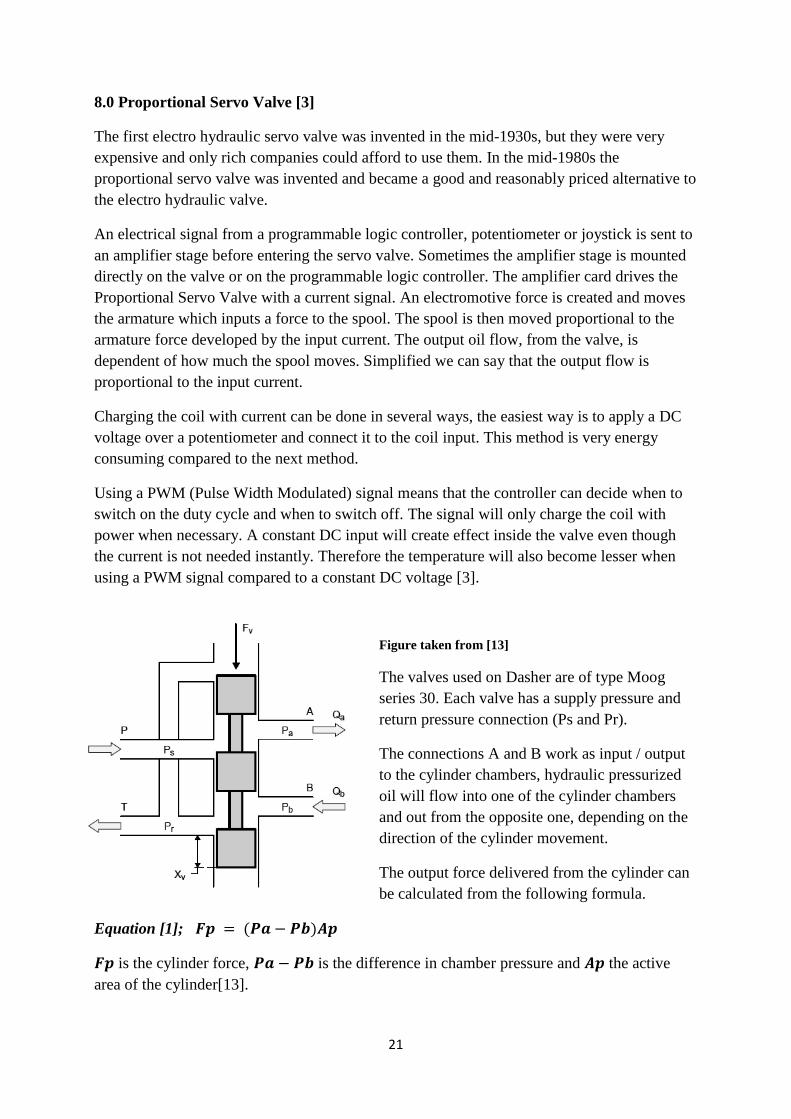
Figure taken from [13]
The valves used on Dasher are of type Moog
series 30. Each valve has a supply pressure and
return pressure connection (Ps and Pr).
The connections A and B work as input / output
to the cylinder chambers, hydraulic pressurized
oil will flow into one of the cylinder chambers
and out from the opposite one, depending on the
direction of the cylinder movement.
The output force delivered from the cylinder can
be calculated from the following formula.
Equation [1]; 𝑭𝒑 = (𝑷𝒂 − 𝑷𝒃)𝑨𝒑
𝑭𝒑 is the cylinder force, 𝑷𝒂 − 𝑷𝒃 is the difference in chamber pressure and 𝑨𝒑 the active
area of the cylinder[13].

22
9.0 Control Theory
Control theory is about automatizing a physical or an electronic process. No human being
needs to watch over the system, it will watch over itself. Nowadays we are surrounded by
controllers everywhere; it can be the temperature control-loop inside our house or the air-
conditioning system inside our car.
From control theory, we know that one of the easiest ways of controlling a system is to look at
the systems transfer function and calculate the controller parameters from that function. In
order to find the transfer function it is necessary to know the differential equation describing
the system mathematically, this is very hard to find for complex systems.
Dasher is a very complex robot, different subsystems work together and therefore the transfer
functions for Dasher is very hard to find. Each sub system must be regulated by a controller
and therefore approximations of the transfer functions must be made [12][16].
A typical control loop looks like figure 9.1. An input value is sent from a digital signal
processor or a potentiometer. The input value x will be compared with the sensor output value
r. If these two values are equal then the difference will be zero, no error signal e will be sent
to the controller. If x and r are not equal an error signal e will be sent to the controller. The
controller will input the error signal to the control algorithm and output the steering signal to
the process. The control algorithm is usually of type P, PI or PID where P equals the
proportional term, I the integrating term and D the derivative term.
Most controllers used in automatic processes are PI or PID controllers, simplified we can say
that the P term is the gain and speed of the controller, the I-term eliminates the stationary
error and the D term makes the controller more aware of rapid changes in signal input. The
PID controller is seen as the best controller to use in most applications, but still it depends on
the systems complexity, sometimes it is not necessary to use all three terms, many
applications work fine with only a PI controller [12][16].
Figure 9.0
23
𝑈 𝑡 = 𝐾𝑝𝑒 𝑡 + 𝐾𝑖 𝑒 𝑡 𝑑𝑡 + 𝐾𝑑
𝑑𝑒 𝑡
𝑑𝑡
Equation 2
The mathematical formula for a PID controller is shown in equation 2. Kp, Ki, Kd are the
controller gains. They are calculated from the transfer function of the physical system and
implemented in the controller algorithm (equation 9.1).
𝑈 𝑛 = 𝐾𝑝𝑒 𝑛 + 𝐾𝑖 𝑒(𝑘)
𝑛
𝑘=0
+ 𝐾𝑑(𝑦 𝑛 − 𝑦 𝑛 − 1 )
Equation 3
The control loop algorithm can also be expressed digitally (equation 3). Instead of
integration the formula uses a summation function and the derivative term is replaced by a
difference function. This formula can be used when programming a digital controller in
VHDL for instance.
If we consider the fact that the differential equation describing Dashers complexity is hard to
calculate by hand, then it might be easier to make a mathematical model in Matlab Simulink.
Simulink can simulate different scenarios and test different control loop parameters. It will be
easier to determine the optimal controller gains (Kp, Ki, Kd) for the controller compared to
calculating it by hand.
In those cases where a satisfying mathematical model of the system cannot be found,
experimental tuning of the control loop must be carried out then the following method is
commonly used[12][16].
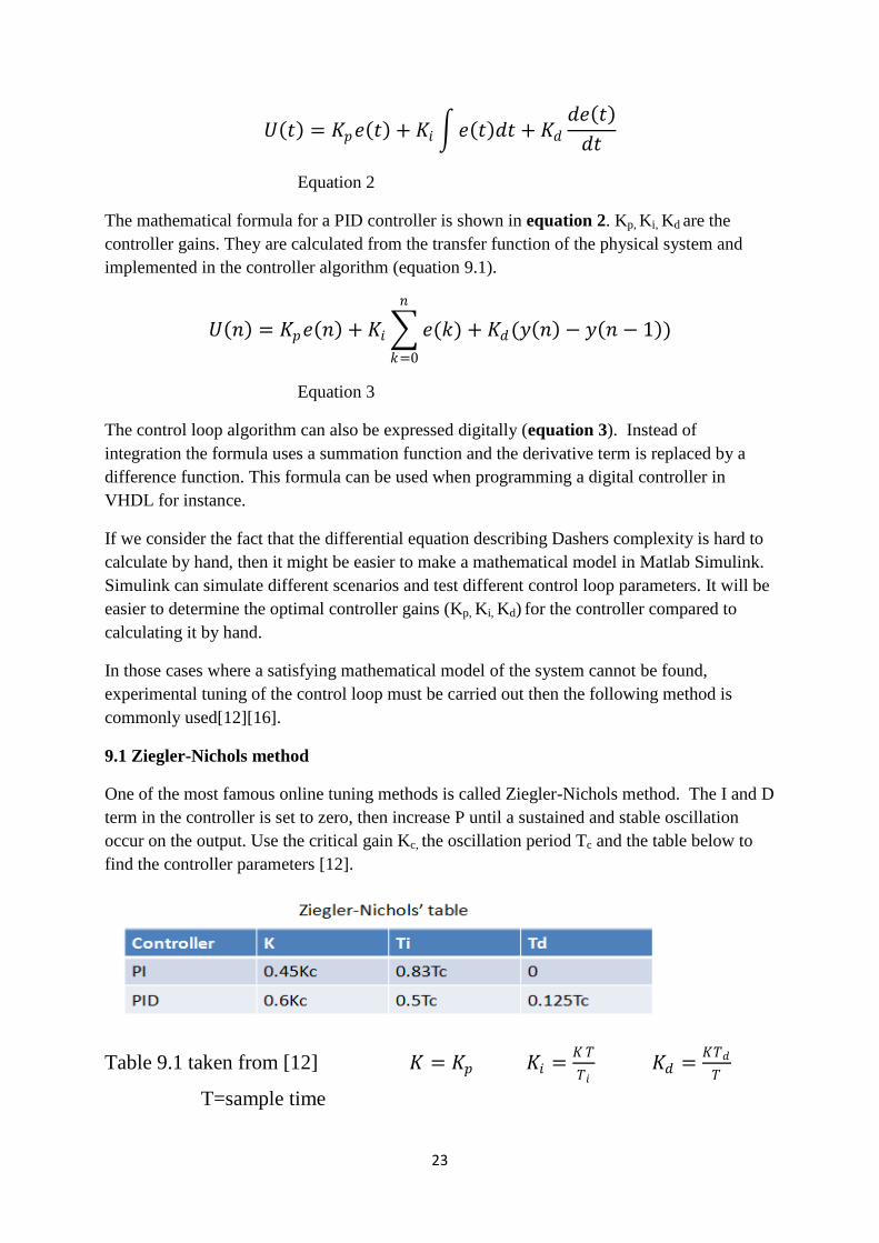
9.1 Ziegler-Nichols method
One of the most famous online tuning methods is called Ziegler-Nichols method. The I and D
term in the controller is set to zero, then increase P until a sustained and stable oscillation
occur on the output. Use the critical gain Kc, the oscillation period Tc and the table below to
find the controller parameters [12].
Table 9.1 taken from [12] 𝐾 = 𝐾𝑝 𝐾𝑖 =𝐾 𝑇
𝑇𝑖 𝐾𝑑 =
𝐾𝑇𝑑
𝑇
T=sample time
24
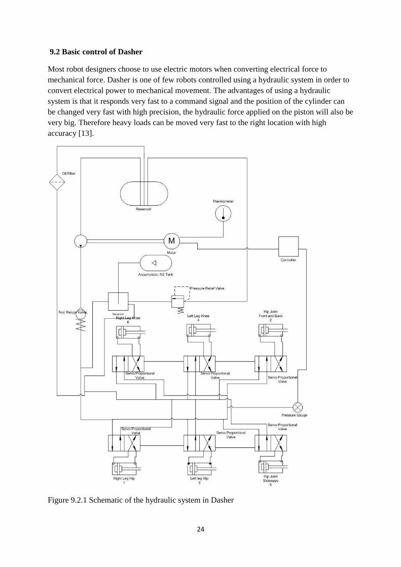
9.2 Basic control of Dasher
Most robot designers choose to use electric motors when converting electrical force to
mechanical force. Dasher is one of few robots controlled using a hydraulic system in order to
convert electrical power to mechanical movement. The advantages of using a hydraulic
system is that it responds very fast to a command signal and the position of the cylinder can
be changed very fast with high precision, the hydraulic force applied on the piston will also be
very big. Therefore heavy loads can be moved very fast to the right location with high
accuracy [13].
Figure 9.2.1 Schematic of the hydraulic system in Dasher

25
The hydraulic systems consist of a powerful brushless DC motor which runs a pump in high
speed. The pump pumps oil to the entire system and in order to build up hydraulic pressure
the oil will pass a non return valve immediately after leaving the pump. A reservoir filled with
nitrogen gas works as a pressure capacitor and will help maintaining a constant pressure and
eliminate fluctuations in oil pressure. The pressure capacitor is also used when setting the
system pressure at 100-200Bars. The system is capable of operating under 200Bars pressure
but will mostly operate under 100Bars pressure.
Figure 2.2.2
In order to lower the “center of mass point” on
Dasher the proportional valves, the cylinders and
the sensors will be assembled inside Dashers
legs. This design will make the position control
of the piston better. Less trapped oil between the
valve and the cylinder improves the performance
of the control loop and eliminates death band
and spring effect created by oil trapped between
the valve and the cylinder chamber.
The oil flow from the valve is controlled using
two PWM signals, PWM0 and PWM1. The
PWM signals work in opposite ways. When the
cylinder must move to the right, then PWM0
will tell the valve to increase the oil flow to
chamber A. When the cylinder must move to
left, PWM1 will switch on the oil flow to
chamber B instead.
In order to keep the leg in a fixed position
PWM0 and PWM1 continuously increase or decrease the oil flow to chamber A or B, which
prevents the leg from moving out of range from the set point. The gravity will try to force the
leg downwards and the controller needs to compensate for that movement by setting a correct
duty cycle on the appropriate PWM signal.
Figure 9.2.3
26
9.3 Position servos
Regarding the choice of controller type for the hydraulic control algorithm it might be easy to
say that a PID controller is the best choice. But if we consider that the hydraulic cylinder has
an integrating effect on the input signal, we may be able to use a simpler controller. We
already know that the stationary error will be zero even though we only use a P controller.
The input to the cylinder is the oil flow and the output is the integral of oil flow, which is the
change in position in x direction (according to figure 9.2.3).
The hydraulic cylinder works as a “position servo”, and in control theory position servos have
integrating effect on the input signal. The characteristic for a position servo is that the output
signal doesn’t have to be zero even though the input signal is. Some typical position servos
are elevators, robot arms and electrical motors. It is still useful to have integrating effect in the
controller, if a load is added to the cylinder, without integrating effect inside the controller;
we might get a stationary error because of the “load disturbance”. So using an I-term in the
controller is always useful even though the system has integrating effect already [12].
10.0 Simulink model
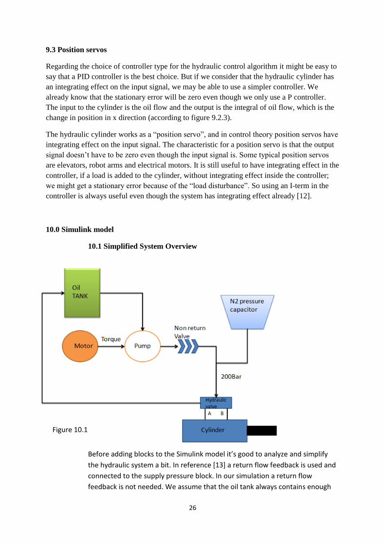
10.1 Simplified System Overview
Before adding blocks to the Simulink model it’s good to analyze and simplify
the hydraulic system a bit. In reference [13] a return flow feedback is used and
connected to the supply pressure block. In our simulation a return flow
feedback is not needed. We assume that the oil tank always contains enough
Figure 10.1

27
oil to run the pump and the motor will not be affected by fluctuations in return
pressure to the tank. The maximum system pressure is 200 bars. In the
Simulink model the Oil tank, Motor, Pump, non return valve and N2 pressure
capacitor will be simplified and modeled as a supply pressure block Ps. Ps will
be in Pascal (200 bars is 2.0e7 Pascal).
10.2 Simulink block layout [13]
In order to find the appropriate values for the controller parameters but also to simulate
different physical scenarios it’s good to make a Simulink model of the hydraulic system. This
model simulates the control of a Proportional Servo Valve connected to an actuator. The
model consists of controller which sends in an electric signal to the servo valve. The servo
valve will respond and send out an oil flow to Chamber A or B. The difference in oil flow to
the chambers results in a pressure difference, the pressure difference will create a force
moving the actuator in certain direction.
The following pages will described each block in the model and also the mathematical
formulas used to calculate the different parameters. The simulation result is presented in
the end of the model where the appropriate controller gains are calculated.
The effective area of chamber B is 𝐴𝐵 =𝜋
4(𝐷2 − 𝑑2) Equation 4
Figure 10.2 Hydraulic modeling in Simulink

28
Since the volume of chamber A and B are not equal (due to the piston in chamber B) the
following formula (Eq 4) can be used when calculating the percental difference in volume.
This percental difference is used as a constant in the valve block when calculating the flow
from chamber B.
10.3 Proportional servo valve block layout [13]
The proportional servo valve block has four input signals. Uv is the input voltage from the
controller. Pa and Pb are the feedback pressures from chamber A and B. Ps is the system
supply pressure. The block is divided into two major parts, the electrical dynamics and the
hydraulic dynamics. The upper part of the block diagram simulates the electrical dynamic and
the lower part the hydraulic. The following pages describe the mathematical function of the
servo valve and the physical parameters which are taken into account when modeling the
valve.
Figure 10.3 Proportional servo valve block layout
29
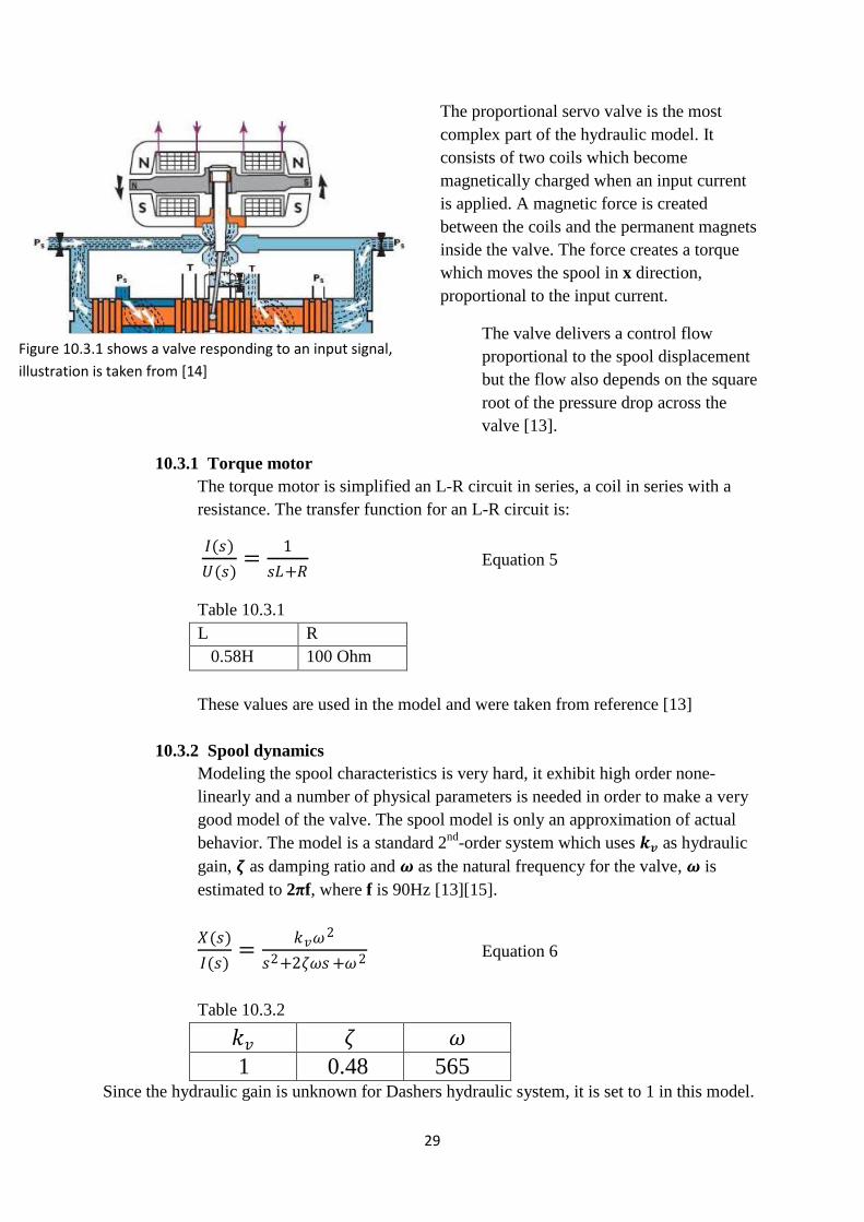
Figure 10.3.1 shows a valve responding to an input signal,
illustration is taken from [14]
The proportional servo valve is the most
complex part of the hydraulic model. It
consists of two coils which become
magnetically charged when an input current
is applied. A magnetic force is created
between the coils and the permanent magnets
inside the valve. The force creates a torque
which moves the spool in x direction,
proportional to the input current.
The valve delivers a control flow
proportional to the spool displacement
but the flow also depends on the square
root of the pressure drop across the
valve [13].
10.3.1 Torque motor
The torque motor is simplified an L-R circuit in series, a coil in series with a
resistance. The transfer function for an L-R circuit is:
𝐼(𝑠)
𝑈(𝑠)=
1
𝑠𝐿+𝑅 Equation 5
Table 10.3.1
L R
0.58H 100 Ohm
These values are used in the model and were taken from reference [13]
10.3.2 Spool dynamics
Modeling the spool characteristics is very hard, it exhibit high order none-
linearly and a number of physical parameters is needed in order to make a very
good model of the valve. The spool model is only an approximation of actual
behavior. The model is a standard 2nd
-order system which uses 𝒌𝒗 as hydraulic
gain, 𝜻 as damping ratio and 𝝎 as the natural frequency for the valve, 𝝎 is
estimated to 2πf, where f is 90Hz [13][15].
𝑋(𝑠)
𝐼(𝑠)=
𝑘𝑣𝜔2
𝑠2+2𝜁𝜔𝑠+𝜔2 Equation 6
Table 10.3.2
𝑘𝑣 𝜁 𝜔
1 0.48 565 Since the hydraulic gain is unknown for Dashers hydraulic system, it is set to 1 in this model.

30
10.3.3 Flow continuity function
For varying loads, the control flow is proportional to the square root of the
pressure drop over the valve. The following equation is a rough approximation
of the flow continuity function in [13], for example current Iv is used in the
equation in [13] but since it’s not clear from the reference where to use Iv in the
Simulink model (except from when calculating spool position x) Iv is ignored.
The following equation is used 𝑄𝐿 = 𝑄𝑅 ∗ 𝑥 ∗ Δ𝑃𝑣
Δ𝑃𝑅 equation 7
Where Δ𝑃𝑣 = 𝑃𝑆 − 𝑃𝑇 − 𝑃𝐿 and Δ𝑃𝑅 = 𝑃𝑆 − 𝑃𝑇 − 𝑃𝑎
Δ𝑃𝑣 = Pressure drop over the valve
Ps=supply pressure, PT= return pressure to tank, PL=load pressure
Pa is a constant taken from [13] and the value is 6.89e6 Pascal. It is used when
calculating rated valve pressure across connections A and B [13].
10.4 Model of the hydraulic cylinder [13]
Section 10.4 describes how to model the hydraulic cylinder mathematically in
Simulink.
31
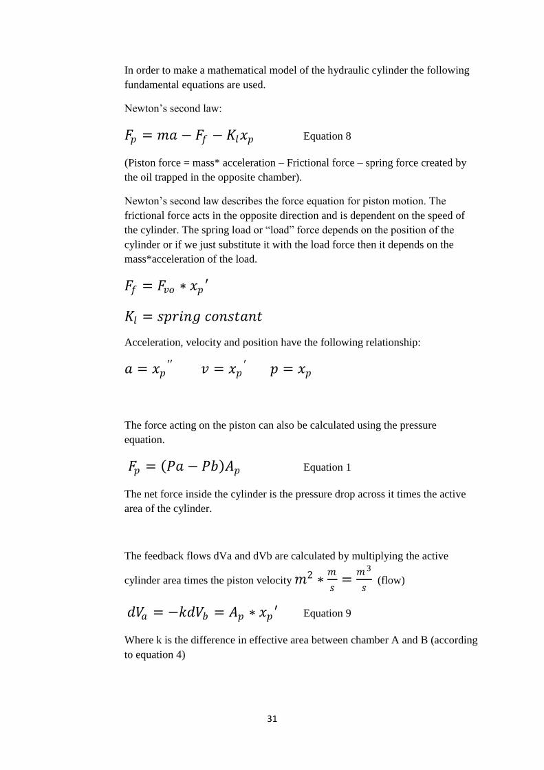
In order to make a mathematical model of the hydraulic cylinder the following
fundamental equations are used.
Newton’s second law:
𝐹𝑝 = 𝑚𝑎 − 𝐹𝑓 − 𝐾𝑙𝑥𝑝 Equation 8
(Piston force = mass* acceleration – Frictional force – spring force created by
the oil trapped in the opposite chamber).
Newton’s second law describes the force equation for piston motion. The
frictional force acts in the opposite direction and is dependent on the speed of
the cylinder. The spring load or “load” force depends on the position of the
cylinder or if we just substitute it with the load force then it depends on the
mass*acceleration of the load.
𝐹𝑓 = 𝐹𝑣𝑜 ∗ 𝑥𝑝 ′
𝐾𝑙 = 𝑠𝑝𝑟𝑖𝑛𝑔 𝑐𝑜𝑛𝑠𝑡𝑎𝑛𝑡
Acceleration, velocity and position have the following relationship:
𝑎 = 𝑥𝑝′′ 𝑣 = 𝑥𝑝
′ 𝑝 = 𝑥𝑝
The force acting on the piston can also be calculated using the pressure
equation.
𝐹𝑝 = 𝑃𝑎 − 𝑃𝑏 𝐴𝑝 Equation 1
The net force inside the cylinder is the pressure drop across it times the active
area of the cylinder.
The feedback flows dVa and dVb are calculated by multiplying the active
cylinder area times the piston velocity 𝑚2 ∗𝑚
𝑠=
𝑚3
𝑠 (flow)
𝑑𝑉𝑎 = −𝑘𝑑𝑉𝑏 = 𝐴𝑝 ∗ 𝑥𝑝 ′ Equation 9
Where k is the difference in effective area between chamber A and B (according
to equation 4)

32
10.5 Flow to pressure conversion inside chamber A or B [13]
Simulink Modeling
The following equation is used in fluid mechanics to express the relationship
between control flow and pressure inside a chamber.
Σ𝑄𝑖𝑛 − Σ𝑄𝑜𝑢𝑡 =𝑑𝑉
𝑑𝑡+
𝑉
𝛽
𝑑𝑃
𝑑𝑡
The equation can be rearranged to express pressure inside chamber A or B
𝑃𝐴 =𝛽
𝑉 (𝑄𝐴 −
𝑑𝑉𝐴
𝑑𝑡)𝑑𝑡 Equation 10
𝛽=bulk modulus for mineral oil 1.4*109 N/m
2
𝑉= volume of trapped oil between pump and servo valve
The sensor is a slide potentiometer (fig 7.2.3) which converts position to
voltage; 0-5V corresponds to 0-10cm in stroke.
10.6 Sensor block
10.7 Controller block layout

33
The following m.file loads the model with the system parameters
clear all close all clc
global Ivsat Qr Pt beta Kl Ap Fco Fvo Ps Mp PID_Kp PID_Ki PID_Kd;
beta=1.4*10e9; %Pascal bulk modulus constant; Ap=0.0007; %m2 active area of the cylinder must be quite high to Ivsat=0.02; %A valve saturation current Pt=1.0e6; %Pascal return pressure Ps=2.1e7; %Pascal supply pressure Mp=1; %kg mass of cylinder Qr=0.00063; %m3/s rated flow Kl=60; % spring constant Fvo=100; % friction constant
(Some values are taken from [13] while the others are estimated)
10.8 Simulation results
Fig: 10.8.1
%****Controller gains*******
PID_Kp=9;
PID_Ki=0;
PID_Kd=0;
%***************************
According to the simulation result (fig 10.8.1) a controller armed with these values (Kp=9
Ki=0 Kd =0) is optimal. The over shoot is very small and the slew rate very fast. Normally we
need a Ki term (integration) to eliminate the stationary error but since the hydraulic cylinder
have automatically integration inside chamber A and B a Ki term is not necessary. Only if a
stationary force is applied externally we might get a stationary error without integration in the
controller. Therefore when running the robot it’s very good to have integration inside the
controller too.

34
This model is just an approximation of actual system behavior we must take into account that
all system parameters might not be correct. The friction force coefficient is unknown for the
pistons used on the robot, but is estimated to approximately 60N in the Simulink model.
Below are some graphs showing the behavior of output response if the friction force is
changed.
Fig 10.8.2 Low friction
If the friction force is too low, the system tends to become more unstable because very little
energy is necessary to accelerate the piston (Fvo=30; %friction)
Fig 10.8.3 High friction
High friction increases the overshoot, more energy is necessary in order to move the cylinder.
Once the threshold force is overcome it takes longer time for the controller to compensate that
force and that’s why the overshoot is larger; this is more preferable though than low friction
behavior. (Fvo=600; %friction)

35
10.9 Motion simulation
After tuning the controller it was of interest to see what happens if the load is
changed. Simplified a load could be added to the piston and the result could be
plotted but this thesis has chosen another more interesting approach. Instead of
just a load at the end of the piston the following chapter will simulate the forces
created inside Dasher’s leg while executing a running motion for various loads.
This model is just an approximation of actual behavior there are a lot more
physical parameters which affects the leg while running; the report only uses the
most important once.
In the model of the hydraulic cylinder there is a hydraulic spring parameter Kl,
if we substitute Kl with a Matlab function block, we can simulate the force
acting on the piston for different loads.
<
E
x
p
l
a
i
Since we want to simulate both thigh and knee in this model we put the math
function outside this block and duplicate the system (as shown in figure 10.9.1)
and name them thigh and knee. The sub systems contain a copy of the hydraulic
servo valve model explained above
(10.2). The input values to the
function are the position of the
pistons.
In order to write the m.file to the
function block a mathematical
model of the forces acting inside
the legs need to be done. The
gravity will play a big role when
modeling the force equations.
Figure 10.9.1

36
The function utilizes the length of the piston to calculate the necessary force
inside the hydraulic cylinder, in order to lift the leg. The main idea is to
calculate the force using the Torque equation for different angels.
Force model of the thigh Figure 10.9.2
The figure (10.9.2) shows how the leg is assembled and how the force will act
on the piston for different angels; from this model we can write the
mathematical formulas needed to calculate the force. The following equations
are used when calculating the force needed to lift the thigh.
Length:
The length of c is calculated using Pythagoras theorem.
C = a2 − d2 Equation (11)
Angels:
The angels are calculated using the cosine law and cosine function.
𝛽 = arccos( 𝑐
𝑎 )
Φ = arccos( −(𝐹2−𝑎2−𝑏2)
2𝑎𝑏 ) Equation (12)
𝛿 =𝜋
2+ 𝛽 − Φ
𝜇 = arccos 𝑑
𝑎 ω = arccos
–(𝑏2−𝐹2−𝑎2)
2𝑎𝐹
𝛾 = 𝜇–ω
37
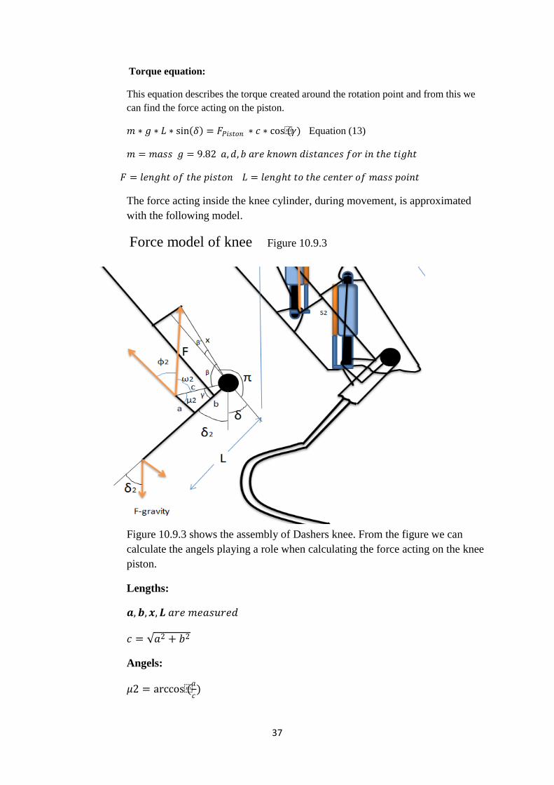
Torque equation:
This equation describes the torque created around the rotation point and from this we
can find the force acting on the piston.
𝑚 ∗ 𝑔 ∗ 𝐿 ∗ sin 𝛿 = 𝐹𝑃𝑖𝑠𝑡𝑜𝑛 ∗ 𝑐 ∗ cos(𝛾) Equation (13)
𝑚 = 𝑚𝑎𝑠𝑠 𝑔 = 9.82 𝑎,𝑑, 𝑏 𝑎𝑟𝑒 𝑘𝑛𝑜𝑤𝑛 𝑑𝑖𝑠𝑡𝑎𝑛𝑐𝑒𝑠 𝑓𝑜𝑟 𝑖𝑛 𝑡𝑒 𝑡𝑖𝑔𝑡
𝐹 = 𝑙𝑒𝑛𝑔𝑡 𝑜𝑓 𝑡𝑒 𝑝𝑖𝑠𝑡𝑜𝑛 𝐿 = 𝑙𝑒𝑛𝑔𝑡 𝑡𝑜 𝑡𝑒 𝑐𝑒𝑛𝑡𝑒𝑟 𝑜𝑓 𝑚𝑎𝑠𝑠 𝑝𝑜𝑖𝑛𝑡
The force acting inside the knee cylinder, during movement, is approximated
with the following model.
Force model of knee Figure 10.9.3
Figure 10.9.3 shows the assembly of Dashers knee. From the figure we can
calculate the angels playing a role when calculating the force acting on the knee
piston.
Lengths:
𝒂,𝒃,𝒙,𝑳 𝑎𝑟𝑒 𝑚𝑒𝑎𝑠𝑢𝑟𝑒𝑑
𝑐 = 𝑎2 + 𝑏2
Angels:
𝜇2 = arccos(𝑎
𝑐)
38
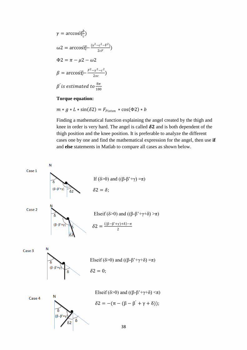
𝛾 = arccos(𝑏
𝑐)
ω2 = arccos(−(x2−c2−F2)
2𝑐𝐹)
Φ2 = 𝜋 − 𝜇2 − 𝜔2
𝛽 = arccos(−𝐹2−𝑥2−𝑐2
2𝑥𝑐)
𝛽′ 𝑖𝑠 𝑒𝑠𝑡𝑖𝑚𝑎𝑡𝑒𝑑 𝑡𝑜8𝜋
180
Torque equation:
𝑚 ∗ 𝑔 ∗ 𝐿 ∗ sin 𝛿2 = 𝐹𝑃𝑖𝑠𝑡𝑜𝑛 ∗ cos Φ2 ∗ 𝑏
Finding a mathematical function explaining the angel created by the thigh and
knee in order is very hard. The angel is called 𝜹𝟐 and is both dependent of the
thigh position and the knee position. It is preferable to analyze the different
cases one by one and find the mathematical expression for the angel, then use if
and else statements in Matlab to compare all cases as shown below.
If (δ>0) and ((β-β’+γ) =π)
𝛿2 = 𝛿;
Elseif (δ>0) and ((β-β’+γ+δ) >π)
𝛿2 = (β−β’+γ)+δ −𝜋
2
Elseif (δ>0) and ((β-β’+γ+δ) =π)
𝛿2 = 0;
Elseif (δ>0) and ((β-β’+γ+δ) <π)
𝛿2 = −(π − (β − β′ + γ + δ));

39
Elseif (δ=0) and ((β-β’+γ) =π)
𝛿2 = 0;
Elseif (δ=0) and ((β-β’+γ) <π)
𝛿2 = −(𝜋 − β − β’ + γ );
Elseif (δ<0) and ((β-β’+γ) =π)
𝛿2 = 𝛿;
Else
𝛿2 = 𝛿 − (𝜋 − ( β-β’+γ)));
Now when the model of the leg is finished and suitable mathematical equations have been
used it’s time to write the Matlab code. The following code is used in the Matlab function in
order to simulate Dasher’s leg during a running motion. The function will calculate the angel
of the thigh and knee by using the position of the pistons. It will take into account the weight
and the gravity force and calculate the force acting on the piston by using the torque equation.

40
Finally a plot function is implemented which plots a figure of the leg. The figure will show
visually how Dasher’s thigh and knee are executing a running motion.
The Matlab code can be found in Appendix A.
10.10 Motion simulation result
Plot 10.10.1: Shows how the gravity affects the step response of the controller
The gravity will force the leg
slightly downwards before the
controller responds to it. If we
compare this step response
with the previous one in 10.8
we can see that the overshoot
is eliminated as a result of the
gravity force which pulls the leg downwards. The more weight we add to the Simulink model
the more will the gravity will pull down the step response curve.
Plot 10.10.2 Thigh position compared to piston force when unloaded, mthigh=10kg
The length of the piston follows the systems input value very well (yellow and blue curves).
The green curve is the force created in hydraulic cylinder which controls the position of the
thigh. If the piston length is compared with the force, we can see that maximum positive force

41
is obtained when the piston length is 0 (which means that Dasher lifts his leg forward to its
maximum position).When the length of the piston is 3cm the leg passes the “sign of gravity
barrier” and the force will change sign (which means that Dashers thigh points backwards
instead of forward). For an unloaded Dasher we can see that the required force to move the
thigh in certain angels varies between -150 to 300 Newton.
Plot 10.10.3 Approximation of required force to lift Dasher’s entire mass (thigh)
Now when the Simulink model works it will be fun to estimate the required force to move
Dasher’s entire weight. If we consider Dasher standing on the floor with his entire body mass
of 50kg pointing downwards and his feed fixture to the floor then the simulation shows that
the maximum required force to move the thigh up and down is 1520N, but in order to move
that mass with high acceleration more force is needed (since force equals mass times
acceleration). Though this simulation is not fully accurate the result just gives an idea about
the required force.
Knee_____________________________________________________________________
Plot 10.10.4 Force in knee cylinder when unloaded (mass of knee 1kg)

42
Plot 10.10.4 shows the force required in the knee cylinder in order to move the knee when
Dasher is freely hanging in the air unloaded. The cylinder force only needs to overcome the
gravity force. The mass of the knee is approximately 1 kg and the maximum force varies from
47N to 63N.
Let’s pretend a load as big as Dasher’s entire weight (50kg) is hanged in his feet and a
running motion is simulated. The force in the knee cylinder will now be dependent on the
angel of the knee and the angel of the thigh. The following plot is obtained (10.10.5).
Plot 10.10.5 shows the knee piston force required during a running motion.
The Simulation shows that when the thigh is almost in its full upper position (position value
0) and the knee is in its front position (position value 5) then we obtain maximum positive
force in the knee cylinder (blue circle). Maximum negative force is more difficult. In this
simulation it is obtained when the thigh is in position (2.5) and the knee is in position (4). But
this combination can be changed to other combinations which gives the same result or even
more negative force. The force in the knee piston depends on the position of the knee as well
as the position of the thigh, the angels created inside the knee (according to the figure drawn
in 10.9) does also play a role. The force inside the knee cylinder varies between -5600N to
2000N in this example.

43
Plot (10.10.6) shows the visual simulation result of the running pattern plotted in (plot
10.10.5)
In reality a real simulation of a running motion would not look like this, the applied force
would be much smaller when the leg is not touching ground. The leg is only touching ground
on its way from the front position to the back position. That corresponds to 30% of the
periodic time. In this simulation the gravity is pulling the leg downwards to the ground which
gives the resulting force plotted in 10.10.5. In reality the force would have the opposite sign
when the weight is pressing the robot downwards. The force inside the cylinders needs to
press back the upper body in order to avoid the robot from falling down to the ground. It can
be compared with a real human leg. If we want to lift our body upwards then the front muscle
on our thigh works very hard. If we want to press our leg downwards against the ground while
running then the muscle on the backside of the thigh must work hard. This is similar to the
force acting inside the cylinder but with the opposite sign.

44
11.0 Result
11.1 The thesis work
A major problem during the project was the mechanical design. The mechanical structure did
not support the demands a running robots needs to fulfill. Maybe one disadvantage is that
several project groups have worked on this robot before, the mechanical group did not think
of the physical demands which the structure needs to live up to in order to work later on when
the electronics group is testing it. During my project, Dasher was continuously tested with
different control loop parameters but almost every time something broke and needed to be
repaired which took a lot of time. Before serious control theory experiments can be carried
out on Dasher the robot needs to be redesigned mechanically (in order to withstand all forces
acting on the structure during a test). Another delaying factor during the project was that we
were eight persons in the project group and at least 4 persons where depending on each
other’s achievements in order to make progress. Such achievements were programming and
debugging code, mechanical assembly, soldering and harness tasks. The experience level in
the group varied from person to person. Some work was carried out poorly, which led to
reparations and wasted time later on in the project.
Finally at the end of the project the main hydraulic engine broke, no more control theory
experiments could be carried out physically on the robot. The main task for me and my thesis
became to make a Simulink model which could simulate different scenarios. Suitable
controller gains could then be taken from the model and used in real tests on the robot.
11.2 Conclusions
The ambitions were very high when we started the project in March 2009, everyone in the
group seemed quite certain that the robot would make great progress during the project. The
goal was still, like for the previous project groups, to make Dasher run. Now when the project
period is finished, it’s clear that the goal was set very high and that it’s more important to take
small steps one by one in order to make progress in the project. Basic things like designing a
mechanical structure that handles the hydraulic forces and Dasher’s weight is important, the
sensors cannot be of poor quality they must handle vibrations and leaking oil and the noise
level must be very low.
The electronics must be assembled correctly, the node cards interfered each other if not
grounded properly. The control loop worked quite well when testing it onto the cylinders. A
position could be set and the piston moved to that position but oscillations around the set
point occurred due to the noise problem explained in (7.2). The engine broke before we had
time to test the new Alps sensors in (7.3). The main computer worked well in simulations but
when testing to control loop using the main computer as master and the node card as a slave,
the system became too slow, it had probably to do with some program bug.
The result in this report shows a method of calculating proper controller gains for the
controller. It also shows a simulation of the forces acting inside the cylinders when moving a
mass as big as Dasher. One reason of why the forces are so big inside the knee piston is the

45
design of it. The length between the two points is only 2cm while the length of the entire knee
is 48cm. The force equation gives a huge force inside the cylinder due to the difference in
length between length of the knee and the torque rotational point and the length between the
piston assembly points end the torque rotational point. In order to reduce the force, the length
between the knee assembly point and the torque rotational point must be longer and the angel
created between the piston and the assembly point must be changed. Ideally that angel should
be 90 degrees phase shifted with respect to the vertical hanging knee. Then the force created
inside the piston will be converted to pure torque without angular losses. It is of course
impossible to fit the pistons inside the leg in
that way but that would give the optimal
mechanical force conversion.
Future development of the robot must handle
the mechanical weakness of the structure, the
weight should be reduced and the knee piston
should be assembled in another way that gives
more torque for less amount of power. When
the mechanical structure is done then it will be
easier to carry out control theory test on the
robot.
Torque rotational point
46
References
Internet
[1] Industrialismen http://skolarbete.nu/skolarbeten/industrialismen/
[2] Dasher http://www.idt.mdh.se/rc/Dasher/
[3] Proportional and Servo Valve Technology, Fluid Power Journal March/April
2003 http://www.scribd.com/doc/13981238/Proportional-and-Servo-Hydraulic-
Valve-Primer-
[4] http://en.wikipedia.org/wiki/Industrial_Revolution
Document
[11] Dasher a running robot, Carried out under the supervision of
Prof. Lars Asplund at Mälardalens Högskola Submitted for the fulfillment of
ROBOTICS COURSE (CDT508) By
Sundara Vadivel Kumar
Praveen Vikram
Harsha Atluri
Rohit Jayadevan
Ajay Ravichandran
Deepak Krishnamurthy
Navneet Menon
Sandeep Kottath [email protected]
[12] Processreglering
av Lennart Harnefors, tillämpad Signal Och Reglerteknik
Institutionen För Elektronik
Mälardalens högskola 4 november 2002
[13] DSP Control of Electro-Hydraulic Servo Actuators, Application Report SPRAA76–January 2005 by Texas Instruments Richard Poley
[14] Electro hydraulic valves a technical look, MOOG, Industrial control Division
[15] TRANSFER FUNCTIONS FOR MOOG SERVOVALVES, W. J. THAYER,
DECEMBER 1958. Rev. JANUARY 1965
[16] Implementation of PID and Dead beat Controllers with theTMS320
Family. APPLICATION REPORT: SPRA083 Irfan Ahmed Digital Signal Processor
Products Semiconductor Group Texas Instruments

47
Appendix A
Matlab function that calculates the force inside the pistons
------------------------------------------------------------
function out=Leng2Force(input); % clc
F=input(1)+17.5; F1=input(2)+14;
%Thigh%%%%%%%%%%%%%%%%%%%%%%%%%%%%%%%%% a=20; b=4; d=4; M=10; L=28; g=9.8;
c=sqrt(a^2-d^2); beta=acos(c/a); phi=acos((-(F^2-a^2-b^2))/(2*a*b)); delta=pi/2+beta-phi; gamma=acos(d/a)-acos((-(b^2-F^2-a^2))/(2*a*F)); FF=(M*g*L*sin(delta))/(c*cos(gamma)); %--------------------------------------
%----------Knee------------------------ a1=3; b1=5;
x1=10; L1=20; M1=2; %------------------ %-------------------------------------- c1=sqrt(a1^2+b1^2); micro=acos(a1/c1); omega=acos((-(x1^2-c1^2-F1^2))/(2*c1*F1)); phi1=pi-micro-omega; %%%%%%%%%%%%% beta1=acos((-(F1^2-x1^2-c1^2))/(2*x1*c1)); Bprim=(8*pi)/180; gamma1=acos(b1/c1);
%%%%delta1=pi+Bprim-beta1-gamma1-delta;
%case1 if (delta>0)&&((beta1-Bprim+gamma1)==pi)
delta2=delta;
%case2 elseif (delta>0)&&((beta1-Bprim+delta+gamma1)<pi)
delta2=beta1-Bprim+delta+gamma1-pi;
48
%case 3 elseif (delta>0)&&((beta1-Bprim+delta+gamma1)==pi) delta2=0; %case 4 elseif (delta>0)&&((beta1-Bprim+gamma1+delta)<pi) delta2=-(pi-(beta1-Bprim+gamma1+delta));
%case 5 elseif (delta==0)&&((beta1-Bprim+gamma1)==pi) delta2=0;
%case 6 elseif (delta==0)&&((beta1-Bprim+gamma1)<pi) delta2=-(pi-(beta1-Bprim1+gamma1)); %case 7 elseif (delta<0)&&((beta1-Bprim+gamma1)==pi) delta2=delta;
else delta2=-(delta+(pi-(beta1-Bprim+gamma))); end
%%%%%%%%%%%%%% FF1=(M1*g*L1*sin(delta2))/(b1*cos(phi1));
out=[FF FF1];
--------------------------------------------------------------------------------------------------------------
Plot function, which creates an animated leg that simulate actual behavior
------ PLOT ------
S=70; plot([0 0],[-S S],'g-'); hold on plot([-S S],[0 0],'g-'); hold on
plot(0,0,'bo');
plot([0 b],[0 0],'b-'); hold on
fi=delta+(3*pi/2); %fi=phi-pi/2; R=[cos(fi) -sin(fi); sin(fi) cos(fi)];
p=R*[L 0]'; plot([0 p(1)],[0 p(2)],'b-');
pa=R*[a 0]'; pd=R*[a -d]'; plot([pa(1) pd(1)],[pa(2) pd(2)],'b-');
plot([0 pd(1)],[0 pd(2)],'r-');

49
plot([b pd(1)],[0 pd(2)],'r-');
---------------------------------------
p1=R*[L-b1 0]'; p2=R*[L-b1 a1]'; plot([p1(1) p2(1)],[p1(2) p2(2)],'b-');
p1=R*[L 0]'; p2=R*[L b1]'; plot([p1(1) p2(1)],[p1(2) p2(2)],'b-'); plot(p2(1),p2(2),'bo');
fi1=delta2; R1=[cos(fi1) -sin(fi1); sin(fi1) cos(fi1)];
p1=R*R1*[L1 0]'+p2; plot([p1(1) p2(1)],[p1(2) p2(2)],'b-');
p3=R*R1*[L1 8]'+p2; plot([p1(1) p3(1)],[p1(2) p3(2)],'b-');
p1=R*R1*[b1 0]'+p2; p2=R*R1*[b1 -c1]'+p2; plot([p1(1) p2(1)],[p1(2) p2(2)],'b-');
p1=R*[L-b1 a1]'; plot([p1(1) p2(1)],[p1(2) p2(2)],'r-');
axis([-S S -S S]) axis equal drawnow; hold off
end
------------------------------------------------------------------------------------------------


