Circulant and Elliptic Feedback Delay Networks for Artificial Reverberation Davide Rocchesso, Julius O. Smith * Abstract The feedback delay network (FDN) has been proposed for digital reverberation. Also pro- posed with similar advantages is the digital waveguide network (DWN). This paper notes that the commonly used FDN with an N × N orthogonal feedback matrix is isomorphic to a normal- ized digital waveguide network consisting of one scattering junction and a vector transformer joining N reflectively terminated branches. Generalizations of FDNs and DWNs are discussed. The general case of a losslessness FDN feedback matrix is shown to be any matrix having unit-modulus eigenvalues and linearly independent eigenvectors. A special class of FDNs using circulant matrices is proposed. These structures can be efficiently implemented and allow con- trol of the time and frequency behavior. Applications of circulant feedback delay networks in audio signal processing are discussed. Contents 1 Introduction 3 1.1 Prior Work ......................................... 3 1.2 Lossless Reveberator Prototypes ............................. 4 1.3 Summary and Outline ................................... 4 2 Feedback Delay Networks 4 3 Digital Waveguide Networks 8 3.1 Lossless Scattering ..................................... 9 3.2 Normalized Scattering ................................... 10 3.3 Complexity ......................................... 10 3.4 Conditions for Losslessness ................................ 10 3.5 Relation of DWNs to FDNs ................................ 11 3.6 Finite-Wordlength Effects ................................. 13 * D. Rocchesso is with the Centro di Sonologia Computazionale, Dipartimento di Elettronica e Informatica, Uni- versit` a degli Studi di Padova, via Gradenigo, 6/A - 35131 PADOVA - ITALY, Phone: ++39+49.8283757, FAX: ++39+49.8287699, E-mail: [email protected]. J. O. Smith is with the Center for Computer Research in Music and Acoustics (CCRMA), Music Department, Stanford University, Stanford, CA 94305, E-mail: [email protected]. 1
Transcript
Circulant and Elliptic Feedback Delay Networks for Artificial
Reverberation
Davide Rocchesso, Julius O. Smith∗
Abstract
The feedback delay network (FDN) has been proposed for digital reverberation. Also pro-posed with similar advantages is the digital waveguide network (DWN). This paper notes thatthe commonly used FDN with an N ×N orthogonal feedback matrix is isomorphic to a normal-ized digital waveguide network consisting of one scattering junction and a vector transformerjoining N reflectively terminated branches. Generalizations of FDNs and DWNs are discussed.The general case of a losslessness FDN feedback matrix is shown to be any matrix havingunit-modulus eigenvalues and linearly independent eigenvectors. A special class of FDNs usingcirculant matrices is proposed. These structures can be efficiently implemented and allow con-trol of the time and frequency behavior. Applications of circulant feedback delay networks inaudio signal processing are discussed.
∗D. Rocchesso is with the Centro di Sonologia Computazionale, Dipartimento di Elettronica e Informatica, Uni-versita degli Studi di Padova, via Gradenigo, 6/A - 35131 PADOVA - ITALY, Phone: ++39+49.8283757, FAX:++39+49.8287699, E-mail: [email protected]. J. O. Smith is with the Center for Computer Research in Music andAcoustics (CCRMA), Music Department, Stanford University, Stanford, CA 94305, E-mail: [email protected].
Artificial reverberation is a challenging application in signal processing because it is necessary toapproximate large systems (such as concert halls) having hundreds of thousands of poles and zeros inthe audio band. Instead of pursuing explicit models which are prohibitively complex, it is necessaryto find alternative abstractions which can be implemented at reasonable cost and which capture thesalient psychoacoustical attributes of natural reverberation. An important practical requirement isa stable numerical implementation of sparse, high-order, nearly lossless linear systems. This paperaddresses this and related issues.
1.1 Prior Work
The field of digital artificial reverberation was launched by M. Schroeder more than thirty yearsago [25]. In his pioneering work, he introduced recursive comb filters and allpass filters as suitablemeans for inexpensive simulation of multiple echoes. In particular, he introduced use of allpassfilters of the form y(n) = gx(n)+x(n−N)− gy(n−N), with N any positive integer, for achievingdense echoes with a flat amplitude response. This structure has since been used extensively inartificial reverberation [16].
In the seventies, M. A. Gerzon [4] generalized the single-input, single-output Schroeder allpassto M inputs and outputs by replacing the N -sample delay line with an order M “unitary network”(a square matrix transfer function having a frequency response matrix which is a unitary matrixat all frequencies, i.e., it must be a “paraunitary” transfer function matrix [31]).
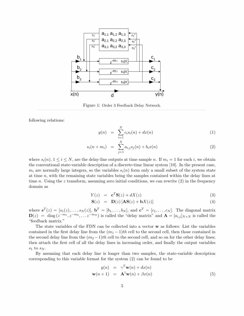
J. Stautner and M. Puckette [30] introduced what we now call feedback delay networks (FDNs)as structures well suited for artificial reverberation. These structures are characterized by a set ofdelay lines connected in a feedback loop through a “feedback matrix” (see Fig. Fig. 1). The FDNwas obtained as a generalization of the recursive feedback comb filter y(n) = x(n−N)+ gy(n−N)by (1) replacing the single N -sample delay line by a diagonal matrix of delay lines of differentlengths, and (2) replacing the feedback gain g by the matrix G = UD, where U is any unitarymatrix,1 and D is any diagonal matrix having all elements less than 1 − ε in magnitude, whereε > 0 determines the stability margin. Specific early reflections were implemented by adding scaledcopies of the source signal into selected points along the delay lines, corresponding to use of thetransposed form of the FIR filter [19]. Early reflections in artificial reverberation were apparentlyfirst implemented by J. A. Moorer using a direct-form FIR filter in series with Schroeder allpassfilters and air-absorption comb filters [16].
More recently, J. M. Jot has extensively studied FDNs and developed associated techniques fordesigning good quality reverberators. He suggested the use of efficient special cases of unitary feed-back matrices as well as techniques for pole-placement to obtain a desired decay-time vs. frequency[8], and introduced the valuable design principle that, for smoothest (idealized) late reverberation,all modes in a given frequency band should decay at substantially the same rate in order to avoidisolated ringing modes in the late reverberation which tend to sound “metallic” [9].
In 1986, digital waveguide networks (DWN) were proposed as a useful starting point for digitalreverberator design [26]. The idea was to build an arbitrary closed network of digital waveguidesexhibiting the desired early reflections and late echo density, and then introduce loss filters intothe network to achieve the desired decay time vs. frequency. Approaching reverberation via lossless
1While papers on this subject speak of unitary feedback matrices U ∈ CN defined by UHU = I, where UH denotes
the Hermitian transpose of U , all practical applications thus far appear to be confined to orthogonal matrices U ∈ RN .
3
prototypes leads to good numerical and stability properties [27, 31]. Like FDNs, DWNs make iteasy to construct well-behaved, high-order, nearly lossless systems.
1.2 Lossless Reveberator Prototypes
Reverberator design is often factored into separate designs of the early reflections and the late“diffuse” reverberation. Specific early reflections are easily realized using FIR filter taps. To de-velop a high quality late reverberation, it is good to begin with a lossless prototype reverberatorso that the structure of its late time response can be clearly heard. Nominally, a lossless prototypereverberator is judged by the quality of white noise it generates in response to an impulse signal.For smooth late reverberation, the white noise should sound uniform in every respect. Subsequentintroduction of sparse lowpass filters into the prototype network serves to set the desired reverber-ation time vs. frequency. In other words, starting with lossless networks allows the decoupling ofreverberation time from structural aspects of the reverberator. Any “passive” arithmetic scheme,such as magnitude truncation, can be used at certain multiplier outputs to eliminate the possibilityof limit cycles and overflow oscillations [27].
Since FDNs and DWNs appear to present very different approaches for constructing losslessreverberator prototypes, it is natural to ask what connections may exist between them, and whetherthere may be unique advantages of one over the other.
1.3 Summary and Outline
In section II, we briefly review the FDN and discuss some of its algebraic properties. In section III,we explore connections between FDNs and DWNs: It is shown how a single-junction DWN createdby the intersection of N waveguides can be interpreted as an order N FDN; conversely, it is shownthat any FDN can be interpreted as a DWN, although its scattering junction is not necessarilyphysical. We derive general conditions for lossless FDN feedback matrices in which the unitarymatrix normally used in FDNs is extended to any matrix having unit-modulus eigenvalues andlinearly independent eigenvectors. The extension corresponds to a generalization of signal energyby replacing the L2 norm with an elliptic norm induced by any Hermitian, positive-definite matrix[20]. In section IV, circulant matrices are proposed as good choices for FDNs due to their efficiencyand versatility in practice. It is straightforward to control the eigenvalues of circulant feedbackmatrices, and therefore they can be optimized to yield best reverberation according to specifiedcriteria. Finally, in section V we present applications in artificial reverberation and use of moregeneral purpose resonators.
In section IV, we introduce the circulant FDN (CFDN) and show how CFDNs can be usedto reduce computational complexity and give unique control over time-frequency behavior. Insection V, we focus on applications of CFDNs in artificial reverberation and resonator design. Forgenerality, we treat the complex case, although real numbers are typically used in practice.
2 Feedback Delay Networks
This section reviews FDNs along the lines indicated by Jot [9, 8] with some modifications.As depicted in Fig. Fig. 1, an FDN is built using N delay lines, each having a length in seconds
given by τi = miT , where T = 1/Fs is the sampling period. The complete FDN is given by the
4
a1,1 a1,2 a1,3
a2,1 a2,2 a2,3
a3,1 a3,2 a3,3
z-m s (n)1 1
z-m s (n)2 2
z-m s (n)3 3
c1
c2
c3
b1
b2
b3
d
p1+
p2+
p3+
p1-
p2-
p3-
x(n) y(n)
Figure 1: Order 3 Feedback Delay Network.
following relations:
y(n) =N∑
i=1
cisi(n) + dx(n) (1)
si(n + mi) =N∑
j=1
ai,jsj(n) + bix(n) (2)
where si(n), 1 ≤ i ≤ N , are the delay-line outputs at time sample n. If mi = 1 for each i, we obtainthe conventional state-variable description of a discrete-time linear system [10]. In the present case,mi are normally large integers, so the variables si(n) form only a small subset of the system stateat time n, with the remaining state variables being the samples contained within the delay lines attime n. Using the z transform, assuming zero initial conditions, we can rewrite (2) in the frequencydomain as
Y (z) = cTS(z) + dX(z) (3)
S(z) = D(z) [AS(z) + bX(z)] (4)
where sT (z) = [s1(z), . . . , sN (z)], bT = [b1, . . . , bN ], and cT = [c1, . . . , cN ]. The diagonal matrixD(z) = diag (z−m1 , z−m2 , . . . z−mN ) is called the “delay matrix” and A = [ai,j ]N×N is called the“feedback matrix.”
The state variables of the FDN can be collected into a vector w as follows: List the variablescontained in the first delay line from the (m1− 1)th cell to the second cell, then those contained inthe second delay line from the (m2−1)th cell to the second cell, and so on for the other delay lines;then attach the first cell of all the delay lines in increasing order, and finally the output variabless1 to sN .
By assuming that each delay line is longer than two samples, the state-variable descriptioncorresponding to this variable format for the system (2) can be found to be
The order of the system (5) is equal to the sum of the delay-line lengths:
N † =N∑
i=1
mi
6
From (4), the transfer function is easily found to be
H(z) =Y (z)
X(z)= cT [D(z−1)−A]−1b + d. (13)
Note that when mi = 1 for all i, the FDN specializes to a fully general state-space description[10]. This implies any linear, time-invariant, discrete-time system can be formulated as a specialcase of an FDN since every state-space description is a special case. This suggests that a widevariety of stable FDNs can be generated by starting with any stable LTI system whatsoever andperforming the substitution z−1 ← z−mi on each delay element, or any other conformal mappingwhich takes the unit circle to itself (another example being the Schroeder-allpass transformationz−1 ← (ρ + z−mi)/(1 + ρz−mi)). Stability is preserved even when the unit-sample delays of theoriginal state space description are mapped using different conformal maps. This can be seen fromthe matrix power series expansion
[I−D(z)A]−1
= I + D(z)A + · · ·+ Dk(z)Ak + · · · (14)
As long as ‖D(ejω)‖ ≤ I, by making use of the triangle inequality and the Cauchy-Schwarz (ormutual consistency) inequality [20], we can write
Therefore, as long as ‖A‖n decays exponentially with n, stability is assured. The above derivationextends immediately to time-varying feedback matrices Ak, provided ‖Ak‖ ≤ 1− ε for some worst-case ε > 0.
The poles of the FDN are the solutions of either
det[A−D(z−1)] = 0 (16)
ordet[zI−A†] = 0, z 6= 0 (17)
The matrix A† is not uniquely determined by A. In fact, our ordering of the state variablesdiffers from that used by Jot [8]. Our ordering gives
A†A†T = diag(
Im1−1, . . . ImN−1,AAT)
(18)
From (18), we see that A is unitary if and only if A† is unitary. Since a unitary matrix haseigenvalues on the unit circle, from (17) we see that it is sufficient to choose a unitary matrix inorder to have all the system poles on the unit circle. This yields a lossless FDN prototype.
7
By application of the matrix inversion lemma [10] to the transfer function (13), the system zerosare found as the solutions of
det[A− b1
dcT −D(z−1)] = 0 (19)
The formulation of (2) represents a prototype structure in the sense that, with the appropri-ate choice of feedback matrix, it is a lossless structure. In practice, we must insert attenuationcoefficients and filters in the feedback loop. For example, one may insert a gain [9]
gi = αmi (20)
at the output of each delay line in the FDN. This corresponds to replacing D(z) with D(z/α) in(4). With this choice of the attenuation coefficients, all the system poles are uniformly contractedby a factor α, thus ensuring a uniform decay of all the modes.
In a practical realization, we normally need to introduce frequency-dependent losses such thathigher frequencies decay faster. We can do this by introducing lowpass filters after each delay linein place of the gains gi. In this case, local uniformity of mode decay is still achieved by condition(20), where gi and α are made frequency dependent:
Gi(z) = Ami(z), (21)
where A(z) can be interpreted as the per-sample filtering [7, 9, 29].Notice that uniform decay of all the modes, albeit arguably desirable in artificial reverberators
for a smooth late time response, is not found in actual rooms. Normal modes are associatedwith standing waves which have an absorption that depends on their orientation. For example, in arectangular enclosure, waves traveling in a direction normal to a wall are less absorbed than obliquewaves [17, p. 392], so that the corresponding standing waves (expressible as the superposition oftraveling waves in opposite directions) have different reverberation times. The room-acousticsinterpretation of FDNs provided in Section V points to ways of modeling such uneven decays.
3 Digital Waveguide Networks
Digital waveguide networks provide a useful paradigm for sound synthesis based on physical mod-eling [29]. They have also been proposed for constructing arbitrarily complex digital reverbera-tors [26] which are free of limit cycles and overflow oscillations if passive arithmetic is used [27]. Inthis section we explore the relationships between DWNs and FDNs.
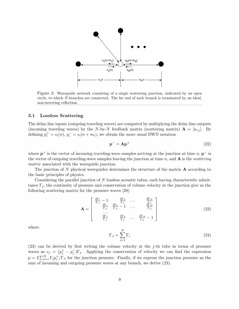
Fig. Fig. 2 illustrates an N -branch DWN which is structurally equivalent to the feedback loop ofan N -th order FDN. It consists of a single scattering junction, indicated by a white circle, to whichN branches are connected. The far end of each branch is terminated by an ideal non-invertingreflection (black circle). The waves traveling into the junction are associated with the FDN delayline outputs si(n), and the length of each waveguide is half the length of the corresponding FDNdelay line mi (since a traveling wave must traverse the branch twice to complete a round tripfrom the junction to the termination and back). When mi is odd, we may replace the reflectingtermination by a unit-sample delay.
8
s1(n+m1) sN(n+mN)
s1(n) sN(n)
m1/2 mN/2
Figure 2: Waveguide network consisting of a single scattering junction, indicated by an opencircle, to which N branches are connected. The far end of each branch is terminated by an ideal,non-inverting reflection.
3.1 Lossless Scattering
The delay-line inputs (outgoing traveling waves) are computed by multiplying the delay-line outputs(incoming traveling waves) by the N -by-N feedback matrix (scattering matrix) A = [ai,j ]. Bydefining p+
i = si(n), p−i = si(n + mi), we obtain the more usual DWN notation
p− = Ap+ (22)
where p+ is the vector of incoming traveling-wave samples arriving at the junction at time n, p− isthe vector of outgoing traveling-wave samples leaving the junction at time n, and A is the scatteringmatrix associated with the waveguide junction.
The junction of N physical waveguides determines the structure of the matrix A according tothe basic principles of physics.
Considering the parallel junction of N lossless acoustic tubes, each having characteristic admit-tance Γj , the continuity of pressure and conservation of volume velocity at the junction give us thefollowing scattering matrix for the pressure waves [28]:
A =
2Γ1
ΓJ− 1 2Γ2
ΓJ. . . 2ΓN
ΓJ2Γ1
ΓJ
2Γ2
ΓJ− 1 . . . 2ΓN
ΓJ
. . .2Γ1
ΓJ
2Γ2
ΓJ. . . 2ΓN
ΓJ− 1
(23)
where
ΓJ =N∑
i=1
Γi (24)
(23) can be derived by first writing the volume velocity at the j-th tube in terms of pressurewaves as vj = (p+
j − p−j )Γj . Applying the conservation of velocity we can find the expression
p = 2∑N
i=1 Γip+i /ΓJ for the junction pressure. Finally, if we express the junction pressure as the
sum of incoming and outgoing pressure waves at any branch, we derive (23).
9
3.2 Normalized Scattering
For ideal numerical scaling in the L2 sense, we may choose to propagate normalized waves whichlead to normalized scattering junctions analogous to those encountered in normalized ladder filters[13]. Normalized waves may be either normalized pressure p+
j = p+j
√Γi or normalized velocity
v+j = v+
j /√
Γi. Since the signal power associated with a traveling wave is simply P+| = (p+
j )2 =
(v+j )2, they may also be called root-power waves [27].
The scattering matrix for normalized pressure waves is given by
A =
2Γ1
ΓJ− 1 2
√Γ1Γ2
ΓJ. . . 2
√Γ1Γn
ΓJ
2√
Γ2Γ1
ΓJ
2Γ2
ΓJ− 1 . . . 2
√Γ2Γn
ΓJ
. . . . . .
. . . . . .2√
ΓnΓ1
ΓJ
2√
ΓnΓ2
ΓJ. . . 2Γn
ΓJ− 1
(25)
The normalized scattering matrix can be expressed as a Householder reflection
A =2
||Γ||2ΓΓT − I (26)
where ΓT = [√
Γ1, . . . ,√
ΓN ], and Γi is the wave admittance in the ith waveguide branch. Thegeometric interpretation of (26) is that the incoming pressure waves are reflected about the vectorΓ. Unnormalized scattering junctions can be expressed in the form of an “oblique” Householderreflection A = 21ΓT / 〈1,Γ〉 − I, where 1T = [1, . . . , 1] and ΓT = [Γ1, . . . , ΓN ].
3.3 Complexity
It is important to note that a Householder reflection can be implemented using O(N) numericaloperations, as opposed to O(N 2) operations for a general scattering matrix (in computing Ap+ in(26), first precompute the inner product ΓT p+ [5]). Since all junctions of N physical waveguidescan be expressed as a Householder reflection, all such scattering junctions require only O(N) com-putations.
It is interesting to note that Jot [8] proposed a class of feedback matrices for the efficientimplementation of FDNs which are specialized Householder reflections. We have just shown thatthe same kind of structure arises naturally, in the context of waveguide modeling, for physicallybased scattering matrices.
3.4 Conditions for Losslessness
The scattering matrices for lossless physical waveguide junctions give an apparently unexploredclass of lossless FDN prototypes. However, this is just a subset of all possible lossless feedbackmatrices. We are therefore interested in the most general conditions for losslessness of an FDNfeedback matrix.
Consider the general case in which A is allowed to be any scattering matrix, i.e., it is associatedwith a not-necessarily-physical junction of N physical waveguides. Following the definition of
10
losslessness in classical network theory, we may say that a waveguide scattering matrix A is said tobe lossless if the total complex power [1] at the junction is scattering invariant, i.e.,
p+∗Γp+ = p−∗
Γp−
⇒ A∗ΓA = Γ (27)
where Γ is any Hermitian, positive-definite matrix (which has an interpretation as a generalizedjunction admittance). The form x∗Γx is by definition the square of the elliptic norm of x inducedby Γ, or ||x||2
Γ= x∗Γx. Setting Γ = I, we obtain that A must be unitary. This is the case
commonly used in current FDN practice.The following theorem gives a general characterization of lossless scattering:
Theorem 1: A scattering matrix (FDN feedback matrix) A is lossless if and only if its eigenvalueslie on the unit circle and it admits a basis of linearly independent eigenvectors.Proof:In general, the Cholesky factorization Γ = U∗U gives an upper triangular matrix U which convertsA to a unitary matrix via similarity transformation: A∗ΓA = Γ⇒ A∗U∗UA = U∗U⇒ A∗A = I,where A = UAU−1. Hence, the eigenvalues of every lossless scattering matrix lie on the unit circle.It readily follows from similarity to A that A admits N linearly independent eigenvectors. In fact,A is a normal matrix (since it is unitary), and normal matrices admit a basis of linearly independenteigenvectors [21].
Conversely, assume |λ| = 1 for each eigenvalue of A, and that there exists a matrix T of lin-early independent eigenvectors of A. Then the matrix T diagonalizes A to give T−1AT = D ⇒T∗A∗T−1∗ = D∗, where D = diag(λ1, . . . , λN ). Multiplying, we obtain T∗A∗T−1∗T−1AT =D∗D = I⇒ A∗T−1∗T−1A = T−1∗T−1. Thus, (27) is satisfied for Γ = T−1∗T−1 which is Hermi-tian and positive definite. 2
Thus, lossless scattering matrices may be fully parametrized as A = T−1DT, where D isany unit-modulus diagonal matrix, and T is any invertible matrix. In the real case, we haveD = diag(±1) and T ∈ <N×N .
3.5 Relation of DWNs to FDNs
When U in the proof is diagonal and positive, a physical waveguide interpretation always existswith U = diag(Γ). A generalized waveguide interpretation exists for all U via vector transformers[28, p. 55 sec. 4] in which U acts as an ideal transformer (in the classical network theory sense) onthe vector of all N waveguide variables. If p = p+ + p− denotes the vector of physical pressuresat the junction and p = p+ + p− denotes the physical volume velocities, then we have that thejunction power, defined as PJ = p∗p is invariant with respect to insertion of a vector transformer(similarity transformation applied to the scattering matrix).
It can be quickly verified2 that all scattering matrices arising from the parallel intersectionof N physical waveguides possess one eigenvalue equal to 1 and N − 1 eigenvalues equal to −1[28]. In the case of physical waveguides of equal impedances, the eigenvector associated withthe eigenvalue 1 corresponds to equal incoming waves, while an eigenvector associated with the
2using the eigenvectors eT0 = [1, . . . , 1] and e
Tk = [1, . . . , 1, 1 − ΓJ/Γk
︸ ︷︷ ︸
kth
, 1, . . . , 1], k = 1, . . . N
11
eigenvalue −1 corresponds to equal incoming waves on N − 1 branches, and a large opposite waveon the remaining branch which pulls the junction pressure to zero. Adding a vector transformerto the parallel N -branch scattering junction gives scattering matrices of the form A = T−1DT
with D = diag(1,−1, . . . ,−1). To obtain more general eigenvalue signatures D = diag(±1), acombination of series and parallel junctions must be used. Finally, to reach the most generalcomplex case, we must admit complex eigenvalues.
We now consider the relation between unitary FDN feedback matrices and waveguide scatteringjunctions. As can be seen from comparing (27) to A∗A = I (true for any unitary matrix), we seethat A unitary corresponds to a scattering junction in which the total complex power is givenby the ordinary L2 norm of the incoming or outgoing traveling waves. Since the physical powerassociated with an incoming wave vector p+ is PJ = p+∗
Γp+, where in the absence of a vectortransformer Γ = diagΓ1, . . . , ΓN , we see that A unitary corresponds to a scattering junction joiningwaveguides of equal wave impedance, i.e., Γ = diag1, . . . , 1. Since Householder reflections compriseonly a subset unitary matrices, we see that a unitary FDN matrix corresponds to a transformer-coupled parallel/series waveguide junction in which all branch admittances are the same. Inthe more general (unnormalized) case in which the branch impedances are different, i.e., Γ =diag(Γ1, . . . , ΓN ), we obtain (using a vector transformer) the larger class of scattering matriceswhich preserve an elliptic norm as induced by a positive-definite (or Hermitian) generalized junctionimpedance.
Since, as discussed above, only a subset of all N -by-N unitary matrices is given by a physicaljunction of N waveguides, the unitary FDN point of view yields lossless systems outside the scopeof those suggested by multiport scattering theory. On the other hand, since only normalizedwaveguide junctions exhibit unitary scattering matrices, the DWN approach gives rise to newclasses of FDNs. Moreover, by considering more than one scattering junction, the DWN approachsuggests new classes of network topologies following physical analogies. Similarly, FDN matricescan be partitioned to embed several FDN subsystems into larger FDN systems.
Formally, every DWN can be expressed as an FDN by collecting all of its delay lines into adiagonal delay matrix D(z) as in (4), and finding the matrix A which computes the delay-lineinputs from the delay-line outputs. Therefore, every waveguide network yields a feedback matrixfor consideration in the FDN framework. Conversely, every real FDN can be expressed as a single-junction waveguide network using an ideal vector transformer at the junction.
Theorem 1 characterizes lossless FDN feedback matrices A as those having eigenvalues on theunit circle, where the definition of losslessness was given by (27). It remains to be shown thatA satisfying (27) implies that the poles of the corresponding FDN are all on the unit circle. Tothis end, recall the form of the state-transition matrix (8), and define the extended generalizedadmittance
Γ† =
[
I 0
0 Γ
]
(28)
By analogy to the derivation of (18), we get
A†T Γ†A† = diag(
Im1−1, . . . ImN−1,AT ΓA
)
(29)
This equation shows that A is lossless if and only if A† is lossless, and its eigenvalues are on theunit circle by Theorem 1. But from (17), we have that the eigenvalues of A† are the poles of thecorresponding FDN. Therefore, the FDN is lossless and its impulse response consists only of non-increasing and non-decaying modes. Desired decay characteristics versus frequency for obtaining a
12
specific artificial reverberator can now be controlled separately by means of attenuation coefficientsand filters, as indicated in section II.
3.6 Finite-Wordlength Effects
We have just seen how the FDN can be seen as a simple DWN having a not-necessarily physicalscattering matrix. In order to provide an easy control over the decay, the scattering matrix hasto satisfy the condition of losslessness (27). A finite-precision implementation of the FDN mightincur in limit cycles or overflow oscillations, due to departures from the infinite-precision losslessprototype. Departures can be of two kinds: the finite-precision scattering matrix does not satisfy thelossless condition (27), or the round-off noise in the matrix by vector multiplication Ap+ introducessignal amplitude modifications. By assuming that the scattering matrix satisfies (27) in a largeextent even in finite precision, it is possible to apply the arguments used in [27, 28, 26, 6] for theDWNs, in order to avoid limit cycles or overflow oscillations. If the matrix by vector multiplicationis performed in the straightforward way as a collection of inner products, and the matrix coefficientshave the same n bits of precision as the signals, it is just sufficient to perform these order-N innerproducts in the extended precision of 2n+N−1 bits, and apply a passive truncation scheme on theoutput signal. In two’s complement arithmetic, a simple passive truncation scheme is the following:
• If the N-1 most significant bits are not equal, replace the output value by the maximum-magnitude number in n-bit two’s complement having the correct sign (saturation).
• Discard the n least significant bits and add 2−n+1 to the result if it is negative.
As far as the condition on the losslessness of the scattering matrix is concerned, general requirementsfor the construction of “structurally lossless,” or at least “structurally passive” scattering matriceshave to be worked out. This topic, previously touched by Gray [6] in the N = 2 case, will bediscussed in a forthcoming paper, since a complete treatment would enlarge the scope of this papersignificantly.
4 Circulant Feedback Delay Networks
Consider the class of circulant feedback matrices having the form
This class of matrices gives rise to a class of FDNs we call Circulant Feedback Delay Networks(CFDN). The following two facts can be proved [3]:
Fact 1 : If a matrix is circulant, it is normal, i.e., A∗A = AA∗.
Fact 2 : If a matrix is circulant and lossless, it is unitary.
13
It is well known that every circulant matrix is diagonalized by the Discrete Fourier Transform(DFT) matrix [3]. This implies that the eigenvalues of A can be computed by means of the DFTof the first row:
λ(A) = A(k) = DFT ([a(0) . . . a(N − 1)]T )
where λ(A) denotes the set of all eigenvalues of A, and A(k) denotes the set of complex DFTsamples obtained from taking the DFT of a(·).
4.1 Design of Poles and Zeros in CFDNs
A matrix that is both unitary and circulant has all eigenvalues on the unit circle, and the DFT canbe used to compute the eigenvalue phases. In the case of equal-length delay lines, the eigenvaluesdetermine the resonance frequencies in a simple way. From (16), when D(z−1) = zmI, the systempoles are the m-th complex roots of the eigenvalues of A.
Conversely, we can easily design a circulant matrix to have a desired distribution of eigenvalues.This is also true for any lossless matrix, since Theorem 1 gives that any A of the form A = T−1DT
is lossless, where D is any unit-modulus diagonal matrix, and T is any invertible matrix. Thus, alossless matrix is characterized by the arguments of its eigenvalues and a similarity transformationmatrix T. The advantage of choosing circulant FDNs over other kinds of FDNs is the possibilityof computing A from its eigenvalues very efficiently by means of a single inverse FFT.
As we will see in section V, in a practical implementation the delay lengths are typically notequal. However, the equal-delay case is easier to analyze. The limitations and advantages of sucha choice will become clearer in section V.
The actual presence of resonance peaks corresponding to the eigenvalues depends on the posi-tions of the zeros, as given by (19). Assuming equal-length delay lines and d = 1, (19) becomes
det[A− bcT − zmI] = 0 (30)
which means that the zeros are the m-th complex roots of the eigenvalues of A− bcT .In order to have “colorless” reverberation, it may be desirable to make the envelope of the
amplitude response flat. To do this, each zero should be equal to the reciprocal of a pole. Inprototype CFDNs, the feedback matrix is lossless, and the system poles are on the unit circle, sothe zeros must equal the poles. However, when all zeros and poles cancel exactly, the impulseresponse of the FDN degenerates to an impulse.3 This is a general problem with any all-passreverberator: Lengthening the reverberation time without changing the delay lengths forces theimpulse response converge to an impulse. In our case, we depart from the idealized case by slightlychanging the delay lengths. As we will show in section V, this approach leads to reverberatorshaving a frequency response which is nearly flat at low frequencies, while preserving the richnessof the echo density in the time domain.
Therefore, we continue treating the prototype case of equal-length delay lines and d = 1, andshow that we can obtain perfect canceling of zeros and poles by using (1) bT = [1, 1, . . . , 1] and(2) c having n entries equal to 1, n entries equal to −1, and zeros for the remaining entries. Thisresult is due to the following
3Since we are discussing discrete-time systems, the term “impulse” means the same thing as “unit sample pulse.”
14
Theorem 2: Given a circulant NxN matrix A, let A′ be obtained by adding a constant c toeach entry of n rows (columns) and subtracting the same constant c from each entry of another nrows (columns). Then A and A′ have the same eigenvalues.
Before providing the proof of Theorem 2, we need to prove the followingLemma: All the eigenvectors of a circulant matrix other than the “dc” vector [1, . . . , 1]T lie
in the null space of any matrix with constant rows. Thus, adding constant rows cannot altereigenvalues or eigenvectors other than the 0th.
Proof: This follows immediately from the fact that the eigenvectors of every circulant matrixare given by the columns of the DFT matrix of the same size, and these vectors are orthogo-nal. Therefore, a constant row is orthogonal to all eigenvectors of the DFT matrix except the dceigenvector.
The lemma states that all we can do by adding constant rows to a circulant matrix is move the“dc” eigenvector to some other vector and change its eigenvalue.
Proof of Theorem 2:Consider the matrix A′ given by:
A′ = A− bcT (31)
where bT = [1,−1, 0, . . . , 0] and cT = [1, 1, . . . , 1]. Since any circulant matrix is diagonalized bythe DFT matrix, if we pre-multiply and post-multiply both sides of (31) by the DFT matrices F∗
and F, we obtainF∗A′F = F∗AF− F∗bcTF = D− F∗(bcTF)
where D is a diagonal matrix and the term within parentheses is an N by N matrix having non-nullentries only in position (1,1) and (2,1). Moreover these two entries have opposite sign. It turnsout that F∗bcTF has non-null elements only on the first column under the diagonal. This meansthat the matrix A′ can be triangularized by means of the DFT matrix and its eigenvalues (foundon the diagonal) are the same as those of A. This argument works for any number of oppositelysigned couples of distinct values arbitrarily distributed in the vector b. The same argument can befollowed for proving the claim relative to the columns. In this case we would start by forming theproduct F∗bcT . 2
Note that the 0th eigenvalue is no longer a “dc” eigenvalue. The corresponding eigenvectormust be found in ker(A−bcT − λ0I), where ker() gives the nullspace of its argument. In the caseof a real circulant matrix A with eigenvalues along the unit circle, we have that λ0 = 1 (the sumof the elements of a row of A is 1).
With the above choice of b and c coefficients, we obtain a perfectly flat amplitude responsefor equal-length delay lines. However, this is degenerate since this is the condition for pole-zerocancellation. As we will show in section V, when using slightly different delay lengths, a nearly flatresponse at low frequencies is obtained as a perturbation of the pole-zero cancellation configuration.
4.2 Computational Complexity
In an N -th order FDN, the core computations consist of N updates of the delay lines and a matrixby vector multiplication. The delay line operations can proceed in parallel. The matrix by vectormultiplication requires in general O(N 2) operations (multiplications and additions). If the matricesarise from the scattering coefficients of a waveguide junction, the computations reduce to O(N).The same order of complexity is required by the normalized waveguide junction. For the special
15
case of a junction of equal-impedance waveguides, the multiplications can be replaced by shiftswhen N is a power of 2 [26]. In all these efficient cases the eigenvalues of the feedback matrix areconstrained to be at +1 or -1. The circulant matrix offers a more general eigenvalue distribution.Moreover, the matrix by vector multiplication can be implemented very efficiently in hardware.This multiplication can be viewed as a circular convolution of the column vector with the firstrow of the matrix. Such a convolution can be performed, when N is a power of 2, using twoFFTs (one of which can be precomputed), an elementwise product between two N -vectors, andan inverse FFT. The complexity of this algorithm is O(N log(N)). It is easy to implement thismatrix-vector product in VLSI by means of the butterfly or other hypercubic architectures [12].These architectures allow computations of the FFT in O(log(N)) time steps, and the algorithmcan be pipelined.
The parallel implementation of waveguide scattering matrices cannot be done in less thanO(log(N)) time steps, because of the scalar product that is involved in Householder reflectionsof any kind. Hence, in parallel implementations we lose the advantage of waveguide scatteringmatrices over circulant matrices.
Moreover, we can use number-theoretic Fourier transforms [12] in order to compute the circularconvolution. Such transforms work over commutative rings, and can be arranged in such a waythat all multiplications are replaced by shifts. Since in the convolution we have both the direct andinverse transforms, the overall result remains correct.
The circulant structure of A is advantageous for purposes of real-time control as well. In thefirst place, the entire matrix is determined by one of its rows or columns, and no matter how arow or column is modified, as long as the rest of the matrix is modified accordingly to preservethe circulant structure, the matrix will have unit-modulus eigenvalues as needed for losslessness.Furthermore, the top row of a circulant matrix is obtained from its eigenvalues by means of aninverse DFT. Therefore, it is possible to efficiently generate a continuous family of circulant matricesby continuously varying the complex phases of the eigenvalues. Moreover, if the matrix-vectormultiplication is implemented in the frequency domain, the inverse DFT is not needed. Thus, wemay move the N eigenvalues to arbitrary points on the unit circle and generate a wide family ofefficiently computed lossless feedback matrices.
5 Applications
We have been using circulant networks for various purposes in sound synthesis and processing.Artificial reverberation is probably the most significant application, but other significant areas ofinterest can be found in sound synthesis and filtering.
5.1 Digital Reverberation
Two quantities have been proposed as criteria for measuring the “naturalness” of synthetic rever-beration: the time density and the frequency density [8]. A good reverberator should provide highvalues of both densities, thus giving smooth, dense time and frequency responses.
The frequency density Df is defined as the average number of resonances per Hertz. A generalexpression can be derived from the order of the system (5), assuming that all the poles are distinct
16
and no cancellation occurs:
Df =1
Fs
N∑
i=1
mi (32)
In real rooms, the frequency density increases at higher frequencies (as can be seen from (35)below).
In the prototype case where the delay lines all have the same length m, we have
Df =Nm
Fs
(33)
The time density Dt is defined as the number of nonzero samples per second in the impulse re-sponse. In actual rooms, Dt is an increasing function of time. In order to obtain dense reverberationafter the early reflections (e.g., after 80 msec), it helps to use different delay lengths.
The actual positions of frequency peaks depend on the feedback matrix and the delay lengths.If the delay lengths are fixed, we can vary some time-frequency properties of the structure simplyby varying the distribution of eigenvalues of the feedback matrix. The total length of the delaylines should be chosen in such a way that the frequency density, as determined by (32), is highenough. Then the matrix eigenvalues can be adjusted to avoid resonant peak clustering or otherundesirable mode distributions.
It is interesting to discuss the effect of eigenvalues in the prototype case of equal delays. Auniform distribution of eigenvalues along the unit circle is optimum for the frequency response inthe sense that it minimizes the maximum distance between peaks. However, it produces a highlyrepetitive time response. Conversely, clustering the eigenvalues around a point on the unit circlecan be good for maximizing the length of time patterns, but the clustering of frequency peaksproduces a poor reverberator amplitude response vs. frequency. We see from these considerationsthat there is a time-frequency tradeoff. This tradeoff can be addressed using circulant matrices.
A couple of examples of different eigenvalue distributions are given in Fig. Fig. 3. The matrix A2
used in Fig. Fig. 3b is simply obtained by a right circular shift of the rows of the matrix A1 whichis given by the junction of equal-impedance waveguides and, as already stated, has eigenvalues onlyat 1 and −1. We can express A2 as the product A1Π where Π is the right-shift matrix
Π =
0 1 00 0 11 0 0
. (34)
Both A1 and Π are circulant, therefore the eigenvalues of A2 are given by the collection of theelement-wise products of the eigenvalues of A1 and the eigenvalues of Π, which are the N -thcomplex roots of 1 [3]. For clarity, we set all the delay lengths equal in the examples.
As a side comment, we notice that Π is the scattering matrix of the circulator, a circuit devicewhich can be used to obtain the multiplication of one-port scattering parameters [18].
The shape of the frequency response depends also on the zeros which were discussed in sectionIV. In particular, Theorem 2 provides a way of setting the zeros exactly over the poles in theprototype equal-delay case. We anticipated in section IV that the way to choose the vectors b andc indicated in Theorem 2 can be useful for getting a flat amplitude response at low frequencieswhen the delay lengths are slightly varied from the prototype case. Fig. Fig. 4 depicts the timeand frequency responses for the CFDN using the same feedback matrix as in Fig. Fig. 3b, having
17
a)
0 500 1000 1500 2000Samples
Impulse Response
0.001
0.01
0.1
1
10.
2153 4306Hz
Frequency Response
-20
-10
0dB
b)
0 500 1000 1500 2000Samples
Impulse Response
0.001
0.01
0.1
1
10.
0 500 1000 1500 2000Samples
Impulse Response
0.001
0.01
0.1
1
10.
2153 4306Hz
Frequency Response
-20
-10
0dB
A1 =
−1/3 2/3 2/32/3 −1/3 2/32/3 2/3 −1/3
A2 =
2/3 −1/3 2/32/3 2/3 −1/3−1/3 2/3 2/3
λ1 =[−1 1 −1
]λ2 =
[e−jπ/3 1 ejπ/3
]
Figure 3: Time and Frequency behaviors for two Circulant Feedback Delay Networks which differonly by a shift on the rows of the feedback matrix.
18
a)
0 500 1000 1500 2000Samples
Impulse Response
0.001
0.01
0.1
1
10.
b)
2153 4306Hz
Frequency Response
-20
-10
0
dB
Figure 4: Zero positioning which gives a nearly flat low-frequency response for the CFDN of Fig.3b.
19
bT = [1, 1, 1], cT = [0,−1, 1], and delay lengths m = [16, 17, 15]. As we can see from Fig. Fig. 4, weare able to get a nearly flat amplitude response at low frequencies without losing the reverberatingcharacter of the time response. We believe that this is a good alternative to allpass filters whichtend to have degenerate impulse responses when the poles approach the unit circle.
5.2 Physical Room Modeling with FDNs
A flat amplitude response at low frequencies, while desirable in several practical situations, is notfound in actual rooms. Therefore, if the goal is to model the reverberation of a physical room,the way indicated by Theorem 2 is not appropriate. Somewhat happily, the FDN can be thekernel of a model of rectangular room, and its parameters can be interpreted in a physical andgeometrical framework. In this section, we give only a sketch of this framework, since the detailsof the underlying metaphor are beyond the scope of this paper, and can be found in [23].
Consider a lossless shoe-box shaped room, having length lx, depth ly, and height lz. For such aroom, it is possible to compute analytically the frequencies of the normal modes [17] as
fnx,ny ,nz =c
2
√√√√√
(nx
lx
)2
+
(
ny
ly
)2
+
(nz
lz
)2
(35)
where nx, ny, nz = 0, 1, 2, . . ., and c is the speed of sound in air. Each normal mode is associatedwith a direction in space, whose cosines, made by the wave propagation with respect to the x, y,and z axes, are
vx
v=
nxc
2flx,
vy
v=
nyc
2fly,
vz
v=
nzc
2flz, (36)
where v is the magnitude of the (vector) spatial frequency, and the subscripts in fnx,ny ,nz havebeen dropped for conciseness.
The triple n = (nx, ny, nz) completely characterizes a normal mode. All the triples which aremultiples are associated with a harmonic series of frequencies and with the same direction in space.This suggests that any harmonic series of normal mode frequencies can be obtained by means ofa linear resonator (in other words, a comb filter) whose length in seconds is set to d0 = 1/f0,where f0 is the fundamental frequency of the harmonic series. Therefore, we can decompose themodal distribution of the response of an actual room into harmonic subsets (a harmonic of fnx,ny ,nz
is obtained by multiplying nx, ny, and nz by the same integer). Sorting these harmonic subsetsaccording to their fundamental frequencies and taking the reciprocals of the N lowest fundamentalfrequencies yields a parallel comb filter representation of the room (i.e., an FDN with diagonalfeedback matrix), so that the FDN reproduces the lowest eigenfrequencies exactly. This procedurewas already outlined in [8] as a mean of identifying the parallel comb-filter parameters from ameasured impulse response.
We can elaborate the representation further by interpreting the quantity d0 as the time takenby a plane wavefront to travel a certain distance along the direction (36) in space. In fact, a normalmode and all its harmonically related multiples can be thought of as a plane wave bouncing backand forth in the closed environment [17]. For a finite medium, in order to support such an infiniteplane wave, the planar fronts have to be bent at the walls such that they form a constant-area closedsurface. It can be verified that the time d0 is the time interval between two successive collision ofplane wavefronts.
20
Once established that, in an idealized rectangular room, each harmonic subset of normal modescan be represented by a linear resonator oriented along a given direction in space, we can introduceother “second-order” effects into the basic model.
Let us consider an octant in space. Taking the first N fundamental frequencies in the harmonic-subset decomposition of the normal modes corresponds to sampling in space along N directions.An object in any point of the space will provide scattering among the N directions. The wallsthemselves, when they are not ideally smooth, scatter the waves among different directions. Wecan think of lumping all these diffusion effects and representing them in the non-diagonal elementsof the scattering matrix of a FDN. With some approximation, it was also shown in [23] thatan isotropic object in a non-diffusive rectangular room can be represented by a circulant matrix,provided that the spatial sampling is almost uniform and the proper ordering of directions is chosen.
The geometric interpretation allows one to properly excite the modes according to the positionof the sound source, by just replacing each coefficient in the vector b by a suitable cascade ofFIR comb filters [23]. The position where we listen to the sound is related to the c coefficients ina similar way. It is also quite easy to take into account the radiation pattern of the source andthe directivity of the pick-up. Perhaps more importantly, the absorption coefficients of the wallscan be made direction-dependent, as they are found in reality, as they affect the different “linearresonators” differently.
In the model at hand, the matrix element ai,j scales the signal transmission from mode j tomode i. The diagonal of the feedback matrix determines the strength of the “standing waves” setup along each pattern. Equivalently, we can think of a DWN modeling the parallel junction of Nacoustic tubes, where each tube gives rise to a harmonic subset of normal modes.
The physical modeling viewpoint is limited by the fact that only N “standing-wave paths” inthe room are being simulated, and all non-specular reflections are being forced to enter some subsetof the supported ray paths.
In the model, the diffusivity of the whole reverb is lumped in the properties of the scatteringmatrix. This is a dramatic simplification, but it allows better control of diffusivity in isolation fromother room parameters.
The geometrical interpretation is useful for computing the lengths of the delay lines accordingto the dimensions of a particular room, since each wavefront path corresponds to a normal mode. Inprevious work on artificial reverberation [25, 16], the choice of the delay-line lengths in the all-passand comb-filter sections is a primary issue. Typically, the choice is guided by heuristic rules ornumber-theoretic criteria, and a lot of trial and error is often necessary to obtain good values.
5.3 Physical Room Modeling with DWNs
Recent developments in physical modeling using digital waveguides have included the use of awaveguide mesh to model 2D membranes and 3D rooms [32, 33, 24]. In the membrane, for example,a rectilinear mesh of digital waveguides can be interconnected via four-port scattering junctions toprovide lossless prototypes for “plate reverberators” and the like. A single dispersive waveguide(made dispersive using embedded allpass filters) can be used to model “spring reverberators.”Savioja et al. [24] have found that the rectilinear 3D waveguide mesh has good room simulationproperties at low frequencies.
Since reverberation quality generally increases with the number dimensions (from spring toplate to acoustic space), it is plausible to expect that higher dimensional waveguide meshes willprovide better reverberation than we have ever known. Generalizing (35) to higher dimensions,
21
one can see that the higher the dimensionality, the more rapidly the mode density increases withfrequency. However, above the “Schroeder limit” at which the modes are so densely packed thatthe ear cannot resolve them, increasing the density should have no audible effect. Nevertheless, itis an interesting direction to pursue.
The waveguide mesh is structurally lossless so that there is no attenuation error in the sampledwave propagation. However, the grid quantization does give rise to dispersion error: The speedof sound effectively varies somewhat as a function of frequency and propagation direction on themesh. Generally, results are very accurate at low frequencies, but sound speed decreases graduallyas frequency increases in all but certain directions which tend to be diagonals along the mesh [32].The choice of mesh geometry has a strong effect on the dispersion behavior [33]. It also stronglyaffects computational complexity. As an example, whenever an isotropic mesh utilizes N -portscattering junctions in which N is a power of 2, the scattering matrices require no multiplies [26].For rectilinear meshes, membranes are multiply free, as are solids in 4D (since the number of portsis 2N , in N dimensional space). The tetrahedral mesh, analogous to the diamond crystal, requiresno multiplies to fill 3D space. Multiply-free waveguide meshes can be integrated very densely inVLSI.
A final word about waveguide meshes is that they, like any other LTI system, can be expressedin a sparse state-space form which yields an FDN that can be interpreted as a physical model.
5.4 Practical FDN Design
In our experience, given an FDN reverberator structure, setting the delay lengths can be a rathertedious job. The vast majority of possible delays just provide poor results in the sense that thetime response is too “rough” or the frequency response is too “colored.” An interesting approachto this problem might be to use nonlinear optimization techniques such as “simulated annealing”or “genetic algorithms” to optimize the delay lengths such that “perceptual uniformity” of theresponse is maximized in the time and frequency domains jointly.
Designing the delay lengths from room geometry has the property of giving a reverberatorwhich is always consistent with a desired room in that the low-frequency modes are matched.However, there does not seem to be any compelling reason to match specific low-frequency modetunings. Noticeable room resonances are normally perceived as defects in a listening space. Earlyreflections, on the other hand, contribute strongly to the perceived “spatial impression” [2]. In otherapplications, however, such as modeling the soundboard of a piano as a reverberator, the specificcoloring or “equalization” provided by the reverberator is important and must be preserved. Insuch applications, it is normally necessary to match low-frequency resonances accurately and high-frequency resonances only statistically.
When the FDN order is large (larger than 8 for satisfactory results), poor results can still beobtained when modeling desired room dimensions which are not favorable. In fact, even for the shoe-box room shape, the relative dimensions play a very important role in determining the smoothnessof the reverb [15]. Of course, diffusion contributes significant smoothing to the response, so fullfeedback matrices (as opposed to diagonal feedback matrices) are especially needed to achieve goodreverberators using low-order FDNs.
On balance, it seems that what is needed for good reverberator design in general is
(1) precise matching of early reflections,
(2) minimal coloration due to uneven mode distributions in the frequency domain,
22
(3) an appropriate smoothly declining decay-time versus frequency, and
(4) smooth, rich echo density late in the impulse response, having no noticeable patterns.
These desiderata indicate that, rather than attempting to model real rooms, lossless prototypeFDNs optimizing criteria (2) and (4) should be found, for a given order, which have at least onedelay line long enough to support injection of specific early reflections to satisfy (1), and thenlowpass filters as in (21) should be added to satisty criterion (3). The main open issue is how theoptimization of (2) and (4) should best be carried out for specific classes of structurally losslessfeedback matrices.
5.5 Resonators
FDN’s with short delay lines may be used to produce resonances irregularly spread over frequency.A possible application could be the simulation of resonances in the body or soundboard of a stringinstrument.
M. Mathews and J. Kohut [14] showed that, in this kind of simulation of the violin body, theexact position and height of resonances is not usually important; on the contrary, they stated thatthe Q’s of the resonances must be sufficiently large and the peaks must be sufficiently close together.Thus, even in rather small physical resonators, a statistical matching may be as effective as a moreprecise, mode-for-mode matching.
With CFDNs we can easily achieve these goals, and we can vary the distribution of peaks byacting on the delay lengths and/or the feedback matrix. In this context, the main advantage ofusing CFDNs over general FDNs is that the feedback matrix has N parameters which are relatedto the eigenvalues by means of a DFT. This means we have the possibility of controlling a largenumber of resonances using a number of parameters which is linear in the order of the structure,and the parameter control can be performed very efficiently and safely, i.e., without running intoinstabilities. The control over matrix eigenvalues is complementary with respect to the control ofdelay lengths: while changing a delay has a stretching or squeezing effect on resonance positions allalong the frequency axis, changing the eigenvalues produces alternative changes in the distributionof resonances, such as clustering the peaks, as is illustrated in Fig. Fig. 3.
Another interesting application of CFDNs is as resonators in a feedback loop for pseudo-physicalsound-synthesis techniques. By exciting these structures with bursts of white noise we obtain amultidimensional extension of the Karplus-Strong algorithm [11], that is very effective for simulatingmembranes and bars. Alternatively, we can couple these resonators with nonlinear exciters andexplore new families of sustained sounds as in waveguide synthesis [29].
We have been using effectively CFDNs in live-electronic performances, where the exciting signalis coming from a traditional instrument, and the CFDN provides a complicated filtering patternwhose frequency shape can be controlled in real-time by its parameters (eigenvalues or row ele-ments).
6 Conclusion
This paper presented generalizations and new special cases for the matrix used in Feedback DelayNetworks. In particular, necessary and sufficient conditions were derived for losslessness of such amatrix. The correspondence between FDNs and Digital Waveguide Networks can be used to obtain
23
FDN parameters based on the physics and geometry of a real acoustic space, rather than by rulesof thumb or number-theoretic rules.
In proposing the CFDN structure, we have tried to achieve two goals: efficiency and versatilitywith respect to the time-frequency behavior. Efficiency is achieved by taking advantage of thecirculant structure of the feedback matrix, and it increases with the size of the matrix. Versatilityis achieved by introducing the matrix eigenvalues into the design process for artificial reverberators.Passing from the eigenvalues to the matrix coefficients requires only a single inverse DFT or FFT.Eigenvalues act on the distribution of frequency peaks, thus giving controls pertaining to the colorand smoothness of the reverberation.
In addition to application of CFDNs in artificial reverberation, we have outlined some otheruses as resonators in sound synthesis and processing.
24
Index
Circulant Feedback Delay Networks, 13
elliptic norm, 11
lossless, 11
25
References
[1] V. Belevitch, Classical Network Theory, San Francisco: Holden Day, 1968.
[2] J. Borish, Electronic Simulation of Auditorium Acoustics, PhD thesis, Elec. Engineer-ing Dept., Stanford University (CCRMA), 1984, CCRMA Technical Report STAN-M-18,http://ccrma.stanford.edu/STANM/stanm18/.
[3] P. J. Davis, Circulant Matrices, New York: John Wiley and Sons, Inc., 1979.
[4] M. A. Gerzon, “Unitary (energy preserving) multichannel networks with feedbacks,” Electron-ics Letters, vol. 12, no. 11, pp. 278–279, 1976.
[5] G. H. Golub and C. F. Van Loan, Matrix Computations, 2nd Edition, Baltimore: The JohnsHopkins University Press, 1989.
[6] A. H. Gray, “Passive cascaded lattice digital filters,” IEEE Transactions on Acoustics, Speech,Signal Processing, vol. ASSP-27, pp. 337–344, May 1980.
[7] D. A. Jaffe and J. O. Smith, “Extensions of the Karplus-Strong plucked string algorithm,”Computer Music Journal, vol. 7, no. 2, pp. 56–69, 1983, Reprinted in [22].
[8] J.-M. Jot, Etude et Realization d’un Spatialisatuer de Sons par Modeles Physiques et Perceptifs,PhD thesis, French Telecom, Paris, Paris 92 E 019, 1992, written in French.
[9] J.-M. Jot and A. Chaigne, “Digital delay networks for designing artificial reverberators,” AudioEngineering Society Convention, Feb. 1991.
[10] T. Kailath, Linear Systems, Englewood Cliffs, NJ: Prentice-Hall, Inc., 1980.
[11] K. Karplus and A. Strong, “Digital synthesis of plucked string and drum timbres,” ComputerMusic Journal, vol. 7, no. 2, pp. 43–55, 1983.
[12] F. T. Leighton, Introduction to Parallel Algorithms and Architectures : Arrays, Trees, Hyper-cubes, Los Altos, California: William Kaufmann, Inc., 1992.
[13] J. D. Markel and A. H. Gray, Linear Prediction of Speech, New York: Springer Verlag, 1976.
[14] M. Mathews and J. Kohut, “Electronic simulation of violin resonances,” Journal of the Acous-tical Society of America, vol. 53, no. 6, pp. 1620–1626, 1973.
[15] J. Milner and R. Bernhard, “An investigation of the modal characteristics of nonrectangularreverberation rooms,” Journal of the Acoustical Society of America, vol. 85, no. 2, pp. 772–779,1989.
[16] J. A. Moorer, “About this reverberation business,” Computer Music Journal, vol. 3, no. 2,pp. 13–18, 1979, reprinted in [?].
[17] P. M. Morse, Vibration and Sound, http://asa.aip.org/publications.html: AmericanInstitute of Physics, for the Acoustical Society of America, 1948, 1st edition 1936, last author’sedition 1948, ASA edition 1981.
[18] R. W. Newcomb, Linear Multiport Synthesis, New York: McGraw-Hill, 1966.
[19] A. V. Oppenheim and R. W. Schafer, Digital Signal Processing, Englewood Cliffs, NJ: Prentice-Hall, Inc., 1975.
[20] J. M. Ortega, Numerical Analysis, New York: Academic Press, 1972.
[21] S. Perlis, Theory of Matrices, New York: Dover, 1991, 1st ed. 1952.
[22] C. Roads, ed., The Music Machine, Cambridge, MA: MIT Press, 1989.
[23] D. Rocchesso, “The ball within the box: A sound-processing metaphor,” Computer MusicJournal, vol. 19, Winter 1995.
[24] L. Savioja, J. Backman, A. Jarvinen, and T. Takala, “Waveguide mesh method for low-frequency simulation of room acoustics,” Proceedings of the 15th International Conferenceon Acoustics (ICA-95), Trondheim, Norway, pp. 637–640, June 1995.
[25] M. R. Schroeder, “Natural-sounding artificial reverberation,” Journal of the Audio EngineeringSociety, vol. 10, no. 3, pp. 219–233, 1962.
[26] J. O. Smith, “A new approach to digital reverberation using closed waveguide networks,”in Proceedings of the 1985 International Computer Music Conference, Vancouver, pp. 47–53,Computer Music Association, 1985, also available in [28].
[27] J. O. Smith, “Elimination of limit cycles and overflow oscillations in time-varying lattice andladder digital filters,” in Proceedings of the IEEE Conference on Circuits and Systems, SanJose, pp. 197–299, May 1986, conference version; full version available in [28].
[28] J. O. Smith, “Music applications of digital waveguides,” Tech. Rep. STAN–M–39, CCRMA,Music Department, Stanford University, 1987, a compendium containing four related pa-pers and presentation overheads on digital waveguide reverberation, synthesis, and filtering,CCRMA Technical Report STAN-M-39, http://ccrma.stanford.edu/STANM/stanm39/.
[29] J. O. Smith, “Physical modeling using digital waveguides,” Computer Music Journal, vol. 16,pp. 74–91, Winter 1992, special issue: Physical Modeling of Musical Instruments, Part I.Available online at http://ccrma.stanford.edu/~jos/pmudw/.
[30] J. Stautner and M. Puckette, “Designing multichannel reverberators,” Computer Music Jour-nal, vol. 6, pp. 52–65, Spring 1982.
[31] P. P. Vaidyanathan, Multirate Systems and Filter Banks, Englewood Cliffs, NJ: Prentice-Hall,Inc., 1993.
[32] S. A. Van Duyne and J. O. Smith, “Physical modeling with the 2-D digitalwaveguide mesh,” in Proceedings of the 1993 International Computer Music Confer-ence, Tokyo, pp. 40–47, Computer Music Association, 1993, available online athttp://ccrma.stanford.edu/~jos/pdf/mesh.pdf.
[33] S. A. Van Duyne and J. O. Smith, “The tetrahedral waveguide mesh: Multiply-free computa-tion of wave propagation in free space,” in Proceedings of the IEEE Workshop on Applicationsof Signal Processing to Audio and Acoustics, New Paltz, NY, (New York), pp. 9a.6.1–4, IEEEPress, Oct. 1995.
Davide Rocchesso is a PhD candidate at the Dipartimento di Elettronica e Informatica,Universita di Padova - Italy. He received his Electrical Engineering degree from the Universitadi Padova in 1992, with a dissertation on real-time physical modeling of music instruments. In1994 and 1995, he was visiting scholar at the Center for Computer Research in Music and Acous-tics (CCRMA), Stanford University. He has been collaborating with the Centro di SonologiaComputazionale (CSC) dell’Universita di Padova since 1991, as a researcher and a live-electronicdesigner/performer. His main interests are in audio signal processing, physical modeling, soundreverberation and spatialization, parallel algorithms. Since 1995 he has been a member of theBoard of Directors of the Associazione di Informatica Musicale Italiana (AIMI).
Julius O. Smith received the B.S.E.E. degree from Rice University, Houston, TX, in 1975.He received the M.S. and Ph.D. degrees from Stanford University, Stanford, CA, in 1978 and 1983,respectively. His Ph.D. research involved the application of digital signal processing and systemidentification techniques to the modeling and synthesis of the violin, clarinet, reverberant spaces,and other musical systems. From 1975 to 1977 he worked in the Signal Processing Department atESL, Synnyvale, CA, on systems for digital communications. From 1982 to 1986 he was with theAdaptive Systems Department at Systems Control Technology, Palo Alto, CA, where he workedin the areas of adaptive filtering and spectral estimation. From 1986 to 1991 he was employed atNeXT Computer, Inc., responsible for sound, music, and signal processing software for the NeXTworkstation. Since then he has been an Associate Professor at the Center for Computer Researchin Music and Acoustics (CCRMA) at Stanford teaching courses in signal processing and musictechnology, and pursuing research in signal processing techniques applied to music and audio.


![Elliptic genera and elliptic cohomology - Long Island Universitymyweb.liu.edu/~dredden/EllipticGenera.pdf · the history of elliptic genera and elliptic cohomology, [Seg] explains](https://static.documents.pub/doc/80x56/5edc8698ad6a402d66673899/elliptic-genera-and-elliptic-cohomology-long-island-dreddenellipticgenerapdf.jpg)


