257
Classical Differential Geometry Peter Petersen

Classical Differential Geometry
Peter Petersen


Preface
This is an evolving set of lecture notes on the classical theory of curves andsurfaces. More pictures will be added eventually. I recommend people download3DXplorMath to check out the constructions of curves and surfaces with this app.It can also be used to create new curves and surfaces in parametric form. Otheruseful and free apps are Geogebra, Grapher (on Mac), and WolframAlpha.
At a minimum, a one quarter course should cover chapter 1, sections 2.1, 3.1,3.2, and chapters 4, 5. In a semester course it’d be possible to cover more fromchapter 2 and also delve into chapter 6. Chapters 6 and 7 can be covered in asecond quarter class. Note that section 2.2 is a necessary prerequisite for provingthe general Gauss-Bonnet in section 6.5.
An excellent reference for the classical treatment of differential geometry is thebook by Struik [3]. The more descriptive guide by Hilbert and Cohn-Vossen [1] isalso highly recommended. This book covers both geometry and differential geome-try essentially without the use of calculus, offers many interesting results, and givesexcellent descriptions of many of the constructions and results in differential geom-etry. Finally, after having completed these notes, I realized that Hopf’s lectures in[2] is a superb treatment of the global theory of curves and surfaces.
This text is fairly classical and is not intended as an introduction to abstract2-dimensional Riemannian geometry. In fact, in a break with the modern traditionof how to present the subject, we do not discuss covariant differentiation or paralleltranslation. Most proofs are local in nature and try to use only basic linear algebraand multivariable calculus. The only sense in which the text is more modern isin not using the language of differentials and infinitesimals as most of the classicaltexts do.
Note: Differentiability assumptions are not specific, but “as needed” for theproof to work. Basic results from analysis and linear algebra, such as implicit andinverse function theorems etc, are used freely without further justification.
Some standard topics are not covered in the text. However, I hope most ofthem can be found among the exercises. As such, they can easily be incorporatedinto lectures as the instructor sees fit.
I’d like to thank Chadwick Sprouse and Michael Williams for trying out thesenotes and providing valuable feedback.
“Reading your notes is like reading poetry, and I don’t under-stand that either.” Reed Douglas, UCLA student.
i

Contents
Preface i
Chapter 1. General Curve Theory 11.1. Curves 1Exercises 101.2. Arclength and Linear Motion 14Exercises 191.3. Curvature 22Exercises 271.4. Integral Curves 30Exercises 35
Chapter 2. Planar Curves 382.1. The Fundamental Equations 38Exercises 412.2. The Rotation Index 45Exercises 492.3. Three Interesting Results 51Exercises 562.4. Convex Curves 57Exercises 59
Chapter 3. Space Curves 623.1. The Fundamental Equations 62Exercises 673.2. Characterizations of Space Curves 70Exercises 723.3. Closed Space Curves 75Exercises 78
Chapter 4. Basic Surface Theory 804.1. Surfaces 80Exercises 834.2. Tangent Spaces and Maps 86Exercises 914.3. The First Fundamental Form 93Exercises 974.4. Special Maps and Parametrizations 100Exercises 104
Chapter 5. Curvature of Surfaces 109
ii

CONTENTS iii
5.1. Curves on Surfaces 109Exercises 1145.2. The Gauss and Weingarten Maps and Equations 116Exercises 1225.3. The Gauss and Mean Curvatures 125Exercises 1325.4. Principal Curvatures 139Exercises 1425.5. Ruled Surfaces 145Exercises 152
Chapter 6. Surface Theory 1576.1. Generalized and Abstract Surfaces 157Exercises 1626.2. Curvature on Abstract Surfaces 163Exercises 1676.3. The Gauss and Codazzi Equations 169Exercises 1786.4. The Gauss-Bonnet Theorem 182Exercises 1866.5. Topology of Surfaces 187Exercises 1906.6. Closed and Convex Surfaces 191Exercises 193
Chapter 7. Geodesics and Metric Geometry 1957.1. Geodesics 195Exercises 2007.2. Mixed Partials 202Exercises 2057.3. Shortest Curves 206Exercises 2097.4. Short Geodesics 2097.5. Distance and Completeness 213Exercises 2157.6. Isometries 215Exercises 2187.7. Constant Curvature 2197.8. Comparison Results 221
Chapter 8. Riemannian Geometry 225
Appendix A. Vector Calculus 230A.1. Vector and Matrix Notation 230A.2. Geometry 232A.3. Geometry of Space-Time 233A.4. Differentiation and Integration 233A.5. Differential Equations 234
Appendix B. Special Coordinate Representations 240

CONTENTS iv
B.1. Cartesian and Oblique Coordinates 240B.2. Surfaces of Revolution 240B.3. Monge Patches 243B.4. Surfaces Given by an Equation 244B.5. Geodesic Coordinates 246B.6. Chebyshev Nets 247B.7. Isothermal Coordinates 248
Bibliography 251

CHAPTER 1
General Curve Theory
One of the key aspects in geometry is invariance. This can be somewhat diffi-cult to define, but the idea is that the properties or measurements under discussionshould be described in such a way that they they make sense without reference to aspecial coordinate system. This idea has been a guiding principle since the ancientGreeks started formulating geometry. We’ll often take for granted that we workin a Euclidean space where we know how to compute distances, angles, areas, andeven volumes of simple geometric figures. Descartes discovered that these types ofgeometries could be described by what we call Cartesian space through coordina-tizing the Euclidean space with Cartesian coordinates. This is the general approachwe shall use, however, it is still worthwhile to occasionally try to understand mea-surements not just algebraically or analytically, but also purely descriptively ingeometric terms. For example, how does one define a circle? It can defined as aset of points given by a specific type of equation, it can be given as a parametriccurve, or it can be described as the collection of points at a fixed distance from thecenter. Using the latter definition without referring to coordinates is often a veryuseful tool in solving many problems.
1.1. Curves
The primary goal in the geometric theory of curves is to measure their shapesin ways that do not take in to account how they are parametrized or how Euclideanspace is coordinatized. However, it is generally hard to measure anything withoutcoordinatizing space and parametrizing the curve. Thus the idea will be to see ifsome sort of canonical parametrization might exist and secondly to also show thatour measurements can be defined using whatever parametrization the curve comeswith. We will also try to make sure that our formulas do not necessarily referto a specific set of Cartesian coordinates. To understand more general types ofcoordinates requires quite a bit of work and this will not be done until we introducesurfaces later in these notes.
Imagine traveling in a car or flying an airplane. As you travel a curve or pathis traced and it is easy to keep track of time and distance. The goal of curve theoryis to decide what further measurements are needed to retrace the precise path.Clearly one must also measure how one turns and that becomes the importantthing to describe mathematically.
The fundamental dynamical vectors of a curve whose position is denoted by q
are the velocity v = d qdt , acceleration a = d2 q
dt2 , and jerk j = d3 qdt3 .
The tangent line to a curve q at q (t) is the line through q (t) with directionv (t). The goal is to find geometric quantities that depend on velocity (or tangent
1

1.1. CURVES 2
lines), acceleration, and jerk that completely determine the path of the curve whenwe use some parameter t to travel along it.
q
va
j
Tangent Line
Most of the curves we study will be given as parametrized curves, i.e.,
q (t) =
x (t)y (t)...
: I → Rn,
where I ⊂ R is an interval. Such a curve might be constant, which is equivalent toits velocity vanishing everywhere.
Definition 1.1.1. A curve is called regular if it is never stationary. In otherwords, the speed is always positive, or the velocity never vanishes.
Occasionally curves are given to us in a more implicit form. They could comeas solutions to first order differential equations
d q
dt= F (q (t) , t) .
In this case we obtain a unique solution (also called an integral curve) as long aswe have an initial position q (t0) = q0 at some initial time t0. In case the functionF (q) only depends on the position we can visualize it as a vector field as it givesa vector at each position. The solutions are then seen as curves whose velocity ateach position q is the vector v = F (q).
Very often the types of differential equations are of second (or even higherorder)
d2 q
dt2= F
(q (t) ,
d q
dt, t
).
In this case we have to prescribe both the initial position q (t0) = q0 and velocityv (t0) = v0 in order to obtain a unique solution curve.
The next result shows how differential equations can be used to characterizecurves.
Proposition 1.1.2. The following conditions are equivalent for a regular curveq (t):
(1) The curve travels along a line: q (t) = q0 +α (t) v0, where α (t) is a scalarvalued function and q0, v0 are fixed vectors.
(2) The velocities are all parallel to each other: v (t) = β (t) v0, where β (t) isa scalar valued function and v0 is a fixed vector.

1.1. CURVES 3
(3) The velocity and acceleration at each point are parallel to each other:a (t) = γ (t) v (t), where γ (t) is a scalar valued function.
Proof. (1)⇒ (2): Use β (t) = α (t).(2)⇒ (3): Since the curve is regular β (t) 6= 0. Thus we can use γ (t) = β(t)
β(t) .(3) ⇒ (1): The equation a (t) = γ (t) v (t) can be written as a differential
equationd v
dt= γ (t) v .
This shows that
v (t) = v (t0) exp
(∫ t
t0
γ
),
since the right hand side solves the equation and has the same initial value at t0 asthe left hand side. Thus we obtain a new differential equation
d q
dt= β (t) v0,
which shows that q (t) = q (t0) + v0
(∫ tt0β), since the right hand side solves the
equation and has the same initial value at t0 as the left hand side.
Proposition 1.1.3. Let c (t) , c∗ (t) : I → Rk be two vector valued curves.
(1) d(c·c∗)dt = dc
dt · c∗ + c · dc
∗
dt .
(2) ddt
(12 |c|
2)
= c · c.(3) d
dt (|c|) = c·c|c| as long as c 6= 0.
(4) ddt
(1|c|
)= − c·c
|c|3 as long as c 6= 0.
Proof. (1) follows from the product rule for differentiation.(2) follows by using (1) with c∗ = c and that |c|2 = c · c.(3) follows from (2) by observing that we also have d
dt
(12 |c|
2)
= |c| d|c|dt .
(4) follows from (3) by using ddt
(1|c|
)= −
ddt (|c|)|c|2 .
Remark 1.1.4. The proposition will be used freely throughout the text. It isimportant to observe that the curves c or c∗ could be the velocity or accelerationof a curve q. For example, if a curve q has the property that its velocity always hasunit length, then |v| = 1 and (2) shows that v · a = 0.
Another very general method for generating curves is through equations. Ingeneral, one function F (x, y) : R2 → R gives a collection of planar curves via thelevel sets
F (x, y) = c.
The implicit function theorem guarantees us that we get a unique curve as a graphover either x or y when the gradient of F doesn’t vanish. The gradient is the vector
∇F =
[ ∂F∂x∂F∂y
].

1.1. CURVES 4
Geometrically the gradient is perpendicular to the level sets. This means that thelevel sets themselves have tangents that are given by the directions[
−∂F∂y∂F∂x
]as this vector is orthogonal to the gradient. This in turn offers us a different way offinding these levels as they now also appear as solutions to the differential equation[
dxdtdydt
]=
[−∂F∂y (x (t) , y (t))∂F∂x (x (t) , y (t))
].
In three variables we need two functions as such functions have level sets that aresurfaces:
F1 (x, y, z) = c1,
F2 (x, y, z) = c2.
In this case we also have a differential equation approach. Both of the gradients∇F1
and ∇F2 are perpendicular to their level sets. Thus the cross product ∇F1 ×∇F2
is tangent to the intersection of these two surfaces and we can describe the curvesas solutions to
d q
dt= (∇F1 ×∇F2) (q) .
It is important to realize that when we are looking for solutions to a first ordersystem
d q
dt= F (q (t)) ,
then we geometrically obtain the same curves if we considerd q
dt= λ (q (t))F (q (t)) ,
where λ is some scalar function, as the directions of the velocities stay the same.However, the parametrizations of the curves will change.
Classically curves were given descriptively in terms of geometric or even me-chanical constructions. Thus a circle is the set of points in the plane that all have afixed distance R to a fixed center. It became more common starting with Descartesto describe them by equations. Only about 1750 did Euler switch to consideringparametrized curves. It is also worth mentioning that what we call curves usedto be referred to as lines. This terminology still appears in certain concepts weintroduce later, such as lines of curvature on a surface. However, when we refer toa line in these notes we mean a straight line.
We present a few classical examples of these constructions in the plane.
Example 1.1.5. Consider the equation
F (x, y) = x2 + y2 = c.
When c > 0 this describes a circle of radius√c. When c = 0 we only get the origin,
while when c < 0 there are no solutions. The gradient is given by (2x, 2y) and onlyvanishes at the origin.
The differential equation describing the level sets is[dxdtdydt
]=
[−2y2x
].

1.1. CURVES 5
The solutions are given by q (t) = R (cos (2 (t+ ϕ)) , sin (2 (t+ ϕ))) where the con-stants R and ϕ can be adjusted according to any given initial position. A moreconvenient parametrization happens when we scale the system to become[
dxdtdydt
]=
[−yx
]so that the solutions are q (θ) = R (cos (θ + ϕ) , sin (θ + ϕ)) with θ being the angleto the x-axis. Yet a further scaling is possible as long as we exclude the origin[
dxdtdydt
]=
1√x2 + y2
[−yx
].
This time the solutions are given by
q (θ) = R
(cos
(θ + ϕ
R
), sin
(θ + ϕ
R
))and we have to assume that R > 0.
Example 1.1.6. Consider
F (x, y) = x2 − y2 = c.
When c 6= 0 the solution set consists of two hyperbolas. They’ll be separated bythe y-axis when c > 0 and by the x-axis when c < 0. When c = 0 the solution setconsists of the two lines y = ±x. A tangent direction is given by (2y, 2x), whichwe observe only vanishes at the origin. Unlike the above example we seem to havea valid level set passing through the origin, however, it consists of two curves thatpass through the point of contention.
A nicely scaled differential equation describing these curves is given by[dxdtdydt
]=
[yx
]and the solutions are given by[
xy
]=
[aet + be−t
aet − be−t],
where a, b can be adjusted according to the initial values. There are five separatesolutions that together give us the level set x2 − y2 = 0. We get the origin whena = 0, b = 0. The two parts of y = x when b = 0 with the part in the first quadrantwhen a > 0 and in the third quadrant when a < 0. The two parts of y = −xsimilarly come from a = 0.

1.1. CURVES 6
Example 1.1.7. Consider the second order equationd2 q
dt2= 0.
The solutions are straight lines q (t) = q0 + v0 (t− t0).
The next two examples show that scaling second order equations can, in con-trast to first order equations, change the solutions drastically.
Example 1.1.8. The first example is given by the harmonic oscillatord2 q
dt2= − q .
This is easy to solve if we look at each coordinate separately. The solutions are:
q (t) = q0 cos (t− t0) + v0 sin (t− t0) .
Example 1.1.9. A more subtle differential equation comes from Newton’s in-verse square law:
d2 q
dt2= −g q
|q|3= −g 1
|q|2q
|q|.
The solutions are conic sections. This is discussed in section 1.4 and the conicsections are defined in the next example.
Example 1.1.10 (Conic Sections). A conic section is the curve that resultsfrom intersecting a cone with a plane. It can be a point, two lines, circles, ellipses,parabolas, or hyperbolas. Shining a flash light at a wall at different angles willyield contour shapes that are conic sections. A point or two lines only occur whenthe plane goes through the vertex of the cone. In all other cases we obtain thenon-degenerate conic sections that are ellipses, parabolas, or hyperbolas.
Here we offer another classical definition that is strictly planar. A conic sectionis determined by a focal point f ∈ R2, a line l, and an eccentricity e ≥ 0. The curveis defined as the points q whose distance to f is e times the distance to l. Whenf = 0 is at the origin the curve is given by the equation
|q| = e (q ·n +c) ,
where n is a unit normal to l and q ·n +c measures the distance from q to the linel. We can rewrite this as
|q| = q · k +p.
Below is a picture of several conic sections with the same p. Note that the hyperbolahas both of its branches.

1.1. CURVES 7
To convince ourselves that this really yields conic sections we further assumethat the coordinate axes are rotated so that k = (e, 0). The line is then given byx = −pe . The equation in Cartesian coordinates now becomes√
x2 + y2 = ex+ p.
This can be rewritten as (1− e2
)x2 − 2epx+ y2 = p2.
When e = 1 this gives a sideways parabola. When e 6= 1 we can further rewrite itas (
x− ep1−e2
)2
(p
1−e2
)2 +y2
p2
1−e2= 1.
When e = 0, this is the equation for a circle centered at the origin with radiusp. When 0 < e < 1 it becomes an ellipse with major axis a = p
1−e2 , minor axis
b = p√1−e2 , and center
(ep
1−e2 , 0). Finally when e > 1 it is a hyperbola as p2
1−e2 < 0.In polar coordinates the equation takes the simple form
r = er cos θ + p
orr (1− e cos θ) = p.
Example 1.1.11. Finally we mention a less well known ancient example. Thisis the conchoid (shell-like) of Nicomedes. It is given by a quartic (degree 4) equation:(
x2 + y2)
(y − b)2 −R2y2 = 0.
Descriptively it consists of two curves that are given as points (x, y) whose distancealong radial lines to the line y = b is R. The radial line is simply the line thatpasses through the origin and (x, y). So we are measuring the distance from (x, y)to the intersection of this radial line with the line y = b. As that intersection is(xy b, b
)the condition is (
x− x
yb
)2
+ (y − b)2= R2,
which after multiplying both sides by y2 reduces to the above equation.The two parts of the curve correspond to points that are either above or below
y = b. Note that no point on y = b solves the equation as long as b 6= 0.A simpler formula appears if we use polar coordinates. The line y = b is
described as
(x, y) = (b cot θ, b) =b
sin θ(cos θ, sin θ)
and the point (x, y) by
(x, y) =
(b
sin θ±R
)(cos θ, sin θ) .
This gives us a natural parametrization of these curves.

1.1. CURVES 8
y=b
R<b
R>b
Figure 1.1.1. Conchoids
Another parametrization is obtained if we intersect the curve with the linesy = tx and use the slope t instead of the angle θ as the parameter. This correspondsto t = tan θ in polar coordinates. Thus we obtain the parameterized form
(x, y) =
(b
t± R√
1 + t2
)(1, t) .
As we have seen, what we consider the same curve might have several differentparametrizations.
There is also a way of characterizing curves that are radial lines. We offertwo proofs that highlight some of the characterizations of curves that we have seenabove.
Proposition 1.1.12. If the velocity is always radial relative to a point c, thenthe curve lies on a line through c.
Proof. The condition tells us that the curve satisfies a differential equationof the form
v (t) = α (t) (q (t)− c) .
A solution to the this equation with q (t0) = q0 is given by
q (t) = (q0−c) exp
(∫ t
t0
α
)+ c.
By uniqueness of solutions this is also the only such solution.Alternately we can characterize radial curves as curves where
q (t)− c
|q (t)− c|

1.1. CURVES 9
is constant. Note that this can be written as an equation. When we assumev (t) = α (t) (q (t)− c) the derivative of this ratio is
d
dt
q (t)− c
|q (t)− c|=
v (t)
|q (t)− c|− (q (t)− c)
(q (t)− c) · v (t)
|q (t)− c|3
= α (t)q (t)− c
|q (t)− c|− (q (t)− c)
α (t)
|q (t)− c|= 0.
Thusq (t)− c
|q (t)− c|is constant when the velocity is radial.
Definition 1.1.13. Two parametrized curves q (t) and q∗ (t∗) are reparametriza-tions of each other if it is possible to write t = t (t∗) as a function of t∗ and t∗ = t∗ (t)such that
q (t) = q∗ (t∗ (t)) and q (t (t∗)) = q∗ (t∗) .
If both of the functions t (t∗) and t∗ (t) are differentiable, then it follows from thechain rule that
dt
dt∗dt∗
dt= 1.
In particular, these derivatives never vanish and have the same sign. We shall almostexclusively consider such reparametrizations. In fact we shall usually assume thatthese derivatives are positive so that the the direction of the curve is preservedunder the reparametrization.
Lemma 1.1.14. If q∗ (t∗) = q (t (t∗)) and t (t∗) is differentiable with positivederivative, then q∗ is a reparametrization of q.
Proof. The missing piece in the definition of reparametrization is to showthat we can also write t∗ as a differentiable function of t. However, by assumptiondtdt∗ > 0 so the function t (t∗) is strictly increasing. This means that for a givenvalue of the function there is at most one point in the domain yielding this value(horizontal line test). This shows that we can find the inverse function t∗ (t).Graphically, simply take the graph of t (t∗) and consider its mirror image reflectedin the diagonal line t = t∗. This function is also differentiable with derivative att = t0 is given by
1dtdt∗ (t∗ (t0))
.
It is generally too cumbersome to use two names for curves that are reparametriza-tions of each other. Thus we shall simply write q (t∗) for a reparametrization ofq (t) with the meaning being that
q (t) = q (t∗ (t)) and q (t (t∗)) = q (t∗) .
With that in mind we shall always think of two curves as being the same ifthey are reparametrizations of each other.

EXERCISES 10
Definition 1.1.15. We say that a curve q : I → Rk is closed if there is aninterval [a, b] ⊂ I such that q (a) = q (b) and q (I) = q ([a, b]). We say that a closedcurve is simple if it is regular and [a, b] can be chosen so that q : [a, b) → Rk isone-to-one.
Example 1.1.16. A circle (cos t, sin t) is a simple closed curve where we canuse the interval [a, 2π + a] for any a.
Example 1.1.17. The figure “∞” is an example of a curve that is closed, butnot simple. It can be described by an equation(
1− x2)x2 = y2.
Note that as the right hand side is non-negative it follows that x2 ≤ 1. Whenx = −1, 0, 1 we get that y = 0. For other values of x there are two possibilities fory = ±
√(1− x2)x2.
Exercises(1) Show that if a curve q satisfies |q (t)| = R for all t and a constant R, then
q · v = 0.(2) Show that the following properties for a regular curve are equivalent.
(a) The curve is part of a straight line(b) All its tangent lines are parallel.(c) All its tangent lines pass through a fixed point c.
(3) Show that lines in the plane satisfy equations of the form r cos (θ − θ0) = r0 inpolar coordinates. Describe what the two constants θ0, r0 mean.
(4) Show that three points that don’t lie on a line determine a unique conic sectionwith focus at the origin.
(5) Show that a curve q (t) : I → R2 lies on a line if and only if there is a vectorn ∈ R2 such that q (t) · n is constant.
(6) Show that for a curve q (t) : I → R3 the following properties are equivalent:(a) The curve lies in a plane.(b) There is a vector n ∈ R3 such that q (t) · n is constant.(c) There is a vector n ∈ R3 such that v (t) · n = 0 for all t.
(7) Show that a curve q (t) : I → R3 lies on a line if and only if there are twolinearly independent vectors n1,n2 ∈ R3 such that q (t) · n1 and q (t) · n2 areconstant.
(8) Show that if a curve q (t) : I → R3 satisfies ...q = 0 on I, then it lies in a plane.(9) Show that for a curve q (t) : I → Rn the following properties are equivalent.
(a) The curve lies on a circle (n = 2) or sphere (n > 2.)

EXERCISES 11
(b) There is a vector c such that |q− c| is constant.(c) There is a vector c such that (q− c) · v = 0.
(10) Consider a curve q (t) : I → Rn and fix t0 ∈ I. Show that the curve lies on acircle (n = 2) or sphere (n > 2) if and only if the curve
q∗ (t) =q (t)− q (t0)
|q (t)− q (t0)|2
lies on a line (n = 2) or hyperplane (n > 2). Hint. The hyperplane is given bythe points x that satisfy:
(q (t0)− c) · x = −1
2,
where c is the center of the sphere.(11) Consider a curve of the form q (θ) = r (θ) (cos θ, sin θ) where r is a function of
both cos θ and sin θ
r (θ) = p (cos θ, sin θ) .
(a) Show that this curve is closed.(b) Show that if r (θ) > 0, then it is a regular and simple curve.(c) Let 0 ≤ θ1 < θ2 < 2π and θ2 6= π + θ1. Show that if r (θ1) = r (θ2) = 0,
r (θ1) 6= 0 6= r (θ2), then it is not simple. In case θ2 = π + θ1 the curve isnot simple as long as r (θ1) 6= −r (θ2).
(d) Show that if r (θ0) = r (θ0) = 0, then its velocity vanishes at θ0.(e) By adjusting a in r (θ) = 1 + a cos θ give examples of curves that satisfy
the conditions in (b), (c), and (d).(12) Consider a curve of the form q (t) = x (t) (1, t).
(a) Show that v = (x, x+ tx).(b) Show that if x (t0) = x (t0) = 0, then its velocity vanishes at t0.(c) By adjusting a in
x (t) =a+ t2
1 + t2
give examples of curves that are not regular.(13) Consider a curve in R2 whose velocity never vanishes and intersects all the radial
lines from the origin at a constant angle θ0. These are also called loxodromes.Determine what this curve must be if θ0 = 0 or π
2 . Show that logarithmicspirals
q (t) = aebt (cos t, sin t)
have this property.(14) Show that if we parametrize the sphere
x2 + y2 + z2 = R2
by
x = R sinφ cos θ,
y = R sinφ sin θ,
z = R cosφ,
then great circles satisfy tanφ cos (θ − θ0) = tanφ0. A great circle is the inter-section of the sphere with a plane ax+ by + cz = 0 through the origin.

EXERCISES 12
(15) Show that the two equations
x2 + y2 + z2 = 4R2,
(x−R)2
+ y2 = R2
define a closed space curve that intersects itself at x = 2R by showing that itcan be parametrized as
q (t) = R
(cos (t) + 1, sin (t) , 2 sin
(t
2
)).
(16) The cissoid (ivy-like) of Diocles is given by the equation
x(x2 + y2
)= 2Ry2.
(a) Show that this can always be parametrized by y, but that this parametriza-tion is not smooth at y = 0. Hint: A cubic equation ax3 + bx2 + cx+d = 0has a unique root if the derivative of the left hand side is positive.
(b) Show that if y = tx, then we obtain a parametrization
(x, y) =2Rt2
1 + t2(1, t) .
(c) Show that in polar coordinates
r = 2R
(1
cos θ− cos θ
).
(17) The folium (leaf) of Descartes is given by the equation
x3 + y3 − 3Rxy = 0.
In this case the curve really does describe a leaf in the first quadrant.(a) Show that it can not be parameterized by x or y near the origin.(b) Show that if y = tx, then we obtain a parametrization
(x, y) =3Rt
1 + t3(1, t)
that is valid for t 6= −1. What happens when t = −1?(c) Show that in polar coordinates we have
r =3R sin θ cos θ
sin3 θ + cos3 θ.
(18) Given two planar curves q1 and q2 we can construct a cissoid q as follows: As-sume that the line y = tx intersects the curves in q1 = (x1 (t) , tx1 (t)) and q2 =(x2 (t) , tx2 (t)), then define q (t) = x (t) (1, t) so that |q (t)| = |q1 (t)− q2 (t)|.(a) Show that x (t) = ± (x1 (t)− x2 (t)).

EXERCISES 13
(b) Show that the conchoid of Nicomedes is a cissoid. Hint: q1 is a circleof radius R centered at the origin and q2 the line y = b. However, theparametrization of the circle is so that it is its lower half that gives theupper part of the conchoid.
(c) Show that the folium of Descartes is a cissoid. Hint: Use an ellipse
x2 − xy + y2 = −R (x+ y)
and linex+ y = −R.
(19) Let q be a cissoid where q1 is the circle of radius R centered at (R, 0) and q2
a vertical line x = b.(a) Show that when b = 2R we obtain the cissoid of Diocles
x(x2 + y2
)= 2Ry2.

1.2. ARCLENGTH AND LINEAR MOTION 14
(b) Show that when b = R2 we obtain the trisectrix (trisector) of Maclaurin
2x(x2 + y2
)= −R
(3x2 − y2
).
(c) Show that when b = R we obtain a strophoid
y2 (R− x) = x2 (x+R) .
(d) Show that the change of coordinates x = u + v, y =√
3 (u− v) turns thetrisectrix of Maclaurin into Descartes’ folium.
1.2. Arclength and Linear Motion
The arclength is the distance traveled along the curve. One way of measuringthe arclength geometrically is by imagining the curve as a thread that can bestretched out and measured. This, however, doesn’t really help in formulating howit should be measured mathematically. Archimedes succeeded in understanding thearclength of circles by relating it to the area of the circle. The idea of measuringthe length of general curves is relatively recent, going back only to about 1600.Newton was the first to give the general definition that we shall use below. As weshall quickly discover, it is generally impossible to calculate the arclength of a curveas it involves finding anti-derivatives of fairly complicated functions.
From a dynamical perspective the change in arclength measures how fast themotion is along the curve. So if there is no change in arclength, then the curveis stationary, i.e., you stopped. More precisely, if the distance traveled is denotedby s (we can’t use d for distance as it is used for differentiation), then the relativechange with respect to the general parameter is the speed
ds
dt=
∣∣∣∣d q
dt
∣∣∣∣ = |v| .
This means that s is the anti-derivative of speed and is defined up to an additiveconstant. The constant is determined by where we start measuring from. Thismeans that we should define the length of a curve on [a, b] as follows
L (q)ba =
∫ b
a
|v| dt = s (b)− s (a) .
Using substitution this is easily shown to be independent of the parameter t as longas the reparametrization is in the same direction. One also easily checks that acurve on [a, b] is stationary if and only if its speed vanishes on [a, b]. We usuallysuppress the interval and instead simply write L (q).
Example 1.2.1. If q (t) = q0 + v0 t is a straight line, then its speed is constant|v0| and so the arclength over an interval [a, b] is |v0| (b− a).
Example 1.2.2. If q (t) = R (cos t, sin t) + c is a circle of radius R centered atc, then the speed is the constant R and so again it becomes easy to calculate thearclength.
Example 1.2.3. Consider the hyperbola x2 − y2 = 1. It consists of two com-ponents separated by the y-axis. The component with x > 0 can be parametrizedusing hyperbolic functions q (t) = (cosh t, sinh t). The speed is
ds
dt=√
sinh2 t+ cosh2 t =√
2 sinh2 t+ 1 =√
cosh 2t.

1.2. ARCLENGTH AND LINEAR MOTION 15
While this is both a fairly simple curve and a not terribly difficult expression forthe speed it does not appear in any way easy to find the arclength explicitly.
Example 1.2.4. Consider the curve x2 = y3. This curve has a cusp at the originwere it appears that the tangent is vertical. Suppose (x (t) , y (t)) is a parametriza-tion of this curve with x (0) = 0, y (0) = 0. We can expand these two function inTaylor expansions:
x (t) = atk + · · · , y (t) = btl + · · ·where a and b correspond to the first nonzero terms in the Taylor expansion. Theimportant issue for us is to check if the parametrization is regular at the origin,i.e., is k or l = 1? Note that
(x (t))2
= a2t2k + · · · , (y (t))3
= b3t3l + · · ·This shows that 2k = 3l and a2 = b3. This shows that 3l is even and hence thatl is even. In particular, l ≥ 2. This implies y (0) = 0. Other the other hand ifl ≥ 2, then 2k ≥ 6 and k ≥ 3. Thus also x (0) = 0. From this we conclude that noparametrization of x2 = y3 can be regular at the origin.
Proposition 1.2.5. If F : Rk → Rk is of the form F (x) = Ox + c, where O isan orthogonal transformation and c ∈ Rk, then L (q) = L (F q) for all curves.
Proof. An orthogonal transformation is by definition a linear map or matrixthat preserves dot products: (Ov) · (Ow) = v · w, for all v, w ∈ Rk. The prooffollows from the simple observation that the differential of F is given by DF = O.Using the chain rule ∣∣∣∣dF q
dt
∣∣∣∣ = |DF (q)| = |O (q)| = |q|
it follows that F preserves the speed of q and hence also the length.
Definition 1.2.6. A curve is said to be parametrized by arclength if its speedis always 1. Such a parametrization is also called a unit speed parametrization.
Lemma 1.2.7. A regular curve q (t) can be reparametrized by arclength.
Proof. If we have a unit speed reparametrization q (s) of q (t) with dsdt > 0,
thend q
ds
ds
dt=d q
dt= v
so it follows that ∣∣∣∣d q
ds
∣∣∣∣ dsdt =ds
dt=
∣∣∣∣d q
dt
∣∣∣∣ = |v|
must be the speed of q (t).This tells us that we should define the reparametrization s = s (t) as the anti-
derivative of the speed:
s (t1) = s (t0) +
∫ t1
t0
∣∣∣∣d q
dt
∣∣∣∣ dt.It then follows that
ds
dt=
∣∣∣∣d q
dt
∣∣∣∣ > 0.
Thus it is also possible to find the inverse relationship t = t (s) and we can definethe reparametrized curve as q (s) = q (s (t)) = q (t).

1.2. ARCLENGTH AND LINEAR MOTION 16
This reparametrization depends on specifying an initial value s (t0) at somespecific parameter t0. For simplicity one often uses s (0) = 0 if that is at allreasonable.
To see that arclength really is related to our usual concept of distance we show:
Theorem 1.2.8. The straight line is the shortest curve between any two pointsin Euclidean space.
Proof. We shall give two almost identical proofs. Without loss of generalityassume that we have a curve q (t) : [a, b] → Rk where q (a) = 0 and q (b) = p. Wewish to show that L (q) ≥ |p| . To that end select a unit vector field X which is alsoa gradient field X = ∇f. Two natural choices are possible: For the first, simply letf (x) = x · p|p| , and for the second f (x) = |x| . In the first case the gradient is simplya parallel field and defined everywhere, in the second case we obtain the radial fieldwhich is not defined at the origin. When using the second field we need to restrictthe domain of the curve to [a0, b] such that q (a0) = 0 but q (t) 6= 0 for t > a0. Thisis clearly possible as the set of points where q (t) = 0 is a closed subset of [a, b] , soa0 is just the maximum value where q vanishes.
This allows us to perform the following calculation using Cauchy-Schwarz, thechain rule, and the fundamental theorem of calculus. When we are in the secondcase the integrals are possibly improper at t = a0, but clearly turn out to beperfectly well defined since the integrand has a continuous limit as t approaches a0
L (q) =
∫ b
a
|v| dt
≥∫ b
a0
|v| dt
=
∫ b
a0
|q| |∇f | dt
≥∫ b
a0
|q · ∇f | dt
=
∫ b
a0
∣∣∣∣d (f q)
dt
∣∣∣∣ dt≥
∣∣∣∣∣∫ b
a0
d (f q)
dtdt
∣∣∣∣∣= |f (q (b))− f (q (a0))|= |f (p)− f (0)|= |f (p)|= |p| .
We can even go backwards and check what happens when L (q) = |p| . It appearsthat we must have equality in the places where we had inequality. Thus we haved(fq)dt ≥ 0 everywhere and q is proportional to ∇f everywhere. This implies that
q is a possibly singular reparametrization of the straight line from 0 to p.
Corollary 1.2.9 (The Triangle Inequality). If p, q, r ∈ Rk, then |p− q| ≤|p− r|+ |r − q| with equality holding only when the three points lie on a line.

1.2. ARCLENGTH AND LINEAR MOTION 17
Proof. Simply think of the right hand side as the length of the two linesegments from p to r and r to q.
Proposition 1.2.10. The shortest distance from a point to a curve (if it exists)is realized by a line segment that is perpendicular to the curve.
Proof. Let q : [a, b] → Rk be a curve and assume that there is a t0 ∈ (a, b)such that
|q (t)− p| ≥ |q (t0)− p| for all t ∈ [a, b] .
This implies that1
2|q (t)− p|2 ≥ 1
2|q (t0)− p|2 .
As the left hand side reaches a minimum at an interior point its derivative mustvanish at t0, i.e.,
(q (t0)− p) · d q
dt(t0) = 0.
As the vector q (t0)− p represents the segment from p to q (t0) we have shown thatit is perpendicular to the velocity of the curve.
The next result is another interesting geometric consequence of the above the-orem.
Lemma 1.2.11. If q : [a, b] → Rk is a curve of length 2R, then it is containedin a closed ball of radius R.
Proof. Consider the midpoint c = 12 (q (a) + q (b)) on the segment between
q (a) and q (b).
|q (t)− c| = 1
2|q (t)− q (a) + q (t)− q (b)| ≤ 1
2(|q (t)− q (a)|+ |q (t)− q (b)|) ≤ 1
22R = R.
With just a little more effort one can also find the shortest curves on spheres.
Theorem 1.2.12. The shortest curve between two points on a round sphereS2 (R) =
q ∈ R3 | |q|2 = R2
is the shortest segment of the great circle through
the two points.
Proof. Great circles on spheres centered at the origin are given as the inter-sections of the sphere with 2-dimensional planes through the origin. Note that iftwo points are antipodal then there are infinitely many great circles passing throughthem and all of the corresponding segments have length πR. If the two points arenot antipodal, then there is a unique great circle between them and the shortestarc on this circle joining the points has length < πR.
Let us assume for simplicity that R = 1. The great circle that lies in the planespan q0, v0 where q0 ⊥ v0 and |q0| = |v0| = 1 can be parametrized as follows
q (t) = q0 cos t+ v0 sin t.
This curve passes through the point q0 ∈ S2 (1) at t = 0 and has velocity v0 atthat point. It also passes through the antipodal point − q0 at time t = π. Finally,it is also parametrized by arclength.

1.2. ARCLENGTH AND LINEAR MOTION 18
To find the great circle that passes through two points q0, q1 ∈ S2 (1) that arenot antipodal we simply select the initial velocity v0 to be the vector in the planespan q0, q1 that is perpendicular to q0 and has length 1, i.e.,
v0 =q1− (q1 · q0) q0
|q1− (q1 · q0) q0|
=q1− (q1 · q0) q0√
1− (q1 · q0)2.
Then the great circle
q (t) = q0 cos t+ v0 sin t
passes through q1 when
t = arccos (q1 · q0) .
The velocity of this great circle at q1 is
v1 =− q0 + (q0 · q1) q1
|− q0 + (q0 · q1) q1|
since it is the initial velocity of the great circle that starts at q1 and goes through− q0.
The goal now is to show that any curve q (t) : [0, L] → S2 (1) between q0 andq1 has length ≥ arccos (q1 · q0). The proof of this follows the same pattern as theproof for lines. We start by assuming that q (t) 6= q0, q1 when t ∈ (0, L) and define
v1 (t) =− q0 + (q0 · q (t)) q (t)
|− q0 + (q0 · q (t)) q (t)|.

EXERCISES 19
Before the calculation note that since |q (t)|2 = 1 it follows that q ·d qdt = 0. With
that in mind we obtain
L (q) =
∫ L
0
|v| dt
=
∫ L
0
|v1 (t)| |v| dt
≥∫ L
0
∣∣∣∣v1 (t) · d q
dt
∣∣∣∣ dt=
∫ L
0
∣∣∣∣ − q0 + (q0 · q (t)) q (t)
|− q0 + (q0 · q (t)) q (t)|· d q
dt
∣∣∣∣ dt=
∫ L
0
∣∣∣∣∣∣ − q0 ·d qdt√
1− (q0 · q (t))2
∣∣∣∣∣∣ dt=
∫ L
0
∣∣∣∣d arccos (q0 · q (t))
dt
∣∣∣∣ dt≥
∣∣∣∣∣∫ L
0
d arccos (q0 · q (t))
dtdt
∣∣∣∣∣= |arccos (q0 · q (L))− arccos (q0 · q (0))|= |arccos (q0 · q1)− arccos (q0 · q0)|= |arccos (q0 · q1)|= arccos (q0 · q1)
This proves that the segment of the great circle always has the shortest length.In case the original curve is parametrized by arclength and has minimal length
we can backtrack the argument and observe that this forces v = v1 or in otherwords
d q
dt=− q0 + (q0 · q (t)) q (t)
|− q0 + (q0 · q (t)) q (t)|.
This is a differential equation for the curve and we know that great circles solvethis equation as the right hand side is the velocity of the great circle at q (t). Soit follows from uniqueness of solutions to differential equations that any curve ofminimal length is part of a great circle.
Remark 1.2.13. The spherical distance between two points q0, q1 on the unitsphere is the angle: ∠ (q0, q1) = arccos (q0 · q1) ∈ [0, π] between the correspondingunit vectors in Euclidean space. The previous theorem can now be restated to saythat the length of a curve on the unit sphere is always greater than the sphericaldistance between its end points.
Exercises(1) Consider a curve q (t) : I → Rk and let s (t) be an antiderivative of the speed|v|, i.e., the arclength parameter. It is not assumed that the curve is regular.

EXERCISES 20
(a) Show that
|v (t0)| = limt→t0
|q (t)− q (t0)||t− t0|
.
(b) Show that
|v (t0)| = limt→t0
|s (t)− s (t0)||t− t0|
.
(c) Show that if |v (t0)| > 0, then q (t) 6= q (t0) for t near t0.(d) Show that if |v (t0)| > 0, then
1 = limt→0
|s (t)− s (t0)||q (t)− q (t0)|
.
(e) Assume that |q (t)| = 1 for all t. Show that if q (t) 6= q (t0), then
1 ≤ |s (t)− s (t0)|arccos (q (t) · q (t0))
≤ |s (t)− s (t0)||q (t)− q (t0)|
.
(2) Compute the arclength parameter of y = x32 .
(3) Compute the arclength parameter of the parabolas y =√x and y = x2.
(4) Redefine the concept of closed and simple curves using arclength parametriza-tion.
(5) Compute the arclength parameter of q (t) = R (cosh t, sinh t, t).(6) Compute the arclength of the logarithmic spiral
aebt (cos t, sin t)
and explain why it is called logarithmic.(7) Show that every regular planar curve that makes a constant angle θ0 > 0 with
all radial lines can be reparametrized to be a logarithmic spiral
aebt (cos t, sin t)
for suitable constants a, b. Hint: If the curve is unit speed, then the conditiongives the unit tangent at each point of the curve and thus creates a differentialequation for the curve.
(8) Compute the arclength parameter of the spiral of Archimedes:
(a+ bt) (cos t, sin t) .
(9) Find the arclength parameter for the following twisted cubics
q (t) =(t, 3t2, 6t3
)and q∗ (t) =
(at, bt2, ct3
), when 3ac = ±2b2.
(10) Let q : [a, b]→ Rk be a curve of length 2R. Show that it is either contained ina ball of radius < R or is on the line passing through q (a) and q (b).
(11) Let q (t) : I → Rk be a closed piecewise smooth planar curve. Show that ifL (q) ≤ 4R, then q is contained in a ball of radius R. Hint: Cut the curve intotwo pieces.
(12) Let q (s) : [a, b]→ S2 be a piecewise smooth curve.(a) Show that if L = 2R ≤ π, then q is contained in a cap of spherical radius
R, i.e., there exists c ∈ S2 such that arccos (c · q (t)) ≤ R for all t. Hint:The proof is similar to that of lemma 1.2.11 if we let c be the midpoint onthe shorter part of a great circle through q (a) and q (b) and use sphericaldistances instead of Euclidean distances.
(b) Show that if q is closed and L = 4R ≤ 2π, then q is contained in a cap ofspherical radius R.

EXERCISES 21
(c) What goes wrong with the argument when R > π2 ?
(13) (Spherical law of cosines) Consider three points qi, i = 1, 2, 3 on a unit spherecentered at the origin. Join these points by great circle segments to obtain atriangle. Let the side lengths be aij and the interior angle at qi be θi.(a) Show that
cos aij = qi · qjand
cos θ1 =
q2− (q2 · q1) q1√1− (q2 · q1)
2
·q3− (q3 · q1) q1√
1− (q3 · q1)2
.
(b) Show that
cos a23 = cos a12 cos a13 + sin a12 sin a13 cos θ1.
(c) Show that on a sphere of radius R the law of cosines for a triangle withsides aij and interior angle θR at q1 is given by
cosa23
R= cos
a12
Rcos
a13
R+ sin
a12
Rsin
a13
Rcos θR.
Hint: If the triangle is radially projected to the unit sphere then its sidesare aij
R and the angles remain the same.(d) Show that if we fix aij , then θR → θ0 as R → ∞, where θ0 satisfies the
Euclidean law of cosines
a223 = a2
12 + a213 − 2a12a13 cos θ0.
One can in fact show that θR decreases and thus that θ1 > θ0.(14) The astroid is given by the equation∣∣∣x
a
∣∣∣ 23 +∣∣∣yb
∣∣∣ 23 = 1.
(a) Draw a picture of this curve and show that the velocity of the curve mustvanish where it intersects the axes.
(b) Show that the coordinate axes are tangent to the curve at the points (±a, 0)and (0,±b), i.e. each arc of the curve that lies in a quadrant can be givena regular parametrization, where the curve is tangent to the axes at theendpoints. The curve has cusps at these points.
(c) Show that when a = b the arclength of the arc in the first quadrant is 32a.
(d) Show that when a = b the line segment between the axes that is tangentto the astroid has length a.
(e) Show that the entire curve has a smooth parametrization that is regularexcept at the points where the curve intersects the axes. Hint: Write theequation as (∣∣∣x
a
∣∣∣ 13)2
+
(∣∣∣yb
∣∣∣ 13)2
= 1.
(15) Show that the parametrization of the folium of Descartes given by
(x, y) =3Rt
1 + t3(1, t)
is regular.

1.3. CURVATURE 22
(16) Show that it is not possible to parametrize the cissoid of Diocles
x(x2 + y2
)= 2Ry2
so that it is regular at the origin.(17) Consider the tractrix given by
x = ±∫ R
y
√R2 − t2t
dt.
(a) Show that
x = ±
(R log
R+√R2 − y2
y−√R2 − y2
)
= ±(R cosh−1 R
y−√R2 − y2
),
where cosh−1 : [R,∞)→ [0,∞) is the inverse function to cosh.(b) Show that the segment of the tangent between the curve and the x-axis
always has length R.(c) Show that the speed is R
y when we use y as the parameter.(d) Show that it can be parametrized as
R
(log cot
θ
2− cos θ, sin θ
).
(e) Show that it can also be parametrized as(x−R
sinh xR
cosh xR
,R
cosh xR
).
(18) A cycloid is a planar curve that follows a point on a circle of radius R as itrolls along a straight line without slipping.(a) Show that
q (t) = tRe1 +Re2 −R (e2 cos t+ e1 sin t)
is a parametrization of a cycloid, when e1, e2 are orthonormal.(b) Show that all cycloids can be parametrized to have the form
q (t) = tRe1 +Re2 −R (e2 cos t+ e1 sin t) + q0
where q (0) = q0.(c) Show that any such cycloid stays on one side of the line q0 +tRe1 and has
zero velocity cusps when it hits this line.(d) Show that a cycloid hits the line at points that are 2πR apart.
1.3. Curvature
We saw that arclength measures how far a curve is from being stationary. Ourpreliminary concept of curvature is that it should measure how far a curve is frombeing a line. For a planar curve the idea used to be to find a circle that bestapproximates the curve at a point (just like a tangent line is the line that bestapproximates the curve). The radius of this circle then gives a measure of howthe curve bends with larger radius implying less bending. Huygens did quite a lotto clarify this idea for fairly general curves using purely geometric considerations(no calculus) and applied it to the study involutes and evolutes. Newton seems to

1.3. CURVATURE 23
have been the first to take the reciprocal of this radius to create curvature as wenow define it. He also generated some of the formulas in both Cartesian and polarcoordinates that are still in use today.
To formalize the idea of how a curve deviates from being a line we define theunit tangent vector of a regular curve q (t) : [a, b] → Rk as the direction T of thevelocity:
v = q = |v|T =ds
dtT .
When the unit tangent vector T = v / |v| is stationary, then the curve is evidentlya straight line. So the degree to which the unit tangent is stationary is a measureof how fast it changes and in turn how far the curve is from being a line. We letθ be the arclength parameter for T. The relative change between the arclengthparameters for the unit tangent and the curve is by definition the curvature
κ =dθ
ds.
For a general parametrization we can use the chain rule to obtain the formula
κ =dt
ds
dθ
dt.
We shall see that the curvature is related to the part of the acceleration that isorthogonal to the unit tangent vector. Note that κ ≥ 0 as θ increases with s.
Proposition 1.3.1. A regular curve is part of a line if and only if its curvaturevanishes.
Proof. The unit tangent of a line is clearly stationary. Conversely if thecurvature vanishes, then the unit tangent is stationary. This means that when thecurve is parametrized by arclength, then it will be a straight line.
Proposition 1.3.2. If F : Rk → Rk is of the form F (x) = Ox + c, where Ois an orthogonal transformation and c ∈ Rk and q a regular curve, then q∗ = F (q)has unit tangent given by T∗ = OT and curvature κ∗ = κ.
Proof. As in proposition 1.2.5 we use that DF = O. The chain rule thenshows that
v∗ = O v, a∗ = O a .
This shows that
T∗ =v∗
|v∗|=
O v
|O v|=O v
|v|= O
(v
|v|
)= O (T) .
We can now use proposition 1.2.5 again to see that q and q∗ have the samearclength parameter. Similarly, T and T∗ have the same arclength parameter. Thusκ = κ∗.
Next we show how the curvature can be calculated for a general parametrizationusing the velocity and acceleration.
Proposition 1.3.3. The curvature of a regular curve is given by
κ =|v| |a− (a ·T) T|
|v|3
=area of parallelogram (v, a)
|v|3.

1.3. CURVATURE 24
Proof. We calculate
κ =dθ
ds
=dθ
dt
dt
ds
=
∣∣∣∣dT
dt
∣∣∣∣ |v|−1
=
∣∣∣∣ ddt v
|v|
∣∣∣∣ |v|−1
=
∣∣∣∣∣ a
|v|− v (a · v)
|v|3
∣∣∣∣∣ 1
|v|
=1
|v|2
∣∣∣∣∣a− (a · v) v
|v|2
∣∣∣∣∣=
1
|v|2|a− (a ·T) T| .
The area of the parallelogram spanned by v and a is given by the product of thelength of the base represented by v and the height represented by the componentof a that is normal to the base, i.e., a− (a ·T) T. Thus we obtain the formula
κ =|v| |a− (a ·T) T|
|v|3
=area of parallelogram (v, a)
|v|3.
Remark 1.3.4. For 3-dimensional curves the curvature can also be written as
κ =|v× a||v|3
.
Further note that when the unit tangent vector is regular it too has a unittangent vector called the normal N to the curve. Specifically
dT
dθ= N .
The unit normal is the unit tangent to the unit tangent. This vector is in factperpendicular to T as
0 =d |T|2
dθ= 2
(T ·dT
dθ
)= 2 (T ·N) .
This normal vector is also called the principal normal for q, when the curve is aspace curve, as there are also other vectors that are normal to the curve in thatcase. The line through a point on a curve in the direction of the principal normalis called the principal normal line.
In terms of the arclength parameter s for q we obtaindT
ds=dθ
ds
dT
dθ= κN

1.3. CURVATURE 25
andκ =
dT
ds·N = −T ·dN
ds,
where the last equality follows from
0 =dT ·Nds
=dT
ds·N + T ·dN
ds.
Proposition 1.3.5. For a regular curve we have
v = (v ·T) T = |v|T,
a = (a ·T) T + (a ·N) N = (a ·T) T +κ |v|2 N,
andN =
a− (a ·T) T
|a− (a ·T) T|.
Thus the unit normal is the direction of the part of the acceleration that isperpendicular to the velocity.
Proof. The first formula follows directly from the definition of . For thesecond we note that
a =d v
dt
=dθ
dt
d v
dθ
=dθ
dt
(d |v|dθ
T + |v| dT
dθ
)=
dθ
dt
(d |v|dθ
T + |v|N)
=d |v|dt
T +dθ
dt|v|N .
This shows that a is a linear combination of T,N. It also shows that
a ·N =dθ
dt|v|
=dθ
ds
ds
dt|v|
= κ |v|2 .So we obtain the second equation. The last formula then follows from the fact thatN is the direction of the normal component of the acceleration.
To get a more geometric feel for curvature we have
Proposition 1.3.6. Consider a regular curve q (t) : (a, b)→ Rn. If |q (t)| ≤ Rfor all t and |q (t0)| = R, then κ (t0) ≥ 1
R .
Proof. Assume that the curve is unit speed. By assumption the functionφ (t) = |q (t)|2 has a maximum at t0 thus
0 =dφ
dt(t0) = 2 q (t0) · q (t0)
and
0 ≥ d2φ
dt2(t0) = 2 q (t0) · q (t0) + 2 |q (t0)|2 .

1.3. CURVATURE 26
Thus1 = |q (t0)|2 ≤ − q (t0) · q (t0) ≤ |q (t0)| |q (t0)| = R |q (t0)| .
As the curve is unit speed we also have κ (t) = |q (t0)| . This proves the claim.
Definition 1.3.7. An involute of a curve q (t) is a curve q∗ (t) that lies on thecorresponding tangent lines to q (t) and intersects these tangent lines orthogonally.
We can always construct involutes to regular curves. First of all
q∗ (t) = q (t) + u (t) T (t)
as it is forced to lie on the tangent lines to q. Secondly, the velocity v∗ must beparallel to N. Since
d q∗
dt=d q
dt+du
dtT +uκ
ds
dtN =
ds
dtT +
du
dtT +uκ
ds
dtN
this forces us to select u so thatdu
dt= −ds
dt.
Thusq∗ (t) = q (t)− s (t) T (t) ,
where s is any arclength parametrization of q. Note that s is only determined upto a constant so we always get infinitely many involutes to a given curve.
Example 1.3.8. If we strip a length of masking tape glued to a curve keepingit taut while doing so, then the end of the tape will trace an involute.
Assume the original curve is unit speed q (s). The process of stripping the tapefrom the curve forces the endpoint of the tape to have an equation of the form
q∗ (s) = q (s) + u (s) T (s)
since for each value of s the tape has two parts, the first being the curve up to q (s)and the second the line segment from q (s) to q (s) + u (s) T (s). The length of thisis up to a constant given by
s+ u (s) .
As the piece of tape doesn’t change length this is constant. This shows that u = c−sfor some constant c and thus that the curve is an involute.
Example 1.3.9. Huygens designed pendulums using involutes. His idea was totake two planar convex curves that are mirror images of each other in the y-axis andare tangent to the y-axis with the unit tangent at this cusp pointing downwards.Suspend a string from this cusp point of length L with a metal disc attached at thebottom end to keep the string taut. Now displace the metal disc horizontally andrelease it. Gravity will then force the disc to swing back and forth. The trajectorywill depend on the shape of the chosen convex curve and will be an involute of thatcurve.
Huygens was interested in creating a pendulum with the property that itsperiod does not depend on the amplitude of the swing. Thus the period will remainconstant even though the pendulum slows down with time. A curve with thisproperty is called tautochronic and Huygens showed that it has to be a cycloid thatlooks like
R (sin t, cos t) +R (t, 0) .
The involute is also a cycloid (see also exercises below).

EXERCISES 27
Example 1.3.10. Consider the unit circle q (s) = (cos s, sin s). This parametriza-tion is by arclength so we obtain the involutes
q∗ (s) = (cos s, sin s) + (c− s) (− sin s, cos s) .
In polar coordinates we have
r (s) = |q∗ (s)| =√
1 + (c− s)2.
When c = 0 we see that r increases with s and that the involute looks like a spiral.
Definition 1.3.11. An evolute of a curve q (t) is a curve q∗ (t) such that thetangent lines to q∗ are orthogonal to q at corresponding values of t. Thus q∗ (t) lieson the normal line to q that goes through q (t) and has velocity that is tangent tothis normal line.
Remark 1.3.12. Note that if q∗ is an involute to q, then conversely q is anevolute to q∗. It is however quite complicated to construct evolutes in general, but,as we shall see, there are formulas for both planar and space curves.
Evolutes must look like
q∗ (t) = q (t) + V (t) ,
where V · T = 0 and also have the property that
0 = T ·d q∗
dt= T ·
(d q
dt+dV
dt
),
which is equivalent to
T ·dV
dt= −ds
dt.
Exercises(1) Show that a regular curve is part of a line if all its tangent lines pass through
a fixed point c. Hint: Show that T = ± q−c|q−c| , differentiate this equation, and
show that κ = 0.(2) Consider a regular curve q (t) with arclength parameter s. Show that if T is
regular at t0, then
1 = limt→t0
|θ (t)− θ (t0)|arccos (T (t) · T (t0))
andκ (t0) = lim
t→t0
arccos (T (t) · T (t0))
|s (t)− s (t0)|.
Hint: Use exercise 1 from section 1.2.(3) Show that for vectors v, w ∈ Rn we have
area of parallelogram (v, w) =
√|v|2 |w|2 − (v · w)
2
= |v| |w| sin] (v, w) .
(4) Show that the curvature of a planar circle of radius R is 1R by parametrizing
this curve in the following way q (t) = R (cos t, sin t) + c.(5) Find the curvature for the twisted cubic
q (t) =(t, t2, t3
).

EXERCISES 28
(6) Let q (t) be a regular curve with positive curvature. Define two vector fieldswhose integral curves are involutes to q.
(7) Calculate the speed and curvature of the scaled curve R q (t), R 6= 0, in termsof the speed and curvature of q (t).
(8) Give examples of regular curves q (t) : (a, b) → Rn with |q (t)| ≥ R for all t,|q (t0)| = R, and κ (t0) = c for any c ≥ 0.
(9) If a curve in R2 is given as a graph y = f (x) show that the curvature is givenby
κ =|f ′′|(
1 + (f ′)2) 3
2
.
(10) Let q (t) = r (t) (cos t, sin t). Show that the speed is given by(ds
dt
)2
=
(dr
dt
)2
+ r2
and the curvature
κ =
∣∣∣2 (drdt )2 + r2 − r d2rdt2
∣∣∣((drdt
)2+ r2
) 32
.
(11) Let q (t) : I → R3 be a regular curve with speed dsdt =
∣∣∣d qdt
∣∣∣ , where s is thearclength parameter. Prove that
κ =
√d2 qdt2 ·
d2 qdt2 −
(d2sdt2
)2(dsdt
)2 .
(12) Compute the curvature of the logarithmic spiral
aebt (cos t, sin t) .
(13) Compute the curvature of the spiral of Archimedes:
(a+ bt) (cos t, sin t) .
(14) Consider the tractrix from section 1.2 exercise 17.(a) Show that the curvature is κ = 1
Ry√
R2−y2= 1
R tan θ.
(b) Show that the tractrix is the involute of y = R cosh xR with c = 0.
(15) (Huygens, 1673) Consider the cycloid
q (t) = R (t+ sin t, 1 + cos t)
(see also section 1.2 exercise 18 and note that this cycloid comes with a differentparametrization and initial position).(a) Show that the speed satisfies∣∣∣∣d q
dt
∣∣∣∣2 = 2R2 (1 + cos t) = 2R2 sin2 t
1− cos t.
(b) Show that the arclength parameter s with initial value s (0) = 0 satisfies
s2 = 8R2 (1− cos t) .
(c) Show that the curvature satisfies
κ2 =1
8R2 (1 + cos t).

EXERCISES 29
(d) Show that for a general cycloid it is always possible to find a ∈ R such that
(s− a)2
+1
κ2= 16R2.
(e) Show a = 4R for the cycloid
q (t) = R (t− sin t, 1− cos t)
if we assume that s (0) = 0.(16) Show that the involute to a straight line is a point.(17) Show that a planar circle has its center as an evolute.(18) The circular helix is given by
q (t) = R (cos t, sin t, 0) + h (0, 0, t) .
Reparametrize this curve to be unit speed and show that its involutes lie inplanes given by z = c for some constant c.
(19) Let q (s) be a planar unit speed curve with positive curvature. Show that thecurvature of the involute
q∗ (s) = q (s) + (L− s) T (s)
satisfiesκ∗ =
1
|L− s|and compute the evolute of q∗.
(20) For a regular curve q (t) : I → Rn we say that a field X is parallel along q ifX · T = 0 and dX
dt is parallel to T, i.e.,
dX
dt=
(dX
dt· T)
T = −(dT
dt·X)
T .
(a) Show that for a fixed t0 and X (t0) ⊥ T (s0) there is a unique parallel fieldX that has the value X (t0) at t0.
(b) Show that if X1 and X2 are both parallel along q, then X1 ·X2 is constant.(c) A Bishop frame consists of an orthonormal frame T,N1,N2, ...,Nn−1 along
the curve so that all Ni are parallel along q. For such a frame show thatd
dt
[T N1 N2 · · · Nn−1
]
=ds
dt
[T N1 N2 · · · Nn−1
]
0 κ1 κ2 · · · κn−1
−κ1 0 0 · · · 0−κ2 0 0 · · · 0...
......
. . ....
−κn−1 0 0 · · · 0
.Note that such frames always exist, even when the curve doesn’t havepositive curvature everywhere.
(d) Show further for such a frame that
κ2 = κ21 + κ2
2 + · · ·+ κ2n−1.
The collection (κ1, κ2, ..., κn−1) can in turn be thought of as a curve goinginto Rn−1 and be investigated for higher order behavior of q. When κ > 0one generally divides this curve by κ and considers the spherical curve intoSn−2.

1.4. INTEGRAL CURVES 30
(e) Give an example of a closed space curve where the parallel fields don’t closeup.
1.4. Integral Curves
In this section we try to understand the curvature of curves that are solutionsto differential equations. As it is rarely possible to find explicit formulas for suchsolutions the goal is to use the fact that we know they exist and calculate theircurvatures using only the data that the differential equation gives us. Recall thatcurves that are solutions to equations can also be considered as solutions to differ-ential equations. We also explain how Kepler’s laws imply Newton’s gravitationallaw. This involves an interesting blend of geometry and calculus that is relevantfor other concepts that will be developed throughout the notes.
We start by considering a solution to a first order equation
v =d q
dt= F (q (t)) .
The first observation is that the speed is given by
|v| =∣∣∣∣d q
dt
∣∣∣∣ = |F (q (t))| .
The acceleration is computed using the chain rule
a =d v
dt=dF (q (t))
dt= DF
(d q
dt
)= DF (F (q (t))) .
The curvature is then given by
κ2 (t) =|v|2 |a|2 − (v · a)
2
|v|6
=|F (q (t))|2 |DF (F (q (t)))|2 − (F (q (t)) ·DF (F (q (t))))
2
|F (q (t))|6.
So if we wish to calculate the curvature for a solution that passes through a fixedpoint q0 at time t = t0, then we have
κ2 (t0) =|F (q0)|2 |DF (F (q0))|2 − (F (q0) ·DF (F (q0)))
2
|F (q0)|6.
This is a formula that does not require us to solve the equation.For a second order equation
a =d2 q
dt2= G
(q (t) ,
d q
dt
)= G (q (t) , v (t))
there isn’t much to compute as we now have to be given both position q0 andvelocity v0 at time t0. The curvature is given by
κ2 (t) =|v|2 |a|2 − (v · a)
2
|v|6
=|v0|2 |G (q0, v0)|2 − (v0 ·G (q0, v0))
2
|v0|6.

1.4. INTEGRAL CURVES 31
However, note that we can also calculate the change in speed by observing that
d |v|2
dt= 2 v · a = 2 v ·G (q, v) .
A few examples will hopefully clarify this a little better.
Example 1.4.1. First an example were we know that the solutions are circles.
F (x, y) = (−y, x)
and
DF (F (x, y)) =
[∂(−y)∂x
∂(−y)∂y
∂(x)∂x
∂(x)∂y
] [−yx
]=
[0 −11 0
] [−yx
]=
[−x−y
].
So at q0 = (x0, y0) we have
κ2 =
(x2
0 + y20
)2 − (x0y0 − x0y0)2
(x20 + y2
0)3 =
1
|q0|2,
which agrees with our knowledge that the curvature is the reciprocal of the radius.
Example 1.4.2. Next we look at the second order equation
a = −g q
|q|3, g > 0.
The curvature is
κ2 =|v|2
∣∣∣−g q|q|3
∣∣∣2 − (−g q|q|3 · v
)2
|v|6
= g2 |q|2 |v|2 − (q · v)
2
|q|6 |v|6.
Yielding
κ = garea of parallelogram (q, v)
|q|3 |v|3.
So the curvature vanishes when the velocity is radial (proportional to position), thisconforms with the fact that radial lines are solutions to this equation. Otherwise allother solutions must have nowhere vanishing curvature. In general the numeratoris constant along solutions as
d
dt
(|q|2 |v|2 − (q · v)
2)
= 2 q · v |v|2 + 2 |q|2 v · a
−2 q · v(|v|2 + q · a
)= 2 q · v |v|2 − 2g
1
|q|v · q
−2 q · v(|v|2 − g 1
|q|
)= 0.

1.4. INTEGRAL CURVES 32
This is better known as Kepler’s second law. The triangle with constant area inKepler’s second law has q and v as sides. Thus its area is half the area of theparallelogram we just calculated to be constant.
Below we show how Kepler’s laws imply Newton’s gravitational law. Thisis exactly what Newton did in Principia. He also asserted that one had uniquesolutions to the initial value problems
a = −g q
|q|3, q (0) = q0, v (0) = v0,
and then concluded that the solutions have be conic sections as asserted by Kepler’slaws. This will be discussed in exercises to this section. We consider the followingmathematical version of Kepler’s laws. Concretely, one might think of the orbitsbeing the planetary orbits around the sun or the moons around Jupiter.
(1) All orbits are conic sections with the origin as a focal point.(2) A given orbit sweeps out equal areas in equal time, i.e., A2 = |q|2 |v|2 −
(q · v)2 is constant.
(3) The ratio a3
T 2 is the same for all elliptical orbits, where a is the major axisand T is the period of the orbit.
To prove Newton’s law it is convenient to parametrize the Cartesian coordinatesusing polar coordinates q (r, θ) = (r cos θ, r sin θ). We then have to figure out howto calculate the velocity and acceleration of a curve
q (t) =
[r cos θr sin θ
]= r
[cos θsin θ
]= |q| q
|q|.
By the chain rule the velocity becomes:
v = q = r
[cos θsin θ
]+ θ
[−r sin θr cos θ
]= r
∂ q
∂r+ θ
∂ q
∂θ.
For the acceleration we first note that the radial, ∂ q∂r , and angular, ∂ q
∂θ , vectors arelinearly independent so the second partials can be written as linear combinationsof these vectors:
∂2 q
∂r2= 0,
∂2 q
∂r∂θ=
∂2 q
∂θ∂r=
[− sin θcos θ
]=
1
r
∂ q
∂θ,
∂2 q
∂θ2=
[−r cos θ−r sin θ
]= −r ∂ q
∂r.
The acceleration now has the formula:

1.4. INTEGRAL CURVES 33
a = q
= v
= r∂ q
∂r+ θ
∂ q
∂θ+ r
d
dt
∂ q
∂r+ θ
d
dt
∂ q
∂θ
= r∂ q
∂r+ θ
∂ q
∂θ+ r
(dr
dt
∂
∂r+dθ
dt
∂
∂θ
)∂ q
∂r+ θ
(dr
dt
∂
∂r+dθ
dt
∂
∂θ
)∂ q
∂θ
= r∂ q
∂r+ θ
∂ q
∂θ+ r2 ∂
2 q
∂r2+ 2rθ
∂2 q
∂r∂θ+ θ2 ∂
2 q
∂θ2
= r∂ q
∂r+ θ
∂ q
∂θ+ 2rθ
1
r
∂ q
∂θ− θ2r
∂ q
∂r
=(r − rθ2
) ∂ q
∂r+
(θ +
2rθ
r
)∂ q
∂θ.
We start by proving two results that only depend on the properties of one orbit.
Proposition 1.4.3 (Newton). If an orbit satisfies the second law, then theacceleration is always radial, i.e., θ + 2rθ
r = 0 for all orbits.
Proof. We start by observing that
d(r2θ)
dt= r2θ + 2rrθ = r2
(θ +
2rθ
r
).
Next we note that the square of the area of the parallelogram spanned by theposition and velocity is
|q|2 |v|2 − (q · v)2
= r2θ2
∣∣∣∣∂ q
∂θ
∣∣∣∣2 = r4θ2.
Thus the second law implies that r2θ is constant, which in turn implies that theacceleration is radial.
Having shown that the acceleration is radial we can now show that it mustsatisfy the inverse square law if it travels along a conic section.
Lemma 1.4.4 (Newton). If an orbit satisfies the first and second law, then theacceleration satisfies an inverse square law:
a = −g q
|q|3
for some gravitational constant g.
Proof. We can rotate the polar coordinates so that the equation for the orbitis given by the equation
r (1− e cos θ) = p,
where e ≥ 0 and p > 0 (see example 1.1.10). We let A = r2θ which we know is aconstant along the orbit. Differentiating the equation for the orbit yields:
0 = r (1− e cos θ) + rθe sin θ =1
rrp+
1
rAe sin θ.

1.4. INTEGRAL CURVES 34
Thus rp = −Ae sin θ, and we can differentiate to obtain
rp = −Aθe cos θ = −A2
r2(e cos θ) =
A2
r2
(pr− 1).
The radial part of the acceleration is then given by
r − rθ2 =A2
r2
(1
r− 1
p
)− A2
r3= −A
2
p
1
r2.
This establishes the inverse square law with gravitational constant g = A2
p .
Finally we must show that the gravitational constants g = A2
p are the same forall orbits.
Proposition 1.4.5 (Newton). The gravitational constant for an elliptical orbitsatisfies
g =A2
p= 4π2 a
3
T 2.
Proof. Recall from example 1.1.10 that we can write the equation of theellipse in suitable Cartesian coordinates as(
x− ep1−e2
)2
(p
1−e2
)2 +y2
p2
1−e2=
(x− ea)2
a2+y2
pa= 1.
If T is the period of the ellipse, then we have the formula for the area of the ellipse:
πa√pa = πab =
1
2
∫ 2π
0
r2dθ =1
2
∫ T
0
Adt =1
2AT.
Consequently,A2
p=
4π2a2pa
pT 2= 4π2 a
3
T 2.
Remark 1.4.6. There are similar formulas for parabolas and hyperbolas eventhough they don’t have a period. Instead we can calculate the area of the regionbounded by the curve and the y-axis and relate this to the time T it takes to travelthis part of the orbit. However, it is clearly more reasonable to assume that g = A2
p
is the same for all orbits. This can be tested on an orbit when only a small partof it is known. We already understand how to find A. To find p note that a conicsection with a focus at the origin is completely determined by 3 points on the curve.
Theorem 1.4.7 (Newton). If all orbits are conic sections with A being constantalong the orbit and A2
p being the same for all orbits, then the orbits satisfy
a = −g q
|q|3
for a gravitational constant g that does not depend on the orbits.
Remark 1.4.8. Newton took this a little further and showed that g = GM ,where M is the mass of the central body (e.g., sun or Jupiter) and G is a universalgravitational constant that is the same for all bodies.
EXERCISES 35
Exercises(1) Assume a planar curve is given as a level set F (x, y) = c, where ∇F 6= 0
everywhere along the curve. We orient and parametrize the curve so thatv =
(−∂F∂y ,
∂F∂x
). Use the chain rule to show that the acceleration is
a =
[− ∂2F∂x∂y −∂
2F∂y2
∂2F∂x2
∂2F∂y∂x
] [−∂F∂y∂F∂x
]=
[∂ v
∂ (x, y)
][v] .
(2) Consider the equation
a = −g q
|q|3.
(a) Show that each solution lies in a plane. Hint: If n is a fixed vector, then
d (n · q)
dt= α (t) (n · v) ,
d (n · v)
dt= β (t) (n · q)
and use this to conclude that if n is perpendicular to q (t0) , v (t0), then nis perpendicular to q (t) , v (t) for all t.
(b) Show that the total energy
E =1
2|v|2 − g 1
|q|
is constant along solutions.(c) Show that the tangent line to a solution can be determined by the constants
A = |q| |v| sin (∠ (q, v)) ,
E =1
2|v|2 − g 1
|q|
and a point on the solution. Here ∠ (q, v) ∈ [−π, π] and is positive whenv is to the left of q in a fixed orientation of the plane that contains thesolution.
(3) Consider an equation
a = f (|q|) q
coming from a radial force field.(a) Show that
A2 = |q|2 |v|2 − (q · v)2
is constant along solutions.(b) Show that each solution lies in a plane.
(4) Define the positive perpendicular to a planar vector as
X =
[ab
]=
[−ba
].

EXERCISES 36
(a) Show that
det[X X
]= |X|2 ,
|X| =∣∣∣X∣∣∣ ,
ˆX = −X,
αX + βY = αX + βY .
(b) Show that when X = X (t), then
dX
dt=dX
dt.
(5) Consider planar curves in R2 that satisfy the equation
a = −g q
|q|3.
The goal is to give a direct proof that solutions are conic sections.(a) Show that
det[
q v]
= − q ·vand
A2 = |q|2 |v|2 − (q · v)2
= (q ·v)2.
The quantity A = − q ·v is called the signed area of the parallelogramspanned by q, v.
(b) Show that the signed area A = − q ·v is constant in time (see also example1.4.2). Note that this property only uses that the acceleration is radiala = f (|q|) q.
(c) Use A2 = |q|2 |v|2 − (q · v)2 6= 0 to show that if q ·x = 0 and v ·x = 0,
then x = 0. Hint: Write x = α q +β v and take dot products with the twovectors q, v.
(d) For q 6= 0 define the vector
k =A
gv +
q
|q|
and show that A2
g = |q| − q · k.(e) Show that k is constant and conclude that the orbit is a conic section as
in example 1.1.10. Hint: Show that
q ·d k
dt= 0, v ·d k
dt= 0.
(6) Consider a curve with the property that q (t) and q (t) are linearly independentfor all t. Show that for any constant A2 > 0, there is a reparametrization q (s)such that
|q|2∣∣∣∣d q
ds
∣∣∣∣2 − (q ·d q
ds
)2
= A2
for all s.(7) Fix g > 0. In this exercise you’ll see how Newton indicated that the solutions
to the inverse square law are conic sections. He was criticized for not solvingthe equations directly.

EXERCISES 37
(a) Show that any conic section that is an ellipse, parabola, or hyperbola with
focus at the origin can be parametrized so that |q|2∣∣∣d qds
∣∣∣2−(q ·d qds
)2
= pg.(b) Show that any conic section can be parametrized so that it solves
a = −g q
|q|3.
(c) Show that for each set of initial values q (0) and v (0), there is a conicsection with these initial values that solves
a = −g q
|q|3.

CHAPTER 2
Planar Curves
2.1. The Fundamental Equations
Our approach to planar curves follows very closely the concepts that we shalluse for space curves. This is certainly not the way the subject developed historically,but it has shown itself to be a very useful and general strategy.
Before delving into the theory the keen reader might be interested in a fewgeneralities about taking derivatives of a basis U (t) , V (t) that depends on t, andviewed as a choice of basis at q (t) . We often use U (t) = T (t) . Given any choicefor U (t) , a natural choice for V (t) would be the unit vector orthogonal to U (t)
such that det[U V
]= 1, i.e., V = U (see also exercise 4 in section 1.4). The
goal is to identify the matrix [D] that appears ind
dt
[U V
]=[
ddtU
ddtV
]=[U V
][D]
There is a complicated formula (see theorem A.1.1)
[D] =([
U V]t [
U V])−1 [
U V]t [ d
dtUddtV
]that can be simplified to
Theorem 2.1.1. Let U (t) , V (t) be an orthonormal frame that depends on aparameter t, then
d
dt
[U V
]=
[U V
] [ 0 λ−λ 0
],
λ = U · ddtV = −V · d
dtU
ord
dtU = λV,
d
dtV = −λU
Proof. We use that[U V
]t [U V
]=
[U · U U · VV · U V · V
]=
[1 00 1
].
The derivative of this then gives[0 00 0
]=
[ddtU
ddtV
]t [U V
]+[U V
]t [ ddtU
ddtV
]=
[ (ddtU
)· U
(ddtU
)· V(
ddtV
)· U
(ddtV
)· V
]+
[U · ddtU U · ddtVV · ddtU V · ddtV
].
38

2.1. THE FUNDAMENTAL EQUATIONS 39
Thus (d
dtU
)· U = 0 =
(d
dtV
)· V,(
d
dtV
)· U = −V · d
dtU.
Our formula for [D] then becomes
[D] =[U V
]t [ ddtU
ddtV
]=
[U · ddtU U · ddtVV · ddtU V · ddtV
]=
[0 λ−λ 0
].
Occasionally we need one more derivative
d2
dt2[U V
]=
[U V
] [ −λ2 dλdt
−dλdt −λ2
],
d2U
dt2= −λ2U − dλ
dtV,
d2V
dt2=
dλ
dtU − λ2V.
For a planar regular curve q (t) : [a, b]→ R2 we have as for general curves
d q
dt= |v| v
|v|=ds
dtT .
Instead of the choice of normal that depended on the acceleration (see section 1.3)we select an oriented normal N± such that T and N± are positively oriented, i.e.,if T = (a, b), then N± = (−b, a). This orientation is set up so that N± points tothe left when facing in the direction of T. Note that N± can be either N or −N.
Definition 2.1.2. The signed curvature is defined by
κ± = N± ·dT
ds.
Proposition 2.1.3. If F : R2 → R2 is of the form F (x) = Ox + c, where O isan orthogonal transformation, c ∈ R2, and q a regular curve, then q∗ = F (q) hasunit tangent given by T∗ = OT, signed normal N∗± = (detO)ON± and curvatureκ∗± = (detO)κ±.
Proof. We saw in proposition 1.3.2 that T∗ = OT. When detO = 1, thenO preserves the orientation of being on the lefthand side, so N∗± = ON±. While ifdetO = −1, then N∗± = −ON± as this transformation reverses left and right. Wecan now also calculate the curvature:
κ∗± = (detO) (ON) ·(dOT
ds
)= (detO) (N) ·
(dT
ds
)= (detO)κ.
2.1. THE FUNDAMENTAL EQUATIONS 40
Proposition 2.1.4. The signed curvature can be calculated using the formula
κ± =signed area of parallelogram (v, a)
|v|3=
det[
v a]
|v|3.
Theorem 2.1.5. (Euler, 1736) The fundamental equations that govern planarcurves are
d q
dt=
ds
dtT,
dT
dt= κ±
ds
dtN±,
dN±dt
= −κ±ds
dtT = −κ±
d q
dt.
Moreover, given an initial position q (0) and unit direction T (0) the curve q (t) isuniquely determined by its speed and signed curvature.
Proof. The three equations are simple to check as T,N± form an orthonor-mal basis. For fixed speed and signed curvature functions these equations form adifferential equation that has a unique solution given the initial values q (0), T (0)and N± (0). The normal vector is determined by the unit tangent so we have all ofthat data.
Geometrically we say that the planar curve q (t) is determined by the planarcurve
(dsdt , κ±
). If it is possible to find the arc-length parametrization, then the
data (s (t) , κ± (t)) can equally well be used to describe the geometry of a planarcurve. A more explicit relationship between a curve and its curvature can be foundin exercise 9 in this section.
We offer a combined characterization of lines and circles as the curves that arehorizontal lines in (s, κ±) coordinates, i.e., they have constant curvature.
Theorem 2.1.6. A planar curve is part of a line if and only if its signedcurvature vanishes. A planar curve is part of a circle if and only if its signedcurvature is non-zero and constant.
Proof. If the curvature vanishes, then we already know that it has to be astraight line.
If the curve is a circle of radius R with center c, then
|q (s)− c|2 = R2.
Differentiating this yieldsT · (q (s)− c) = 0.
Thus the unit tangent is perpendicular to the radius vector q (s)−c. Differentiatingagain yields
κ±N± · (q (s)− c) + 1 = 0.
However, the normal and radius vectors must be parallel so their inner product is±R. This shows that the curvature is constant. We also obtain the equation
q = c− 1
κ±N± .

EXERCISES 41
This indicates that, if a curve has constant curvature, then we should attemptto show that
c = q +1
κ±N±
is constant. Since κ± is constant the derivative of this curve is
d c
ds= T +
1
κ±(−κ± T) = 0.
So c is constant and
|q (s)− c|2 =
∣∣∣∣ 1
κ±N±
∣∣∣∣2 =1
κ2±.
thus showing that q is a circle of radius 1|κ±| centered at c.
Proposition 2.1.7. The evolute of a regular planar curve q (t) with non-zerocurvature is given by
q∗ = q +1
κ±N± = q +
1
κN .
Proof. This follows from remark 1.3.12 and
d q∗
dt=d q
dt+
1
κ±
(−κ±
d q
dt
)+d
dt
(1
κ±
)N± =
d
dt
(1
κ±
)N± .
Exercises(1) Compute the signed curvature of q (t) =
(t, t3
)and show that it vanishes at
t = 0, is negative for t < 0, and positive for t > 0.(2) Let q (s) = (x (s) , y (s)) : [0, L]→ R2 be a unit speed planar curve with signed
curvature κ± (s) and q∗ (s) = x (s) e1 + y (s) e2 + x another planar curve wheree1, e2 is a positively oriented orthonormal basis and x a point.(a) Show that q∗ is a unit speed curve with curvature κ∗± (s) = κ± (s).(b) Show that a planar unit speed curve with the same curvature as q is of the
form q∗.(3) Compute the signed curvature of the logarithmic spiral
aebt (cos t, sin t) .
(4) Compute the signed curvature of the spiral of Archimedes:
(a+ bt) (cos t, sin t) .
(5) Show that if a planar unit speed curve q (s) satisfies:
κ± (s) =1
es+ f
for constants e, f > 0, then it is a logarithmic spiral.(6) Show that a planar curve is part of a circle if all its normal lines pass through
a fixed point.(7) Show that κ± dsdt = det
[T dT
dt
].

EXERCISES 42
(8) Show that
q (t) =
(∫ t
0
cos
(u2
2
)du,
∫ t
0
sin
(u2
2
)du
), t ∈ R
is parametrized by arclength and that κ± (t) = t.(9) Show that
q (s) =
(∫ s
s0
cos (φ (u)) du,
∫ s
s0
sin (φ (u)) du
),
is a unit speed curve with κ± = dφds .
(10) Let q (t) = r (t) (cos t, sin t). Show that the speed satisfies(ds
dt
)2
=
(dr
dt
)2
+ r2
and the curvature
κ± =2(drdt
)2+ r2 − r d
2rdt2((
drdt
)2+ r2
) 32
.
Parametrize the curve(1− x2
)x2 = y2 in this way and compute its curvature.
Note that such a parametrization won’t be valid for all t.(11) For a planar unit speed curve q (s) consider the parallel curve
qε = q +εN±
for some fixed ε.(a) Show that this curve is regular as long as εκ± 6= 1.(b) Show that the curvature is
κ±|1− εκ±|
.
(12) If a curve in R2 is given as a graph y = f (x) show that the curvature is givenby
κ± =f ′′(
1 + (f ′)2) 3
2
.
(13) Assume a planar curve is given as a level set F (x, y) = c where ∇F 6= 0everywhere along the curve. We orient and parametrize the curve so thatv =
(−∂F∂y ,
∂F∂x
).
(a) Show that the signed normal is given by
N± = − ∇F|∇F |
.
(b) Use the chain rule to show that the acceleration is
a =
[− ∂2F∂x∂y −∂
2F∂y2
∂2F∂x2
∂2F∂y∂x
] [−∂F∂y∂F∂x
]=
[∂ v
∂ (x, y)
][v] .

EXERCISES 43
(c) Show that
κ± =1
|∇F |3[−∂F∂x −∂F∂y
] [ − ∂2F∂x∂y −∂
2F∂y2
∂2F∂x2
∂2F∂y∂x
] [−∂F∂y∂F∂x
]
=1
|∇F |3[−∂F∂y
∂F∂x
] [ ∂2F∂x2
∂2F∂x∂y
∂2F∂x∂y
∂2F∂y2
] [−∂F∂y∂F∂x
]
= − 1
|∇F |3det
∂2F∂x2
∂2F∂y∂x
∂F∂x
∂2F∂x∂y
∂2F∂y2
∂F∂y
∂F∂x
∂F∂y 0
.(14) (Jerrard, 1961) With notation as in the previous exercise show that
κ± = div∇F|∇F |
.
(15) Compute the curvature of(1− x2
)x2 = y2 at the points where the above
formula works. What can you say about the curvature at the origin where thecurve intersects itself.
(16) Consider a unit speed curve q. Show that if κ± (t0) = 0 and κ′± (t0) 6= 0, thenthe curve crosses the tangent line at t0, i.e., the curve has an inflection point.Hint: Calculate the first three derivatives of f (s) = q (s) ·N± (t0).
(17) Consider a unit speed curve q. Show that if κ± (t0) 6= 0 and κ′± (t0) 6= 0,then the curve crosses osculating circle, i.e., the circle that at t0 has the sameunit tangent and signed curvature. Thus the curve is on the inside on one sideand the outside on the other. Hint: Calculate the first three derivatives off (s) = |q (s)− c|2, where c is the center of the circle.
(18) Compute the curvature of the cissoid of Diocles x(x2 + y2
)= 2Ry2.
(19) Compute the curvature of the conchoid of Nicomedes(x2 + y2
)(y − b)2−R2y2 =
0.(20) Consider a unit speed curve q (s) with non-vanishing curvature and use the
notation dfds = f ′. Show that q satisfies the third order equation
q′′′−κ′±κ±
q′′+κ2± q′ = 0.
(21) Show that the curvature of the evolute q∗ of a unit speed curve q (s) satisfies
1
κ∗±=
1
2
d
ds
(1
κ2±
).
(22) (Huygens, 1673) Consider the cycloid
q (t) = R (t+ sin t, 1 + cos t) .
It traces a point on a circle of radius R that rolls along the x-axis. Any curvethat is constructed by tracing a point on a circle rolling along a line is called acycloid (see also section 1.3 exercise 15).(a) Show that the signed curvature is given by
κ± =−1
2R√
2 (1 + cos t).
(b) Show that the evolute is also a cycloid.

EXERCISES 44
(c) Show that any curve that satisfies
(s− a)2
+1
κ2= 16R2
for a constant a ∈ R is a cycloid. In other words cycloids are circles centeredon the first axis in
(s, 1κ±
)coordinates.
(d) Show that any cycloid is the involute of a cycloid.(23) (Newton, 1671 and Huygens, 1673) Consider a regular planar curve q (t) with
κ± (t0) 6= 0. Let l (t) denote the normal line to q at q (t).(a) Show that l (t) and l (t0) are not parallel for t near t0.(b) Let x (t) denote the intersection of l (t) and l (t0). Show that limt→t0 x (t)
exists and denote this limit c (t0).(c) Show that
(c (t0)− q (t0)) ·N (t0) =1
κ± (t0).
Note that the left hand side is the signed distance from c (t0) to q (t0)
along the normal through q (t0). The circle of radius∣∣∣ 1κ±(t0)
∣∣∣ centered atc (t0) is the circle that best approximates the curve at q (t0), it is called theosculating circle.
(d) Show that the curve c (t) is the evolute of q (t).(24) Find the evolute of y = x2 and show that when x = 0 it is tangent to y-axis.(25) Find the evolute of y = x3 and show that it is asymptotic to the y-axis as
x→ 0±.(26) Show that the evolute of y2 = 2px is 27py2 = 8 (x− p)3.(27) Show that evolute of the astroid (see also section 1.2 exercise 14) |x|
23 +|y|
23 = 1
is the astroid |x+ y|23 + |x− y|
23 = 2.
(28) Show that the evolute of the ellipse (a cos t, b sin t) is the astroid(a2−b2a cos3 t, b
2−a2b sin3 t
).
(29) (Newton, 1671, but the idea is much older for specific curves. Kepler consideredit well-known.) Consider a regular planar curve q (t). For 3 “consecutive” valuest−ε < t < t+ε let c (t, ε) denote the center of the unique circle that goes throughthe three points q (t− ε) , q (t) , q (t+ ε) with c (t, ε) = ∞ if the points lie ona line.(a) Show that c (t, ε) is the point of intersection between the two normal lines
to the segments between q (t) and q (t± ε) that pass through the midpointof these segments.
(b) Show that q (t− ε) , q (t) , q (t+ ε) do not lie on a line for small ε if κ± (t) 6=0.
(c) Show that c (t, ε) lies on the normal line through some point q (t0) wheret0 ∈ (t− ε, t+ ε). Hint: Show that there is a point q (t0) on the curveclosest to c (t, ε) for some t0 ∈ (t− ε, t+ ε) and use that as the desiredpoint.
(d) Show that
limε→0
(c (t, ε)− q (t)) = limε→0
(c (t, ε)− q (t0)) =1
κ± (t)N± (t) .
(30) (Normal curves) Consider a family of lines in the (x, y)-plane parametrized byt:
F (x, y, t) = a (t)x+ b (t) y + c (t) = 0.

2.2. THE ROTATION INDEX 45
A normal curve or envelope to this family is a curve (x (t) , y (t)) such that itstangent lines are precisely the lines of this family.(a) Show that such a curve exists and can be determined by the equations:
F = a (t)x+ b (t) y + c (t) = 0,
∂F
∂t= a (t)x+ b (t) y + c (t) = 0,
when the Wronskian
det
[a b
a b
]6= 0.
(b) Show that for fixed x0, y0 the number of solutions or roots to the equationF (x0, y0, t) = 0 corresponds to the number of tangent lines to the normalcurve that pass through (x0, y0).
(c) Consider the cases where a = 1, b = t, c = tn, n = 2, 3, 4, ...(i) Show that the normal curve satisfies:
D = (−1)n
(n− 1)n−1
yn − nnxn−1 = 0,
here D is the discriminant of the equation.(ii) Determine the number of roots in relation to how (x0, y0) is placed
relative to the normal curve.(iii) Show that roots with multiplicity only occur when (x0, y0) is on the
normal curve.
2.2. The Rotation Index
We now turn to a more geometric interpretation of the signed curvature.
Theorem 2.2.1. For a regular curve the angle between the unit tangent andthe x-axis is an anti-derivative of the signed curvature with respect to arclength.
Proof. We start with an analysis of the problem. Assume that we have aparametrization of the unit tangent by using the angle to the first axis (we don’tknow yet that it is possible to select such a parametrization):
T (t) = (cos θ (t) , sin θ (t)) ,
N± (t) = (− sin θ (t) , cos θ (t)) .
In this caseds
dtκ±N± =
dT
dt=dθ
dtN± .
So we should be able to declare that θ is an antiderivative of dsdtκ±. Note that as longas the signed curvature is non-negative this is consistent with the interpretation ofθ as an arclength parameter for T.
To verify that such a choice works, define
θ (t1) = θ0 +
∫ t1
a
ds
dtκ±dt, where
T (a) = (cos θ0, sin θ0)
and consider the orthonormal unit fields
U = (cos θ (t) , sin θ (t)) ,
V = (− sin θ (t) , cos θ (t)) .
2.2. THE ROTATION INDEX 46
They are clearly related bydU
dt=dθ
dtV.
If we can show that T ·U ≡ 1, then it follows that T = U . Our choice of θ0 forcesthe dot product to be 1 at t = a. To show that it is constant we show that thederivative vanishes
d
dt(T ·U) =
dT
dt· U + T ·dU
dt
=ds
dtκ±N± ·U +
dθ
dtT ·V
=ds
dtκ± (N± ·U + T ·V )
= 0,
where the last equality follows by noting that if T = (f, g), then N± (−g, f) so
N± ·U + T ·V = −g cos +f sin +− f sin +g cos = 0.
In other words, the two inner products define complementary angles.
Definition 2.2.2. The total curvature of a curve q : [a, b]→ R2 is defined as∫ b
a
κ±ds
dtdt.
When we reparametrize the curve by arclength this simplifies to∫ L
0
κ±ds.
The total curvature measures the total change in the tangent since the curvaturemeasures the infinitesimal change of the tangent.
The ancient Greeks actually used a similar idea to calculate the angle sum ina convex polygon. Specifically, the sum of the exterior angles in a polygon adds upto 2π. This is because we can imagine the tangent line at each vertex jumping fromone side to the next and while turning measuring the angle it is turning. Whenwe return to the side we started with we have completed a full circle. When thepolygon has n vertices this gives us the formula (n− 2)π for the sum of the interiorangles.
A similar result holds for closed planar curves as T (a) = T (b) for such a curve.
Proposition 2.2.3. The total curvature of a planar closed curve is an integermultiple of 2π.
The integer is called the rotation index of the curve:
iq =1
2π
∫ b
a
κ±ds
dtdt.
We can more generally define the winding number of a closed unit curve t :[a, b]→ S1 ⊂ R2. Being closed now simply means that t (a) = t (b). The idea is tomeasure the number of times such a curve winds or rotates around the circle. Thespecific formula is very similar. First construct the positively oriented normal n (t)to t (t), i.e. the unit vector perpendicular to t (t) such that det
[t (t) n (t)
]= 1

2.2. THE ROTATION INDEX 47
and then check the change of t against n. Note that as t is a unit vector its derivativeis proportional to n. The winding number is given by
wt =1
2π
∫ b
a
dt
dt· ndt.
With this definitioniq = wT.
Proposition 2.2.4. The winding number of a closed unit curve is an integer.Moreover, it doesn’t change under small changes in t.
Proof. The results holds for all continuous curves, but as we’ve used deriva-tives to define the winding number we have to assume that it is smooth. However,the proof works equally well if we assume that the curve is piecewise smooth.
As above define
θ (t0) = θ0 +
∫ t0
a
dt
dt· ndt,
wheret (a) = (cos θ0, sin θ0) .
We can now use the same argument to conclude that
t (t) = (cos θ (t) , sin θ (t)) .
Consequently,
wt =1
2π
∫ b
a
dt
dt· ndt =
θ (b)− θ (a)
2π.
So when the curve is closed it follows that θ (b) = θ (a) + 2πn for some n ∈ Z andthat wt = n is an integer.
Next suppose that we have two t1, t2 parametrized on the same interval [a, b]such that
|t1 − t2| ≤ ε < 2.
If in addition their derivatives are also close and bounded then it is not hard tosee directly that the winding numbers are close. However, as they are integers, theonly way in which they can be close is if they agree.
To prove the result without assumptions about derivatives we start with thecrucial observation that if
|θ1 − θ2| < π,
then|θ1 − θ2| <
π
2|(cos θ1, sin θ1)− (cos θ2, sin θ2)| .
In other words, if the difference in angles between two points on the circle is lessthat π then the difference in angles is bounded by a uniform multiple of the cordlength between the points.
Now assume that we have
t1 (t) = (cos θ1 (t) , sin θ1 (t)) ,
t2 (t) = (cos θ2 (t) , sin θ2 (t)) ,
with|θ1 (a)− θ2 (a)| < π,

2.2. THE ROTATION INDEX 48
then we claim that|θ1 (t)− θ2 (t)| < π
2|t1 (t)− t2 (t)|
for all t.We know the claim holds for t = a and as all the functions are continuous
the set of parameters t that satisfy this condition is open (it is a strict inequality).Next we can show that this set is also closed. To see this assume that the inequalityholds for tn and that tn → t. We have
|θ1 (tn)− θ2 (tn)| < π
2|t1 (tn)− t2 (tn)| ≤ π
2ε,
so it follows from continuity that
|θ1 (t)− θ2 (t)| ≤ π
2ε < π.
This shows that|θ1 (t)− θ2 (t)| < π
2|t1 (t)− t2 (t)| .
It now follows that
|wt1 − wt2 | ≤1
2π|(θ1 (b)− θ1 (a))− (θ2 (b)− θ2 (a))|
≤ 1
2π|(θ1 (b)− θ2 (b))− (θ1 (a)− θ2 (a))|
≤ 1
2π|(θ1 (b)− θ2 (b))|+ 1
2π|(θ1 (a)− θ2 (a))|
≤ 1
2ε < 1.
This shows that the winding numbers are equal.
The next theorem is often called the Umlaufsatz (going around theorem). It isuniversally credited to H. Hopf, however, the name and theorem is due to A. Os-trowski. Ostrowski’s papers were in fact published in the same journal in the sameyear as Hopf’s paper. Hopf’s proof was meant as a shorter more elegant versionof Ostrowski’s far longer version. Ostrowski himself also refers to the theorem asRolle’s theorem.
Theorem 2.2.5 (Ostrowski, 1935). A simple closed curve has rotation index±1.
Proof. (Hopf, 1935) We assume that we have a simple closed curve q (s) :[0, l] → R2 that is parametrized by arclength. Moreover, after possibly rotatingand translating the curve we’ll assume that q (0) = (0, 0), T (0) = (±1, 0), andy (s) ≥ 0 for all s. The idea is to create a family of unit vectors on a triangle where0 ≤ s ≤ t ≤ l.
T (s, t) =
T (s) s = t,
−T (0) s = 0, t = l,q(t)−q(s)|q(t)−q(s)| for all other s < t.
Since the curve is simple, closed, and smooth this is a well-defined function whosevalues are aways unit vectors. If we select any simple path in this triangle thatpasses from (0, 0) to (l, l) then T will wind around the unit circle and end up whereit began as T (0, 0) = T (l, l). Moreover, if we make a slight change in this pathit will wind around the same number of times. Along the diagonal the number of

EXERCISES 49
windings is the rotation index of the curve. However, if we move up the y-axis andthen along the upper edge of the triangle, then we are first following T (0, t) = q(t)
|q(t)|
and then T (s, l) = q(l)−q(s)|q(l)−q(s)| . Assume that T (0) = (1, 0), then T (0, t) rotates
precisely π from right to left while it points upwards as q lies in the upper halfplane, and T (s, l) rotates π from left to right while pointing downwards. Thus thisrotation is precisely 2π. This shows that q also has rotation index 1. When insteadT (0) = (−1, 0) the rotation index is −1.
Definition 2.2.6. The total absolute curvature is defined as∫ b
a
κds
dtdt =
∫ b
a
|κ±|ds
dtdt.
Exercises(1) Let q (t) = r (t) (cos (nt) , sin (nt)) where is t ∈ [0, 2π], n ∈ Z, and r (t) > 0 is
2π-periodic. Show that iq = n, by showing that its unit tangent has the samewinding number as the curve (− sin (nt) , cos (nt)).
(2) Draw a picture of the curve(1− x2
)x2 = y2. Use this to show that the index
is zero and that the total absolute curvature is > 2π.(3) Let q (s) : [0, L]→ R2 be a closed planar curve parametrized by arclength and
consider the parallel curves qε (s) = q (s)− εN± (s).(a) Show that dsε
ds = 1 + εκ±, where sε is the arclength parameter for qε.(b) Show that L (qε) = L (q) + ε2πiq.(c) When q is simple and runs counterclockwise show that the area Aε enclosed
by qε is related the the area A enclosed by q by
Aε = A+ εL+ ε2π.
Hint: Use Green’s theorem as in exercise 12 from section 2.3.(4) Let q (s) : [0, L]→ R2 be a unit speed curve that is piecewise smooth, i.e., the
domain can be subdivided
0 = a1 < a2 < · · · < ak+1 = L
such that the curve is smooth on each interval [ai, ai+1] , i = 1, ..., k. Theexterior angle θi ∈ [−π, π] at ai is defined by
cos θi = T(a−i)· T(a+i
),
sin θi = N±(a−i)· T(a+i
),
where
T(a±i)
=d q
ds±(ai) = lim
h→0
q (ai ± h)− q (ai)
±hand N± defined as the corresponding signed normal.(a) If q is closed show that∫ L
0
κ±ds+
k∑i=1
θi = iq2π
for some iq ∈ Z.

EXERCISES 50
(b) If q is both closed and simple show that iq = ±1. Hint: For each i replaceq on some small interval [ai − ε, ai + ε] with a smooth curve q∗ such that∫ ai+ε
ai−εκ∗±ds
∗ = θi +
∫ ai+ε
ai−εκ±ds.
(c) Show that the sum of the exterior angles in a polygon is 2π if the polygonis oriented appropriately.
(5) Letq (t) = (1 + a cos t) (cos t, sin t) , t ∈ [0, 2π] .
(a) Show that this is a simple curve when |a| < 1 and intersects it self oncewhen |a| > 1. Hint: Show that if r (t) > 0, then r (t) (cos t, sin t) defines asimple curve. When r (t) changes sign investigate what happens when itvanishes.
(b) Show thatdθ
dt= 1 +
a (a+ cos t)
1 + a2 + 2a cos tand conclude that∫ 2π
0
a (a+ cos t)
1 + a2 + 2a cos tdt =
0 |a| < 1,
2π |a| > 1.
(6) Show that any closed planar curve satisfies∫ b
a
κds
dtdt ≥ 2π.
(7) Show that by selecting a very flat ∞ shape where the tangents at the intersec-tion are close to the x-axis we obtain examples with rotation index 0 and totalabsolute curvature close to 2π.
(8) Let q : [0, L] → R2 be a closed curve parametrized by arclength. Show thatif∫ L
0κds = 2π, then κ± cannot change sign and the rotation index is ±1. In
section 2.4 we will show that this implies that the curve is simple as well. Hint:Show that for a general curve |iq| ≤ 1
2π
∫ L0κds with equality only when κ = κ±
or κ = −κ± everywhere.(9) Let q (t), t ∈ [a, b] be a regular planar curve and θ (t) ∈ [θ0, θ1] an arclength
parameter for T. Define v (t) as the distance from the origin to the tangent linethrough q (t).(a) Show that
v (t) = − q (t) ·N± (t) .
(b) Show by an example (e.g., a straight line) that q is not necessarily a functionof θ.
(c) Define the curve
q∗ (θ) =dv
dθT−vN± =
dv
dθ(cos θ, sin θ)− v (− sin θ, cos θ)
and show thatd q∗
dθ=
(d2v
dθ2+ v
)(cos θ, sin θ) .
(d) Show that when q∗ is a regular curve then it is a reparametrization of q.

2.3. THREE INTERESTING RESULTS 51
(e) Under that assumption show further that
v +d2v
dθ2=
1
κ,
L (q) =
∫ θ1
θ0
v (θ) dθ.
2.3. Three Interesting Results
In this section we establish three interesting results for closed planar curves.The only result that will be used again from time to time is the Jordan curvetheorem 2.3.1.
Theorem 2.3.1 (Jordan Curve Theorem). A simple, closed planar curve di-vides the plane into two regions one that is bounded and one that is unbounded.
2.3.1. The Four Vertex Theorem.
Definition 2.3.2. A vertex of a curve is a point on the curve where the cur-vature has a local maximum or a local minimum.
Theorem 2.3.3 (Mukhopadhyaya, 1909 and Kneser, 1912). A simple closedcurve has at least 4 vertices.
We start with the following observation.
Proposition 2.3.4. If a curve q is tangent to a circle with their unit tangentsbeing the same and lies inside (resp. outside) the circle, then its curvature is larger(resp. smaller) than or equal to the curvature of the circle at the points where theyare tangent.
Proof. Compare also proposition 1.3.6 for the case when the curve q is tangentto the circle of radius R centered at c at s = s0 and satisfies
|q (s)− c|2 ≤ R2 and |q (s0)− c|2 = R2.
Here we focus on the case where the curve lies outside the circle as it is uniqueto planar curves: The function s 7→ |q (s)− c|2 has a (local) minimum at s = s0.Thus its derivative at s0 vanishes. This is simply the fact that the curve is tangentto the circle. Moreover, the second derivative is nonnegative. Both the circle andthe curve are parametrized to have the same unit tangents where they touch andwe can further assume that the circle is parametrized to run counterclockwise.Consequently, their signed normals are equal and point inward. This normal is
N± (s0) = − q (s0)− c
|q (s0)− c|= −q (s0)− c
R.
The second derivative of s 7→ |q (s)− c|2 is
2 + 2 (q− c) · q = 2 + 2κ±N± · (q− c) .
Therefore, at s0 we have
0 ≤ 2 + 2κ± (s0) N± (s0) · (q (s0)− c)
= 2 + 2κ± (s0) N± (s0) · (−RN± (s0))
= 2− 2Rκ± (s0) .
This implies our claim.
2.3. THREE INTERESTING RESULTS 52
We are now ready to prove the four vertex theorem. Mukhopadhyaya provedthis result for simple planar curves with strictly positive curvature and a fewyears later Kneser proved the general version, apparently without knowledge ofMukhopadhyaya’s earlier contribution. An excellent account of the history of thisfascinating result can be found here: Four Vertex Theorem
Proof. (Osserman, 1985) Select the circle of smallest radius R circumscribingthe simple closed curve. The points of contact between this circle and the curvecannot lie on one side of a diagonal of the circle. If they did, then it’d be possibleto slide the circle in the orthogonal direction to the diagonal until it doesn’t hit thecurve. We could then find a circle of smaller radius that contains the curve. Thismeans that we can find points q1, ...., qk+1 of contact where qk+1 = q1 and eitherk = 2 and q1 and q2 are antipodal, or k > 2 and any two consecutive points qi andqi+1 lie one one side of a diagonal. Note there might be more points of contact.
Now orient both circle and curve so that their normals always point inside. Atpoints of contact where the tangent lines are equal, the normal vectors must thenalso be equal, as the curve is inside the circle. This forces the unit tangent vectorsto be equal.
First observe that the curvature at these k points is ≥ R−1.If the curve coincides with the circle between two consecutive points of contact
qi and qi+1, then the curvature is constant and we have infinitely many vertices.Otherwise there will be a point q on the curve between qi and qi+1 that is insidethe circle. Then we can select a circle of radius > R that passes through qi andqi+1 and still contains q in its interior. Now slide this new circle orthogonally tothe cord between qi and qi+1 until the part of the curve between qi and qi+1 liesoutside the circle but still touches it somewhere. At this place the curvature willbe < R−1.
This shows that we can find k points where the curvature is ≥ R−1 and k pointsbetween these where the curvature is < R−1. This implies that there must be atleast k local maxima for κ where the curvature is ≥ R−1 and between each twoconsecutive local maxima a minimum where the curvature is < R−1. Note that themaxima and minima don’t have to be at the points of contact. Thus we have found2k vertices.
2.3.2. The Isoperimetric Inequality. The isoperimetric ratio of a simpleclosed planar curve q is L2/A where L is the perimeter, i.e., length of q, and A isthe area of the interior. We say that q minimizes the isoperimetric ratio if L2/A isas small as it can be.
The isomerimetric inequality asserts that the isoperimetric ratio always exceeds4π and is only minimal for circles. This will be established in the next theorem usinga very elegant proof that does not assume the existence of a curve that realizes thisratio. Steiner in the 1830s devised several descriptive proofs of the isoperimetricinequality assuming that such minimizers exist. It is, however, not so simple toshow that such curves exist as Dirichlet repeatedly pointed out to Steiner. Some ofSteiner’s ideas will be explored in the exercises.
The isoperimetric inequality would seem almost obvious and has been investi-gated for millennia. In fact a closely related problem, known as Dido’s problem,appears in ancient legends. Dido founded Carthage and was faced with the problemof enclosing the largest possible area for the city with a long string (called a length

2.3. THREE INTERESTING RESULTS 53
of hide as the string had to be cut from a cow hide). However, the city was to beplaced along the shoreline and so it was only necessary to enclose the city on theland side. In mathematical terms we can let the shore line be a line, and the curvethat will enclose the city on the land side is a curve that begins and ends on theline and otherwise stays on one side of the line. It is not hard to imagine that asemicircle whose diameter is on the given line yields the largest area for a curve offixed length.
Theorem 2.3.5. The isoperimetric inequality states that if a simple closedcurve bounds an area A and has circumference L, then
L2 ≥ 4πA.
Moreover, equality can only happen when the curve is a circle.
Proof. (Knothe, 1957) We give a very direct proof using Green’s theorem inthe form of the divergence theorem. Unlike many other proofs, this one also easilygeneralizes to higher dimensions.
Consider a simple closed curve q of length L that can be parametrized byarclength. The domain of area A is then the interior of this curve. Let the domainbe denoted Ω. We wish to select a (Knothe) map F : Ω→ B (0, R) where B (0, R)also has area A. More specifically we seek a map with the properties
F (u, v) = (x (u) , y (u, v))
and
detDF =∂x
∂u
∂y
∂v= 1.
Such a map can be constructed if we select x (u0) and y (u0, v0) for a specific(u0, v0) ∈ Ω to satisfy
area (u < u0 ∩ Ω) = area (x < x (u0) ∩B (0, R))
and
area (u < u0 ∩ v < v0 ∩ Ω) = area (x < x (u0) ∩ y < y (u0, v0) ∩B (0, R)) .
The choice of B (0, R) together with the intermediate value theorem guarantee thatwe can construct this map. This map is area preserving as it is forced to mapany rectangle in Ω to a region of equal area in B (0, R). To see this note that itpreserves the area of sets u0 ≤ u < u1 ∩Ω as they can be written as a differenceof sets whose areas are preserved by definition of the map:
u0 ≤ u < u1 ∩ Ω = u < u1 ∩ Ω− (u < u0 ∩ Ω) .
We then obtain the rectangle [u0, u1) × [v0, v1) by intersecting this strip with theset v0 ≤ v < v1∩Ω. This rectangle is in turn written as a difference between twosets whose areas are preserved by the map:
[u0, u1)× [v0, v1) = (u < u1 ∩ Ω− (u < u0 ∩ Ω)) ∩ (v < v1 ∩ Ω− (v < v0 ∩ Ω))
= (u < u1 ∩ Ω− (u < u0 ∩ Ω)) ∩ (v < v1 ∩ Ω)
− (u < u1 ∩ Ω− (u < u0 ∩ Ω)) ∩ (v < v0 ∩ Ω) .
The two conditions additionally force ∂x∂u > 0, ∂y
∂v > 0. To prove the isoperimetricinequality we use Green’s theorem in the form of the divergence theorem in theplane. The vector field is given by the map F . Note that the outward unit normal

2.3. THREE INTERESTING RESULTS 54
for Ω is the vector −N± if the curve q runs counter clockwise. Using that |F | ≤ Rwe obtain: ∫
Ω
divFdudv = −∫ L
0
F ·N± ds
≤ RL.
On the other hand the geometric mean√ab is always smaller than the arithmetic
mean 12 (a+ b) so we also have:
divF =∂x
∂u+∂y
∂v
≥ 2
öx
∂u
∂y
∂v= 2.
Consequently2A ≤ RL,
which implies4A2 ≤ R2L2.
Now we constructed B (0, R) so that A = πR2. So we obtain the isoperimetricinequality
4πA ≤ L2.
The equality case can only occur when we have equality in all of the aboveinequalities. In particular
∂x
∂u=∂y
∂veverywhere, showing that
∂x
∂u=∂y
∂v= 1.
This tells us that the function takes the form: F (u, v) = (u+ u0, v + g (u)). Wealso used that |F ·N±| ≤ |F | ≤ R when the function is restricted to the boundarycurve. Thus we also have F q = −RN±, i.e.,
q + (u0, g (u (s))) = −RN±,
where q (s) = (u (s) , v (s)). Differentiating with respect to s then implies that
(1−Rκ) T =
(0,∂g
∂u
du
ds
).
This means either that 1 = Rκ or that q is constant in the first coordinate. In thelatter case du
ds = 0, so it still follows that 1 = Rκ. Thus the curve has constantnon-zero curvature which shows that it must be a circle.
Remark 2.3.6. We’ve used without justification that the Knothe map is smoothso that we can take its divergence. This may however not be the case. The partialderivative ∂x
∂u , when it exists, is equal to the sum of lengths of the intervals thatmake up the set u = u0 ∩ Ω. So if we assume that part of the boundary is avertical line at u = u0 and that the domain contains points both to the right andleft of this line, then ∂x
∂u is not continuous at u = u0.To get around this issue one can assume that the domain is convex. Or in
general that the boundary curve has the property that its tangent lines at pointswhere the curvature vanishes are not parallel to the axes. The latter condition

2.3. THREE INTERESTING RESULTS 55
can generally be achieved by rotating the curve and appealing to Sard’s theorem.Specifically, we wish to ensure that the normal N± is never parallel to the axes atplaces where dN±
dt = 0.Alternately it is also possible to prove the divergence theorem under fairly weak
assumptions about the derivatives of the function.
2.3.3. Counting Self Intersections.
Definition 2.3.7. For a line and a curve consider the points on the line wherethe curve is tangent to the line. This set will generally be empty. We say that theline is a double tangent if this set is not empty and not a segment of the line. Thusthe curve will have contact with the line in at least two places but will not havecontact with the line at all of the points in between these two points of contact.
When a curve is not too wild it is possible to relate double tangents and selfintersections.
A generic curve is defined as a regular curve such that:
(1) Tangent lines cannot be tangent to the curve at more than 2 points.(2) At self-intersection points the curve intersects itself twice.(3) The curve only has a finite number of inflection points where the curvature
changes sign.(4) Finally, no point on the curve can belong to more than one of these cate-
gories of points.
For a generic curve T+ is the number of tangent lines that are tangent to the curve intwo places such that the curve lies on the same side of the tangent line at the pointsof contact. T− is the number of tangent lines that are tangent to the curve in twoplaces such that the curve lies on opposite sides of the tangent line at the pointsof contact. I is the number of inflection points, i.e., points where the curvaturechanges sign. D is the number of self-intersections (double points).
Theorem 2.3.8 (Fabricius-Bjerre, 1962). For a generic closed curve we have
2T+ − 2T− − 2D − I = 0.
Proof. The proof proceeds by checking the number of intersections betweenthe positive tangent lines q (t) + r v (t) , r ≥ 0 and the curve as we move forwardsalong the curve. As we move along the curve this number will change but ultimatelyreturn to its initial value.
When we pass through an inflection point or a self-intersection this numberwill decrease by 1. When we pass a point that corresponds to a double tangent T±the change will be 0 or ±2 with the sign being consistent with the type of tangent.
To keep track of what happens we subdivide the two types of double tangentsinto three categories denoted
→→
T± ,→←
T± ,←→
T± . Here→→
T± indicates that the tangentvectors at the double points have the same directions,
→←
T± indicate that the tangentvectors at the double points have opposite directions but towards each other, and←→
T± indicate that the tangent vectors at the double points have opposite directionsbut away from each other.
For double tangents of the type←→
T± no intersections will be gained or lost aswe pass through points of that type. For
→←
T± the change is always ±2 at both of

EXERCISES 56
the points of contact. For→→
T± the change is ±2 for one of the points and 0 for theother. Thus as we complete one turn of the curve we must have
2→→
T+ + 4→←
T+ − 2→→
T− − 4→←
T− − I − 2D = 0.
We now reverse the direction of the curve and repeat the counting procedure.The points of type I,D,
→→
T± remain the same, while the points of types→←
T± and←→
T±are interchanged. Thus we also have
2→→
T+ + 4←→
T+ − 2→→
T− − 4←→
T− − I − 2D = 0.
Adding these two equations and dividing by 2 now gives us the formula.
Exercises(1) Show that a vertex is a critical point for the curvature. Draw an example
where a critical point for the curvature does not correspond to a local maxi-mum/minimum.
(2) Show that a simple closed planar curve q (t) has the property that its unittangent T is parallel to d2 T
ds2 at at least four points.(3) Show that the concept of a vertex does not depend on the parametrization of
the curve.(4) Show that an ellipse that is not a circle has 4 vertices.(5) Find the vertices of the curve
x4 + y4 = 1.
(6) Show that the closed curve
(1− 2 sin θ) (cos θ, sin θ) , θ ∈ [0, 2π]
is not simple and has exactly two vertices.(7) Show that a vertex for a curve given by a graph y = f (x) satisfies(
1 +
(df
dx
)2)d3f
dx3= 3
df
dx
(d2f
dx2
)2
.
(8) Consider a curveq (t) = r (t) (cos t, sin t)
where r > 0 and is 2π-periodic. Draw pictures where maxima/minima for rcorrespond to vertices. Is it possible to find an example where the minimum forr corresponds to a local maximum for κ± and the maximum for r correspondsto a local minimum for κ±?
(9) Consider a unit speed curve q : [0, b]→ R2 with κ ≥ 1/R and assume that it istangent to a circle of radius 1/R at t = 0.(a) Show that the curve lies inside the circle on a sufficiently small interval
[0, ε].(b) Draw an example where the curve does not lie inside the circle on all of
[0, b]. Hint: The curve will not be simple.(10) Consider a curve q : (a, b)→ R2 that lies inside a circle of radius R. Show that
if q touches the circle at t0 ∈ (a, b), then either κ (t0) > 1/R or κ has a criticalpoint at t0. Hint: Look at section 2.1 exercise 17.

2.4. CONVEX CURVES 57
(11) Show that for a domain Ω ⊂ R2 with smooth boundary curve q, the divergencetheorem ∫
Ω
divFdudv = −∫ L
0
F ·N± ds
follows from Green’s theorem.(12) Show that
A =
∫Ω
dudv = −1
2
∫ L
0
q ·N± ds.
(13) Compute the area in the leaf of the folium of Descartes (see section 1.1 exercise17).
(14) We say that a simple closed planar curve q has convex interior if the domain Ωbounded by q has the property that for any two points in Ω the line segmentsbetween the points also lie in Ω.(a) Show that if q minimizes the isoperimetric ratio, then its interior must be
convex.(b) Show that if q minimizes the isoperimetric ratio and has perimeter L, then
any section of q that has length L/2 solves Dido’s problem.(c) Show that the isoperimetric problem is equivalent to Dido’s problem.
(15) Consider all triangles where two side lengths a, b are fixed. Show that thetriangle of largest area is the right triangle where a and b are perpendicular.Note that this triangle can be inscribed in a semicircle where the diameter isthe hypotenuse. Use this to solve Dido’s problem if we assume that there is acurve that solves Dido’s problem.
(16) Show that among all quadrilaterals that have the same four side lengths a, b, c, d >0 in order, the one with the largest area is the one that can be inscribed in acircle so that all four vertices are on the circle. Use this to solve the isoperi-metric problem assuming that there is a curve that minimizes the isoperimetricratio.
(17) Try to prove that the regular 2n-gon maximizes the area among all 2n-gonswith the same perimeter.
2.4. Convex Curves
Definition 2.4.1. We say that a regular planar curve is convex if it always lieson one side of its tangent lines. We say that it is strictly convex if it only intersectsits tangent lines at the point of contact. A closed strictly convex curve is also calledan oval.
Note that we do not need to assume that the curve is closed for this definition tomake sense, but for convenience we do assume that it is defined on a closed interval.The definition can also be extended to piecewise smooth curves by requiring thatit lies to one side of one or both tangent lines at points where the unit tangentsdon’t agree.
Theorem 2.4.2. A planar convex curve is simple and the signed curvaturecannot change sign.
Proof. First we show that the curvature can’t change sign. Assume that thecurve q : [0, L]→ R2 has unit speed. Since the curve lies on one side of its tangentat any point q (s0) it follows that
(q (s)− q (s0)) ·N± (s0)

2.4. CONVEX CURVES 58
is either nonnegative or nonpositive for all s. If it vanishes, then the curve mustbe part of the tangent line through q (s0). In this case it is clearly simple and thecurvature vanishes. Otherwise we have two disjoint sets I± ⊂ [0, L], where
I+ = s0 ∈ [0, L] | (q (s)− q (s0)) ·N± (s0) ≥ 0 for all s ∈ [0, L]I− = s0 ∈ [0, L] | (q (s)− q (s0)) ·N± (s0) ≤ 0 for all s ∈ [0, L]
Both of these sets must be closed by the continuity of (q (s)− q (s0)) · N± (s0).However, it is not possible to write an interval as the disjoint union of two closedsets unless one of these sets is empty.
Now assume that I+ = [0, L] so that (q (s)− q (s0)) · N± (s0) ≥ 0 for all s, s0
with equality for s = s0. Thus the second derivative with respect to s is alsonon-negative at s0:
0 ≤ d2 q
ds2(s0) ·N± (s0)
=dT
ds(s0) ·N± (s0)
= κ± (s0) .
This shows that the signed curvature is always non-negative.Assume for the remainder of the proof that the curve always lies to the left of its
oriented tangent lines so that κ± ≥ 0. In case the curve is one-to-one when restrictedto (0, L) one of two things can happen: Either q (0) 6= q (L) or q (0) = q (L) in whichcase it is a convex loop that might not be smooth at q (0). In either case, the curveis simple. We can therefore assume below that q : (0, L)→ R2 is not one-to-one.
First we claim that for every point q (a) of the curve there is a neighborhoodU 3 q (a) such that if q (s) ∈ U for some other parameter value, then there is a b ∈[0, L] close to s such that q (b) = q (a). This uses compactness of [0, L]. Assume thatq (si) → q (a). By continuity q (b) = q (a) for any b that is an accumulation pointfor the sequence si. Moreover, by compactness the sequence will have accumulationpoints. The existence of U now follows from a simple contradiction argument.
Next we show that if a < b and q (a) = q (b), then T (a) = T (b). We excludethe case where a = 0 and b = L. If the tangent lines do not agree, then the curvecrosses itself and cannot lie on one side of both tangent lines. The oriented tangentlines must now also agree as the curve would otherwise be forced to lie on bothsides of the tangent line. This forces the curve to lie on the tangent line and thatprevents it from intersecting itself as it is has no stationary points.
Since we assumed that κ± ≥ 0 it follows that θ (t) is increasing. If we combinethat with the previous claim, then we see that if a0 < · · · < ak and q (a0) = · · · =q (ak), then
2πk ≤k∑i=1
θ (ai)− θ (ai−1) = θ (ak)− θ (a0) ≤ θ (L)− θ (0) .
In particular, k ≤ 12π (θ (L)− θ (0)) showing that the curve can only return to the
same point a finite number of times.After translating and rotating the curve assume that q (a) = 0 and T (a) =
(1, 0) and consider any b > a such that q (b) = q (a). Near a and b the parts of thecurve will be graphs over a small interval on the x-axis. These graphs lie above thex-axis and are tangent to it at the origin. If the graphs do not coincide, then there

EXERCISES 59
will be values on one that are below the other. But then the points that are belowmust be to the right of the tangent lines through the points that are above. In casea = 0 or b = L, respectively, only the parts of the curve that are defined for x ≥ 0or x ≤ 0, respectively, are shown to agree.
If we assemble all of these claims, it follows that for each q (a), a ∈ (0, L), thereis a neighborhood U 3 q (a) such that near a the part of the curve inside U is agraph over the tangent line. Moreover, if there are other parameter values that getmapped to U , then there are nearby parameter values that get mapped to q (a)and near these parameter values the curve is a graph over the same tangent linethat coincides with the part of the curve near a. Finally as only a finite numberof parameter values get mapped to q (a) we can ensure that any part of the curvethat lies in a possibly smaller U is simply a reparameterized part of the curve neara. This shows that the curve is simple.
Lemma 2.4.3. If a curve has non-negative signed curvature and total curvature≤ π, then it is convex.
Proof. Any curve with non-negative curvature always locally lies on the leftof its tangent lines. So if it comes back to intersect a tangent l after having travelledto the left of l, then there will be a point of locally maximal distance to the left ofl. At this local maximum the tangent line l∗ must be parallel but not equal to l. Ifthey are oriented in the same direction, then the curve will locally be on the rightof l∗. As that does not happen they have opposite direction. This shows that thetotal curvature is ≥ π. However, the curve will have strictly larger total curvatureas it still has to make its way back to intersect l.
Theorem 2.4.4. If a closed curve has non-negative signed curvature and totalcurvature ≤ 2π, then it is convex.
Proof. The argument is similar to the one above. Assume that we have atangent line l such that the curve lies on both sides of this line. As the curve isclosed there’ll be points one both sides of this tangent at maximal distance fromthe tangent. The tangent lines l∗ and l∗∗ at these points are then parallel to l.Thus we have three parallel tangent lines that are not equal. Two of these mustcorrespond to unit tangents that point in the same direction. As the curvature doesnot change sign this implies that the total curvature of part of the curve is 2π. Thetotal curvature must then be > 2π as these two tangent lines are different and thecurve still has to return to both of the points of contact.
Exercises(1) Consider a convex curve q (s) : [0, L] → R2 and fix a tangent line l through
q (a). Show that
s ∈ [0, L] | T (s) = T (a) = s ∈ [0, L] | q (s) ∈ l .

EXERCISES 60
(2) Let q (θ) be a simple closed planar curve with κ > 0 parametrized by θ, whereθ is defined as the arclength parameter of the unit tangent field T. Show that
d q
dθ=
1
κT,
dT
dθ= N±,
dN±dθ
= −T,
T (θ + π) = −T (θ) .
(3) Let q (θ) be a simple closed planar curve with κ > 0 parametrized by θ, whereθ is defined as the arclength parameter of the unit tangent field T. Define v (θ)as the distance from the origin to the tangent line through q (θ).(a) Show that
v (θ) = − q (θ) ·N± (θ) .
(b) Show that the width (distance) between the parallel tangent lines throughq (θ) and q (θ + π) is
w (θ) = v (θ) + v (θ + π) = N± (θ) · (q (θ + π)− q (θ)) .
(c) Show that:
L (q) =
∫ 2π
0
v (θ) dθ.
(d) Show that1
κ= v +
d2v
dθ2.
(e) Let A denote the area enclosed by the curve. Establish the following for-mulas for A
A =1
2
∫ L
0
vds =1
2
∫ 2π
0
(v2 + v
d2v
dθ2
)dθ =
1
2
∫ 2π
0
(v2 −
(dv
dθ
)2)dθ.
(4) Let q (θ) be a simple closed planar curve with κ > 0 parametrized by θ, whereθ is defined as the arclength parameter of the unit tangent field T. Show thatthe width from the previous problem satisfies:
d2w
dθ2+ w =
1
κ (θ)+
1
κ (θ + π).
(5) Let q (θ) be a simple closed planar curve with κ > 0 parametrized by θ, whereθ is defined as the arclength parameter of the unit tangent field T. With thewidth defined as in the previous exercises show that:∫ 2π
0
wdθ = 2L (q) .
(6) Let q (θ) be a simple closed planar curve of constant width with κ > 0. Thecurve is parametrized by θ, where θ is defined as the arclength parameter ofthe unit tangent field T.(a) Show that if θ corresponds to a local maximum for κ, then the opposite
point θ + π corresponds to a local minimum.

EXERCISES 61
(b) Assume for the remainder of the exercise that κ has a finite number ofcritical points and that they are all local maxima or minima. Show thatthe number of vertices is even and ≥ 6.
(c) Show that each point on the evolute corresponds to two points on the curve.(d) Show that the evolute consists of n convex curves that are joined at n cusps
that correspond to pairs of vertices on the curve.(e) Show that the evolute has no double tangents.
(7) (Euler) Reverse the construction in the previous exercise to create curves ofconstant width by taking involutes of suitable curves.
(8) Let q be a closed convex curve and l a line.(a) Show that l can only intersect q in one point, two points, or a line segment.(b) Show that if l is also a tangent line then it cannot intersect q in only two
points.(c) Show that the interior of q is convex, i.e., the segment between any two
points in the interior also lies in the interior.(9) Let q be a planar curve with non-negative signed curvature. Show that if q has
a double tangent, then its total curvature is ≥ 2π. Note that it is possible forthe double tangent to have opposite directions at the points of tangency.
(10) Give an example of a planar curve (not closed) with positive curvature and nodouble tangents that is not convex.
(11) Let q be a closed planar curve without double tangents. Show that q is convex.Hint: Consider the set A of points (parameter values) on q where q lies onone side of the tangent line. Show that A is closed and not empty. Show thatboundary points of A (i.e., points in A that are limit points of sequences in thecomplement of A) correspond to double tangents.

CHAPTER 3
Space Curves
3.1. The Fundamental Equations
The theory of space curves dates back to Clairaut in 1731. He consideredthem as the intersection of two surfaces given by equations. Clairaut showed thatspace curves have two curvatures, but they did not corresponds exactly to thecurvature and torsion we introduce below. The subject was later taken up byEuler who was the first to work with parametrized curves and use arclength asa parameter. Lancret in 1806 introduced the concepts of unit tangent, principalnormal and bi-normal and with those curvature and torsion as we now understandthem. It is possible that Monge had some inklings of what torsion was, but henever presented an explicit formula. Cauchy in 1826 considerably modernized thesubject and formulated some of the relations that later became part of the Serretand Frenet equations that we shall introduce below.
In order to create a set of equations for space curves q (t) : [a, b] → R3 weneed to not only assume that the curve is regular but also that the velocity andacceleration are linearly independent. In this case it is possible to define a suitablepositively oriented orthonormal frame T, N, and B by declaring
T =v
|v|,
N =a− (a ·T) T
|a− (a ·T) T|,
B = T×N .
The new normal vector B is called the bi-normal. We define the curvature andtorsion by
κ = N ·dT
ds,
τ = B ·dN
ds.
Proposition 3.1.1. If F : R3 → R3 is of the form F (x) = Ox + c, where O isa rotation and c ∈ R3 and q a regular curve, then q∗ = F (q) has unit tangent givenby T∗ = OT, normal N∗ = ON, binormal B = (detO)OB, curvature κ∗ = κ, andtorsion τ∗ = (detO) τ .
Proof. We saw in proposition 1.3.2 that T∗ = OT and a∗ = O a. This showsthat
N∗ =O a− (O a ·OT)OT
|O a− (O a ·OT)OT|= O
(a− (a ·T) T
|a− (a ·T) T|
)= ON .
Thus the curvature is preserved just as in the proof of proposition 2.1.3. Thebinormal is created using the cross product and consequently uses the righthand
62

3.1. THE FUNDAMENTAL EQUATIONS 63
rule. Orthogonal transformations therefore preserve cross products when detO = 1,while it reverses the sign when detO = −1, i.e., makes the righthand rule a lefthandrule. This establishes the formulas for the binormal and torsion as in proposition2.1.3.
In section 1.3 we started by defining θ as arclength parameter for T and thenproceeded to show that the above formulas for κ and N hold. After the next theoremwe use the above definitions of κ and N to derive the old definitions.
Theorem 3.1.2 (Serret, 1851 and Frenet, 1852). If q (t) is a regular space curvewith linearly independent velocity and acceleration, then
d q
dt=
ds
dtT,
dT
dt= κ
ds
dtN,
dN
dt= −κds
dtT +τ
ds
dtB,
dB
dt= −τ ds
dtN,
or
d
dt
[q T N B
]=ds
dt
[q T N B
] 0 0 0 01 0 −κ 00 κ 0 −τ0 0 τ 0
.Moreover,
κ =|v× a||v|3
=|a− (a ·T) T|
|v|2,
τ =det[
v a j]
|v× a|2=
(v× a) · j|v× a|2
,
N =a− (a ·T) T
|a− (a ·T) T|,
B =v× a
|v× a|.
Proof. The explicit formula for N is our explicit formula for the principalnormal. As T,N,B form an orthonormal basis we have
dT
dt=
(dT
dt· T)
T +
(dT
dt·N)
N +
(dT
dt· B)
B .
HeredT
dt· T =
1
2
d |T|2
dt= 0,
dT
dt·N =
ds
dt
dT
ds·N =
ds
dtκ,
dT
dt· B =
d
dt
(v
|v|
)· B =
(a
|v|− v
|v|2d |v|dt
)· B = 0,

3.1. THE FUNDAMENTAL EQUATIONS 64
as B is perpendicular to T,N and thus also to v, a. This establishes
dT
dt= κ
ds
dtN .
Next note that
0 = B ·dT
dt= −dB
dt· T .
This together with
B ·dB
dt= 0
shows that
dB
dt=
(dB
dt·N)
N .
However, we also have
0 =dB
dt·N + B ·dN
dt=dB
dt·N +
ds
dtτ.
This impliesdB
dt= −τ ds
dtN .
Finally the equationdN
dt= −κds
dtT +τ
ds
dtB .
is a direct consequence of the other two equations.The formula for the curvature follows from observing that
dT
ds·N =
(d
ds
v
|v|
)·N
=dt
ds
(d
dt
v
|v|
)·N
=1
|v|
(a
|v|− v
|v|2d |v|dt
)·N
=a
|v|2· (a− (a ·T) T)
|a− (a ·T) T|
=a · a− (a ·T)
2
|v|2 |a− (a ·T) T|
=|a|2 |v|2 − (a · v)
2
|v|4 |a− (a ·T) T|
=|a− (a ·T) T|
|v|2,
where |v| |a− (a ·T) T| =√|a|2 |v|2 − (a · v)
2.

3.1. THE FUNDAMENTAL EQUATIONS 65
The formula for the binormal B follows directly from the calculation
T×N =1
|v|v×
(a− (a ·T) T
|a− (a ·T) T|
)=
1
|v|v×
(a
|a− (a ·T) T|
)=
v× a
|v| |a− (a ·T) T|
=v× a
|v× a|.
In the last equality recall that the denominators are the areas of the same parallel-ogram spanned by v and a.
To establish the general formula for τ we note
B ·dN
dt=
v× a
|v× a|· ddt
(a− (a ·T) T
|a− (a ·T) T|
)=
v× a
|v× a|· j
|a− (a ·T) T|v× a
|v× a|· a(d
dt
1
|a− (a ·T) T|
)− v× a
|v× a|· T(d
dt
(a ·T)
|a− (a ·T) T|
)− v× a
|v× a|· dT
dt
((a ·T)
|a− (a ·T) T|
)=
(v× a) · j|v× a|2
|v| .
The last line follows from our formulas for the area of the parallelogram spannedby v and a. A different strategy works by first noticing that
v = (v ·T) T,
a = (a ·T) T + (a ·N) N,
j = (j · T) T + (j ·N) N + (j · B) B .
Thusdet[
v a j]
= (v ·T) (a ·N) (j · B) .
Next we recall that
v ·T = |v| ,a ·N = |v|2 κ.
So we have to calculate j · B. Keeping in mind that a ·B = 0 we obtain
j · B = − a ·dB
dt= τ |v| a ·N= τκ |v|3
3.1. THE FUNDAMENTAL EQUATIONS 66
and finally combine this with
κ =|v× a||v|3
to obtain the desired identity.
The curvature and torsion can also be described by the formulas
κ =area of parallelogram (v, a)
|v|3,
τ =signed volume of the parallepiped (v, a, j)
(area of the parallelogram (v, a))2.
Corollary 3.1.3. If q (t) is a regular space curve with linearly independentvelocity and acceleration, then T is regular and if θ is its arclength parameter, then
dθ
ds=dT
ds·N
anddT
dθ=
a− (a ·T) T
|a− (a ·T) T|.
Proof. By assumption
0 < κ =dT
ds·N .
This implies in particular that T is regular. We know from the chain rule thatdT
dθ=ds
dθ
dT
ds=ds
dθκN .
Here both sides are unit vectors that are perpendicular to T and by definitiondsdθ > 0 and κ > 0. This forces
dθ
ds= κ
anddT
dθ= N .
This establishes the formulas.
There is a very elegant way of collecting the Serret-Frenet formulas.
Corollary 3.1.4 (Darboux). For a space curve as above define the Darbouxvector
D = τ T +κB .
The Darboux vector has the property thatd
dt
[T N B
]=ds
dtD×
[T N B
].
Proof. We have
D× T = κN,
D×N = τ B−κT,
D× B = −τ N,
so the equation follows directly from the Serret-Frenet formulas.

EXERCISES 67
Exercises(1) Find the curvature, torsion, normal, and binormal for the twisted cubic
q (t) =(at, bt2, ct3
),
where a, b, c > 0.(2) Show that for
q (t) =
(t,
1 + t
t,
1− t2
t
)we have
κ2 =3t6
2 (t4 + t2 + 1)3 , τ = 0.
Show that this curve lies in the plane x− y + z = −1.(3) Consider a cylindrical curve of the form
q (θ) = (cos θ, sin θ, z (θ)) .
Show that
κ =
(1 + (z′)
2+ (z′′)
2) 1
2
(1 + (z′)
2) 3
2
,
τ =z′ + z′′′
1 + (z′)2
+ (z′′)2 .
(4) For a unit speed curve q (s) with positive curvature and torsion define q∗ (s) =∫B (s) ds. Show that q∗ is also unit speed and that T∗ = B, N∗ = −N, B∗ = T,
κ∗ = τ , and τ∗ = κ.(5) Let q (t) : I → R3 be a regular curve such that its tangent field T (t) is also
regular. Let s be the arclength parameter for q and θ the arclength parameterfor T .(a) Show that
det[
T dTds
d2 Tds2
]= κ2τ.
(b) Show thatdet[
T dTdθ
d2 Tdθ2
]=τ
κ.
(c) Show that N×dNds = D and dT
ds ×d2 Tds2 = κ2D.
(6) Show that for a unit speed curve q (s) with positive curvature
det[
d2 qds2
d3 qds3
d4 qds4
]= κ5 d
ds
( τκ
).
(7) Let q (s) be a unit speed curve and define functions an (s), bn (s), and cn (s)such that
q(n) =dn q
dsn= an T +bn N +cn B .
Show that
an+1 =dands− κbn
bn+1 =dbnds
+ κan − τcn
cn+1 =dcnds
+ τbn.

EXERCISES 68
(8) Show that T is regular when κ > 0 and that in this case the curvature of T isgiven by √
1 +( τκ
)2
and the torsion by1
κ(
1 +(τκ
)2) d
ds
( τκ
).
(9) Show that the circular helix
(R cos t, R sin t, ht)
has constant curvature and torsion. Compute R, h in terms of the curvatureand torsion. Conversely show that any unit speed space curve with constantcurvature and torsion must look like
q (s) = R cos
(s√
R2 + h2
)e1 +R sin
(s√
R2 + h2
)e2 +
h√R2 + h2
se3 + q (0) ,
where e1, e2, e3 is an orthonormal basis.(10) Let q (s) = (x (s) , y (s) , z (s)) : [0, L] → R3 be a unit speed space curve with
curvature κ (s) and torsion τ (s). Construct another space curve q∗ (s) =x (s) e1 +y (s) e2 +z (s) e3 +x, where e1, e2, e3 is a positively oriented orthonor-mal basis and x and point.(a) Show that q∗ is a unit speed curve with curvature κ∗ (s) = κ (s) and torsion
τ∗ (s) = τ (s).(b) Show that a unit speed space curve with the same curvature and torsion
as q is of the form q∗.(11) Show that B is regular when |τ | > 0 and that in this case the curvature of B is
given by √1 +
(κτ
)2
.
(12) Show that for a unit speed curve q (s) with positive curvature and non-zerotorsion
det[
dBds
d2 Bds2
d3 Bds3
]= τ5 d
ds
(κτ
).
(13) Show that N is regular when κ2 + τ2 > 0 and that in this case the curvature ofN is given by √√√√1 +
(κdτds − τ
dκds
)2(κ2 + τ2)
3 .
(14) Show that any unit speed curve q (s) with constant nonzero torsion τ satisfies
q (s) = q (s0) +
∫ s
s0
1
τB×dB
dtdt.
(15) Show a closed unit speed curve q (s) : [0, L] → R3 with positive curvaturesatisfies ∫ L
0
(κ q +τ B) ds = 0.
(16) Define ρ =√κ2 + τ2 and φ by
κ = ρ cosφ, τ = ρ sinφ.

EXERCISES 69
(a) Show that ρ = |D| and that φ is the natural arclength parameter for theunit field 1
ρD.(b) Show that if
P (s) = q (s) +κ
ρ2N,
thendP
ds=
τ
ρ2D +
d
ds
(κ
ρ2
)N .
(17) Show that a space curve is part of a line if all its tangent lines pass through afixed point.
(18) Let Q (t) be a vector associated to a curve q (t) such that
d
dt
[T N B
]=ds
dtQ×
[T N B
].
Show that Q = D.(19) Let q (s) be a unit speed space curve with non-vanishing curvature and torsion.
Show that
d
ds
(1
τ
d
ds
(1
κ
d2 q
ds2
))+
d
ds
(κ
τ
d q
ds
)+τ
κ
d2 q
ds2= 0.
(20) Consider a unit speed space curve q (s) with non-vanishing curvature and tor-sion. Let k be a fixed vector and denote by φT, φN, φB the angles betweenT, N, B and k. Show that
κ cosφN = −dφT
dssinφT,
κ cosφT − τ cosφB =dφN
dssinφN,
τ cosφN =dφB
dssinφB,
anddφB
dssinφB = − τ
κ
dφT
dssinφT.
(21) For a regular space curve q (t) we say that a normal field X is parallel along qif X · T = 0 and dX
dt is parallel to T.(a) Show that for a fixed t0 and X (t0) ⊥ T (s0) there is a unique parallel field
X that is X (t0) at t0.(b) A Bishop frame consists of an orthonormal frame T,N1,N2 along the curve
so that N1,N2 are both parallel along q. For such a frame show that
d
dt
[T N1 N2
]=ds
dt
[T N1 N2
] 0 κ1 κ2
−κ1 0 0−κ2 0 0
.Note that such frames always exist, even when the space curve doesn’t havepositive curvature everywhere.
(c) Show further that for such a frame
κ2 = κ21 + κ2
2.

3.2. CHARACTERIZATIONS OF SPACE CURVES 70
(d) Show that if q has positive curvature so that N is well-defined, then
N = cosφN1 + sinφN2,
wheredφ
dt=ds
dtτ,
κ1 = κ cosφ, κ2 = κ sinφ.
(e) Give an example of a closed space curve where the parallel curves don’tclose up.
3.2. Characterizations of Space Curves
We show that the tangent lines determine a space curve, but that the (principal)normal lines do not necessarily characterize the curve. Unless otherwise stated weassume that all curves are regular and have positive curvature.
Theorem 3.2.1. If q (t) and q∗ (t) are two regular curves that admit a commonparametrization such that their tangent lines agree at corresponding points, thenq (t) = q∗ (t) for all t where either κ (t) 6= 0 or κ∗ (t) 6= 0.
Proof. Note that the common parametrization is not necessarily the arclengthparametrization for either curve. These arclength parametrizations are denoteds, s∗. The assumption implies that corresponding velocity vectors are always par-allel and that
q∗ (t) = q (t) + u (t) T (t)
for some function u (t). We obtain by differentiation
d q∗
dt=d q
dt+du
dtT +u
ds
dtκN .
This forces
uds
dtκ = 0
as N is perpendicular to the other vectors. So whenever κ 6= 0 it follows that u = 0.This means that the curves agree on the set where κ 6= 0. Reversing the roles ofthe curves we similarly obtain that the curves agree when κ∗ 6= 0.
The analogous question for principal normal lines requires that these normallines are defined and thus that the curvatures never vanish. Nevertheless it is easy tofind examples of pairs of curves that have the same normal lines without being thesame curve. The double helix is in fact a great example of this. This correspondsto the two pairs of circular helices
q = (R cos t, R sin t, ht) and q∗ = (−R cos t,−R sin t, ht)
More generally for fixed h > 0 all of the curves
(R cos t, R sin t, ht)
have the same normal lines for all R ∈ R.
Definition 3.2.2. We say that two curves q and q∗ are Bertrand mates if it ispossible to find a common parametrization of both curves such that their principalnormal lines agree at corresponding points.

3.2. CHARACTERIZATIONS OF SPACE CURVES 71
Theorem 3.2.3. Let q and q∗ be Bertrand mates with non-zero curvatures andtorsion. Either the curves agree or there are linear relationships
aκ+ bτ = 1, aκ∗ − bτ∗ = 1
between curvature and torsion. Conversely, any curve with non-zero curvature andtorsion such that aκ+ bτ = 1 for constants a, b has a Bertrand mate.
Proof. We’ll use s, s∗ for the arclength of the two curves. That two curvesare Bertrand mates is equivalent to
N (t) = ±N∗ (t)
andq∗ (t) = q (t) + r (t) N (t)
for some function r (t).The first condition implies
d
dt(T ·T∗) =
ds
dtκN ·T∗+
ds∗
dtκ∗T ·N∗ = 0.
Thus T ·T∗ = cos θ for a fixed angle θ and
T∗ (t) = T (t) cos θ + B (t) sin θ.
Differentiating the second condition impliesds∗
dtT∗ =
ds
dtT +
dr
dtN +r
ds
dt(−κT +τ B)
=
(ds
dt− r ds
dtκ
)T +
dr
dtN +r
ds
dtτ B .
If we combine this with T∗ (t) = T (t) cos θ + B (t) sin θ, then it follows thatdr
dt= 0,
ds∗
dtcos θ =
ds
dt− r ds
dtκ,
ds∗
dtsin θ = r
ds
dtτ.
In particular, r is constant,ds∗
dscos θ = (1− rκ) ,
andds∗
dssin θ = rτ.
When r 6= 0 the fact that τ 6= 0 implies
− (1− rκ) sin θ + rτ cos θ = 0,
which showsκr + τr cot θ = 1.
Switching the roles of the curve forces us to change the sign of θ. Thus
T (t) = T∗ (t) cos θ − B∗ (t) sin θ
andκ∗r − τ∗r cot θ = 1.

EXERCISES 72
Conversely, assume that we have a regular curve q (s) parametrized by arclengthso that
κr + τr cot θ = 1.
Inspired by our conclusions from the first part of the proof we define
q∗ (s) = q (s) + rN (s)
and note thatd q∗
ds= T +r (−κT +τ B) = τr (cot θT + B) .
Thus T∗ = ± (cos θT + sin θB). This shows that
dT∗
ds= ± (κ cos θ − τ sin θ) N
and in particular that N∗ = ±N.
Exercises(1) A curve is planar if there is a vector k such that q (t) · k is constant.
(a) Show that this is equivalent to saying that the tangent T is always perpen-dicular to k and implies that all derivatives dk q
dtk, k ≥ 1 are perpendicular
to k.(b) Show that a curve is planar if and only if τ vanishes.
(2) Show that a curve q (t) is planar if and only if j ∈ span v, a for all t.(3) Consider solutions to the second order equation
a = F (q, v) .
Show that all solutions are planar if F (q, v) ∈ span q, v for all vectors q, v.This happens, e.g., when the force field F is radial, i.e., F is proportional toposition q.
(4) Show that a curve q is planar if and only if there is a point c such that q (s)−c ∈span T (s) ,N (s) for all s.
(5) Let q (t) and q∗ (t) be two regular curves that admit a common parametrizationsuch that their unit tangents are equal at corresponding points.(a) Show that their normals and binormals are also equal.(b) Show that
κ∗
κ=
ds
ds∗=τ∗
τ.
(6) (Lancret, 1806) A generalized helix is a curve such that T · k is constant forsome fixed vector k, i.e., T is planar. Note that since the unit tangent tracesa curve on the sphere it has to lie in the intersection of the unit sphere and aplane, i.e., a latitude, and must in particular be a circle.(a) Show that this is equivalent to the normal N always being perpendicular
to k.(b) Show that a curve is a generalized helix if and only if the ratio τ/κ is
constant.(c) Show that this is equivalent to assuming that the curvature of the unit
tangent T is constant.(d) Show that this is equivalent to the torsion of T vanishing.
EXERCISES 73
(7) Show thatr (t) (cos t, sin t, 0) + h (t) (0, 0, 1)
is a generalized helix if and only if
h2
r2 + r2 + h2
is constant.(8) Show that
(at, bt2, ct3
)is a generalized helix when 3ac = ±2b2.
(9) Show that(3t− t3, 3t2, 3t+ t3
)is a generalized helix.
(10) Show that(
(1+s)32
3 , (1−s)32
3 , s√2
)is unit speed and a generalized helix.
(11) Show that (cosh t, sinh t, t) is a generalized helix.(12) Let q be a unit speed curve with positive curvature.
(a) Show that the Darboux vector D is constant if and only if κ and τ areconstant.
(b) Show that D|D| is constant if and only if τκ is constant.
(13) Show that a unit speed curve q has the property that τκ = as+ b for constants
a, b if and only if there is a point c such that q (s)− c ∈ span T (s) ,B (s) forall s. Hint: Try c = q− (s+ c) T−dB where as+ b = s+c
d .(14) A curve is spherical if it lies on some sphere. Show that a curve is spherical if
and only if its normal planes all pass through a fixed point.(15) Show that a curve q is spherical if and only if there is a point c such that
q (s)− c ∈ span N (s) ,B (s) for all s.(16) Show that a unit speed curve on a sphere of radius R satisfies
κ ≥ 1
R.
(17) Show that if a curve with constant curvature lies on a sphere, then it is part ofa circle, i.e., it is forced to be planar.
(18) Assume we have a unit speed spherical curve. If the center of the sphere is cand the radius R, then the curve must satisfy
|q (s)− c|2 = R2.
(a) Show that if a spherical curve has nowhere vanishing curvature, then
(q− c) ·N = − 1
κ,
τ (q− c) · B =d
ds
(1
κ
).
(b) Show that if both curvature and torsion are nowhere vanishing, then
1
κ2+
(1
τ
d
ds
(1
κ
))2
= R2
andτ
κ+
d
ds
(1
τ
d
ds
(1
κ
))= 0.
(19) Conversely, show that if a curve q with nowhere vanishing curvature and torsionsatisfies
τ
κ+
d
ds
(1
τ
d
ds
(1
κ
))= 0,

EXERCISES 74
then1
κ2+
(1
τ
d
ds
(1
κ
))2
= R2
for some constant R. Furthermore show that
c (s) = q +1
κN +
1
τ
d
ds
(1
κ
)B
is constant and conclude that q lies on the sphere with center c and radius R.(20) Prove that a unit speed curve q with non-zero curvature and torsion lies on a
sphere if there are constants a, b such that
κ
(a cos
(∫τds
)+ b sin
(∫τds
))= 1.
Hint: Show1
τ
d
ds
(1
κ
)= −a sin
(∫τds
)+ b cos
(∫τds
)and
τ
κ= − d
ds
(−a sin
(∫τds
)+ b cos
(∫τds
))and use the previous exercise.
(21) Let q (t) = (x (t) , y (t) , z (t)) be a generalized helix that lies on the cylinderx2 + y2 = 1.(a) Show that as long as (x (t) , y (t)) is not stationary, then the curve can be
parametrized as
q (φ) = (cosφ, sinφ, z (φ)) .
(b) Use that parametrization to compute the normal component of the accel-eration
a−a · v|v|2
v
and show that this vector can only stay perpendicular to vectors k = (0, 0, c)and in this case only when z′′ = 0.
(c) Show that (x (t) , y (t)) is never stationary. Hint: First show that it can’tbe stationary everywhere as it can’t be a line parallel to the z-axis.
(d) Conclude that the original curve is a circular helix.(22) Let q (t) = (x (t) , y (t) , z (t)) be a generalized helix that lies on the cone x2 +
y2 = z2 with z > 0. Show that the planar curve (x (t) , y (t)) forms a constantangle with the radial lines and conclude that it is either a radial line or can bereparametrized as a logarithmic spiral
(x (φ) , y (φ)) = aebφ (cosφ, sinφ) .
Hint: Look at the previous exercise, but the calculations are more involved.(23) Show that
q∗ (s) = q +1
κN +
1
κcot
(∫τds
)B
defines an evolute for q. Hint: See remark 1.3.12.(24) Show that a planar curve has infinitely many Bertrand mates.(25) Let q, q∗ be two Bertrand mates.

3.3. CLOSED SPACE CURVES 75
(a) (Schell) Show that
ττ∗ =sin2 θ
r2.
(b) (Mannheim) Show that
(1− rκ) (1 + rκ∗) = cos2 θ.
(26) Consider a curve q (s) parametrized by arclength with positive curvature andnon-vanishing torsion such that
κr + τr cot θ = 1,
i.e., there is a Bertrand mate.(a) Show that the Bertrand mate is uniquely determined by r.(b) Show that if q has two different Bertrand mates then it must be a general-
ized helix.(c) Show that if a generalized helix has a Bertrand mate, then its curvature
and torsion are constant, consequently it is a circular helix.(27) Investigate properties of a pair of curves that have the same normal planes at
corresponding points, i.e., their tangent lines are parallel.(28) Investigate properties of a pair of curves that have the same binormal lines at
corresponding points.
3.3. Closed Space Curves
This section discusses various aspects of surface theory. It can be used asmotivation for what is to come in chapters 4 and 5, or it can be covered later andtreated as a culmination of those same chapters.
We start by studying spherical curves. In fact any regular space curve generatesa natural spherical curve, the unit tangent. This was studied for planar curves insection 2.2 where the unit tangent became a curve on a circle. In that case thelength of the unit tangent curve could be interpreted as an integral of the curvaturethat measured how much the curve turns. When the planar curve was closed thisturning necessarily had to be a multiple of 2π.
A regular spherical curve q (t) : I → S2 (1) has an alternate set of equationsthat describe its properties. Instead of the principal normal it has a signed normalthat is tangent to the sphere. If we note that q is also normal to the sphere, thenthe signed normal can be defined as the vector
S = q×T .
This leads to the a new set of equationsdT
dt=
ds
dt(κgS− q) ,
dS
dt=
ds
dt(−κg T) ,
d q
dt=
ds
dtT,
where the geodesic curvature κg is defined as κg = dTds · S. The geodesic curvature
measures how far a curve is from being a great circle as those curves have theproperty that dT
ds · S = 0. The last equation is obvious by now. The first followsfrom the definition of κg and the second from the other two.

3.3. CLOSED SPACE CURVES 76
It’ll be convenient to develop a new formula that calculates the length of aspherical curve by counting the number of great circles that it intersects. There isa similar formula for planar curves, Crofton’s formula, that uses how many timesthe curve intersects lines. An oriented great circle thought of as an equator isuniquely determined by its corresponding North pole if we think in terms of theright hand rule. Thus intersections with the oriented great circle with pole x canbe counted as
nq (x) = |t | x · q (t) = 0|
and Crofton’s formula becomes
1
4
∫S2
nq (x) dx = L (q) ,
where the integral on the left is a surface integral over the unit sphere.A point q (t) on the curve intersects the great circles going through that point.
These great circles are described by their poles which in turn lie on the great circlewith pole q (t). This great circle can be parametrized by
x (θ, t) = cos (θ) T (t) + sin (θ) S (t) .
Thus the surface integral becomes∫ b
a
∫ 2π
0
∣∣∣∣dx
dθ× dx
dt
∣∣∣∣ dθdt=
∫ b
a
∫ 2π
0
|(− sin (θ) T + cos (θ) S)× ((κgS− q) cos (θ)− κg T sin (θ))| dsdtdθdt
=
∫ b
a
∫ 2π
0
|(− sin (θ) T + cos (θ) S)× (κg (− sin (θ) T + cos (θ) S)− cos (θ) q)| dsdtdθdt
=
∫ b
a
∫ 2π
0
|(− sin (θ) T + cos (θ) S)× (− cos (θ) q)| dsdtdθdt
=
∫ L(q)
0
∫ 2π
0
|(− sin (θ) T + cos (θ) S)× (− cos (θ) q)| dθds
=
∫ L(q)
0
∫ 2π
0
∣∣(sin (θ) cos (θ) T (t)× q− cos2 (θ) S× q)∣∣ dθds
=
∫ L(q)
0
∫ 2π
0
√sin2 (θ) cos2 (θ) + cos4 (θ)dθds
=
∫ L(q)
0
∫ 2π
0
|cos (θ)| dθds
=
∫ L(q)
0
4ds
= 4L (q) .
Theorem 3.3.1 (Fenchel, 1929). If q is a closed space curve with nonvanishingcurvature, then ∫
κds ≥ 2π.

3.3. CLOSED SPACE CURVES 77
Proof. If the unit tangent field lies in a hemisphere with pole x, i.e., T ·x ≥ 0for all s, then after integration we obtain
(q (L)− q (0)) · x ≥ 0.
However, q (L) = q (0) as the curve is closed. So it follows that T ·x = 0 for all s,i.e., the unit tangent is always perpendicular to x and hence the curve is planar.
This in turn implies that the unit tangent must intersect all great circles in atleast two points. In fact if it does not intersect a certain great circle, then it mustlie in an open hemisphere. If it intersects a great circle exactly once, then it mustlie on one side of it and be tangent to the great circle. By moving the great circleslightly away from the point of tangency we obtain a new great circle that does notintersect the unit tangent, another contradiction. Having shown that T intersectsall great circles at least twice it follows from Crofton’s formula that∫
κds = L (T) =1
4
∫S2
nT (x) dx ≥ 2
4· 4π = 2π.
Remark 3.3.2. There is an alternate proof of this theorem which also addresseswhat happens when the total curvature is 2π. Exercise 12 in section 1.2 shows thatif L (T) ≤ 2π, then T must lie in a closed hemisphere. Consequently, it is a greatcircle. This shows that q is planar with nonvanishing curvature and total curvature2π. The results in section 2.4 can then be used to show that the curve is convex.
Definition 3.3.3. A simple closed curve q is called an unknot or said to beunknotted if there is a one-to-one map from the disc to R3 such that boundary ofthe disc is q.
Theorem 3.3.4 (Fary, 1949 and Milnor, 1950). If a simple closed space curveis knotted, then ∫
κds ≥ 4π.
Proof. We assume that∫κds < 4π and show that the curve is not knotted.
Crofton’s formula implies that1
4
∫S2
nT (x) dx =
∫κds < 4π.
As the sphere has area 4π this can only happen if we can find x such that nT (x) ≤ 3.Now observe that
d (q ·x)
ds= T (s) · x.
So the function q ·x has at most three critical points. Since q is closed there willbe a maximum and a minimum. The third critical point, should it exist, canconsequently only be an inflection point. Assume that the minimum is obtained ats = 0 and the maximum at s0 ∈ (0, L). The third critical point can be assumed tobe in (0, s0). This implies that the function q (s) · x is strictly increasing on (0, s0)and strictly decreasing on (s0, L). For each t ∈ (0, s0) we can then find a uniques (t) ∈ (s0, L) such that q (t) · x = q (s (t)) · x. Join the two points q (t) and q (s (t))by a segment. These segments will sweep out an area whose boundary is the curveand no two of the segments intersect as they belong to parallel planes orthogonalto x. This shows that the curve is the unknot.

EXERCISES 78
Exercises(1) Let q be a unit speed spherical curve.
(a) Show that
κ2 = 1 + κ2g,
N =1
κ(− q +κgS) ,
B =1
κ(κg q +S) ,
τ =1
1 + κ2g
dκgds
.
(b) Show that q is planar if and only if the curvature is constant.(c) Show that L (T) ≥ L (q) with equality only holding for great circles.
(2) Show that for a regular spherical curve q (t) we have
κg =det[
q d qdt
d2 qdt2
](dsdt
)3 .
(3) (Jacobi) Let q (s) : [0, L] → R3 be a closed unit speed curve with positivecurvature and consider the unit normal N as a closed curve on S2.(a) Show that if sN denotes the arclength parameter of N, then(
dsN
ds
)2
= κ2q + τ2
q ,
where κq and τq are the curvature and torsion of q.(b) Show that the geodesic curvature κg of N is given by
κg =κq
dτqds − τq
dκq
ds(κ2
q + τ2q
) 32
.
(c) Show that ∫ L
0
κg (s)dsN
dsds = 0.
(4) Let q(t) be a regular closed space curve with positive curvature. Show that ifits curvature is ≤ R−1, then its length is ≥ 2πR.
(5) (Curvature characterization of great circles) Show that great circles q (t) =a cos (t) + b sin (t), where a, b are orthonormal, are unit speed spherical curveswith vanishing geodesic curvature. Conversely show that any spherical unitspeed curve with vanishing geodesic curvature is a great circle.
(6) Show that the curve
q (t) = (cos (t) cos (at) , sin (t) cos (at) , sin (at))
lies on the unit sphere. Compute its curvature.(7) Show that a simple closed planar curve is unknotted. Show similarly that a
simple closed spherical curve is unknotted. Hint: Use the Jordan curve theoremand note that it also holds for spherical curves.
(8) The trefoil curve is given by
q (t) = ((a+R cos (3t)) cos (2t) , (a+R cos (3t)) sin (2t) , R sin (3t)) ,

EXERCISES 79
where a > b > 0 and t ∈ [0, 2π]. Sketch this curve (it lies on a torus which iscreated by rotating the circle in the x, z-plane of radius R centered at (a, 0, 0)around the z-axis) and try to prove that it is knotted.
(9) (Segre, 1947) Let q (s) : [0, L]→ R3 be a closed unit speed curve. Show that if∫|τ | ds = 4R ≤ 2π, then the binormal is contained in a spherical cap of radius≤ R.
(10) Show that if C (σ) is a unit speed curve on the unit sphere, then for all r, θ thecurve
q = r
∫Cdσ + r cot θ
∫C× dC
dσdσ
has a Bertrand mate. Hint: Start by establishing the formulas
T = sin θC + cos θC× dC
dσ,
N = ±dC
dσ,
B = ±(− cos θC + sin θC× dC
dσ
).
Conversely show that any curve that has a Bertrand mate can be written inthis way.
(11) Let q (s) : [0, L]→ S2 be a closed unit speed spherical curve. Show that∫ L
0
τ
κds = 0.
Hint: Use that for a spherical curve τκ = df
ds for a suitable function f .(12) Let q (s) : [0, L]→ S2 be a unit speed spherical curve and write
q = α (s) T +β (s) N +γ (s) B .
(a) Show that
α = 0, β = − 1
κ,dβ
ds= τγ.
(b) When κ > 1 show that
τ =df
dsfor a suitable function f (s) that only depends on κ and κ′.
(c) When κ > 1 and q is closed show that∫ L
0
τds = 0.
(d) When κ (s) = 1 for s = 0, L and κ > 1 for s ∈ (0, L) show that∫ L
0
τds = 0.
Note this does not rely on q being closed.(e) Show that if κ = 1 at only finitely many points and q is closed then∫ L
0
τds = 0.
This result holds for all closed spherical curves. Segre has also shown thata closed space curve with
∫ L0τds = 0 must be spherical.

CHAPTER 4
Basic Surface Theory
In this chapter we define some of the fundamental concepts for surfaces, suchas parametrizations, tangents spaces, the first fundamental form, and maps.
4.1. Surfaces
Definition 4.1.1. A parametrized surface is defined as a map q (u, v) : U ⊂R2 → R3 where ∂ q
∂u and ∂ q∂v are linearly independent everywhere on U .
For parametrized surfaces we generally do not worry about self-intersections orother topological pathologies. For example one can parametrize all but the Northand South pole of a sphere S2 (R) =
q ∈ R3 | |q| = R > 0
using latitudes and
meridians:
q (µ, φ) = R
cosµ cosφsinµ cosφ
sinφ
,where φ ∈
(−π2 ,
π2
)denotes the latitude and µ the meridian/longitude. This is a
valid parametrization of a surface as long as cosφ 6= 0. This parametrization iscalled the equi-rectangular parametrization and is the most common way of coordi-natizing Earth and the sky. Curiously, it predates Cartesian coordinates by about1500 years and is very likely the oldest parametrization of a surface that is still inuse.
Definition 4.1.2. A reparametrization of a parametrized surface q (u, v) :U ⊂ R2 → R3 is a parametrized surface q (s, t) : O ⊂ R2 → R3 such thatthe parameters are smooth functions of each other on their respective domains:(u, v) = (u (s, t) , v (s, t)) for all (s, t) ∈ O, (s, t) = (s (u, v) , t (u, v)) for u, v ∈ U ,and finally that with these changes we still obtain the same surface q (u, v) = q (s, t).
Definition 4.1.3. A map F : O → U between open sets O,U ⊂ R2 is calleda diffeomorphism if it is one-to-one, onto and both F and the inverse map F−1 :U → O are smooth. Thus a reparametrization is a diffeomorphism between thedomains.
When we wish to avoid self-intersections on the surface, then we resort to amore restrictive class of surfaces that come from the next two general constructions.For curves this corresponds to the notion of being simple and in that case we couldhave used the approach we shall take for surfaces.
The first construction is to use a particularly nice way of parametrizing surfaceswithout self-intersections or other nasty topological problems. These are the threedifferent types of parametrizations where the surface is represented as a smooth
80

4.1. SURFACES 81
graph:
q (u, v) = (u, v, f (u, v)) ,
q (u, v) = (u, f (u, v) , v) ,
q (u, v) = (f (u, v) , u, v) .
They are also known as Monge patches.
Example 4.1.4. The western hemisphere on S2 (1) can be parametrized usingthe y, z coordinates
q (u, v) =
−√1− u2 − v2
uv
,where (u, v) ∈ U =
u2 + v2 < 1
. Using latitudes/meridians the parametrization
is instead
q (µ, φ) =
cosµ cosφsinµ cosφ
sinφ
,with (µ, φ) ∈
(π2 ,
3π2
)×(−π2 ,
π2
). Setting these two expressions equal to each other
tells us that [uv
]= G (µ, φ) =
[sinµ cosφ
sinφ
].
This map is smooth and it is not hard to check that as a map from(π2 ,
3π2
)×(−π2 ,
π2
)to U it is one-to-one and onto. The differential is
DG =∂ (u, v)
∂ (µ, φ)=
[∂u∂µ
∂u∂φ
∂v∂µ
∂v∂φ
]=
[cosµ cosφ − sinµ sinφ
0 cosφ
].
The determinant is cosµ cos2 φ which is always negative on our domain. The inversefunction theorem then guarantees us that G is indeed a diffeomorphism. In thiscase it is also possible to construct the inverse using inverse trigonometric functions.
Theorem 4.1.5. Let q (u, v) : U ⊂ R2 → R3 be a parametrized surface. Forevery (u0, v0) ∈ U there exists a neighborhood (u0, v0) ∈ V ⊂ U such that thesmaller parametrized surface q (u, v) : V → R3 can be represented as a Mongepatch.
Proof. By assumption the matrix
[∂ q∂u
∂ q∂v
]=
∂x∂u
∂x∂v
∂y∂u
∂y∂v
∂z∂u
∂z∂v
always has rank 2. Assume for the sake of argument that at (u0, v0) the middlerow is a linear combination of the other two rows. Then the matrix[
∂x∂u
∂x∂v
∂z∂u
∂z∂v
]is nonsingular at (u0, v0). Thus the map (x, z) = (x (u, v) , z (u, v)) : U → R2 hasnonsingular differential at (u0, v0). The inverse function theorem then tells us thatthere must exist neighborhoods (u0, v0) ∈ V ⊂ U and (x (u0, v0) , x (u0, v0)) ∈ O ⊂R2 such that the function (x, z) = (x (u, v) , z (u, v)) : V → O can be smoothlyinverted, i.e., there is a smooth inverse (u, v) = (u (x, z) , v (x, z)) : O → V that

4.1. SURFACES 82
allows us to smoothly solve for (u, v) in terms of (x, z). This gives us the desiredreparametrization to a Monge patch x (u, v)
y (u, v)z (u, v)
= q (u, v) = q (x, z) =
xy (u (x, z) , v (x, z))
z
.
Definition 4.1.6. A surface is a subset M ⊂ R3 with the property that anyq ∈M is contained in an open set O ⊂ R3 such that O ∩M can be represented asa Monge patch, i.e., it is locally a smooth graph over one of the three coordinateplanes.
A parametrization q (u, v) : U ⊂ R2 → R3 is called a coordinate system if themap is one-to-one and the image q (U) is a surface.
Example 4.1.7. Despite the above theorem not all parametrized surfaces aresurfaces in this restrictive sense. Let q (u) = (x (u) , y (u)) be a regular planar curveand consider the parametrized surface q (u, v) = (x (u) , y (u) , v). This might notbe a surface if the planar curve looks like a figure 8. We could also take somethinglike a figure 6 but parametrize it so that the loop gets arbitrarily close withoutintersecting. In the latter case we simply parametrize the figure 6 using an openinterval (0, 1).
The second construction comes from considering level sets. A level set is a setof the form
(x, y, z) ∈ O | F (x, y, x) = c ,where c is a fixed constant and O ⊂ R3 is an open set.
Example 4.1.8. For example
x2 + y2 + z2 = R2
describes the sphere as a level set. Depending on where we are on the spheredifferent parametrizations are possible. At points where, say, y < 0 we can use
q (u, v) =(u,−
√R2 − u2 − v2, v
)This will in fact parametrize all points where y < 0 if we use all (u, v) with u2+v2 <R2.
The implicit function theorem tells us when level sets are surfaces.
Theorem 4.1.9. Let F : O → R be a smooth function and c ∈ R a constant.The level set
M = (x, y, z) ∈ O | F (x, y, x) = cis a smooth surface if it is not empty and for all q ∈M the gradient
∇F (q) =
∂F∂x (q)∂F∂y (q)∂F∂z (q)
6= 0.
Proof. Fix q = (x0, y0, z0) ∈ M and assume for the sake of argument that∂F∂y (q) 6= 0. The implicit function theorem tells us that there are neighborhoods
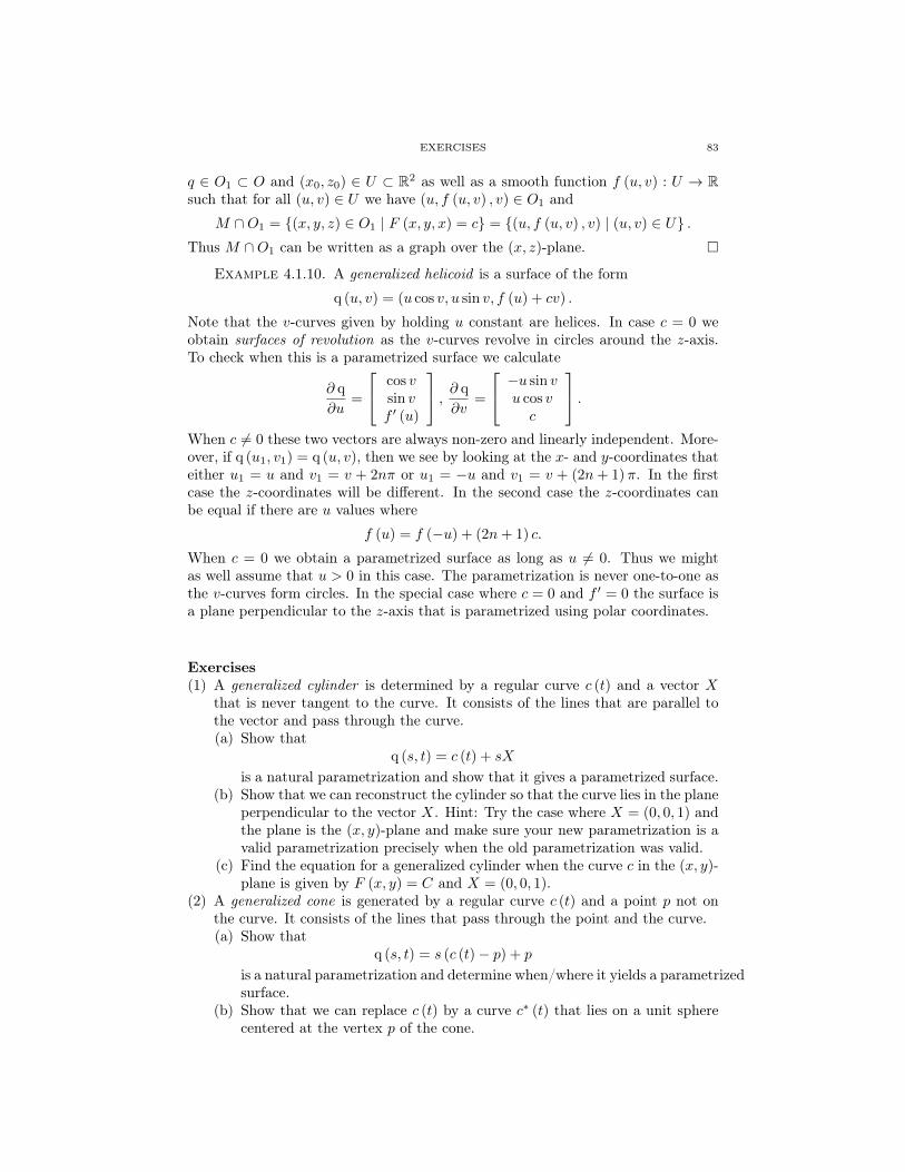
EXERCISES 83
q ∈ O1 ⊂ O and (x0, z0) ∈ U ⊂ R2 as well as a smooth function f (u, v) : U → Rsuch that for all (u, v) ∈ U we have (u, f (u, v) , v) ∈ O1 and
M ∩O1 = (x, y, z) ∈ O1 | F (x, y, x) = c = (u, f (u, v) , v) | (u, v) ∈ U .Thus M ∩O1 can be written as a graph over the (x, z)-plane.
Example 4.1.10. A generalized helicoid is a surface of the form
q (u, v) = (u cos v, u sin v, f (u) + cv) .
Note that the v-curves given by holding u constant are helices. In case c = 0 weobtain surfaces of revolution as the v-curves revolve in circles around the z-axis.To check when this is a parametrized surface we calculate
∂ q
∂u=
cos vsin vf ′ (u)
, ∂ q
∂v=
−u sin vu cos vc
.When c 6= 0 these two vectors are always non-zero and linearly independent. More-over, if q (u1, v1) = q (u, v), then we see by looking at the x- and y-coordinates thateither u1 = u and v1 = v + 2nπ or u1 = −u and v1 = v + (2n+ 1)π. In the firstcase the z-coordinates will be different. In the second case the z-coordinates canbe equal if there are u values where
f (u) = f (−u) + (2n+ 1) c.
When c = 0 we obtain a parametrized surface as long as u 6= 0. Thus we mightas well assume that u > 0 in this case. The parametrization is never one-to-one asthe v-curves form circles. In the special case where c = 0 and f ′ = 0 the surface isa plane perpendicular to the z-axis that is parametrized using polar coordinates.
Exercises(1) A generalized cylinder is determined by a regular curve c (t) and a vector X
that is never tangent to the curve. It consists of the lines that are parallel tothe vector and pass through the curve.(a) Show that
q (s, t) = c (t) + sX
is a natural parametrization and show that it gives a parametrized surface.(b) Show that we can reconstruct the cylinder so that the curve lies in the plane
perpendicular to the vector X. Hint: Try the case where X = (0, 0, 1) andthe plane is the (x, y)-plane and make sure your new parametrization is avalid parametrization precisely when the old parametrization was valid.
(c) Find the equation for a generalized cylinder when the curve c in the (x, y)-plane is given by F (x, y) = C and X = (0, 0, 1).
(2) A generalized cone is generated by a regular curve c (t) and a point p not onthe curve. It consists of the lines that pass through the point and the curve.(a) Show that
q (s, t) = s (c (t)− p) + p
is a natural parametrization and determine when/where it yields a parametrizedsurface.
(b) Show that we can replace c (t) by a curve c∗ (t) that lies on a unit spherecentered at the vertex p of the cone.

EXERCISES 84
(c) Show that the level set F (x, y, z) = 0 is a cone through the origin whenF is homogeneous, i.e., there is an α 6= 0 such that F (λx, λy, λz) =λαF (x, y, z).
(d) Further show that the condition for the cone in (c) to be a smooth surfaceaway from the origin is that∇F (q) is not proportional to q, when F (q) = 0.
(3) A ruled surface is given by a parametrization of the form
q (s, t) = c (t) + sX (t) .
It is evidently a surface that is a union of lines (rulers) and generalizes the con-structions in the previous exercises. Give conditions on c,X and the parameters that guarantee we get a parametrized surface. A special case occurs when Xis tangent to c. These are also called tangent developables.
(4) A surface of revolution is determined by a planar regular curve and a line inthe same plane. The surface is generated by rotating the curve around the line.(a) Show that for a regular curve (r (t) , z (t)) in the (x, z)- plane that is rotated
around the z-axis the parametrization is
q (t, µ) = (r (t) cosµ, r (t) sinµ, z (t))
and show that it is a parametrized surface.(b) Show that the equation for the surface is F
(√x2 + y2, z
)= c when the
curve is given by F (r, z) = c with x > 0.(c) Show that the equation for the surface is given by R2 (z) = x2 + y2, when
the curve can be written as r = R (z).(5) Let q (z, µ) =
(√1− z2 cosµ,
√1− z2 sinµ, z
)with −1 < z < 1 and −π < µ <
π. Show that q defines a surface. What is the surface?(6) Consider a regular curve c (t) with non-vanishing curvature and construct the
tube of radius R around it
q (t, φ) = c (t) +R (Nc cosφ+ Bc sinφ) ,
where Nc, Bc are the normal and binormal to the curve.(a) Show that this defines a parametrized surface as long as κc < R−1.(b) Show by example that this surface might intersect itself if there is a cord
of length < 2R that is normal to the curve at both end points.(c) Show that when c is a circle, then we obtain a surface of revolution that
looks like a torus.(7) Consider the level set:
z(x2 + y2
)− 2xy = R.
(a) Show that this defines a surface when R 6= 0.(b) When R = 0 show that we get a surface as long as (x, y) 6= (0, 0). This is
called Plücker’s conoid.(c) When R = 0 show that it is a ruled surface. Hint: Use polar coordinates
x = t cos θ and y = t sin θ.(8) Show that (
x2 + y2 + z2 +R2 − r2)2
= 4R2(x2 + y2
)defines a surface when R > r > 0. Show that it is rotationally symmetric anda torus, i.e., it is a parametrized circle rotated around the z-axis.

EXERCISES 85
(9) The helicoid is given by the equation
tanz
h=y
x
where h 6= 0 is a fixed constant.(a) Show that this defines a surface for suitable (x, y, z).(b) Show that the surface can be parametrized by
q (r, θ) = (r cos θ, r sin θ, hθ)
and determine for which r, θ this defines a parametrized surface. Note thatfor fixed r we obtain helices.
(10) Enneper’s surface is defined by the parametrization
q (u, v) =
(u− 1
3u3 + uv2, v − 1
3v3 + vu2, u2 − v2
).
(a) For which u, v does this define a parametrization?(b) Show that Enneper’s surface satisfies the equation(
y2 − x2
2z+
2z2
9+
2
3
)3
= 6
(y2 − x2
4z− 1
4
(x2 + y2 +
8
9z2
)+
2
9
)2
.
(11) Show that there exists a parametrization q : U → S2 ⊂ R3 that covers theentire sphere. Hint: If U is the disjoint union of two discs, then this can bedone using two maps that each cover a region slightly larger than a hemisphere.Now connect these discs by a band in R2 and similarly in the sphere to obtaina parametrization from a domain U that is diffeomorphic to R2.
(12) Many classical surfaces are of the form
F (x, y, z) = ax2 + by2 + cz2 + dx+ ey + fz + g = 0.
These are called quadratic surfaces if one of a, b, or c 6= 0.(a) Show that it is either empty or defines a surface at points (x, y, z) ∈ R3−C,
where C is the closed set defined by
C = (x, y, z) | 2ax = −d, 2by = −e, 2cz = −f .
(b) Show that C is either empty, a point, a line, or a plane.(c) Under what conditions does it become a surface of revolution around the
z-axis?(d) Show that when the equation does not depend on one of the coordinates,
then we obtain a generalized cylinder.(e) When, say c = 0, but abf 6= 0 we obtain a paraboloid. It is elliptic when
a, b have the same sign and otherwise hyperbolic. Draw pictures of thesetwo situations.
(f) When abc 6= 0 show that it can be rewritten in the form
F (x, y, z) = a (x− x0)2
+ b (y − y0)2
+ c (z − z0)2
+ h = 0.
(g) When all three a, b, c have the same sign show that it is either empty or anellipsoid.
(h) When not all of a, b, c have the same sign and h 6= 0 we obtain a hyperboloid.Show that it might be connected or have two components (called sheets)depending of the signs of all four constants.
(i) When not all of a, b, c have the same sign and h = 0 we obtain a cone.

4.2. TANGENT SPACES AND MAPS 86
(j) Given constants ax, ay, az determine when
q (u, v) = (ax cosu cos v, ay cosu sin v, az sinu) ,
q (u, v) = (ax sinhu cos v, ay sinhu sin v, az coshu) ,
q (u, v) = (ax coshu cos v, ay coshu sin v, az sinhu) ,
q (u, v) =(axu cos v, ayu sin v, azu
2),
q (u, v) =(axu cosh v, ayu sinh v, azu
2),
yield parametrizations and identify them with the appropriate quadratics.
4.2. Tangent Spaces and Maps
Definition 4.2.1. The tangent space at q ∈ M of a (parametrized) surface isdefined as
TqM = span
∂ q
∂u,∂ q
∂v
,
and normal space is the orthogonal complement
NqM = (TqM)⊥.
Remark 4.2.2. For a parametrized surface with self-intersections this is a bitambivalent as the tangent space in that case depends on the parameter values (u, v)and not just the point q = q (u, v). This is just as for curves where the tangent lineat a point really is the tangent line at a point with respect to a specific parametervalue.
Remark 4.2.3. Note that the tangent and normal spaces are subspaces. We canalso define the tangent plane at q ∈M , as the plane parallel to TqM that containsq. The tangent plane is then similar to the tangent line for a curve. Similarly, thenormal line to q ∈ M is the line through q that is parallel to NqM . A normal toM at q is a choice of a unit vector in n ∈ NqM . There are two normals at eachpoint. In the rest of these notes n will always denote a unit normal to a surface.The principal normal to a curve c will be denoted Nc.
Example 4.2.4. A parametrized surface q (u, v) : U → R3 always has a naturalnormal n (u, v) defined by
n (u, v) =∂ q∂u ×
∂ q∂v∣∣∣∂ q
∂u ×∂ q∂v
∣∣∣However, it is possible (as well shall see in the exercises) that there are parametervalues that give the same points and tangent spaces to the surface without givingthe same normal vectors.
Example 4.2.5 (Example 4.1.10 continued). The normal of the generalizedhelicoid is given by
n (u, v) =∂ q∂u ×
∂ q∂v∣∣∣∂ q
∂u ×∂ q∂v
∣∣∣ =1√
c2 + u2(
1 + (f ′)2) c sin v − uf ′ cos v−c cos v − uf ′ sin v
u
.Proposition 4.2.6. Both tangent and normal spaces are subspaces that do not
change under reparametrization.

4.2. TANGENT SPACES AND MAPS 87
Proof. This would seem intuitively clear, just as with curves, where the tan-gent line does not depend on parametrizations. For curves it boils down to thesimple fact that velocities for different parametrizations are proportional. Withsurfaces something similar happens, but it is a bit more involved. Suppose we havetwo different parametrizations of the same surface:
q (s, t) = q (u, v) .
This tells us that the parameters are functions of each other
u = u (s, t) , v = v (s, t) ,
s = s (u, v) , t = t (u, v) .
The chain rule then gives us∂ q
∂u=∂ q
∂s
∂s
∂u+∂ q
∂t
∂t
∂u∈ span
∂ q
∂s,∂ q
∂t
,
and∂ q
∂v∈ span
∂ q
∂s,∂ q
∂t
.
In the other direction we similarly have∂ q
∂s,∂ q
∂t∈ span
∂ q
∂u,∂ q
∂v
.
This shows that at a fixed point q on a surface, the tangent space does not dependon how the surface is parametrized. The normal space is then also well-defined.
Note that the chain rule shows in matrix notation that[∂ q∂u
∂ q∂v
]=
[∂ q∂s
∂ q∂t
] [ ∂s∂u
∂s∂v
∂t∂u
∂t∂v
],
[∂ q∂s
∂ q∂t
]=
[∂ q∂u
∂ q∂v
] [ ∂u∂s
∂u∂t
∂v∂s
∂v∂t
]with [
∂s∂u
∂s∂v
∂t∂u
∂t∂v
]−1
=
[∂u∂s
∂u∂t
∂v∂s
∂v∂t
].
A better way of defining the tangent space that also shows that it is independentof parametrizations comes from the next result.
Proposition 4.2.7. The tangent space at q = q (u0, v0) for a (parametrized)surface is given by
TqM =
v ∈ R3 | v =
d q
dt(0) for a smooth curve q (t) : I →M with q (0) = q
.
Proof. Any curve q (t) on the surface that passes through q at t = 0 can bewritten as
q (t) = q (u (t) , v (t))
for smooth functions u (t) and v (t) with u (0) = u0 and v (0) = v0 as long as t issufficiently small. This is because the parametrization is locally one-to-one. If wewrite the curve this way, then
d q
dt=∂ q
∂u
du
dt+∂ q
∂v
dv
dt.

4.2. TANGENT SPACES AND MAPS 88
Showing that velocities of curves on the surface are always tangent vectors. Con-versely by using u (t) = at + u0 and v (t) = bt + v0 we obtain all possible linearcombinations of tangent vectors as
d q
dt(0) =
∂ q
∂ua+
∂ q
∂vb.
Corollary 4.2.8. Let M = (x, y, z) ∈ O | F (x, y, z) = c be a level set as intheorem 4.1.9. The normal space is spanned by
∇F (q) =
∂F∂x (q)∂F∂y (q)∂F∂z (q)
.Proof. We saw in proposition 4.2.7 that any tangent vector in TqM can be
represented as a velocity vector q (0). Since q (t) ∈ M it follows that F (q (t)) = cfor all t. The chain rule then implies that
0 = ∇F (q (0)) · q (0) = ∇F (q) · q (0) .
This shows that the gradient is perpendicular to all tangent vectors and hence anormal vector.
Example 4.2.9. The sphere of radius R centered at the origin has a unit normalgiven by the unit radial vector at q = (x, y, z) ∈ S2 (R)
n =1
Rq =
1
R
xyz
.The basis for the tangent space with respect to the meridian/latitude parametriza-tion is
∂ q
∂µ= R
− sinµ cosφcosµ cosφ
0
, ∂ q
∂φ= R
− cosµ sinφ− sinµ sinφ
cosφ
.It is often useful to find coordinates suited to a particular situation. However,
unlike for curves, it isn’t always possible to parametrize a surface such that thecoordinate curves are unit speed and orthogonal to each other. But there is onegeneral construction we can do.
Theorem 4.2.10. Assume that we have linearly independent tangent vectorfields X,Y defined on a surface M. Then it is possible to find a parametrizationq (u, v) in a neighborhood of any point such that ∂ q
∂u is proportional to X and ∂ q∂v is
proportional to Y.
Proof. The vector fields have integral curves forming a net on the surface.Apparently the goal is to reparametrize the curves in this net in some fashion. Thedifficulty lies in ensuring that the levels where u is constant correspond to the v-curves, and vice versa. We proceed as with the classical construction of Cartesiancoordinates. Select a point p and let the u-axis be the integral curve for X throughp, similarly let the v-axis be the integral curve for Y through p. Both of these curvesretain the parametrizations that make them integral curves forX and Y. Thus p willnaturally correspond to (u, v) = (0, 0) . We now wish to assign (u, v) coordinatesto a point q near p. There are also unique integral curves for X and Y through

4.2. TANGENT SPACES AND MAPS 89
q. These will be our way of projecting onto the chosen axes and will in this wayyield the desired coordinates. Specifically, u (q) is the parameter where the integralcurve for Y through q intersects the u-axis, and similarly with v (q) . In general,integral curves can intersect axes in several places or might not intersect them atall. However, a continuity argument offers some justification when we consider thatthe axes themselves are the proper integral curves for the qs that lie on these axesand so when q sufficiently close to both axes it should have a well-defined set ofcoordinates. We also note that as the projection happens along integral curveswe have ensured that coordinate curves are simply reparametrizations of integralcurves. To completely justify this construction we need to know quite a bit aboutthe existence, uniqueness and smoothness of solutions to differential equations andthe inverse function theorem.
Remark 4.2.11. Note that this proof gives us a little more information. Specif-ically, we obtain a parametrization where the parameter curves through (0, 0) arethe integral curves for X and Y .
Definition 4.2.12. A map between surfaces F : M1 → M2 is an assignmentof points in the first surface to points in the second. The map is smooth if aroundevery point q ∈ M1 we can find a parametrization q1 (u, v) where q = q1 (u0, v0)such that the composition F q1 : U → R3 is a smooth map as a map from thespace of parameters to the ambient space that contains the target M2.
We can also define maps between parametrized surfaces in a similar way.Clearly parametrizations are themselves smooth maps. It is also often the casethat the compositions F q1 are themselves parametrizations for M2.
Example 4.2.13. Two classical examples of maps are the Archimedes and Mer-cator projections from the sphere to the cylinder of the same radius placed to touchthe sphere at the equator. We give the formulas for the unit sphere and note thatneither map is defined at the poles.
The Archimedes map is simply a horizontal projection that preserves the z-coordinate
A
xyz
=
x√x2+y2y√x2+y2
z
.In the meridian/latitude parametrization it looks particularly nice:
A
cosµ cosφsinµ cosφ
sinφ
=
cosµsinµsinφ
.Note that what is here referred to as the Archimedes map is often called the Lambertprojection. However, Archimedes was the first to discover that the areas of thesphere and cylinder are equal. This will be discussed in greater detail in section4.4.
The Mercator projection (1569) differs in that the z-coordinate is not preserved:
M
xyz
=
x√x2+y2y√x2+y2
12 log 1+z
1−z

4.2. TANGENT SPACES AND MAPS 90
or
M
cosµ cosφsinµ cosφ
sinφ
=
cosµsinµ
12 log 1+sinφ
1−sinφ
.Both of these maps really are maps in the traditional sense that they can be
used to picture the Earth on a flat piece of paper by cutting the cylinder verticallyand unfolding it. This unfolding is done along a meridian. For Eurocentric peopleit is along the date line. In the Americas one also sees maps cut along a meridianthat bisects Asia so as to place the Americas in the center.
Definition 4.2.14. The differential of a smooth map F : M1 →M2 at q ∈M1
is the mapDFq : TqM1 → TF (q)M2
defined by
DFq (v) =dF q
dt(0)
if q (t) is a curve (in M1) with q = q (0) and v = d qdt (0).
Proposition 4.2.15. When v = d qdt (0) = ∂ q
∂u vu +∂ q∂v vv we have
DFq (v) =[∂Fq∂u
∂Fq∂v
] [ vu
vv
].
In particular, the differential is a linear map and is completely determined by thetwo partial derivatives ∂Fq
∂u , ∂Fq∂v .
Proof. This follows from the chain rule:dF q
dt(t) =
dF (q (t))
dt
=dF (q (u (t) , v (t)))
dt
=∂F q
∂u
du
dt+∂F q
∂v
dv
dt
=[∂Fq∂u
∂Fq∂v
] [ dudtdvdt
].
Example 4.2.16. The Archimedes map satisfies
∂ (A q)
∂µ=
− sinµcosµ
0
, ∂ (A q)
∂φ=
00
− cosφ
and the Mercator map
∂ (M q)
∂µ=
− sinµcosµ
0
, ∂ (M q)
∂φ=
001
cosφ
.Definition 4.2.17. A surfaceM is orientable if we can select a smooth normal
field. Thus we require a smooth function
n : M → S2 (1) ⊂ R3
EXERCISES 91
such that for all q ∈M the vector n (q) is perpendicular to the tangent space TqM .The map n : M → S2 (1) is called the Gauss map.
Proposition 4.2.18. A surface which is given as a level set is orientable.
Proof. Form corollary 4.2.8 we know that the normal can be given by
n =∇F|∇F |
if M = q ∈ O | F (q) = c.
Definition 4.2.19. The parameters u, v on a parameterized surface q (u, v)define two differentials du and dv. These are not mysterious infinitesimals, butlinear functions on tangent vectors to the surface that compute the coefficients ofthe vector with respect to the basis ∂ q
∂u ,∂ q∂v . Thus
du (v) = du
(∂ q
∂uvu +
∂ q
∂vvv)
= vu,
dv (v) = dv
(∂ q
∂uvu +
∂ q
∂vvv)
= vv,
and
v =[∂ q∂u
∂ q∂v
] [ dudv
](v) =
[∂ q∂u
∂ q∂v
] [ vu
vv
].
From the chain rule we obtain the very natural transformation laws for differ-entials
du =∂u
∂sds+
∂u
∂tdt,
dv =∂v
∂sds+
∂v
∂tdt,
or [dudv
]=
[∂u∂s
∂u∂t
∂v∂s
∂v∂t
] [dsdt
].
Exercises(1) Show that the following conditions for a surface are equivalent:
(a) It is part of a plane.(b) The normal vector is constant.(c) All the tangent planes are parallel.
(2) Show that the following conditions for a surface are equivalent:(a) It is part of a sphere.(b) All normal lines pass through a fixed point.(c) n = λ (q−c) for some function λ and point c. Hint: Select a parametriza-
tion, show that ∂n∂w is a tangent vector for w = u, v, and use this to show
that λ must be constant.(3) Show that the ruled surface
q (t, φ) = (cosφ, sinφ, 0) + t
(sin
φ
2cosφ, sin
φ
2sinφ, cos
φ
2
)

EXERCISES 92
defines a parametrized surface. It is called the Möbius band. Show that it isnot orientable by showing that when t = 0 and φ = ±π we obtain the samepoint and tangent space on the surface, but the normals
n (t, φ) =
∂ q∂t ×
∂ q∂φ∣∣∣∂ q
∂t ×∂ q∂φ
∣∣∣are not the same.
(4) Show that q (t, φ) = t (cosφ, sinφ, 1) defines a parametrization for (t, φ) ∈(0,∞)×R. Show that the corresponding surface is x2+y2−z2 = 0, z > 0. Showthat this parametrization is not one-to-one. Find a different parametrizationof the entire surface that is one-to-one.
(5) Consider the two surfaces M1 and M2 defined by the parametrizations:
q1 (t, φ) = (sinhφ cos t, sinhφ sin t, t)
= (0, 0, t) + sinhφ (cos t, sin t, 0) ,
q2 (t, φ) = (cosh t cosφ, cosh t sinφ, t) .
(a) Show that q1 : R × R → M1 is a one-to-one parametrization of a helicoid(see section 4.1 exercise 9).
(b) Show that q2 is a parametrization that is not one-to-one. Show that M2 isrotationally symmetric (see section 4.1 exercise 4) and can also be describedby the equation
x2 + y2 = cosh2 z.
Show further that this equation defines a surface. It is called the catenoid.(c) Define a map F : M1 →M2 by F q1 (t, φ) = q2 (t, φ). Show that this map
is smooth, not one-to-one, but locally a diffeomorphism.(6) Show that a parametrized surface
q (z, θ) =
r (z, θ) cos θr (z, θ) sin θ
z
is rotationally symmetric, i.e., ∂r∂θ = 0, if all its normal lines pass through thez-axis.
(7) The inversion in the unit sphere or circle is defined as
F (q) =q
|q|2.
(a) Show that this is a diffeomorphism of Rn − 0 to it self with the propertythat q · F (q) = 1.
(b) Show that F preserves the unit sphere, but reverses the unit normal direc-tions.
(c) LetM be a surface. Show thatM∗ = F (M) defines another surface. Showthat DF : TqM → Tq∗M
∗ satisfies
DF (v) =|q|2 v − 2(q · v)q
|q|4.

4.3. THE FIRST FUNDAMENTAL FORM 93
(d) Show that if n is a unit normal to M , then the unit normal to M∗ is givenby
n∗ = ±
(n−q 2q · n
|q|2
).
(8) A perspective projection is defined as a radial projection along lines emanatingfrom a fixed point c ∈ Rn to a hyper-plane H ⊂ Rn.(a) Let c = (0, 0, c) ∈ R3 and H be the (x, y)-plane. Show that the projection
is given by (x, y, z) 7→(cxc−z ,
cyc−z , 0
).
(b) Let c = (0, 0, 0) ∈ R3 andH be the z = 1-plane. Show that the projectionis given by (x, y, z) 7→
(xz ,
yz , 1).
(c) Let c = (0, 0, 1) ∈ R3 and H be the z = −1-plane. Show that the pro-jection is given by (x, y, z) 7→
(2x
1−z ,2y
1−z ,−1).
(9) Consider the two maps q± : Rn → Rn × R = Rn+1
q± (q) = (q, 0) +1− |q|2
1 + |q|2(q,±1) .
These two maps are inverses of perspective projections to the unit sphere. Theyare also called stereographic projections.(a) Show that these maps are one-to-one, map into the unit sphere, and that
together they cover the unit sphere.(b) Show that they are the inverse maps of the perspective projections from
(0,∓1) ∈ Rn × R to the Rn ⊂ Rn × R plane where the last coordinatevanishes.
(c) Show that q+(
q|q|2
)= q− (q) and q+ (q) = q−
(q|q|2
).
4.3. The First Fundamental Form
Let q (u, v) : U → R3 be a parametrized surface. At each point of this surfacewe have a basis
∂ q
∂u(u, v) ,
∂ q
∂v(u, v) ,
n (u, v) =∂ q∂u ×
∂ q∂v∣∣∣∂ q
∂u ×∂ q∂v
∣∣∣ .These vectors are again parametrized by u, v. The first two vectors are tangentto the surface and give us an unnormalized version of the tangent vector for acurve, while the third is the normal and is naturally normalized just as the normalvector is for a curve. One of the issues that make surface theory more difficult thancurve theory is that there is no canonical parametrization such as the arclengthparametrization for curves.

4.3. THE FIRST FUNDAMENTAL FORM 94
The first fundamental form is the symmetric positive definite form that comesfrom the matrix
[I] =[∂ q∂u
∂ q∂v
]t [ ∂ q∂u
∂ q∂v
]=
[∂ q∂u ·
∂ q∂u
∂ q∂u ·
∂ q∂v
∂ q∂v ·
∂ q∂u
∂ q∂v ·
∂ q∂v
]=
[guu guvgvu gvv
].
For a curve the analogous term would simply be the square of the speed(d q
dt
)td q
dt=d q
dt· d q
dt.
The first fundamental form dictates how one computes dot products of vectorstangent to the surface assuming they are expanded according to the basis ∂ q
∂u ,∂ q∂v .
If
X = Xu ∂ q
∂u+Xv ∂ q
∂v=[∂ q∂u
∂ q∂v
] [ Xu
Xv
],
Y = Y u∂ q
∂u+ Y v
∂ q
∂v=[∂ q∂u
∂ q∂v
] [ Y u
Y v
],
then
I (X,Y ) =[Xu Xv
] [ guu guvgvu gvv
] [Y u
Y v
]=
[Xu Xv
] [∂ q∂u
∂ q∂v
]t [ ∂ q∂u
∂ q∂v
] [ Y u
Y v
]=
([∂ q∂u
∂ q∂v
] [ Xu
Xv
])t([∂ q∂u
∂ q∂v
] [ Y u
Y v
])= XtY
= X · Y.In particular, we see that while themetric coefficients gw1w2
depend on our parametriza-tion, the dot product I (X,Y ) of two tangent vectors remains the same if we changeparameters. Note that I stands for the bilinear form I (X,Y ) which does not de-pend on parametrizations, while [I] is the matrix representation with respect to aparametrization.
Our first observation is that the normalization factor∣∣∣∂ q∂u ×
∂ q∂v
∣∣∣ can be com-puted from [I] .
Definition 4.3.1. The area form of a parametrized surface is given by√det [I].
The next lemma shows that this is given by the area of the parallelogramspanned by ∂ q
∂u ,∂ q∂v .
Lemma 4.3.2. We have∣∣∣∣∂ q
∂u× ∂ q
∂v
∣∣∣∣2 = det [I] = guugvv − (guv)2.

4.3. THE FIRST FUNDAMENTAL FORM 95
Proof. This is simply the observation that both sides of the equation areformulas for the square of the area of the parallelogram spanned by ∂ q
∂u ,∂ q∂v , i.e.,∣∣∣∣∂ q
∂u× ∂ q
∂v
∣∣∣∣2 =
∣∣∣∣∂ q
∂u
∣∣∣∣2 ∣∣∣∣∂ q
∂v
∣∣∣∣2 − (∂ q
∂u· ∂ q
∂v
)2
.
Example 4.3.3 (Example 4.1.10 continued). The first fundamental form andarea form of the generalized helicoid are given by
[I] =
[1 + (f ′)
2cf ′
cf ′ u2 + c2
], det [I] = c2 + u2
(1 + (f ′)
2).
Example 4.3.4. We also need to know how the first fundamental form changesunder a reparametrization. Consider for example (u, v) = er (cos θ, sin θ) so that
∂ q
∂r=∂ q
∂u
∂u
∂r+∂ q
∂v
∂v
∂r=∂ q
∂uer cos θ +
∂ q
∂ver sin θ,
∂ q
∂θ=∂ q
∂u
∂u
∂θ+∂ q
∂v
∂v
∂θ= −∂ q
∂uer sin θ +
∂ q
∂ver cos θ.
Thus
grr =
(∂ q
∂u
∂u
∂r+∂ q
∂v
∂v
∂r
)·(∂ q
∂u
∂u
∂r+∂ q
∂v
∂v
∂r
)= guu
∂u
∂r
∂u
∂r+ 2guv
∂u
∂r
∂v
∂r+ gvv
∂v
∂r
∂v
∂r
= e2r(guu cos2 θ + 2guv cos θ sin θ + gvv sin2 θ
),
grθ =
(∂ q
∂u
∂u
∂r+∂ q
∂v
∂v
∂r
)·(∂ q
∂u
∂u
∂θ+∂ q
∂v
∂v
∂θ
)= guu
∂u
∂r
∂u
∂θ+ guv
(∂u
∂r
∂v
∂θ+∂u
∂θ
∂v
∂r
)+ gvv
∂v
∂r
∂v
∂θ
= e2r(−guu cos θ sin θ + guv
(cos2 θ − sin2 θ
)+ gvv cos θ sin θ
),
gθθ =
(∂ q
∂u
∂u
∂θ+∂ q
∂v
∂v
∂θ
)·(∂ q
∂u
∂u
∂θ+∂ q
∂v
∂v
∂θ
)= guu
∂u
∂θ
∂u
∂θ+ 2guv
∂u
∂θ
∂v
∂θ+ gvv
∂v
∂θ
∂v
∂θ
= e2r(guu sin2 θ − 2guv sin θ cos θ + gvv cos2 θ
).
In matrix notation[grr grθgθr gθθ
]=
[∂u∂r
∂u∂θ
∂v∂r
∂v∂θ
]t [guu guvgvu gvv
] [∂u∂r
∂u∂θ
∂v∂r
∂v∂θ
]=
[∂u∂r
∂v∂r
∂u∂θ
∂v∂θ
] [guu guvgvu gvv
] [∂u∂r
∂u∂θ
∂v∂r
∂v∂θ
].
The inverse matrix
[I]−1
=
[guu guvgvu gvv
]−1
=
[guu guv
gvu gvv
]can be used to find the expansion of a tangent vector by computing its dot productswith the basis:

4.3. THE FIRST FUNDAMENTAL FORM 96
Proposition 4.3.5. If X ∈ TqM, then
X =
(guu
(X · ∂ q
∂u
)+ guv
(X · ∂ q
∂v
))∂ q
∂u
+
(gvu
(X · ∂ q
∂u
)+ gvv
(X · ∂ q
∂v
))∂ q
∂v
=[∂ q∂u
∂ q∂v
][I]−1 [ ∂ q
∂u∂ q∂v
]tX.
More generally, for any Z ∈ R3
Z =
(guu
(Z · ∂ q
∂u
)+ guv
(Z · ∂ q
∂v
))∂ q
∂u
+
(gvu
(Z · ∂ q
∂u
)+ gvv
(Z · ∂ q
∂v
))∂ q
∂v+ (Z · n) n
=[∂ q∂u
∂ q∂v
][I]−1 [ ∂ q
∂u∂ q∂v
]tZ + (Z · n) n .
Proof. This formula works for X ∈ TqM by writing
X =[∂ q∂u
∂ q∂v
] [ Xu
Xv
]= Xu ∂ q
∂u+Xv ∂ q
∂v
and then observing that[∂ q∂u
∂ q∂v
][I]−1 [ ∂ q
∂u∂ q∂v
]tX =
[∂ q∂u
∂ q∂v
][I]−1 [ ∂ q
∂u∂ q∂v
]t [ ∂ q∂u
∂ q∂v
] [ Xu
Xv
]=
[∂ q∂u
∂ q∂v
][I]−1
[I]
[Xu
Xv
]=
[∂ q∂u
∂ q∂v
] [ Xu
Xv
]= X.
For a general vector Z ∈ R3 the result follows by using the orthogonal decomposition
Z = X + (Z · n) n,
where X = Z − (Z · n) n ∈ TqM and observing that the operation
Z 7→[∂ q∂u
∂ q∂v
][I]−1 [ ∂ q
∂u∂ q∂v
]tZ
is a linear map defined for all Z ∈ R3 with kernel spanned by n. In fact, itorthogonally projects Z to TqM .
Defining the gradient of a function is another important use of the first funda-mental form as well as its inverse. Let f (u, v) be viewed as a function on the surfaceq (u, v) . Our definition of the gradient should definitely be so that it conforms withthe chain rule for a curve q (t) = q (u (t) , v (t)) . Thus on one hand we want
d (f q)
dt= ∇f · q
=[
(∇f)u
(∇f)v ]
[I]
[dudtdvdt
]while the chain rule also dictates
d (f q)
dt=[∂f∂u
∂f∂v
] [ dudtdvdt
].

EXERCISES 97
This indicates that [(∇f)
u(∇f)
v ]=[∂f∂u
∂f∂v
][I]−1
or
∇f =[∂ q∂u
∂ q∂v
] [ (∇f)u
(∇f)v
]=
[∂ q∂u
∂ q∂v
] ([∂f∂u
∂f∂v
][I]−1)t
=[∂ q∂u
∂ q∂v
][I]−1 [ ∂f
∂u∂f∂v
]t=
(guu
∂f
∂u+ guv
∂f
∂v
)∂ q
∂u+
(gvu
∂f
∂u+ gvv
∂f
∂v
)∂ q
∂v.
In particular, we see that changing coordinates changes the gradient in such a waythat it isn’t simply the vector corresponding to the partial derivatives! The othernice feature is that we now have a concept of the gradient that gives a vector fieldindependently of parametrizations. The defining equation
d (f q)
dt= ∇f · q = I (∇f, q)
gives an implicit definition of∇f that makes sense without reference to parametriza-tions of the surface.
Exercises(1) For a surface of revolution q (t, µ) = (r (t) cosµ, r (t) sinµ, z (t)) (see section 4.1
exercise 4) show that the first fundamental form is given by[gtt gtµgµt gµµ
]=
[r2 + z2 0
0 r2
].
A special and important case of this occurs when z = 0 and r = t as thatcorresponds to polar coordinates in the (x, y)-plane.
(2) Assume that we have a cone (see section 4.1 exercise 2) given by
q (r, φ) = rc (φ) ,
where c is a space curve with |c| = 1 and∣∣∣ dcdφ ∣∣∣ = 1. Show that the first
fundamental form is given by[grr grφgφr gφφ
]=
[1 00 r2
]and compare this to polar coordinates in the plane.
(3) Assume that we have a generalized cylinder (see section 4.1 exercise 1) givenby
q (s, t) = (x (s) , y (s) , t) ,
where (x (s) , y (s)) is unit speed. Show that the first fundamental form is givenby [
gss gstgts gtt
]=
[1 00 1
].
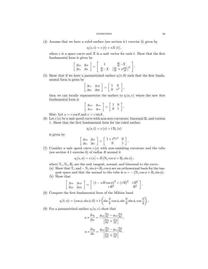
EXERCISES 98
(4) Assume that we have a ruled surface (see section 4.1 exercise 3) given by
q (s, t) = c (t) + sX (t) ,
where c is a space curve and X is a unit vector for each t. Show that the firstfundamental form is given by[
gss gstgts gtt
]=
[1 dc
dt ·Xdcdt ·X
∣∣dcdt + sdXdt
∣∣2].
(5) Show that if we have a parametrized surface q (r, θ) such that the first funda-mental form is given by[
grr grθgθr gθθ
]=
[1 00 r2
],
then we can locally reparametrize the surface to q (u, v) where the new firstfundamental form is [
guu guvgvu gvv
]=
[1 00 1
].
Hint: Let u = r cos θ and v = r sin θ.(6) Let c (s) be a unit speed curve with non-zero curvature, binormal Bc and torsion
τ . Show that the first fundamental form for the ruled surface
q (s, t) = c (s) + tBc (s)
is given by [gss gstgts gtt
]=
[1 + t2τ2 0
0 1
].
(7) Consider a unit speed curve c (s) with non-vanishing curvature and the tube(see section 4.1 exercise 6) of radius R around it
q (s, φ) = c (s) +R (Nc cosφ+ Bc sinφ) ,
where Tc,Nc,Bc are the unit tangent, normal, and binormal to the curve.(a) Show that Tc and −Nc sinφ+Bc cosφ are an orthonormal basis for the tan-
gent space and that the normal to the tube is n = − (Nc cosφ+ Bc sinφ).(b) Show that[
gss gsφgφs gφφ
]=
[(1− κR cosφ)
2+ (τR)
2τR2
τR2 R2
].
(8) Compute the first fundamental form of the Möbius band
q (t, φ) = (cosφ, sinφ, 0) + t
(sin
φ
2cosφ, sin
φ
2sinφ, cos
φ
2
).
(9) For a parametrized surface q (u, v) show that
n×∂ q
∂u=guu
∂ q∂v − guv
∂ q∂u∣∣∣∂ q
∂u ×∂ q∂v
∣∣∣ ,
n×∂ q
∂v=guv
∂ q∂v − gvv
∂ q∂u∣∣∣∂ q
∂u ×∂ q∂v
∣∣∣ .

EXERCISES 99
(10) Assume a surface has a parametrization q (s, µ) where[gss gsµgµs gµµ
]=
[1 00 r2
],
where r (s) is only a function of s.(a) Show that if 0 < dr
ds < 1, then there is a function z (s) so that (r (s) , 0, z (s))is a unit speed curve.
(b) Conclude that there is a surface of revolution with the same first funda-mental form.
(11) Assume a surface has a parametrization q (u, v) where[guu guvgvu gvv
]=
[r2 00 r2
],
where r (u) > 0 is only a function of u. Show that there is a reparametrizationu = u (s) such that the first fundamental form becomes[
gss gsvgvs gvv
]=
[1 00 r2
].
(12) Show that if we have a parametrization where
[I] =
[1 00 gvv
],
then the coordinate function f (u, v) = u has
∇u =∂ q
∂u.
(13) Show that it is always possible to find an orthogonal parametrization, i.e., guvvanishes. Hint: Use theorem 4.2.10.
(14) Show that if∂guu∂v
=∂gvv∂u
= guv = 0,
then we can reparametrize u and v separately, i.e., u = u (s) and v = v (t) , insuch a way that we obtain Cartesian coordinates:
gss = gtt = 1,
gst = 0.
(15) Show that if∂2 q
∂u∂v= 0,
thenq (u, v) = F (u) +G (v) ,
and conclude that∂guu∂v
=∂gvv∂u
= 0.
Give an example where guv 6= 0.

4.4. SPECIAL MAPS AND PARAMETRIZATIONS 100
4.4. Special Maps and Parametrizations
Definition 4.4.1. We call a map F : M1 →M2 between surfaces an isometryif its differential preserves the first fundamental form
I1 (X,Y ) = I2 (DF (X) , DF (Y )) .
We call the map area preserving if it preserves the areas of parallelogramsspanned by vectors:
det
[I1 (X,X) I1 (X,Y )I1 (X,Y ) I1 (Y, Y )
]= det
[I1 (DF (X) , DF (X)) I1 (DF (X) , DF (Y ))I1 (DF (X) , DF (Y )) I1 (DF (Y ) , DF (Y ))
].
We call the map conformal if it preserves angles between vectors:
cos∠ (X,Y ) =I1 (X,Y )
|X|1 |Y |1=
I2 (DF (X) , DF (Y ))
|DF (X)|2 |DF (Y )|2.
When the first surface is given as a parametrized surface these conditions canbe checked as follows.
Proposition 4.4.2. Let q : U → M1 be a parametrization and F : M1 → M2
a map. The map is an isometry if
[I1] = [I2] ,
area preserving if
det [I1] = det [I2] ,
and conformal if
[I1] = λ2 [I2]
for some non-zero function λ.
Proof. Note that it is not necessary to first check that Fq is also a parametriza-tion as that will be a consequence of any one of the three conditions if we define
[I2] =
[∂Fq∂u ·
∂Fq∂u
∂Fq∂u ·
∂Fq∂v
∂Fq∂v ·
∂Fq∂u
∂Fq∂v ·
∂Fq∂v
]and observe that ∂Fq
∂v , ∂Fq∂u are linearly independent if and only if the matrix [I2]has nonzero determinant.
Next note that the chain rule implies that
DF
(∂ q
∂u
)=∂F q
∂u, DF
(∂ q
∂v
)=∂F q
∂v
So the three conditions are necessarily true if the map is an isometry, area preserv-ing, or conformal respectively. More generally, we see that
DF (X) = DF
(Xu ∂ q
∂u+Xv ∂ q
∂v
)= Xu ∂F q
∂u+Xv ∂F q
∂v.

4.4. SPECIAL MAPS AND PARAMETRIZATIONS 101
So if [I1] = [I2], then
I2 (DF (X) , DF (Y )) =[Xu Xv
] [∂Fq∂u
∂Fq∂v
]t [ ∂Fq∂u
∂Fq∂v
] [ Y u
Y v
]=
[Xu Xv
][I2]
[Y u
Y v
]=
[Xu Xv
][I1]
[Y u
Y v
]= I1 (X,Y ) .
A similar calculation with the assumption that [I1] = λ2 [I2] gives us
I1 (X,Y ) = λ2 I2 (X,Y ) ,
|X|2 = I1 (X,X) = λ2 I2 (X,X) ,
|Y |2 = I1 (Y, Y ) = λ2 I2 (Y, Y ) .
As angles are given by
cos∠ (X,Y ) =X · Y|X| |Y |
this establishes the last claim.Finally, if∣∣∣∣∂ q
∂u× ∂ q
∂v
∣∣∣∣2 = det [I1] = det [I2] =
∣∣∣∣∂F q
∂u× ∂F q
∂v
∣∣∣∣2 ,then the observation that
X × Y =
(Xu ∂ q
∂u+Xv ∂ q
∂v
)×(Y u
∂ q
∂u+ Y v
∂ q
∂v
)= (XuY v −XvY u)
∂ q
∂u× ∂ q
∂v,
DF (X)×DF (Y ) =
(Xu ∂F q
∂u+Xv ∂F q
∂v
)×(Y u
∂F q
∂u+ Y v
∂F q
∂v
)= (XuY v −XvY u)
∂F q
∂u× ∂F q
∂v,
shows that|X × Y |2 = |DF (X)×DF (Y )|2 .
The last statement can also be rephrased without the use of λ by checking that∂Fq∂u ·
∂Fq∂u
∂ q∂u ·
∂ q∂u
=∂Fq∂v ·
∂Fq∂v
∂ q∂v ·
∂ q∂v
and∂F q
∂v· ∂F q
∂u=
∂Fq∂u ·
∂Fq∂u
∂ q∂u ·
∂ q∂u
∂ q
∂v· ∂ q
∂u
Definition 4.4.3. In case the map is a parametrization q : U → M then wealways use the Cartesian metric on U given by[
1 00 1
].

4.4. SPECIAL MAPS AND PARAMETRIZATIONS 102
So the parametrization is an isometry or Cartesian when
[I] =
[1 00 1
],
area preserving whendet [I] = 1,
and conformal or isothermal when
guu = gvv,
guv = 0.
Example 4.4.4. It follows from proposition 4.4.2 and example 4.2.16 that theArchimedes map is area preserving and the Mercator map is conformal.
Example 4.4.5. Consider the reparametrization (u, v) = er (cos θ, sin θ) fromexample 4.3.4. If q (u, v) is conformal, then guu = gvv = λ2 and guv = 0. Thus thereparametrized surface q (r, θ) = q (er cos θ, er sin θ) has
grr = e2rλ2,
grθ = 0,
gθθ = e2rλ2.
In particular, this gives a conformal reparametrization of the Cartesian plane. Thisexample is part of a much broader class of conformal maps. If we write w =u +√−1v and z = x +
√−1y, then the transformation w = F (z) is conformal
when F is holomorphic. This follows from the fact that the linear map given bythe matrix [
a −bb a
]preserves angles and that F (z) is holomorphic when it satisfies the Cauchy-Riemannequations
∂u
∂x=∂v
∂yand
∂u
∂y= −∂v
∂x
i.e.,
DF =
[∂u∂x
∂u∂y
∂v∂x
∂v∂y
]=
[∂u∂x − ∂v
∂x∂v∂x
∂u∂x
].
The above reparametrization is simply complex exponentiation: w = ez.
Definition 4.4.6. The area of a parametrized surface q (u, v) : U →M over aregion R ⊂ U where q is one-to-one is defined by the integral
Area (q (R)) =
∫R
√det [I]dudv.
Proposition 4.4.7. The area is independent under reparametrization.
Proof. Assume we have a different parametrization q (s, t) : V → M and anew region T ⊂ V with q (R) = q (T ) and the property that the reparametrization

4.4. SPECIAL MAPS AND PARAMETRIZATIONS 103
(u (s, t) , v (s, t)) : T → R is a diffeomorphism. Then
Area (q (R)) =
∫R
√det [I]dudv
=
∫R
√det([
∂ q∂u
∂ q∂v
]t [ ∂ q∂u
∂ q∂v
])dudv
=
∫R
√√√√det
(([∂ q∂s
∂ q∂t
] [ ∂s∂u
∂s∂v
∂t∂u
∂t∂v
])t [∂ q∂s
∂ q∂t
] [ ∂s∂u
∂s∂v
∂t∂u
∂t∂v
])dudv
=
∫R
√√√√det
([∂s∂u
∂s∂v
∂t∂u
∂t∂v
]t [∂ q∂s
∂ q∂t
]t [ ∂ q∂s
∂ q∂t
] [ ∂s∂u
∂s∂v
∂t∂u
∂t∂v
])dudv
=
∫R
√det
[∂s∂u
∂s∂v
∂t∂u
∂t∂v
]tdet
√[∂ q∂s
∂ q∂t
]t [ ∂ q∂s
∂ q∂t
]√det
[∂s∂u
∂s∂v
∂t∂u
∂t∂v
]dudv
=
∫R
det
√[∂ q∂s
∂ q∂t
]t [ ∂ q∂s
∂ q∂t
] ∣∣∣∣det
[∂s∂u
∂s∂v
∂t∂u
∂t∂v
]∣∣∣∣ dudv=
∫R
det
√[∂ q∂s
∂ q∂t
]t [ ∂ q∂s
∂ q∂t
]dsdt,
where the last equality follows from the change of variables formula for integrals.
Finally we show that general maps that are not conformal are related to certainnice parametrizations. This depends on a more general result that we will use inseveral situations.
Definition 4.4.8. A symmetric bilinear form Q on a surface, is a symmetricbilinear form Q (X,Y ) on each of the tangent spaces that varies smoothly, i.e.,Q (X,Y ) is linear in each of the two variables separately, Q (X,Y ) = Q (Y,X), andwhen X and Y are smooth vector fields then Q (X,Y ) is also smooth.
The first fundamental form is an example of a symmetric bilinear form on asurface.
Theorem 4.4.9. Let Q be a symmetric bilinear form on a surface. If Q is nota multiple of I at p, then there is a parametrization q (u, v) around p such that
I
(∂ q
∂u,∂ q
∂v
)= Q
(∂ q
∂u,∂ q
∂v
)= 0.
Proof. By theorem 4.2.10 it suffices to find orthogonal unit vector fields E1
and E2 near p such that Q (E1, E2) = 0.At a point q consider Q (E,E) for all unit vectors E ∈ TqM . This function
will have a maximum at some vector E1 ∈ TqM . Let E2 ∈ TqM be a unit vectororthogonal to E1. It follows that E (θ) = cos θE1 + sin θE2 ∈ TqM is also a unitvector. Now consider
Q (E (θ) , E (θ)) = cos2 θQ (E1, E1) + 2 cos θ sin θQ (E1, E2) + sin2 θQ (E2, E2) .
By construction this is a function of θ that has a maximum at θ = 0. The derivativeat θ = 0 is 2Q (E1, E2). Therefore, Q (E1, E2) = 0 and
Q (E (θ) , E (θ)) = cos2 θQ (E1, E1) + sin2 θQ (E2, E2) .
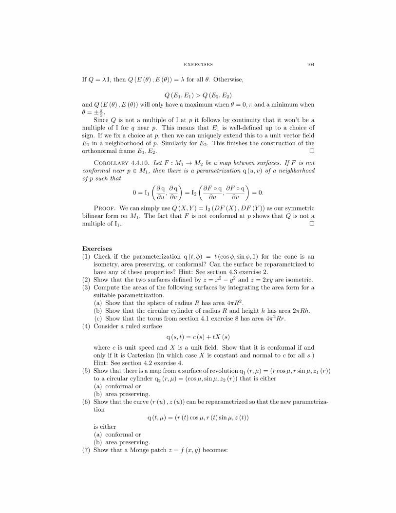
EXERCISES 104
If Q = λ I, then Q (E (θ) , E (θ)) = λ for all θ. Otherwise,
Q (E1, E1) > Q (E2, E2)
and Q (E (θ) , E (θ)) will only have a maximum when θ = 0, π and a minimum whenθ = ±π2 .
Since Q is not a multiple of I at p it follows by continuity that it won’t be amultiple of I for q near p. This means that E1 is well-defined up to a choice ofsign. If we fix a choice at p, then we can uniquely extend this to a unit vector fieldE1 in a neighborhood of p. Similarly for E2. This finishes the construction of theorthonormal frame E1, E2.
Corollary 4.4.10. Let F : M1 →M2 be a map between surfaces. If F is notconformal near p ∈ M1, then there is a parametrization q (u, v) of a neighborhoodof p such that
0 = I1
(∂ q
∂u,∂ q
∂v
)= I2
(∂F q
∂u,∂F q
∂v
)= 0.
Proof. We can simply use Q (X,Y ) = I2 (DF (X) , DF (Y )) as our symmetricbilinear form on M1. The fact that F is not conformal at p shows that Q is not amultiple of I1.
Exercises(1) Check if the parameterization q (t, φ) = t (cosφ, sinφ, 1) for the cone is an
isometry, area preserving, or conformal? Can the surface be reparametrized tohave any of these properties? Hint: See section 4.3 exercise 2.
(2) Show that the two surfaces defined by z = x2 − y2 and z = 2xy are isometric.(3) Compute the areas of the following surfaces by integrating the area form for a
suitable parametrization.(a) Show that the sphere of radius R has area 4πR2.(b) Show that the circular cylinder of radius R and height h has area 2πRh.(c) Show that the torus from section 4.1 exercise 8 has area 4π2Rr.
(4) Consider a ruled surface
q (s, t) = c (s) + tX (s)
where c is unit speed and X is a unit field. Show that it is conformal if andonly if it is Cartesian (in which case X is constant and normal to c for all s.)Hint: See section 4.2 exercise 4.
(5) Show that there is a map from a surface of revolution q1 (r, µ) = (r cosµ, r sinµ, z1 (r))to a circular cylinder q2 (r, µ) = (cosµ, sinµ, z2 (r)) that is either(a) conformal or(b) area preserving.
(6) Show that the curve (r (u) , z (u)) can be reparametrized so that the new parametriza-tion
q (t, µ) = (r (t) cosµ, r (t) sinµ, z (t))
is either(a) conformal or(b) area preserving.
(7) Show that a Monge patch z = f (x, y) becomes:

EXERCISES 105
(a) area preserving if and only if f is constant;(b) conformal if and only if f is constant.
(8) Show that the equationax+ by + cz = d
defines a surface if and only if (a, b, c) 6= (0, 0, 0). Show that this surface has aparametrization that is Cartesian.
(9) The conoid is a special type of ruled surface where c is a straight line and Xalways lies in a fixed plane. The simplest case is when c is the z-axis and Xlies in the (x, y)-plane
q (s, t) = (tx (s) , ty (s) , z (s))
= (0, 0, z (s)) + t (x (s) , y (s) , 0)
(a) Compute its first fundamental form when |X| = 1.(b) Show that this parametrization is conformal (or area preserving) if and
only if the surface is a plane.(c) Show that this surface is a helicoid when both X and z have constant
speed.(d) Show that such a helicoid can be reparametrized using t = t (v) so as to
obtain either a conformal or an area preserving parametrization.(10) Consider the two parametrized surfaces given by
q1 (φ, t) = (sinhφ cos t, sinhφ sin t, t)
= (0, 0, t) + sinhφ (cos t, sin t, 0)
q2 (s, µ) = (cosh s cosµ, cosh s sinµ, s)
Compute the first fundamental forms for both surfaces and construct a localisometry from the first surface to the second. (The first surface is a ruled surfacewith a one-to-one parametrization called the helicoid, the second surface is asurface of revolution called the catenoid.) Hint: See section 4.2 exercise 5.
(11) Consider the tube from section 4.3 exercise 7 with s ∈ [0, L] and φ ∈ [0, 2π].(a) Show that the area is given by 2πRL.(b) Find an area preserving map from this tube to a cylinder of the form
F (q (s, φ)) = (R cosφ,R sinφ, h (s, φ)) .
(12) Consider a generalized cylinder parametrized as in section 4.3 exercise 3 withs ∈ [0, L] and t ∈ [a, b]. Show that its area is L (b− a).
(13) Consider a generalized cone parametrized as in section 4.3 exercise 2 with φ ∈[0, L] and r ∈ [a, b]. Show that its area is 1
2L(b2 − a2
).
(14) Show that Enneper’s surface
q (u, v) =
u− 13u
3 + uv2
v − 13v
3 + vu2
u2 − v2
defines a conformal parametrization.
(15) Show that Catalan’s surface
q (u, v) =
u− sinu cosh v1− cosu cosh v4 sin u
2 sinh v2

EXERCISES 106
defines a conformal parametrization. Hint: Start by showing that: 2 sin2 u2 =
1− cosu etc.(16) Show that the following two parametrizations of the unit sphere are area pre-
serving:(a) (Lambert, 1772)
q (µ, z) =
√1− z2 cosµ√1− z2 sinµ
z
, |µ| < π, |z| < 1.
(b) (Sinusoidal projection, Cossin, 1570)
q (s, t) =
cos s cos(
tcos s
)cos s sin
(t
cos s
)sin s
, |s| < π2 , t < π cos s.
(c) Relate the Lambert parametrization to the Archimedes map.(17) (Stabius-Werner, c. 1500, Sylvanus, 1511, Bonne, c. 1780) Show that the
Bonne parametrizations
q (r, θ) =
cos (r − r0) cos
(r(θ−π/2)cos(r−r0)
)cos (r − r0) sin
(r(θ−π/2)cos(r−r0)
)sin (r − r0)
,have the property that det [I] = r2. Conclude that they are area preservingwhen (r, θ) correspond to polar coordinates
x = r cos θ, y = r sin θ.
For r0 = 0 this is a sinusoidal projection, for r0 = π/2 the Stabius-Wernerprojection, and for 0 < r0 < π/2 the Sylvanus projection. The planar shape ofthese maps is bordered on the outside by an implicitly given curve
|r|∣∣θ − π
2
∣∣ = cos (r − r0)
as r → π/2 this looks like a heart shaped region.(18) Show that the inversion map
F (q) =q
|q|2.
is a conformal map of Rn − 0 to it self. Hint: See section 4.2 exercise 7.(19) Show that the inverse stereographic projections q± : Rn → Rn × R = Rn+1
defined by
q± (q) = (q, 0) +1− |q|2
1 + |q|2(q,±1)
are conformal parametrizations of the unit sphere. Hint: See section 4.2 exercise9. More specifically when n = 2 it is given by
q± (u, v) =
(2u
u2 + v2 + 1,
2v
u2 + v2 + 1,∓u
2 + v2 − 1
u2 + v2 + 1
).

EXERCISES 107
(20) Consider the map F : H → R2 defined by
F (x, y) =1
x2 + (y + 1)2 (2x, 2 (y + 1)) + (0,−1)
=1
x2 + (y + 1)2
(2x, 1− x2 − y2
),
where H = (x, y) | y > 0.(a) Show that F is one-to-one and that the image isD =
(x, y) | x2 + y2 < 1
.
Hint: Show that
|F (x, y)|2 = 1− 4y
x2 + (y + 1)2 .
(b) Show that the inverse is given by
F−1 (u, v) =1
u2 + (v + 1)2 (2u, 2 (v + 1)) + (0,−1)
=1
u2 + (v + 1)2
(2u, 1− u2 − v2
).
(c) Show that F and F−1 are conformal.(d) Show that F can be interpreted as an inversion in the circle of radius
√2
centered at (0,−1).(21) Consider a map F : S2 → P , where P = z = 1 is the plane tangent to the
North Pole, that takes each meridian to the radial line that is tangent to themeridian at the North Pole. Sometimes the map might only be defined on partof the sphere such as the upper hemisphere.(a) Show that such a map has a parametrization of the form
F
cosµ cosφsinµ cosφ
sinφ
=
r (φ) cosµr (φ) sinµ
1
for some function r, where r
(π2
)= 0.
(b) Show that when r =√
2 (1− sinφ), then we obtain an area preserving mapon the upper hemisphere.
(c) Show that when the map projects a point on the upper hemisphere alongthe radial line through the origin, then r = cotφ. Show that this map takesall great circles (not just meridians) to straight lines. This is also calledthe Beltrami projection and is an example of a perspective projection (seesection 4.2 exercise 8).
(d) Show that the inverse of the Beltrami projection from (c) onto the upperhemisphere is given by
B−1 (s, t, 1) =
(s√
1 + s2 + t2,
t√1 + s2 + t2
,1√
1 + s2 + t2
).
(22) Show that a map F : M → M∗ that is both conformal and area preserving isan isometry.
(23) (Girard, 1626) A hemisphere on the unit sphere S2 is the part that lies onone side of a great circle. A lune is the intersection of two hemispheres. Ithas two antipodal vertices. A spherical triangle is the region bounded by threehemispheres.

EXERCISES 108
(a) Show that the area of a hemisphere is 2π.(b) Use the Archimedes map to show that the area of a lune where the great
circles meet at an angle of α is 2α.(c) If A (H) denotes the area of a region on S2 use a Venn type diagram to
show that
A (H1 ∪H2 ∪H3) = A (H1) +A (H2) +A (H3)
−A (H1 ∩H3)−A (H2 ∩H3)−A (H1 ∩H2)
+A (H1 ∩H2 ∩H3) .
(d) Let H1, H2, H3 be hemispheres and H ′i = S2 − Hi the complementaryhemispheres. Show that
H ′1 ∩H ′2 ∩H ′3 = S2 −H1 ∪H2 ∪H3.
And further show that the spherical triangle H1 ∩H2 ∩H3 is congruent tothe spherical triangle H ′1 ∩H ′2 ∩H ′3 via the antipodal map.
(e) Show that the area A of a spherical triangle is given by
A = α+ β + γ − π,where α, β, γ are the interior angles at the vertices of the triangle.

CHAPTER 5
Curvature of Surfaces
The goal of this chapter is to understand curvature of surfaces. This is quite abit more complicated than for curves. There are two curvatures and they are definedas extrinsic invariants, i.e., they depend on how the normal to the surface changes.This is analogous to the curvature of curves. One of the surprising discoveries byGauss was that one of these curvatures is an intrinsic invariant. This means thatit can be calculated knowing only the first fundamental form. Another old problemwe investigate is that of understanding which surfaces admit Cartesian coordinates.
5.1. Curves on Surfaces
In this section the second fundamental form is introduced as the normal partof the acceleration of a curve. This is used to find its matrix representation. Insection 5.2 a more algebraic definition is offered.
We start with the observation that for a surfaceM ⊂ R3 and a point p ∈M thetangent space TpM and normal space NpM = (TpM)
⊥ are defined independentlyof parametrizations (see proposition 4.2.6). Thus the projections of a vector Z ∈ R3
onto both the tangent space and the normal space are well-defined without referenceto parametrizations.
Consider a curve q (t) on the surface. The velocity q and acceleration q can becalculated in R3 without reference to the surface. The velocity will be tangent to thesurface, but the acceleration rarely is. The projections of q onto the normal space,qII = (q · n) n, and the tangent space, qI = q− (q · n) n, can be computed withoutparametrizing the surface. This shows that tangential and normal accelerations arewell-defined.
Theorem 5.1.1 ((Euler, 1760 and Meusnier, 1776)). The normal componentof the acceleration only depends on the surface and the velocity of the curve. Inparticular, two curves with the same velocity at a point have the same normalacceleration components at that point.
Proof. Select a parametrization and write q (t) = q (u (t) , v (t)). Then
q =[∂ q∂u
∂ q∂v
] [ uv
]and
q =
(d
dt
[∂ q∂u
∂ q∂v
]) [ uv
]+[∂ q∂u
∂ q∂v
] [ uv
]=
[u v
] [ ∂2 q∂u2
∂2 q∂u∂v
∂2 q∂v∂u
∂2 q∂v2
] [uv
]+[∂ q∂u
∂ q∂v
] [ uv
].
109
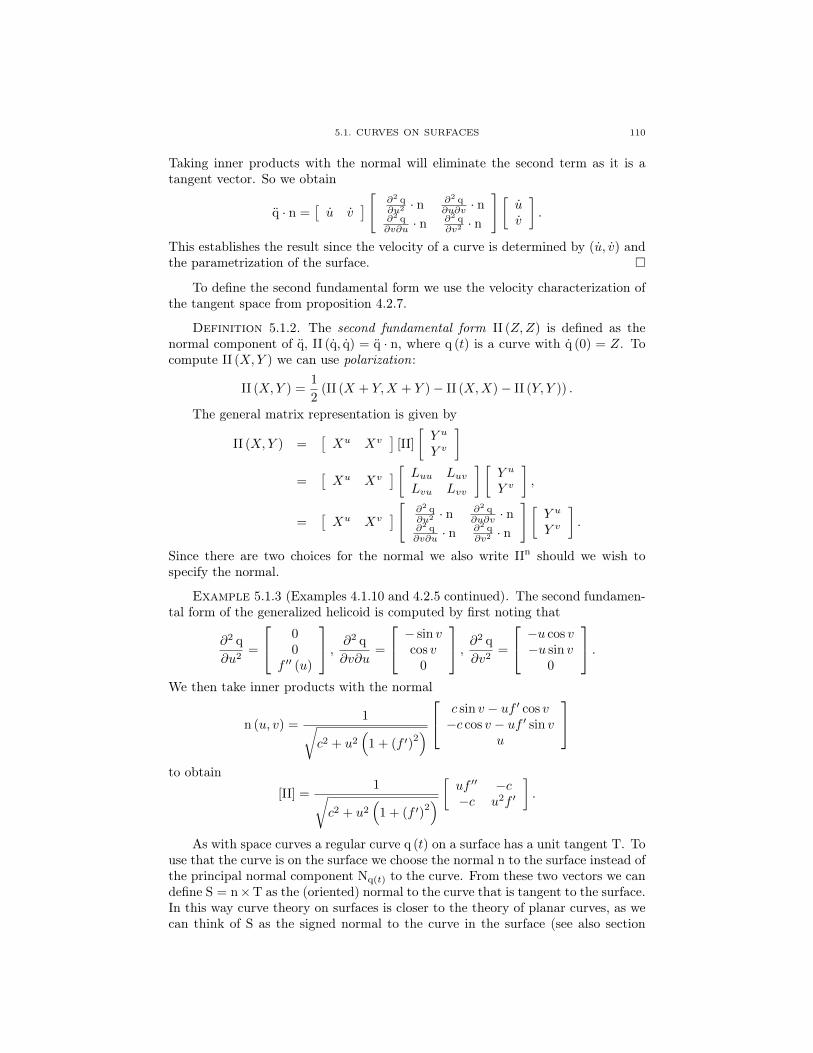
5.1. CURVES ON SURFACES 110
Taking inner products with the normal will eliminate the second term as it is atangent vector. So we obtain
q · n =[u v
] [ ∂2 q∂u2 · n ∂2 q
∂u∂v · n∂2 q∂v∂u · n
∂2 q∂v2 · n
] [uv
].
This establishes the result since the velocity of a curve is determined by (u, v) andthe parametrization of the surface.
To define the second fundamental form we use the velocity characterization ofthe tangent space from proposition 4.2.7.
Definition 5.1.2. The second fundamental form II (Z,Z) is defined as thenormal component of q, II (q, q) = q · n, where q (t) is a curve with q (0) = Z. Tocompute II (X,Y ) we can use polarization:
II (X,Y ) =1
2(II (X + Y,X + Y )− II (X,X)− II (Y, Y )) .
The general matrix representation is given by
II (X,Y ) =[Xu Xv
][II]
[Y u
Y v
]=
[Xu Xv
] [ Luu LuvLvu Lvv
] [Y u
Y v
],
=[Xu Xv
] [ ∂2 q∂u2 · n ∂2 q
∂u∂v · n∂2 q∂v∂u · n
∂2 q∂v2 · n
][Y u
Y v
].
Since there are two choices for the normal we also write IIn should we wish tospecify the normal.
Example 5.1.3 (Examples 4.1.10 and 4.2.5 continued). The second fundamen-tal form of the generalized helicoid is computed by first noting that
∂2 q
∂u2=
00
f ′′ (u)
, ∂2 q
∂v∂u=
− sin vcos v
0
, ∂2 q
∂v2=
−u cos v−u sin v
0
.We then take inner products with the normal
n (u, v) =1√
c2 + u2(
1 + (f ′)2) c sin v − uf ′ cos v−c cos v − uf ′ sin v
u
to obtain
[II] =1√
c2 + u2(
1 + (f ′)2) [ uf ′′ −c
−c u2f ′
].
As with space curves a regular curve q (t) on a surface has a unit tangent T. Touse that the curve is on the surface we choose the normal n to the surface instead ofthe principal normal component Nq(t) to the curve. From these two vectors we candefine S = n×T as the (oriented) normal to the curve that is tangent to the surface.In this way curve theory on surfaces is closer to the theory of planar curves, as wecan think of S as the signed normal to the curve in the surface (see also section

5.1. CURVES ON SURFACES 111
3.3 for the special case of curves on spheres). Using an arclength parameter s wedefine the normal curvature
κn = II (T,T) = n ·dT
ds= −dn
ds· T,
the geodesic curvature
κg = S · dT
ds= −dS
ds· T,
and the geodesic torsion
τg = n ·dS
ds= −dn
ds· S.
Note that the geodesic curvature of curves on the sphere from section 3.3 isconsistent with the above definition.
Example 5.1.4. A plane always has vanishing second fundamental form as itsnormal is constant
II (q, q) = q · n
=d
dt(q · n)− q · n
= −q · n= 0.
This means that any curve in this plane has vanishing normal curvature and geo-desic torsion. The geodesic curvature is the signed curvature κ±.
Example 5.1.5. A sphere of radius R centered at c is given by the equation
F (x, y, z) = |q− c|2 = R2 > 0.
The gradient is∇F = 2 (q− c) = 2 (x− a, y − b, z − c) ,
which cannot vanish unless q = c. This shows that the sphere is a surface and alsocomputes the two normals
n = ± 1
R(q− c) .
as |q− c| = R (see theorem 4.1.9 and corollary 4.2.8). The + gives us an outwardpointing normal. Since n is perpendicular to all tangent vectors this shows that fora curve we have
II (q, q) = q · n
=d
dt(q · n)− q · n
= −q · ddt
(± 1
R(q− c)
)= ∓ 1
Rq · q
= ∓ 1
RI (q, q) .
Thus II = ∓ 1R I and the normal curvature of any curve on the sphere is ∓ 1
R .

5.1. CURVES ON SURFACES 112
Example 5.1.6. We can also relate normal curvature of certain special curvesto the curvature of the curve as follows: For each unit vector X ∈ TpM to a surfacewith normal n consider the plane through p that is spanned by X, n (p). This planehas Y = X × n (p) as a unit normal and intersects the surface in a unit speedcurve q (s) with velocity q = n×Y , i.e., it is the integral curve for n×Y that passesthrough p = q (0) (see section 1.1). Note that at p we have q (0) = X, while atother points it changes with the change in the normal to the surface. The principalnormal as well as the acceleration of this curve at s = 0 must be parallel to n (p)as it is a unit speed curve lies in the plane spanned by X, n. It now follows that
κ (0) = |q (0)| = ±q (0) · n (p) = ±κn (0) = ± II (X,X) .
We shall show below that only planes and spheres have the property thatthe normal curvature is the same for all curves on a surface. Another interestingconsequence is the important theorem, first noted by Euler and later in greatergenerality by Gauss (see theorem 5.3.6), that it is not possible to draws maps ofthe Earth with the property that all distances and angles are preserved.
We start by showing that if a surface admits a Cartesian parametrization, thenthe tangential part of the acceleration is calculated as in the plane.
Proposition 5.1.7. Consider a Cartesian parametrization q (u, v) and a curveq (t) = q (u (t) , v (t)). The tangential and normal components of the accelerationare given by
qI =[∂ q∂u
∂ q∂v
] [ uv
]= u
∂ q
∂u+ v
∂ q
∂v,
qII =[u v
] [ ∂2 q∂u2
∂2 q∂v∂u
∂2 q∂u∂v
∂2 q∂v2
] [uv
]= u2 ∂
2 q
∂u2+ 2uv
∂2 q
∂u∂v+ v2 ∂
2 q
∂v2.
Proof. We saw above that
q =[u v
] [ ∂2 q∂u2
∂2 q∂v∂u
∂2 q∂u∂v
∂2 q∂v2
] [uv
]+[∂ q∂u
∂ q∂v
] [ uv
].
To prove the proposition we need to show that the three vectors ∂2 q∂u2 , ∂2 q
∂v2 , and∂2 q∂v∂u are normal to the surface. This is equivalent to showing that
∂2 q
∂u2· ∂ q
∂w= 0,
∂2 q
∂v∂u· ∂ q
∂w= 0,
∂2 q
∂v2· ∂ q
∂w= 0.
Note that as w = u, v there are 6 identities. Using that ∂ q∂u ,
∂ q∂v are unit vectors we
obtain
0 =∂
∂w
(∂ q
∂u· ∂ q
∂u
)= 2
∂2 q
∂w∂u· ∂ q
∂u=
∂2 q
∂u∂w· ∂ q
∂u
and similarly
0 =∂
∂w
(∂ q
∂v· ∂ q
∂v
)= 2
∂2 q
∂w∂v· ∂ q
∂v=
∂2 q
∂v∂w· ∂ q
∂v.

5.1. CURVES ON SURFACES 113
This shows that four of the identities hold. Next we use that ∂ q∂u ,
∂ q∂v are perpen-
dicular to conclude
0 =∂
∂w
(∂ q
∂u· ∂ q
∂v
)=
∂2 q
∂w∂u· ∂ q
∂v+∂ q
∂u· ∂
2 q
∂w∂v.
Depending on whether w = u or v the second or first term on the right vanishesfrom what we just did. Thus the remaining term also vanishes. This takes care ofthe last two identities.
Theorem 5.1.8 (Euler, 1775). A sphere does not admit a Cartesian parametriza-tion.
Proof. Assume that the surface is a sphere of radius R > 0 centered at theorigin and that part of the sphere admits a Cartesian parametrization q (u, v).Recall that great circles can be characterized as curves with acceleration normalto the sphere, i.e., the tangential acceleration vanishes qI = 0 (see section 3.3exercise 5 or exercise 12 in this section). Thus lines (u (t) , v (t)) in the parameterdomain with vanishing acceleration become parts of great circles q (u (t) , v (t)) onthe sphere. It then simply remains to observe that if we select a small triangle inthe u, v plane, then it is mapped to a congruent spherical triangle whose sides areparts of great circles. This, however, violates the spherical law of cosines as well asGirard’s theorem (see section 4.4 exercise 23). To give a self contained argumenthere, select an equilateral triangle in the plane with side lengths ε. Then we obtainan equilateral triangle on the sphere with side lengths ε and interior angles π
3 . Asthe sides are parts of great circles we can check explicitly if this is possible. Let thevertices be qi, i = 1, 2, 3, then qi · qj = cos ε when i 6= j. The unit directions of thegreat circles at q1 are given by
v12 =q2− (q2 · q1) q1√
1− (q2 · q1)2
=q2− cos ε q1√
1− cos2 ε,
v13 =q3− cos ε q1√
1− cos2 ε
and consequently,
1
2= v12 · v13
=
(q2− cos ε q1√
1− cos2 ε
)·(
q3− cos ε q1√1− cos2 ε
)=
cos ε− 2 cos2 ε+ cos2 ε
1− cos2 ε
=cos ε− cos2 ε
1− cos2 ε
=cos ε
1 + cos ε
<1
2
since cos ε < 1. So we have arrived at a contradiction.

EXERCISES 114
Exercises(1) Show that ∂ n
∂w is always tangent to the surface.(2) Show that
Lw1w2 =∂2 q
∂w1∂w2· n = − ∂ q
∂w2· ∂ n
∂w1.
This shows that the derivatives of the normal can be computed knowing thefirst and second fundamental forms.
(3) Show that the unit normal is constant if and only if the surface is part of aplane.
(4) Show that [II] vanishes if and only if the normal vector is constant. (Hint: useexercise (2))
(5) Consider a parametrized surface q (u, v).(a) Show that ∂2 q
∂u∂v is normal to the surface if and only if ∂guu∂v = ∂gvv∂u = 0.
(b) Show that ∂2 q∂u2 is normal to the surface when ∂guu
∂u = ∂guu∂v = ∂guv
∂u = 0.(c) Show that ∂2 q
∂u2 + ∂2 q∂v2 is normal to the surface when guu = gvv and guv = 0.
(6) A curve q (t) on a surface is called an asymptotic curve if II (q, q) = 0, i.e., κnvanishes.(a) Show that a curve is asymptotic if and only if its acceleration is tangent to
the surface.(b) Show that the binormal to an asymptotic curve is normal to the surface.
(7) Let c (s) be a unit speed curve with non-vanishing curvature. Show that c isan asymptotic curve on the ruled surface
q (s, t) = c (s) + tNc (s) ,
where Nc is the principal normal to c as a space curve.(8) Let q (s) be a unit speed curve on a surface with normal n. Show that κg = 0
if and only ifdet [q, q,n] = 0.
(9) Consider the parabolic surface z = x2
a2 + y2
b2 where a, b > 0.(a) Show that q (t) =
(at cos θ, bt sin θ, t2
)is a regular curve on this surface.
(b) Show that when a = b (surface of revolution), then κg = 0 for all θ.(c) Show that when a 6= b, then κg = 0 if and only if sin 2θ = 0.
(10) Show that latitudes on a sphere have constant κg.(11) Let q (s) be a unit speed curve on a surface and let n be the normal to the
surface. Show that
d
ds
[T S n
]=[
T S n] 0 −κg −κn
κg 0 −τgκn τg 0
.(12) For a curve on the unit sphere (see also exercise (1) in section 3.3) show that
(a) τg = 0.(b) κg = 0 if and only if it is a great circle.(c) κg is constant if and only if it is a circle.
(13) Let q (t) be a regular curve on a surface with n being the normal to the surface.Show that
κn =II (q, q)
I (q, q), κg =
det (q, q,n)
(I (q, q))3/2
.

EXERCISES 115
(14) Let q (u, v) be a parametrization such that guu = 1 and guv = 0. Prove that theu-curves are unit speed with acceleration that is perpendicular to the surface.Hint: The u-curves are given by q (u) = q (u, v) where v is fixed.
(15) Consider a surface of revolution
q (s, θ) = (r (s) cos (θ) , r (s) sin (θ) , z (s)) ,
where, r > 0, z > 0, and (r (s) , 0, z (s)) is unit speed.(a) Compute the second fundamental form.(b) Compute κg, κn, τg for the meridians q (s) = q (s, θ). Conclude that their
acceleration is perpendicular to the surface(c) Compute κg, κn, τg for the latitudes q (θ) = q (s, θ). Hint: The latitudes
are not necessarily unit speed, but they do have constant speed.(16) Let M be a surface with normal n and X,Y ∈ TpM . Show that if q (t) is a
curve with velocity X at t = 0 and Y (t) is an extension of the vector Y to avector field along q, then
II (X,Y ) = n ·dYdt
(0) .
(17) Let q (s) be a unit speed curve on a surface with normal n. Show that the spacecurvature κ is related to the geodesic and normal curvatures as follows
κ2 = κ2g + κ2
n
and that the torsion is given by
τ = τg +κgκn − κnκgκ2g + κ2
n
.
Hint: Start by showing that
q = κgS + κn n,...q = −
(κ2g + κ2
n
)T + (κg − κnτg) S + (κn + κgτg) n .
(18) Let M be a surface given by an equation F (x, y, z) = R.(a) If q (t) is a curve on M show that
q · ∇F = −qt
∂2F∂x2
∂2F∂x∂y
∂2F∂x∂z
∂2F∂y∂x
∂2F∂y2
∂2F∂y∂z
∂2F∂z∂x
∂2F∂z∂y
∂2F∂z2
q
= −qt[
∂∇F∂ (x, y, z)
]q.
(b) Show that
II (X,Y ) = −Xt[
∂∇F∂(x,y,z)
]Y
|∇F |.
(19) Assume that a unit speed curve q (s) = q (u (s) , v (s)) on a parametrized surfacesatisfies an equation F (u, v) = R.(a) If we use ∂wF = ∂F
∂w show that u∂uF + v∂vF = 0.

5.2. THE GAUSS AND WEINGARTEN MAPS AND EQUATIONS 116
(b) Show that
q = u∂ q
∂u+ v
∂ q
∂v
=±1√
guu∂vF∂vF − 2guv∂uF∂vF + gvv∂uF∂uF
(−∂vF
∂ q
∂u+ ∂uF
∂ q
∂v
).
This means that the unit tangent can be calculated without reference tothe parametrization of the curve.
(c) Show that if we use this formula for the velocity, then the geodesic curvaturecan be computed as
κg =
∂∂u
(q · ∂ q
∂v
)− ∂
∂v
(q · ∂ q
∂u
)√
det [I].
(d) Generalize this to the situation where a unit speed curve satisfies a differ-ential relation
Pu+Qv = 0,
where P = P (u, v) and Q = Q (u, v).
5.2. The Gauss and Weingarten Maps and Equations
In the last section we calculated the normal part of the acceleration of a curve.To gain a better understanding of the tangential component we need to furtheranalyze the second partial derivatives of a parametrized surface. We use proposition4.3.5 to decompose these derivatives in to tangential and normal components
∂2 q
∂w1∂w2=[∂ q∂u
∂ q∂v
][I]−1 [ ∂ q
∂u∂ q∂v
]t ∂2 q
∂w1∂w2+
(∂2 q
∂w1∂w2· n)
n,
where w1, w2 can be either u or v. In the previous section the normal componentwas identified as an entry in the matrix representation of the second fundamentalform. The tangential part is denoted by
Γw1w2 =[∂ q∂u
∂ q∂v
][I]−1 [ ∂ q
∂u∂ q∂v
]t ∂2 q
∂w1∂w2.
Definition 5.2.1. The Christoffel symbols of the first kind are defined as
Γw1w2w =∂2 q
∂w1∂w2· ∂ q
∂w,[
Γw1w2u Γw1w2v
]=
[∂ q∂u ·
∂2 q∂w1∂w2
∂ q∂v ·
∂2 q∂w1∂w2
]=
[∂ q∂u
∂ q∂v
]t ∂2 q
∂w1∂w2
and the Christoffel symbols of the second kind are defined as
Γww1w2= gwuΓw1w2u + gwvΓw1w2v,[
Γuw1w2
Γvw1w2
]=
[guu guv
gvu gvv
] [Γw1w2u
Γw1w2v
]= [I]
−1 [ ∂ q∂u
∂ q∂v
]t ∂2 q
∂w1∂w2,
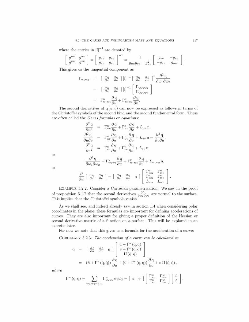
5.2. THE GAUSS AND WEINGARTEN MAPS AND EQUATIONS 117
where the entries in [I]−1 are denoted by[
guu guv
gvu gvv
]=
[guu guvgvu gvv
]−1
=1
guugvv − g2uv
[gvv −guv−gvu guu
].
This gives us the tangential component as
Γw1w2=
[∂ q∂u
∂ q∂v
][I]−1 [ ∂ q
∂u∂ q∂v
]t ∂2 q
∂w1∂w2
=[∂ q∂u
∂ q∂v
][I]−1
[Γw1w2u
Γw1w2v
]= Γuw1w2
∂ q
∂u+ Γvw1w2
∂ q
∂v.
The second derivatives of q (u, v) can now be expressed as follows in terms ofthe Christoffel symbols of the second kind and the second fundamental form. Theseare often called the Gauss formulas or equations:
∂2 q
∂u2= Γuuu
∂ q
∂u+ Γvuu
∂ q
∂v+ Luu n,
∂2 q
∂u∂v= Γuuv
∂ q
∂u+ Γvuv
∂ q
∂v+ Luv n =
∂2 q
∂v∂u,
∂2 q
∂v2= Γuvv
∂ q
∂u+ Γvvv
∂ q
∂v+ Lvv n,
or∂2 q
∂w1∂w2= Γuw1w2
∂ q
∂u+ Γvw1w2
∂ q
∂v+ Lw1w2
n,
or∂
∂w
[∂ q∂u
∂ q∂v
]=[∂ q∂u
∂ q∂v n
] Γuwu ΓuwvΓvwu ΓvwvLwu Lwv
.Example 5.2.2. Consider a Cartesian parametrization. We saw in the proof
of proposition 5.1.7 that the second derivatives ∂2 q∂w1∂w2
are normal to the surface.This implies that the Christoffel symbols vanish.
As we shall see, and indeed already saw in section 1.4 when considering polarcoordinates in the plane, these formulas are important for defining accelerations ofcurves. They are also important for giving a proper definition of the Hessian orsecond derivative matrix of a function on a surface. This will be explored in anexercise later.
For now we note that this gives us a formula for the acceleration of a curve:
Corollary 5.2.3. The acceleration of a curve can be calculated as
q =[∂ q∂u
∂ q∂v n
] u+ Γu (q, q)v + Γv (q, q)
II (q, q)
= (u+ Γu (q, q))
∂ q
∂u+ (v + Γv (q, q))
∂ q
∂v+ n II (q, q) ,
where
Γw (q, q) =∑
w1,w2=u,v
Γww1w2w1w2 =
[u v
] [ Γwuu ΓwuvΓwvu Γwvv
] [uv
].

5.2. THE GAUSS AND WEINGARTEN MAPS AND EQUATIONS 118
Proof. This follows directly from
q =[u v
] [ ∂2 q∂u2
∂2 q∂u∂v
∂2 q∂v∂u
∂2 q∂v2
] [uv
]+[∂ q∂u
∂ q∂v
] [ uv
]and the Gauss formulas above.
Note that the tangential component is quite complicated[∂ q∂u
∂ q∂v
][I]−1 [ ∂ q
∂u∂ q∂v
]tq = qI =
∂ q
∂u(u+ Γu (q, q)) +
∂ q
∂v(v + Γv (q, q)) .
But it seems to be a more genuine acceleration as it includes second derivatives. Ittells us what acceleration we feel on the surface.
To complete the Gauss formulas it is natural to also include the derivatives ofthe normal vector.
Definition 5.2.4. The Gauss map for an orientable surface M with normaln is the map n : M → S2 (1) that takes each point to the chosen normal at thatpoint. The Weingarten map at a point p ∈ M is the linear map L : TpM → TpMdefined as the negative of the differential of n:
L = −D n .
Remark 5.2.5. The definition of the Weingarten map requires some explana-tion as the differential should be a linear map
D n : TpM → Tn(p)S2 (1) .
However, the normal vector to any point x ∈ S2 (1) is simply n = ±x. As thetangent space is the orthogonal complement to the normal vector it follows that
TpM = Tn(p)S2 (1) .
For a parametrized surface this tells us.
Proposition 5.2.6 (The Weingarten Equations). For a parametrized surfaceq (u, v) we have
−∂ n
∂u= L
(∂ q
∂u
),
−∂ n
∂v= L
(∂ q
∂v
).
More generally, for a curve q (t) on the surface
−dn q
dt= L
(d q
dt
).
Proof. The equations simply follow from the chain rule and the first two arespecial cases of the last. If we write the curve q (t) = q (u (t) , v (t)), then
L
(d q
dt
)= −D n
(d q
dt
)= −dn q
dt
= −(∂ n
∂u
du
dt+∂ n
∂v
dv
dt
).
This proves the claim
5.2. THE GAUSS AND WEINGARTEN MAPS AND EQUATIONS 119
Next we show that the Weingarten map L is a self-adjoint map with respect tothe first fundamental form.
Proposition 5.2.7. The Weingarten map is abstractly related to the secondfundamental form through the first fundamental form by the formula:
I (L (X) , Y ) = II (X,Y ) = I (X,L (Y ))
In particular, L is self-adjoint as II is symmetric.
Proof. Since the second fundamental form is symmetric II (X,Y ) = II (Y,X),it follows that we only need to show that I (L (X) , Y ) = II (X,Y ), as we have
I (X,L (Y )) = I (L (Y ) , X)
= II (Y,X)
= II (X,Y ) .
Next observe that since L is linear it suffices to prove that
II
(∂ q
∂w1,∂ q
∂w2
)= I
(L
(∂ q
∂w1
),∂ q
∂w2
)for all choices w1, w2 ∈ u, v where q (u, v) is a parametrization. Using that ∂ q
∂w2
and n are perpendicular it follows that
0 =∂
∂w1
(∂ q
∂w2· n)
=∂2 q
∂w1∂w2· n +
∂ q
∂w2· ∂ n q
∂w1
= II
(∂ q
∂w1,∂ q
∂w2
)− ∂ q
∂w2· L(∂ q
∂w1
)= II
(∂ q
∂w1,∂ q
∂w2
)− I
(L
(∂ q
∂w1
),∂ q
∂w2
).
This proves the claim.
All in all this is still a bit abstract, but the relationship between the Weingartenmap and the first and second fundamental forms allow us to obtain explicit formulasfor a parametrized surface.
Given a parametrized surface q (u, v) the entries in the matrix representationof the Weingarten map are defined as[
L(∂ q∂u
)L(∂ q∂v
) ]=
[∂ q∂u
∂ q∂v
][L]
=[∂ q∂u
∂ q∂v
] [ Luu LuvLvu Lvv
].
This matrix representation can be calculated as follows.
Proposition 5.2.8. The matrix representations of the Weingarten map andthe second fundamental form satisfy:
[L] = [I]−1
[II]

5.2. THE GAUSS AND WEINGARTEN MAPS AND EQUATIONS 120
and
[II] = −[∂ n∂u
∂ n∂v
]t [ ∂ q∂u
∂ q∂v
]= −
[∂ n∂u ·
∂ q∂u
∂ n∂u ·
∂ q∂v
∂ n∂v ·
∂ q∂u
∂ n∂v ·
∂ q∂v
]= −
[∂ q∂u
∂ q∂v
]t [ ∂ n∂u
∂ n∂v
].
Proof. To establish the formula for [II] use that n is perpendicular to ∂ q∂w2
and note that
Lw1w2=
∂2 q
∂w1∂w2· n
=
(∂
∂w1
(∂ q
∂w2
))· n
=∂
∂w1
(∂ q
∂w2· n)− ∂ q
∂w2· ∂ n
∂w1
= − ∂ q
∂w2· ∂ n
∂w1.
It now follows that
[II] =[∂ q∂u
∂ q∂v
]t [ −∂ n∂u −∂ n
∂v
]=
[∂ q∂u
∂ q∂v
]t [L(∂ q∂u
)L(∂ q∂v
) ]=
[∂ q∂u
∂ q∂v
]t [ ∂ q∂u
∂ q∂v
][L]
= [I] [L] .
Remark 5.2.9. It is important to realize that while L is self-adjoint its matrixrepresentation
[L] = [I]−1
[II]
need not be symmetric. In fact, as [I] and [II] are symmetric it follows that
[L]t
= [II] [I]−1.
So [L] is only symmetric if [I] and [II] commute.
The Weingarten equations are the formulas for the derivatives of the normal:∂ n
∂w= −Luw
∂ q
∂u− Lvw
∂ q
∂v= −L
(∂ q
∂w
).
Together the Gauss formulas and Weingarten equations tell us how the deriva-tives of our basis ∂ q
∂u ,∂ q∂v ,n relate back to the basis. They can be collected as
follows:
Corollary 5.2.10 (The Gauss and Weingarten Formulas).∂
∂w
[∂ q∂u
∂ q∂v n
]=
[∂ q∂u
∂ q∂v n
][Dw]
=[∂ q∂u
∂ q∂v n
] Γuwu Γuwv −LuwΓvwu Γvwv −LvwLwu Lwv 0
.

5.2. THE GAUSS AND WEINGARTEN MAPS AND EQUATIONS 121
Finally we show how the Christoffel symbols can be calculated directly fromthe first fundamental form without knowing the second derivatives ∂2 q
∂w1∂w2.
Proposition 5.2.11. The Christoffel symbols of the first kind satisfy
Γuuu =1
2
∂guu∂u
,
Γuvu =1
2
∂guu∂v
= Γvuu,
Γvvv =1
2
∂gvv∂v
,
Γuvv =1
2
∂gvv∂u
= Γvuv,
Γuuv =∂guv∂u− 1
2
∂guu∂v
,
Γvvu =∂guv∂v− 1
2
∂gvv∂u
.
Proof. We prove only two of these as the proofs are all similar. First use theproduct rule to see
Γuvu =∂2 q
∂u∂v· ∂ q
∂u=
(∂
∂v
(∂ q
∂u
))· ∂ q
∂u=
1
2
∂
∂v
(∂ q
∂u· ∂ q
∂u
)=
1
2
∂guu∂v
.
Now use this together with the product rule to find
Γuuv =∂2 q
∂u∂u· ∂ q
∂v
=
(∂
∂u
(∂ q
∂u
))· ∂ q
∂v
=∂
∂u
(∂ q
∂u· ∂ q
∂v
)−(∂ q
∂u· ∂
2 q
∂u∂v
)=
∂guv∂u− ∂ q
∂u· ∂
2 q
∂v∂u
=∂guv∂u− 1
2
∂guu∂v
.
Example 5.2.12. While these formulas for the Christoffel symbols can’t bemade simpler as such, it is possible to be a bit more efficient in several concretesituations. Specifically, we often do calculations in orthogonal coordinates, i.e.,guv ≡ 0. In such coordinates
guv = 0,
guu = (guu)−1,
gvv = (gvv)−1,

EXERCISES 122
Γuuu =1
2
∂guu∂u
,
Γuvu =1
2
∂guu∂v
= Γvuu,
Γvvv =1
2
∂gvv∂v
,
Γuvv =1
2
∂gvv∂u
= Γvuv,
Γuuv = −1
2
∂guu∂v
,
Γvvu = −1
2
∂gvv∂u
,
and
Γuuu =1
2guu
∂guu∂u
=1
2
1
guu
∂guu∂u
=∂ ln√guu
∂u,
Γvuu = −1
2gvv
∂guu∂v
= −1
2
1
gvv
∂guu∂v
,
Γvvv =1
2gvv
∂gvv∂v
=1
2
1
gvv
∂gvv∂v
=∂ ln√gvv
∂v,
Γuvv = −1
2guu
∂gvv∂u
= −1
2
1
guu
∂gvv∂u
,
Γuuv =1
2guu
∂guu∂v
=1
2
1
guu
∂guu∂v
=∂ ln√guu
∂v,
Γvuv =1
2gvv
∂gvv∂u
=1
2
1
gvv
∂gvv∂u
=∂ ln√gvv
∂u.
Often there might be even more specific information. This could be that themetric coefficients only depend on one of the parameters, or that guu = 1. In suchcircumstances it is quite manageable to calculate the Christoffel symbols. What ismore, we show in proposition 7.4.1 that it is always possible to find parametrizationswhere guu ≡ 1 and guv ≡ 0. In this case:
Γuuu = Γvuu = Γuuv = Γuvu = Γuuu = Γuuv = Γuvu = Γvuu = 0.
Example 5.2.13. Consider a Cartesian parametrization. We saw in the proofof proposition 5.1.7 that the second derivatives ∂2 q
∂w1∂w2are normal to the surface.
This fact now also follows from the fact that the Christoffel symbols vanish.
Exercises(1) For a surface of revolution
q (t, θ) = (r (t) cos (θ) , r (t) sin (θ) , z (t))
compute the first and second fundamental forms and the Weingarten map.(2) Compute the matrix representation of the Weingarten map for a Monge patch
q (x, y) = (x, y, f (x, y)) with respect to the basis ∂ q∂x ,
∂ q∂y .
(3) Show that if a surface satisfies II = ± 1R I, then it is part of a sphere of radius
R. Hint: Show that n± 1R q is constant and use that to find the center of the
sphere.

EXERCISES 123
(4) Let M be a surface with normal n and X,Y ∈ TpM . Show that if q (t) is acurve with velocity X at t = 0 , then
II (X,Y ) = −Y · dn q
dt(0) .
(5) Show that for a curve on a surface the geodesic torsion satisfies
τg = II (T,S) .
(6) Show that guu, guv, and gvv are constant if and only if the Christoffel symbolsof the first kind vanish.
(7) Show that∂gw1w2
∂w= Γww1w2
+ Γww2w1
and use these equations to show that
2Γw1w2w =∂gww2
∂w1+∂gww1
∂w2− ∂gw1w2
∂w.
(8) Show thatΓw1w2w = gwuΓuw1w2
+ gwvΓvw1w2
.
(9) Show that∂ det [I]
∂w=
2
det [I](Γuwu + Γvwv) ,
∂√
det [I]
∂w=√
det [I] (Γuwu + Γvwv) ,
and∂ log
√det [I]
∂w= Γuwu + Γvwv.
(10) Let θ be the angle between ∂ q∂u and ∂ q
∂v . Show that
log sin θ = log√
det [I]− 1
2log guu −
1
2log gvv,
cot θ =guv√det [I]
,
and∂θ
∂w= −
√det [I]
guuΓvwu −
√det [I]
gvvΓuwv.
(11) Show that
I (Γw1w2,Γw3w4
) =[
Γuw1w2Γvw1w2
][I]
[Γuw3w4
Γvw3w4
]=
[Γw1w2u Γw1w2v
] [ Γuw3w4
Γvw3w4
]=
[Γw1w2u Γw1w2v
][I]−1
[Γw3w4u
Γw3w4v
].

EXERCISES 124
(12) Show directly from the formulas for the Christoffel symbols in terms of the firstfundamental form that
∂
∂vΓuuv −
∂
∂uΓuvv =
∂
∂uΓvvu −
∂
∂vΓuvu
and∂
∂vΓuuv −
∂
∂uΓuvv = −1
2
∂2guu∂v2
+∂2guv∂u∂v
− 1
2
∂2gvv∂u2
.
(13) (Surface of revolution) Find the Christoffel symbols of the first and second kindwhen the first fundamental form is given by
[I] =
[1 00 r2
],
where r = r (u) > 0.(14) (Polar and Fermi coordinates) Find the Christoffel symbols of the first and
second kind when the first fundamental form is given by
[I] =
[1 00 r2
],
where r = r (u, v) > 0. Gauss showed that such coordinates exist around anypoint in a surface with r denoting the “intrinsic” distance to the point. Fermicreated such coordinates in a neighborhood of a geodesic with r denoting the“intrinsic” distance to the geodesic. The terminology will be explained later.
(15) Find the Christoffel symbols of the first and second kind when the first funda-mental form is given by
[I] =
[r2 00 r2
],
where r = r (u) > 0.(16) (Isothermal coordinates) Find the Christoffel symbols of the first and second
kind when the first fundamental form is given by
[I] =
[r2 00 r2
],
where r = r (u, v) > 0.(17) (Liouville surfaces) Find the Christoffel symbols of the first and second kind
when the first fundamental form is given by
[I] =
[r2 00 r2
],
where r2 = f (u) + g (v) > 0.(18) (Monge patch) Find the Christoffel symbols of the first and second kind when
the first fundamental form is given by
[I] =
[1 + p2 pqpq 1 + q2
],
where p = ∂F∂u , q = ∂F
∂v and F = F (u, v).

5.3. THE GAUSS AND MEAN CURVATURES 125
5.3. The Gauss and Mean Curvatures
We are now finally ready to define the curvatures of a surface. Historically theprincipal curvatures defined in section 5.4 came first, but it seems equally naturalto start with the Gauss and mean curvatures.
Definition 5.3.1. The Gauss curvature is defined as the determinant of theWeingarten map
K = detL.
The mean curvature is related to the trace as follows
H =1
2trL.
To calculate these quantities we have:
Proposition 5.3.2. The Gauss and mean curvatures of a parametrized surfaceq (u, v) can be computed as
K =det [II]
det [I]=LuuLvv − (Luv)
2
guugvv − (guv)2
andH =
1
2
gvvLuu + guuLvv − 2guvLuv
guugvv − (guv)2 .
Proof. To calculate the Gauss and mean curvatures we use the formulas fordeterminant and trace of a matrix representation:
K = det [L] = LuuLvv − LvuLuv ,
H =1
2tr [L] =
1
2(Luu + Lvv) ,
and [L] = [I]−1
[II] (see proposition 5.2.8). The formula for K now follows fromstandard determinant rules.
For H we use that
Luu = guuLuu + guvLvu and Lvv = gvuLuv + gvvLvv
together with [guu guv
gvu gvv
]=
1
det [I]
[gvv −guv−gvu guu
]to get the desired formula.
Example 5.3.3. For a sphere of radius R we have that II = ± 1R I. Thus
K = 1R2 and H = ± 1
R . For a plane II = 0 and K = H = 0.
Example 5.3.4 (Examples 4.3.3 and 5.1.3 continued). We can now calculatethe Gauss and mean curvatures of the generalized helicoids
K =det [II]
det [I]=
u3f ′f ′′ − c2(c2 + u2
(1 + (f ′)
2))2 ,
H =1
2
(1 + (f ′)
2)u2f ′ +
(u2 + c2
)uf ′′ + 2c2f ′(
c2 + u2(
1 + (f ′)2)) 3
2
.

5.3. THE GAUSS AND MEAN CURVATURES 126
Remark 5.3.5. It is often convenient to calculate the mean curvature usingthe formula
H =1
2
(gvv
∂2 q∂u2 + guu
∂2 q∂v2 − 2guv
∂2 q∂u∂v
)· n
guugvv − (guv)2 ,
which follows directly from the above proposition and the definition of the entriesin the second fundamental form.
We can now significantly improve theorem 5.1.8 as was first done by Gauss.This result is also a corollary of the next theorem.
Theorem 5.3.6 (Gauss). If a surface in R3 admits Cartesian coordinates, thenthe Gauss curvature vanishes.
Proof. We saw in the proof of proposition 5.1.7 that when a parametrizationof a surface q (u, v) is Cartesian, then the second derivatives ∂2 q
∂u∂v ,∂2 q∂u2 , and ∂2 q
∂v2
are all normal to the surface. This shows with explanations below that
det [II] =
(∂2 q
∂u2· n)(
∂2 q
∂v2· n)−(∂2 q
∂u∂v· n)2
=∂2 q
∂u2· ∂
2 q
∂v2− ∂2 q
∂u∂v· ∂
2 q
∂u∂v
=∂2 q
∂u2· ∂
2 q
∂v2+
∂3 q
∂u2∂v· ∂ q
∂v
=∂2 q
∂u2· ∂
2 q
∂v2+
∂3 q
∂v∂u2· ∂ q
∂v
=∂2 q
∂u2· ∂
2 q
∂v2− ∂2 q
∂u2· ∂
2 q
∂v2
= 0,
where lines 3 and 5 follow from
0 =∂
∂u
(∂2 q
∂u∂v· ∂ q
∂v
)=
∂3 q
∂u2∂v· ∂ q
∂v+
∂2 q
∂u∂v· ∂
2 q
∂u∂v
and
0 =∂
∂v
(∂2 q
∂u2· ∂ q
∂v
)=
∂3 q
∂v∂u2· ∂ q
∂v+∂2 q
∂u2· ∂
2 q
∂v2.
This shows that the Gauss curvature vanishes.
The converse is also true and is covered in section 6.3 exercise 9 and theorem7.7.1. Section 5.5 contains a more detailed discussion of what surfaces with zeroGauss curvature look like.
Remark 5.3.7. Given that planes, generalized cylinders, and generalized conesall admit Cartesian coordinates it is easy to come up with examples showing thatthe mean curvature cannot be calculated from the first fundamental form. In factonly planes have the property that the Gauss and mean curvatures both vanish.
We can use our knowledge of Christoffel symbols to improve the theorem forCartesian coordinates to the general result that the Gauss curvature can alwaysbe computed from the first fundamental form. Given the definition of K this iscertainly a big surprise.

5.3. THE GAUSS AND MEAN CURVATURES 127
Theorem 5.3.8 (Theorema Egregium, Gauss, 1827 ). The Gauss curvature canbe computed knowing only the first fundamental form.
Proof. Assume that we have a parametrized surface q (u, v). The calculationsare similar to what we just did for a Cartesian parametrization. First we observethat it suffices to show that det [II] can be calculated from the first fundamentalform since
K = detL = det [I]−1
det [II] ,
det [I] = guugvv − (guv)2.
We use the Gauss formulas to compute
det [II] = det
[Luu LuvLvu Lvv
]= det
[∂2 q∂u2 · n ∂2 q
∂u∂v · n∂2 q∂v∂u · n
∂2 q∂v2 · n
]
=
(∂2 q
∂u2· n)(
∂2 q
∂v2· n)−(∂2 q
∂u∂v· n)(
∂2 q
∂u∂v· n)
=∂2 q
∂u2· ∂
2 q
∂v2−(
Γuuu∂ q
∂u+ Γvuu
∂ q
∂v
)·(
Γuvv∂ q
∂u+ Γvvv
∂ q
∂v
)− ∂2 q
∂u∂v· ∂
2 q
∂u∂v+
∣∣∣∣Γuuv ∂ q
∂u+ Γvuv
∂ q
∂v
∣∣∣∣2Here the inner products(
Γuuu∂ q
∂u+ Γvuu
∂ q
∂v
)·(
Γuvv∂ q
∂u+ Γvvv
∂ q
∂v
)and ∣∣∣∣Γuuv ∂ q
∂u+ Γvuv
∂ q
∂v
∣∣∣∣2can be calculated from the first fundamental form as we proved in proposition 5.2.11that the inner products
Γw1w2w =∂ q
∂w· ∂2 q
∂w1∂w2
have formulas that only use the derivatives of guu, guv, and gvv (see also section5.2 exercise 11).
To finish the proof it simply remains to observe that
∂2 q
∂u2· ∂
2 q
∂v2− ∂2 q
∂u∂v· ∂
2 q
∂u∂v
=∂
∂v
(∂2 q
∂u2· ∂ q
∂v
)− ∂3 q
∂v∂u2· ∂ q
∂v
− ∂
∂u
(∂2 q
∂u∂v· ∂ q
∂v
)+
∂3 q
∂2u∂v· ∂ q
∂v
=∂
∂vΓuuv −
∂
∂uΓvuv.
(See also section 5.2 exercise 12 for a nice formula of this combination of derivatives.)The complete formula for the Gauss curvature in terms of the first fundamental

5.3. THE GAUSS AND MEAN CURVATURES 128
form and the Christoffel symbols of the first kind is given in exercise 13 to thissection.
Example 5.3.9. Assume that guu = 1 and guv = 0 as in the end of example5.2.12. In this case the above proof reduces the Gauss curvature to:
K =1
gvv
(− ∂
∂uΓvuv + (Γvuv)
2gvv
)=
1
gvv
(−1
2
∂2gvv∂u2
+
(1
gvv
1
2
∂gvv∂u
)2
gvv
)
= −1
2
1
gvv
∂2gvv∂u2
+1
4
(1
gvv
∂gvv∂u
)2
= − 1√gvv
∂2√gvv∂u2
.
The Gauss curvature can also be expressed more directly in terms of the unitnormal.
Proposition 5.3.10 (Gauss). The Gauss curvature satisfies
K =
(∂ n∂u ×
∂ n∂v
)· n(
∂ q∂u ×
∂ q∂v
)· n.
Proof. Simply use the Weingarten equations to calculate∂ n
∂u× ∂ n
∂v=
(−Luu
∂ q
∂u− Lvu
∂ q
∂v
)×(−Luv
∂ q
∂u− Lvv
∂ q
∂v
)= LuuL
vv
∂ q
∂u× ∂ q
∂v+ LvuL
uv
∂ q
∂v× ∂ q
∂u
= (LuuLvv − LvuLuv )
∂ q
∂u× ∂ q
∂v
= K∂ q
∂u× ∂ q
∂v.
Note that the denominator in
K =
(∂ n∂u ×
∂ n∂v
)· n(
∂ q∂u ×
∂ q∂v
)· n
is already computed in terms of the first fundamental form((∂ q
∂u× ∂ q
∂v
)· n)2
=
∣∣∣∣∂ q
∂u× ∂ q
∂v
∣∣∣∣2 = guugvv − (guv)2.
The numerator is the signed volume of the parallelepiped ∂ n∂u ,
∂ n∂v ,n corresponding
to the Gauss map n (u, v) : U → S2 (1) ⊂ R3 of the surface. Thus it can becomputed from the first fundamental form of n (u, v). However, there is a sign thatdepends on whether n and ∂ n
∂u ×∂ n∂v point in the same direction or not. Recall
from curve theory that the tangent spherical image was also related to curvaturein a similar way. Here the formulas are a bit more complicated as we use arbitraryparameters.

5.3. THE GAUSS AND MEAN CURVATURES 129
Definition 5.3.11. The third fundamental form III on TpM is defined as thefirst fundamental form for S2 (1) on Tn(p)S
2 (1). If we use the Gauss map n (u, v) =n q (u, v) as the parametrization, then the matrix representation is given by
[III] =[∂ n∂u
∂ n∂v
]t [ ∂ n∂u
∂ n∂v
]=
[∂ n∂u ·
∂ n∂u
∂ n∂u ·
∂ n∂v
∂ n∂v ·
∂ n∂u
∂ n∂v ·
∂ n∂v
].
This always defines a quadratic from, but n might not be a genuine parametriza-tion if the Gauss curvature vanishes. Nevertheless, we alway have the relationship
∂ n
∂u× ∂ n
∂v= K
(∂ q
∂u× ∂ q
∂v
).
The three fundamental forms and two curvatures are related by a very interest-ing formula which also shows that the third fundamental form is almost redundant.
Theorem 5.3.12. All three fundamental forms are related by
III−2H II +K I = 0.
Proof. We prove this for the matrix representations
[III]− 2H [II] +K [I] = 0
by reducing it to the Cayley-Hamilton theorem for [L]
[L]2 − (trL) [L] + (detL) I2 = 0,
where I2 is the 2 × 2 identity matrix. This relies on showing: [I] [L] = [II] and[I] [L]
2= [III]. The first identity has already been established. The second likewise
follows from the Weingarten equations:
[III] =[L(∂ q∂u
)L(∂ q∂v
) ]t [L(∂ q∂u
)L(∂ q∂v
) ]= [L]
t [ ∂ q∂u
∂ q∂v
]t [ ∂ q∂u
∂ q∂v
][L]
= [L]t[I] [L]
= [II]t(
[I]−1)t
[I] [L]
= [II] [I]−1
[I] [L]
= [II] [L]
= [I] [L] [L]
= [I] [L]2.

5.3. THE GAUSS AND MEAN CURVATURES 130
Finally, if [L] =
[a cb d
], then the Cayley-Hamilton theorem follows by a direct
calculation:
[L]2 − (trL) [L] + (detL) I2
=
[a cb d
]2
− (a+ d)
[a cb d
]+ (ad− bc)
[1 00 1
]=
[a2 + bc ac+ dcab+ db bc+ d2
]− (a+ d)
[a cb d
]+ (ad− bc)
[1 00 1
]=
[bc− ad 0
0 bc− ad
]+ (ad− bc)
[1 00 1
]= 0.
Definition 5.3.13. A surface is called minimal if its mean curvature vanishes.
Proposition 5.3.14. A minimal surface has conformal Gauss map.
Proof. Let q (u, v) be a parametrization of the surface, then n (u, v) is a poten-tial parametrization of the unit sphere via the Gauss map. The first fundamentalform with respect to this parametrization is the third fundamental form. UsingH = 0 we obtain
[III] +K [I] = 0,
which implies that the Gauss map is conformal.
Example 5.3.15. Note that the Gauss map for the unit sphere centered at theorigin is simply the identity map on the sphere. Thus its Gauss map is an isometryand in particular conformal. However, the sphere is not a minimal surface. Moregenerally, the Gauss map
n (q) = ±q− c
R
for a sphere of radius R centered at c is also conformal as its derivative is given byD n = ± 1
RI, where I is the identity map/matrix.
The name for minimal surfaces is justified by the next result. Meusnier in1785 was the first to consider such surfaces and he also indicated with a geometricargument that their areas should be minimal. In fact Lagrange in 1761 had alreadycome up with an (Euler-Lagrange) equation for surfaces that minimize area, butit was not until the mid 19th century with Bonnet and Beltrami that this wasdefinitively connected to the condition that the mean curvature should vanish.
Example 5.3.16 (Example 5.3.4 continued). We note that the generalized he-licoids are minimal when f ′ = 0, i.e., when they are regular helicoids. In the rota-tionally symmetric case where c = 0, they are minimal when f = a cosh−1
(ua
)+ b,
for constants a, b. These are all catenoids.Finally, we also obtain a more complicated family by using
f ′ =c
u
√u2 + c2
u2 − c2.

5.3. THE GAUSS AND MEAN CURVATURES 131
To see this first note that
1 + (f ′)2
=u4 + c4
u2 (u2 − c2), f ′′ = −f ′
(1
u+
2c2u
(u2 − c2) (u2 + c2)
).
The numerator in the formula for H then becomes
u4 + c4
u2 (u2 − c2)u2f ′ −
(u2 + c2
)uf ′
(1
u+
2c2u
(u2 − c2) (u2 + c2)
)+ 2c2f ′
after eliminating f ′ and multiplying through by u2 − c2 this expression becomes
u4 + c4 −(u4 − c4 + 2c2u2
)+ 2c2
(u2 − c2
)= 0.
Theorem 5.3.17. A surface whose area is minimal among nearby surfaces isa minimal surface.
Proof. We assume that the surface is given by a parametrization q (u, v) andonly consider nearby surfaces that are graphs over the given surface, i.e.,
q∗ = q +φn
for some function φ (u, v). From such a surface we can then create a family ofsurfaces
qε = q +εφn
that interpolates between these two surfaces. To calculate the area density as afunction of ε we first note that
∂ qε∂w
=∂ q
∂w+ ε
(∂φ
∂wn +φ
∂ n
∂w
).
Then the first fundamental form becomes
gεww = gww + 2εφ∂ q
∂w· ∂ n
∂w+ ε2
((∂φ
∂w
)2
+ φ2
∣∣∣∣∂ n
∂w
∣∣∣∣2)
= gww − 2εφLww + ε2
((∂φ
∂w
)2
−Kφ2gww + 2Hφ2Lww
),
gεuv = guv + εφ
(∂ q
∂u· ∂ n
∂v+∂ q
∂v· ∂ n
∂u
)+ ε2
(∂φ
∂u· ∂φ∂v
+ φ2 ∂ n
∂u· ∂ n
∂v
)= guv − 2εφLuv + ε2
(∂φ
∂u· ∂φ∂v−Kφ2guv + 2Hφ2Luv
),
and the square of the area density
gεuugεvv − (gεuv)
2= guugvv − (guv)
2 − 2ε (guuLvv + gvvLuu − 2guvLuv) +O(ε2)
=(guugvv − (guv)
2)
(1− 4εφH) +O(ε2).
This shows that if H 6= 0 somewhere then we can select φ such that the areadensity will decrease for nearby surfaces.

EXERCISES 132
Remark 5.3.18. Conversely note that when H = 0 everywhere, then the areadensity is critical. The term that involves ε2 has a coefficient that looks like
guu
((∂φ
∂v
)2
− φ2Kgvv
)+ gvv
((∂φ
∂u
)2
− φ2Kguu
)
−2guv
(∂φ
∂u· ∂φ∂v− φ2Kguv
)+ 4φ2
(LuuLvv − L2
uv
)=
∣∣∣∣−∂φ∂v ∂ q
∂u+∂ q
∂v
∂φ
∂u
∣∣∣∣2 − 2φ2K(guugvv − g2
uv
)+ 4φ2
(LuuLvv − L2
uv
)=
∣∣∣∣−∂φ∂v ∂ q
∂u+∂ q
∂v
∂φ
∂u
∣∣∣∣2 + 2φ2K(guugvv − g2
uv
)and it is not clear that this is positive. In fact, minimal surfaces have K ≤ 0 sowhen φ is constant the area decreases!
Exercises(1) Let X,Y ∈ TpM be an orthonormal basis for the tangent space at p to the
surface M . Prove that the mean and Gauss curvatures can be computed asfollows:
H =1
2(II (X,X) + II (Y, Y )) ,
K = II (X,X) II (Y, Y )− (II (X,Y ))2.
(2) Show that ifK = 0 and H = 0, then the Weingarten map L = 0 and the normalis constant. Hint: First show that the third fundamental form vanishes. Givean example of a 2× 2 matrix A 6= 0 such that A2 = 0 and trA = 0 = detA.
(3) Assume that K = H = 0 and use the equations
LuuLvv − (Luv)2
= 0,
gvvLuu + guuLvv − 2guvLuv = 0,
to show that II = 0. Hint: First show that if Luv = 0, then Luu = Lvv = 0.Second, if Luv 6= 0, then use guugvv > (guv)
2 and LuuLvv = (Luv)2 to show
that the last equation can’t be satisfied.(4) Show that if K = 1
R2 and H = ± 1R , then the Weingarten map L = ∓ 1
RI, whereI is the identity operator. Use this to show that the surface is part of a sphereon radius R.
(5) For a surface of revolution
q (t, µ) = (r (t) cosµ, r (t) sinµ, z (t))
compute the first and second fundamental forms as well as the Gauss and meancurvatures. Show that if (r (t) , z (t)) is unit speed, then K = − rr .
(6) Compute the second fundamental form of a tangent developable q (s, t) = c (t)+sdcdt of a unit speed curve c (t). Show that the Gauss curvature vanishes. Showthat the mean curvature vanishes if and only if the second fundamental formvanishes.

EXERCISES 133
(7) Show that the surface of revolution
q (s, θ) =
(R cos (as) cos θ,R cos (as) sin θ,
∫ s
0
√1− a2R2 sin2 (at)dt
)has constant Gauss curvature a2. Show that this is a sphere centered at theorigin if and only if R = 1
a . Hint: When s = 0 this is a circle of radius R.(8) Show that a Monge patch z = F (x, y) is minimal if and only if Lagrange’s
equation holds:(1 +
(∂F
∂y
)2)∂2F
∂x2− 2
∂F
∂x
∂F
∂y
∂2F
∂x∂y+
(1 +
(∂F
∂x
)2)∂2F
∂y2= 0.
Use this to show that Scherk’s surface ecz cos cx = cos cy is minimal. In factScherk’s surface is the only minimal surface of the form z = F (x, y) = f (x) +h (y).
(9) Let q (t) be a curve on a surface with normal n. Denote the Gauss image of thecurve by n (t) = n q (t). Show that the velocities of these curves are relatedby ∣∣∣∣dn
dt
∣∣∣∣2 + 2Hdn
dt· d q
dt+K
∣∣∣∣d q
dt
∣∣∣∣2 = 0.
(10) Let q (t) = q (u (t) , v (t)) be an asymptotic curve on a surface, i.e., κn = 0.(a) Show that K ≤ 0 along the curve.(b) (Beltrami-Enneper) If τ is the torsion of the curve as a space curve, then
τ2 = −K.
Hint: Use the previous exercise.(11) Show that a minimal surface satisfies K ≤ 0.(12) Show that if a parametrized surface has the property that guu, gvv, and guv are
constant, then the second derivatives ∂2 q∂u∂v ,
∂2 q∂u2 , and ∂2 q
∂v2 are all normal to thesurface. Use this to conclude that the Gauss curvature vanishes.
(13) Show that
K =1
det [I]
(∂
∂vΓuuv −
∂
∂uΓuvv
)− 1
det [I]
[Γuuu Γuuv
][I]−1
[ΓvvuΓvvv
]+
1
det [I]
[Γuvu Γuvv
][I]−1
[ΓuvuΓuvv
].
Hint: See section 5.2 exercise 11.(14) Compute the Gauss curvatures of the generalized cones (section 4.1 exercise 2),
generalized cylinders (section 4.1 exercise 1), and tangent developables (section4.1 exercise 3). We shall offer several proofs below that these are essentially theonly surfaces with vanishing Gauss curvature (see 29 below and section 5.5).Hint: In each case the normal vector is constant along the lines in the ruledsurface.
(15) Show that∂ q
∂u× ∂ n
∂v+∂ n
∂u× ∂ q
∂v= −2H
∂ q
∂u× ∂ q
∂v,

EXERCISES 134
and more generally that
∂ q
∂u× ∂ n
∂w= −Lvw
∂ q
∂u× ∂ q
∂v,
∂ n
∂w× ∂ q
∂v= −Luw
∂ q
∂u× ∂ q
∂v.
(16) Show that
2K√
det [I] n =∂
∂u
(n× ∂ n
∂v
)− ∂
∂v
(n× ∂ n
∂u
),√
det [I] n×∂ n
∂u= Luv
∂ q
∂u− Luu
∂ q
∂v,√
det [I] n×∂ n
∂v= Lvv
∂ q
∂u− Luv
∂ q
∂v.
Hint: For the last two formulas it might be useful to use section 4.3 exercise 9and [II] = [I] [L].
(17) Compute the first and second fundamental forms as well as the Gauss and meancurvatures for the conoid
q (s, t) = (sx (t) , sy (t) , z (t))
= (0, 0, z (t)) + s (x (t) , y (t) , 0)
when X = (x (t) , y (t) , 0) is a unit field.(18) Show that a conformally parametrized (isothermal) surface q (u, v) is minimal
if and only if
∆ q =∂2 q
∂u2+∂2 q
∂v2= 0.
Hint: Use section 5.1 exercise 5c.(19) Show that Enneper’s surface
q (u, v) =
(u− 1
3u3 + uv2, v − 1
3v3 + vu2, u2 − v2
)is minimal. Hint: Do section 4.4 exercise 14 first.
(20) Show that Catalan’s surface
q (u, v) =(u− sinu cosh v, 1− cosu cosh v,−4 sin
u
2sinh
v
2
)is minimal. Hint: Do section 4.4 exercise 15 first.
(21) Show that for a fixed θ ∈ R the parametrized surface
q (u, v) = (u cos θ ± sinu cosh v, v ± cos θ cosu sinh v,± sin θ cosu cosh v)
is isothermal and minimal.(22) Consider a unit speed curve c (s) : [0, L] → R3 with non-vanishing curvature
and the tube of radius R around it
q (s, φ) = c (s) +R (Nc cosφ+ Bc sinφ)
(see section 4.1 exercise 6 and section 4.3 exercise 7).(a) Use the formula for n together with Gauss’ formula for K to show that
K =−κ cosφ
R (1− κR cosφ).
EXERCISES 135
(b) Show that ∫ 2π
0
∫ L
0
K√
det [I]dsdφ = 0
and ∫ 2π
0
∫ L
0
|K|√
det [I]dsdφ = 4
∫ L
0
κds.
(23) Consider a surface with negative Gauss curvature.(a) Show that locally it admits a parametrization q (s, t) where the parameter
curves are asymptotic curves, i.e., the second fundamental form looks like
[II] =
[0 LstLst 0
].
(b) Show that this implies
[III] = −K[
gss −gst−gst gtt
].
(24) (Meusnier, 1785) Consider a surface of revolution of the form
q (t, µ) = (r (t) cosµ, r (t) sinµ, t) .
(a) Show that if the surface of revolution is minimal thenr
r2 + 1=
1
r.
(b) Show that the catenoids
q (t, µ) =
(1
acosh (at+ b) cosµ,
1
acosh (at+ b) sinµ, t
),
a > 0 and b ∈ R are minimal.(c) Show that the functions
r (t) =1
acosh (at+ b)
solve the initial value problems:r
r2 + 1=
1
r, r (0) = r0 > 0, r (0) = r0 ∈ R.
(d) Conclude that the catenoids are the only surfaces of revolution that areminimal.
(25) (Meusnier, 1785) Show that the helicoid
q (r, θ) = (r cos θ, r sin θ, θ)
is minimal. Conversely, show that if a conoid
q (r, θ) = (r cos θ, r sin θ, z (θ))
is minimal, then z = aθ + b, for constants a, b.(26) Consider a parametrized surface q (u, v) with normal n (u, v) and let f (u, v) be
a function.(a) Show that
K =det(∂(f n)∂u , ∂(f n)
∂v , f n)
f2 det(∂ q∂u ,
∂ q∂v , f n
) .

EXERCISES 136
(b) Show that
H = −1
2
det(∂ q∂u ,
∂(f n)∂v , f n
)+ det
(∂(f n)∂u , ∂ q
∂v , f n)
f det(∂ q∂u ,
∂ q∂v , f n
) .
Hint: When f = 1 this follows from 15.(c) Show that if the surface satisfies F (x, y, z) = C, then there is a function f
such that ∇F = f n.(27) Consider a surface that satisfies the equation F (x, y, z) = C and use n = ∇F
|∇F | .(In section 2.1 exercise 13 there is a similar problem for planar curves given byequations.)(a) Assume that ∂F
∂z 6= 0 and use x, y as parameters for a Monge patch. Showthat
∂ q
∂x=
1∂F∂z
∂F∂z0−∂F∂x
, ∂ q
∂y=
1∂F∂z
0∂F∂z
−∂F∂y
and
∂∇F∂x
=
∂2F∂x2
∂2F∂x∂y∂2F∂x∂z
− ∂F∂x∂F∂z
∂2F∂z∂x∂2F∂z∂y∂2F∂z2
, ∂∇F∂y
=
∂2F∂y∂x∂2F∂y2
∂2F∂y∂z
− ∂F∂y
∂F∂z
∂2F∂z∂x∂2F∂z∂y∂2F∂z2
.Hint: Keep in mind that z = z (x, y) and that its derivatives can be calcu-lated using implicit differentiation.
(b) Use (a) and exercise 26 to show that
K = − 1
|∇F |4det
∂2F∂x2
∂2F∂y∂x
∂2F∂z∂x
∂F∂x
∂2F∂x∂y
∂2F∂y2
∂2F∂z∂y
∂F∂y
∂2F∂x∂z
∂2F∂y∂z
∂2F∂z2
∂F∂z
∂F∂x
∂F∂y
∂F∂z 0
.Hint: Use a Laplace expansion along the bottom row.
(c) Why is the formula in (b) valid at all points where ∇F 6= 0?(d) Show that the surfaces
x2
a2+y2
b2+z2
c2= 1,
x2
a2+y2
b2− z2
c2= −1
haveK =
1
a2b2c21(
x2
a4 + y2
b4 + z2
c4
)2 .
(e) Show that the surface
x2
a2+y2
b2− z2
c2= 1
hasK = − 1
a2b2c21(
x2
a4 + y2
b4 + z2
c4
)2 .
EXERCISES 137
(f) Show that the surface
x2
a2+y2
b2= z,
hasK =
1
4a2b21(
x2
a4 + y2
b4 + 14
)2 .
(g) Show that the surfacex2
a2− y2
b2= z
hasK = − 1
4a2b21(
x2
a4 + y2
b4 + 14
)2 .
(28) Consider a surface that satisfies the equation F (x, y, z) = C and use n =∇F|∇F | . (In section 2.1 exercise 14 a similar problem for planar curves given byequations.)(a) Assume that ∂F
∂z 6= 0 and use x, y as parameters for a Monge patch. Showthat
∂ q
∂x=
1∂F∂z
∂F∂z0−∂F∂x
, ∂ q
∂y=
1∂F∂z
0∂F∂z
−∂F∂y
and
∂∇F∂x
=
∂2F∂x2
∂2F∂x∂y∂2F∂x∂z
− ∂F∂x∂F∂z
∂2F∂z∂x∂2F∂z∂y∂2F∂z2
, ∂∇F∂y
=
∂2F∂y∂x∂2F∂y2
∂2F∂y∂z
− ∂F∂y
∂F∂z
∂2F∂z∂x∂2F∂z∂y∂2F∂z2
.Hint: Keep in mind that z = z (x, y) and that its derivatives can be calcu-lated using implicit differentiation.
(b) Using part (a) and exercise 26 show that
H = −1
2div∇F|∇F |
,
where
div
PQR
=∂P
∂x+∂Q
∂y+∂R
∂z.
Hint: It might help to first show that
div∇F|∇F |
=∆F
|∇F |− (∇F )
tD2F∇F|∇F |3
,
where
∆F =∂2F
∂x2+∂2F
∂y2+∂2F
∂z2
and
(∇F )tD2F∇F =
[∂F∂x
∂F∂y
∂F∂z
]∂2F∂x2
∂2F∂y∂x
∂2F∂z∂x
∂2F∂x∂y
∂2F∂y2
∂2F∂z∂y
∂2F∂x∂z
∂2F∂y∂z
∂2F∂z2
∂F
∂x∂F∂y∂F∂z
.

EXERCISES 138
(c) Show that Scherk’s surface ez cosx = cos y is minimal.(d) Show that sin az = sinh ax sinh ay defines a minimal surface.(e) Can you find other minimal surfaces of the form F (x)G (y)H (z) = 1?
(29) (Monge 1775) Consider a Monge patch z = F (x, y). Define the two functionsp = ∂F
∂x and q = ∂F∂y .
(a) Show that the Gauss curvature vanishes if and only if
∂2F
∂x2
∂2F
∂y2−(∂2F
∂x∂y
)2
= 0.
(b) Assume that ∂2F∂x∂y = 0 on an open set.
(i) Show that F = f (x) + h (y).(ii) Show that the Gauss curvature vanishes if and only if f ′′ = 0 or
h′′ = 0.(iii) Show that if, say, h′′ = 0, then it is a generalized cylinder.
(c) Assume that ∂2F∂x∂y 6= 0 and that the Gauss curvature vanishes.
(i) Show that we can locally reparametrize the surface using the reparametriza-tion (u, q) = (x, q (x, y)).
(ii) Show that p = f (q) for some function f . Hint: In the (u, q)-coordinates ∂p
∂u = 0. When doing this calculation keep in mind thaty depends on u in (u, q)-coordinates as q depends on both x and y.
(iii) Show in the same way that F (x, y)− (px+ qy) = h (q).(iv) Show that in the new parametrization:
y = −h′ (q)− uf ′ (q)
and
z = xp+ qy + h (q)
= h (q)− qh′ (q) + (f (q)− qf ′ (q))u.
(v) Show that this is a ruled surface.(vi) Show that this ruled surface is a generalized cylinder when f ′′ van-
ishes.(vii) Show that it is a generalized cone when h′′ = af ′′ for some constant
a.(viii) Show that otherwise it is a tangent developable by showing that the
lines in the ruling are all tangent to the curve that corresponds to
u = −h′′
f ′′.

5.4. PRINCIPAL CURVATURES 139
(30) Show that
K =
det
∂2 q∂u2 ·
(∂ q∂u ×
∂ q∂v
)∂2 q∂u∂v ·
(∂ q∂u ×
∂ q∂v
)∂2 q∂v∂u ·
(∂ q∂u ×
∂ q∂v
)∂2 q∂v2 ·
(∂ q∂u ×
∂ q∂v
) (det [I])
2
=
(∂∂vΓuuv − ∂
∂uΓuvv)
det [I]
+
det
0 Γvvu ΓvvvΓuuu guu guvΓuuv gvu gvv
− det
0 Γuvu ΓuvvΓuvu guu guvΓuvv gvu gvv
(det [I])
2 .
(31) (Gauss) Show that if we define |g|2 = det [I], then
4 |g|4K = guu
(∂guu∂v
∂gvv∂v− 2
∂guv∂u
∂gvv∂v
+
(∂gvv∂u
)2)
+guv
(∂guu∂u
∂gvv∂v− ∂gvv
∂u
∂guu∂v− 2
∂guu∂v
∂guv∂v− 2
∂gvv∂u
∂guv∂u
+ 4∂guv∂u
∂guv∂v
)+gvv
(∂guu∂u
∂gvv∂u− 2
∂guu∂u
∂guv∂v
+
(∂guu∂v
)2)
−2 |g|2(∂2guu∂v2
− 2∂2guv∂u∂v
+∂2gvv∂u2
).
(32) (Frobenius) Show that if we define |g|2 = det [I], then
K = − 1
4 |g|2det
guu guv gvv∂guu∂u
∂guv∂u
∂gvv∂u
∂guu∂v
∂guv∂v
∂gvv∂v
− 1
2 |g|
(∂
∂u
(∂gvv∂u −
∂guv∂v
|g|
)+
∂
∂v
(∂guu∂v −
∂guv∂u
|g|
)).
(33) (Liouville) Show that if we define |g|2 = det [I], then
K =1
|g|
(∂
∂v
(|g|guu
Γvuu
)− ∂
∂u
(|g|guu
Γvuv
))=
1
|g|
(∂
∂v
(|g|gvv
Γuvv
)+
∂
∂u
(|g|gvv
Γuuv
)).
5.4. Principal Curvatures
Definition 5.4.1. The principal curvatures at a point q on a surface are
κ1 = max II (X,X) | X ∈ TqM and |X| = 1 ,κ2 = min II (X,X) | X ∈ TqM and |X| = 1 .
We say that q is umbilic if the principal curvatures coincide, i.e., II is a multiple ofI at q.

5.4. PRINCIPAL CURVATURES 140
Theorem 5.4.2 (Euler, 1760). Let E ∈ TqM be a unit vector and κ1, κ2 theprincipal curvatures, then
II (E,E) = κ1 cos2 θ + κ2 sin2 θ.
Moreover, the principal curvatures are eigenvalues for the Weingarten map.
Proof. We argue as in the proof of theorem 4.4.9 with Q = II. Let II (E,E)have a maximum at E1 with E2 ∈ TqM a unit vector orthogonal to E1. It followsthat all unit vectors at q have the form E (θ) = cos θE1 + sin θE2 ∈ TqM . Nowconsider
II (E (θ) , E (θ)) = cos2 θ II (E1, E1) + 2 cos θ sin θ II (E1, E2) + sin2 θ II (E2, E2) .
By construction this is a function of θ that has a maximum at θ = 0. The derivativeat θ = 0 is 2 II (E1, E2). Therefore, II (E1, E2) = 0 and
II (E (θ) , E (θ)) = cos2 θ II (E1, E1) + sin2 θ II (E2, E2) .
We claim that L (Ei) = κiEi for i = 1, 2. To see this note that
L (E1) = I (L (E1) , E1)E1 + I (L (E1) , E2)E2
= II (E1, E1)E1 + II (E1, E2)E2
= κ1E1.
A similar argument works for E2.
Definition 5.4.3. A vector that is an eigenvector for the Weingarten map iscalled a principal direction. A curve on a surface with the property that its velocityis always an eigenvector for the Weingarten map, i.e., a principal direction, is calleda line of curvature.
By using II = Q in theorem 4.4.9 we obtain:
Corollary 5.4.4. If a point q on a surface is not umbilic, then there is aparametrization q (u, v) such that the coordinate curves are lines of curvature:
L
(∂ q
∂u
)= κ1
∂ q
∂u, L
(∂ q
∂v
)= κ2
∂ q
∂v,
andI
(∂ q
∂u,∂ q
∂v
)= Q
(∂ q
∂u,∂ q
∂v
)= 0.
Example 5.4.5. The height function that measures the distance from a pointon the surface to the tangent space TqM is given by
f (q) = (q−q) · n (q) .
Its partial derivatives with respect to a parametrization of the surface are∂f
∂w=
∂ q
∂w· n (q) ,
∂2f
∂w1∂w2=
∂2 q
∂w1∂w2· n (q) .
Thus f has a critical point at q, and the second derivative matrix at q is simply [II] .The second derivative test then tells us something about how the surface is placedin relation to TqM. Specifically we see that if both principal curvatures have thesame sign, or K > 0, then the surface must locally be on one side of the tangent

5.4. PRINCIPAL CURVATURES 141
plane, while if the principal curvatures have opposite signs, or K < 0, then thesurface lies on both sides. In that case it’ll look like a saddle.
We can now give a rather surprising characterization of planes and spheres.
Theorem 5.4.6 (Meusnier, 1776). If a surface has the property that κ1 = κ2
at all points, then κ1 = κ2 = H is constant and the surface is part of a plane orsphere.
Proof. Since the principal curvatures are the eigenvalues of L it follows thatH = κ1+κ2
2 = κ1 = κ2.Assume we have a parametrization q (u, v) of part of the surface. Since the
principal curvatures agree at all points it follows that all directions are principaldirections. In particular:
−∂ n
∂w= L
(∂ q
∂w
)= H
∂ q
∂w.
By letting w = u, v and taking partial derivatives of this equation we obtain
− ∂2 n
∂u∂v=
∂H
∂u
∂ q
∂v+H
∂2 q
∂u∂v,
− ∂2 n
∂v∂u=
∂H
∂v
∂ q
∂u+H
∂2 q
∂v∂u.
As partial derivatives commute it follows that
∂H
∂u
∂ q
∂v=∂H
∂v
∂ q
∂u.
Since ∂ q∂u ,
∂ q∂v are linearly independent this forces ∂H
∂u = ∂H∂v = 0. Thus H is
constant.Returning to the equation
−∂ n
∂w= H
∂ q
∂w
we see that∂ (n +H q)
∂w= 0.
This implies that n +H q is constant. When H = 0 this shows that n is constantand consequently the surface lies in a plane orthogonal to n. When H does notvanish we can assume that H = ± 1
R , R > 0. We then have that
±R n + q = c
for some c ∈ R3. This shows that
|q− c|2 = R2.
Hence q lies on the sphere of radius R centered at c.

EXERCISES 142
Exercises(1) Show that if two nonzero tangent vectors X,Y to a surface satisfy I (X,Y ) =
0 = II (X,Y ), then they are principal directions.(2) Show that the principal curvatures for a parametrized surface are the roots to
the equationdet ([II]− κ [I]) = 0.
(3) Show that the principal curvatures are given by
κ1 = H +√H2 −K and κ2 = H −
√H2 −K.
(4) Show that if H ≤ H0 and K ≥ K0, then κ1 ≤ H0 +√H2
0 −K0 and κ2 ≥H0 −
√H2
0 −K0.(5) Show that following conditions are equivalent:
(a) The principal curvatures at a point are equal.(b) The mean and Gauss curvatures at the point are related by H2 = K.(c) L = HI, where I is the identity map on the tangent spaces.(d) (L−HI)
2= 0.
(e) The characteristic polynomial for L is a perfect square.(6) Let q (u, v) be a parametrized surface without umbilics. Show that ∂ q
∂u and ∂ q∂v
are the principal directions if and only if guv = 0 = Luv.(7) Consider
z(x2 + y2
)= κ1x
2 + κ2y2.
(a) Show that this defines a surface when x2 + y2 > 0.(b) Show that it is a ruled surface where the lines go through the z-axis and
are perpendicular to the z-axis.(c) Show that if a general surface has principal curvatures κ1, κ2 at a point,
then z corresponds to the possible values of the normal curvature at thatpoint.
(8) (Rodrigues) Show that a curve q (t) on a surface with normal n is a line ofcurvature if and only if there is a function λ (t) such that
−λ (t)d q
dt=d (n q)
dt.
(9) Show that the principal curvatures are constant if and only if the Gauss andmean curvatures are constant.
(10) Consider the pseudo-sphere
q (t, µ) =
(cosµ
cosh t,
sinµ
cosh t, t− tanh t
).
This is a model for a surface with constant negative Gauss curvature. Notethat the surface
q (t, µ) =
(cosµ
cosh t,
sinµ
cosh t, tanh t
)is the sphere with a conformal (Mercator) parametrization.(a) Compute the first and second fundamental forms(b) Compute the principal curvatures, Gauss curvature, and mean curvature.
(11) A ruled surface q (u, v) = c (v)+uX (v) is called developable if all of the u-curvesq (u) = q (u, v) for fixed v are lines of curvature with κ = 0, i.e., ∂ n
∂u = 0. Showthat ruled surfaces are developable if and only if they have vanishing Gausscurvature.

EXERCISES 143
(12) (Monge) Show that a curve q (t) on a surface with normal n is a line of curvatureif and only if the ruled surface q∗ (s, t) = q (t) + sn q (t) is developable. Hint:Note that the normal to q∗ (s, t) = q (t) + sn q (t) at s = 0 is S (t). So thissurface is developable if and only if S (t0) is the normal to q∗ (s, t0) for all s.
(13) Show that if a surface has conformal Gauss map, then it is either minimal orpart of a sphere.
(14) Show that if III = λ II for some function λ on the surface, then either K = 0or the surface is part of a sphere.
(15) Show that all curves on a sphere or plane are lines of curvature. Use this toshow that if two spheres; a plane and a sphere; or two planes intersect in acurve, then they intersect at a constant angle along this curve.
(16) Consider a surface of revolution
q (r, µ) = (r cosµ, r sinµ, h (r)) .
Show that κ1 = ddr (rκ2).
(17) Consider a unit speed curve c (s) : [0, L] → R3 with non-vanishing curvatureand the tube of radius R around it
q (s, φ) = c (s) +R (Nc cosφ+ Bc sinφ)
(see section 4.1 exercise 6 and section 4.3 exercise 7). Show that the principaldirections are −Nc sinφ + Bc cosφ and Tc with principal curvatures 1/R and− κ cosφ
1−κR cosφ .(18) Show that Enneper’s surface
q (u, v) =
(u− 1
3u3 + uv2, v − 1
3v3 + vu2, u2 − v2
)has the property that guv = Luv = 0 and that the u- and v-curves are planar.Hint: A curve is planar if det
[v a j
]= 0.
(19) Show that
q (u, v) = (u cos θ ± sinu cosh v, v ± cos θ cosu sinh v,± sin θ cosu cosh v)
has the property that guv = Luv = 0 and that the u- and v-curves are planar.Hint: A curve is planar if det
[v a j
]= 0.
(20) Consider a parametrized surface q (t, φ) where the t- and φ-curves correspondto the principal directions. Assume that the principal curvatures are κ2 < κ1
and κ1 = 1/R is constant.(a) Consider c (t, φ) = q (t, φ) +R n (t, φ) and show that
∂ c
∂φ= 0,
∂ c
∂t6= 0.
(b) Conclude that q is a tube of radius R (see section 4.1 exercise 6).(c) Show that a surface without umbilics where one of the principal curvatures
is a positive constant is a tube.(d) Is it necessary to assume that the surface has no umbilics?
(21) Show that the geodesic torsion of a curve on a surface satisfies
τg = (κ2 − κ1) sinφ cosφ,
where φ is the angle between the tangent to the curve and the principal directioncorresponding to κ1.

EXERCISES 144
(22) (Rodrigues) Show that a unit speed curve on a surface is a line of curvature ifand only if its geodesic torsion vanishes.
(23) (Joachimsthal) Let q (t) be a curve that lies on two surfaces M1 and M2 thathave normals n1 and n2 respectively. Define
θ (t) = ∠ (n1 q (t) ,n2 q (t))
and assume that 0 < θ (t) < π, in other words the surfaces are not tangent toeach other along the curve.(a) Show that if q (t) is a line of curvature on both surfaces, then θ (t) is
constant.(b) Show that if q (t) is a line of curvature on one of the surfaces and θ (t) is
constant, then q (t) is also a line of curvature on the other surface.(24) Let q (u, v) be a parametrized surface and qR = q +R n the parallel surface at
distance R from q.(a) Show that
∂ qR
∂w=∂ q
∂w+R
∂ n
∂w= (I −RL)
(∂ q
∂w
),
where I is the identity map I (v) = v.(b) Show that qR is a parametrized surface with normal n provided R 6= 1
κ1, 1κ2.
(c) Show thatLR = L (I −RL)
−1
by using that
L
(∂ q
∂w
)= −∂ n
∂w= LR
(∂ qR
∂w
).
(d) Show that these surfaces all have the same principal directions with prin-cipal curvatures
κRi =κi
1−Rκi.
(25) Let q (u, v) be a parametrized surface and qR = q +R n the parallel surface atdistance ε from q.(a) Show that
IR = I−2R II +R2 III .
(b) Show thatIIR = II−R III .
(c) Show thatIIIR = III .
(d) How do you reconcile these relations with the formula
LR = L (I −RL)−1
from the previous exercise?(e) Show that
KR =K
1− 2RH +R2Kand
HR =H −RK
1− 2RH +R2K.

5.5. RULED SURFACES 145
(f) Show that if K = 1R2 , then H±R = 1
2R . Conversely, if H = 12R , then
KR = 1R2 .
(g) Show that
det[IR]
=(1− 2RH +R2K
)2det [I] .
5.5. Ruled Surfaces
A ruled surface comes about by selecting a curve c (v) and then considering thesurface one obtains by adding a line through each of the points on the curve. If thedirections of those lines are given by X (v), then the surface can be parametrizedby q (u, v) = c (v) + uX (v). We can without loss of generality assume that X is aunit field, however, in many concrete examples throughout the exercises X mightnot be given as a unit vector. The condition for obtaining a parametrized surfaceis that ∂ q
∂u = X and ∂ q∂v = dc
dv + udXdv are linearly independent. Even though wedon’t always obtain a surface for all parameter values it is important to considerthe extended lines in the rulings for all values of u.
Example 5.5.1. A generalized cylinder is a ruled surface where X is constant,i.e., dXdv = 0. This will be a parametrized surface everywhere if X is never tangentto c.
Example 5.5.2. A generalized cone is a ruled surface where c can be chosento be constant, i.e., dc
dv = 0. This will clearly not be a parametrized surface whenu = 0.
Example 5.5.3. A tangent developable, is a ruled surface where X is alwaystangent to c, i.e., X and dc
dv are always proportional. This is also not a surface whenu = 0. Note that generalized cones can be considered a special case of tangentdevelopables. It is not unusual to also assume that that a tangent developable hasthe property that c is regular so as to avoid this overlap in definitions.
Example 5.5.4. An example of a cone that is not rotationally symmetric isthe elliptic cone
x2
a2+y2
b2= z2.
The elliptic hyperboloid
x2
a2+y2
b2= z2 + 1
is an example of a surface that is ruled in two different ways, but which does nothave zero Gauss curvature. We can let
c (t) = (a cos (t) , b sin (t) , 0)
be the ellipse where z = 0. The fields generating the lines are given by
X =dc
dt+ (0, 0,±1)
and it is not difficult to check that
q (s, t) = c (t) + s
(dc
dt+ (0, 0,±1)
)are both rulings of the elliptic hyperboloid.

5.5. RULED SURFACES 146
Proposition 5.5.5. Ruled surfaces have non-positive Gauss curvature and theGauss curvature vanishes if and only if(
X × dc
dv
)· dXdv
= 0.
In particular, generalized cylinders, generalized cones, and tangent developableshave vanishing Gauss curvature.
Proof. Since ∂2 q∂u2 = 0 it follows that Luu = 0 and
K =−L2
uv
guugvv − g2uv
≤ 0.
Moreover, K vanishes precisely when
Luv =∂2 q
∂u∂v· n =
dX
dv· n = 0.
Since the normal is given by
n =X ×
(dcdv + udXdv
)∣∣X × ( dcdv + udXdv)∣∣
this translates to
0 =
(X ×
(dc
dv+ u
dX
dv
))· dXdv
=
(X × dc
dv
)· dXdv
,
which is what we wanted to prove.
Definition 5.5.6. A ruled surface with the property that the normal is con-stant in the direction of the ruling, i.e.,
∂ n
∂u= 0,
is called a developable or developable surface.
Example 5.5.7. Generalized cylinders, cones, and tangent developables are alldevelopables. In general the normal is given by
n =X ×
(dcdv + udXdv
)∣∣X × ( dcdv + udXdv)∣∣ .
For a generalized cylinder this specializes to
n =X × dc
dv∣∣X × dcdv
∣∣while for cones and tangent developables
n =X × udXdv∣∣X × udXdv ∣∣ = ±
X × dXdv∣∣X × dXdv
∣∣ .In each case the normal is independent of u.

5.5. RULED SURFACES 147
We start with a characterization of developables in terms of Gauss curvature.Euler was the the first to suggest this result and used it to show that spheres can’tadmit Cartesian parametrizations. Monge clarified the statement and gave the firstproof.
Lemma 5.5.8 (Monge, 1775). A surface with vanishing Gauss curvature and noumbilics is a developable surface. Conversely any developable has vanishing Gausscurvature.
Proof. First note that a developable has the property that the lines in theruling are lines of curvature and that the principal value vanishes in the directionof the lines. This establishes the second claim and also guides us as to how to findthe lines in a ruling.
Assume now that the surface has zero Gauss curvature. We shall show thatthe principal directions that correspond to the principal value 0 generate lines ofcurvature that are straight lines. This will create a ruling. The normal is bydefinition constant along these lines as they are lines of curvature for the principalvalue 0.
Since the surface has no umbilics we can use corollary 5.4.4 to select a parametriza-tion where ∂ q
∂u ,∂ q∂v are principal directions and guv = Luv = 0. Using that the Gauss
curvature vanishes allows us to assume that
−∂ n
∂u= L
(∂ q
∂u
)= 0,
−∂ n
∂v= L
(∂ q
∂v
)= κ
∂ q
∂v, κ 6= 0.
Combining these two equations we obtain
0 =∂2 n
∂u∂v= κ
∂2 q
∂u∂v+∂κ
∂u
∂ q
∂v.
This shows that∂2 q
∂u2· ∂ q
∂v=
∂
∂u
(∂ q
∂u· ∂ q
∂v
)− ∂2 q
∂u∂v· ∂ q
∂u
= 0 +1
κ
∂κ
∂u
∂ q
∂v· ∂ q
∂u= 0.
By assumption we also have
∂2 q
∂u2· n = Luu = 0.
Thus ∂2 q∂u2 must be parallel to ∂ q
∂u and consequently the u-curves on the surface havezero curvature as curves in R3. This shows that they are straight lines.
The next result shows that ruled surfaces admit a standard set of parametersthat make it easier to recognize the three different types of developables.
Proposition 5.5.9. A ruled surface q (u, v) = c (v)+uX (v) can be reparametrizedas q (s, v) = c∗ (v) + sX (v), where dc∗
dv ⊥dXdv .
The ruled surface is a generalized cone if and only if c∗ is constant. The ruledsurface is a tangent developable if and only if dc
∗
dv and X are proportional for all v.

5.5. RULED SURFACES 148
Proof. Note that no change in the parametrization is necessary if X is con-stant. When dX
dv 6= 0 define
c∗ = c−dcdv ·
dXdv∣∣dX
dv
∣∣2 X
and
s = u+dcdv ·
dXdv∣∣dX
dv
∣∣2 .
Here ∂s∂u = 1, so (s (u, v) , v) is locally a valid reparametrization of the surface. It is
also clear that q (u, v) = c∗ (v) + sX (v) = q (s, v). Moreover, as X is a unit field itis perpendicular to its derivative so we have
dc∗
dv· dXdv
=
(dc
dv− d
dv
(dcdv ·
dXdv∣∣dX
dv
∣∣2)X −
(dcdv ·
dXdv∣∣dX
dv
∣∣2)dX
dv
)· dXdv
=dc
dv· dXdv−
(dcdv ·
dXdv∣∣dX
dv
∣∣2)dX
dv· dXdv
=dc
dv· dXdv−(dc
dv· dXdv
)= 0.
It is clear that we obtain a generalized cone when c∗ is constant and a tangentdevelopable if dc
∗
dv and X are parallel to each other.Conversely if the ruled surface q (u, v) is a generalized cone, then there is a
unique function u = u (v) such that q (u (v) , v) is constant. Thus
0 =dc
dv+ u (v)
dX
dv+du (v)
dvX.
If we multiply by dXdv , then we obtain
u (v) = −dcdv ·
dXdv∣∣dX
dv
∣∣2 .
This corresponds exactly to s = 0 in the parametrization q (s, v) = c∗ (v) + sX (v).So it follows that c∗ (v) is constant.
When the ruled surface is a tangent developable it is possible to find u = u (v)such that the curve β (v) = q (u (v) , v) is tangent to the extended lines in the ruling,i.e., dβdv and X are proportional. In particular,
0 =dβ
dv· dXdv
=
(dc
dv+ u (v)
dX
dv+du (v)
dvX
)· dXdv
=dc
dv· dXdv
+ u (v)
∣∣∣∣dXdv∣∣∣∣2 .
It follows again that u (v) corresponds exactly to s = 0, which forces β to be c∗.

5.5. RULED SURFACES 149
We are now ready to explain the possible shapes of surfaces with zero Gausscurvature. This gives us a partial answer to the converse of theorem 5.3.6, whereit was shown that a surface with a Cartesian parametrization has vanishing Gausscurvature.
Theorem 5.5.10 (Monge, 1775). A developable surface is a generalized cylin-der, generalized cone, or a tangent developable at almost all points of the surface.
Proof. We can assume that the surface is given by
q (s, v) = c (v) + sX (v) ,
where dcdv ⊥
dXdv . The Gauss curvature vanishes precisely when(
X × dc
dv
)· dXdv
= 0.
If dXdv = 0 on an interval, then the surface is a generalized cylinder. So we canassume that dX
dv 6= 0. This implies that X and dXdv are linearly independent as they
are orthogonal. The condition (X × dc
dv
)· dXdv
= 0
on the other hand implies that the three vectors are linearly dependent. We alreadyknow that dc
dv ⊥dXdv , so this forces
dc
dv=
(dc
dv·X)X.
When dcdv 6= 0, then X is tangent to c and so we have a tangent developable. On
the other hand, if dcds = 0 on an interval, then the surface must be a generalized
cone on that interval.Thus the surface is divided into regions each of which can be identified with
our three basic types of ruled surfaces and then glued together along lines that gothrough parameter values where either dX
dv = 0 or dcdv = 0.
There is also a similar and very interesting result for ruled minimal surfaces.
Theorem 5.5.11 (Catalan). Any ruled surface that is minimal is planar or ahelicoid at almost all points of the surface.
Proof. Assume that we have a parametrization q (s, v) = c (v)+sX (v), wheredcdv ·
dXdv = 0. In case the surface also has vanishing Gauss curvature it follows that
it is planar as the second fundamental form vanishes. Therefore, we can assumethat both c and X are regular curves and additionally that dc
dv is not parallel to X.The mean curvature is given by the general formula
H =Lssgvv − 2Lsvgsv + Lvvgss
2 (gssgvv − g2sv)
,
where
gss = 1,
gsv =dc
dv·X,
gvv =
∣∣∣∣ dcdv∣∣∣∣2 + s2,

5.5. RULED SURFACES 150
n =X ×
(dcdv + sdXdv
)∣∣X × ( dcdv + sdXdv)∣∣ ,
Lss = 0,
Lsv = −dXdv· n,
Lvv = −(d2c
dv2+ s
d2X
dv2
)· n .
Thus H = 0 precisely when
−2
(dc
dv·X)(
dX
dv· n)
= −(d2c
dv2+ s
d2X
dv2
)· n,
which implies
2
(dc
dv·X)(
dX
dv·(X ×
(dc
dv+ s
dX
dv
)))=
(d2c
dv2+ s
d2X
dv2
)·(X ×
(dc
dv+ s
dX
dv
)).
The left hand side can be simplified to be independent of s:
2
(dc
dv·X)(
dX
dv·(X ×
(dc
dv+ s
dX
dv
)))= 2
(dc
dv·X)(
dX
dv·(X × dc
dv
)).
The right hand side can be expanded in terms of s as follows(d2c
dv2+ s
d2X
dv2
)·(X ×
(dc
dv+ s
dX
dv
))=
d2c
dv2·(dc
dv×X
)+s
(d2c
dv2·(X × dX
dv
)+d2X
dv2·(X × dc
dv
))+s2 d
2X
dv2·(X × dX
dv
).
This leads us to 3 identities depending on the powers of s. From the s2-term wehave
d2X
dv2·(X × dX
dv
)= 0.
In other words:d2X
dv2∈ span
X,
dX
dv
.
At this point it is convenient to assume that v is the arclength parameter for X.With that in mind we have
d2X
dv2=
(d2X
dv2·X)X +
(d2X
dv2· dXdv
)dX
dv
= −(dX
dv· dXdv
)X
= −X.
This implies that X is in fact a planar circle of radius 1. For simplicity let us furtherassume that it is the unit circle in the (x, y)-plane, i.e.,
X (v) = (cos v, sin v, 0) .

5.5. RULED SURFACES 151
From the s-term we obtain
0 =d2c
dv2·(X × dX
dv
)+d2X
dv2·(X × dc
dv
)=
d2c
dv2·(X × dX
dv
)−X ·
(X × dc
dv
)=
d2c
dv2·(X × dX
dv
)
=d2c
dv2·
001
showing that d2c
dv2 also lies in the (x, y)-plane. In particular,
dc
dv·
001
= h
is constant. Since dcdv ⊥
dXdv we obtain
dc
dv=
(dc
dv·X)X +
00h
and
dc
dv×X =
00h
×X = hdX
dv.
This considerably simplifies the terms that are independent of s in the mean cur-vature equation
2
(dc
dv·X)(
dX
dv·(X × dc
dv
))=d2c
dv2·(X × dc
dv
)as we now obtain
2hdc
dv·X = h
d2c
dv2· dXdv
= −hdcdv· d
2X
dv2
= hdc
dv·X.
When h = 0 the curve c also lies in the (x, y)-plane and the surface is planar.Otherwise dc
dv ·X = 0 which implies that
dc
dv=
(dc
dv·X)X +
00h
=
00h
and
c =
00
hv + v0
for a constant v0.

EXERCISES 152
The surface is then given by
q (s, v) =
s cos vs sin vhv + v0
,which shows explicitly that it is a helicoid.
Exercises(1) Show that a generalized cylinder q (u, v) = c (v) + uX where X is a fixed unit
vector admits a parametrization q (s, t) = c∗ (t)+sX, where c∗ is parametrizedby arclength and lies a plane orthogonal to X.
(2) Does the equation (α2 − y2
)(β − z)2
= αβ2x2
define a ruled surface? Hint: A ruled surface contains a straight line throughevery point.
(3) Let q (u, v) be a parametrized surface and q (t) = q (u (t) , v (t)) a curve withq (0) 6= 0 and q (0) =
...q (0) = 0 as a curve in R3. Show that q (0) is a principal
direction with principal curvature 0.(4) Consider the surface q (u, v) = c (v) + uDc (v), where Dc = τ Tc +κBc is the
Darboux vector for the unit speed curve c. Keep in mind that the Darbouxvector is not necessarily a unit vector so the properties developed in this sectiondon’t apply directly.(a) Show that this is a ruled surface that is developable.(b) Show that this is a generalized cylinder precisely when d
dvτκ = 0. Hint. See
section 3.2 exercise 12.(c) Show that this is a generalized cone precisely when d2
dv2τκ = 0 and d
dvτκ 6= 0.
Hint: If it is a generalized cone then there is a function u (v) so thatq (u (v) , v) is constant. Show that this implies that u (v)κ (v) is constantand u (v) τ (v) has constant derivative.
(d) Show that this is a tangent developable when d2
dv2τκ 6= 0.
(5) Consider a parameterized surface q (u, v). Show that the Gauss curvature van-ishes if and only if ∂ n
∂u ,∂ n∂v are linearly dependent everywhere.
(6) Considerq (u, v) =
(u+ v, u2 + 2uv, u3 + 3u2v
).
(a) Determine where it defines a surface.(b) Show that the Gauss curvature vanishes.(c) What type of ruled surface is it?
(7) Consider the Monge patch
z =
n∑k=2
(ax+ by)k
+ cx+ dy + f.
(a) Show that the Gauss curvature vanishes.(b) Show that it defines a generalized cylinder.
(8) Consider the equationxy = (z − α)
2.
(a) Show that this defines a surface when (x, y, z) 6= (0, 0, α).

EXERCISES 153
(b) Show that it defines a generalized cone.(9) Consider the equation
4(y − x2
) (xz − y2
)= (xy − z)2
.
(a) Show that this defines a surface when (x, y, z) 6=(x, x2, x3
).
(b) Show that it defines a tangent developable.(10) (Euler, 1775) Let c (t) be a unit speed space curve with curvature κ (t) > 0.
Show that the tangent developable
q (s, t) = c (t) + sdc
dt
admits Cartesian coordinates. Hint: There is a unit speed planar curve c∗ (t)whose curvature is κ (t). Show that there is a natural isometry between thepart of the plane parametrized by
q∗ (s, t) = c∗ (t) + sdc∗
dt
and the tangent developable q (s, t).(11) Use the previous exercise to show that a surface with K = 0 and no umbilics
locally admits Cartesian coordinates at almost all points.(12) Show that a surface given by an equation
F (x, y, z) = R
has vanishing Gauss curvature if and only if
det
∂2F∂x2
∂2F∂y∂x
∂2F∂z∂x
∂F∂x
∂2F∂x∂y
∂2F∂y2
∂2F∂z∂y
∂F∂y
∂2F∂x∂z
∂2F∂y∂z
∂2F∂z2
∂F∂z
∂F∂x
∂F∂y
∂F∂z 0
= 0.
Hint: Locally represent this surface as a Monge patch and use implicit differ-entiation.
(13) Show that a ruled surface with constant and non-zero mean curvature is ageneralized cylinder.
(14) Show directly that if a minimal surface has vanishing Gauss curvature, then itis part of a plane.
(15) Assume that we have a ruled surface
q (u, v) = c (v) + uX (v)
where |X| = 1.(a) Show that if we use
c∗ = c+
(a−
∫dc
dv·Xdv
)X
andw = u+
∫dc
dv·Xdv − a
for some constant a, then
q (w, v) = c∗ (v) + wX (v)
parametrizes the same surface and has the property that all v-curves areorthogonal to X and thus to the lines in the ruling.

EXERCISES 154
(b) Show that if dXdv 6= 0, then we can reparametrize X by arclength and thusobtain a parametrization
q (w, t) = c∗ (t) + wX (t) ,
where the t-curves are orthogonal to the ruling and X is a unit fieldparametrized by arclength.
(c) Show that if c∗ is regular and has positive curvature and s denotes the ar-clength parameter for c∗ we obtain X (s) = cos (φ (s)) Nc∗ + sin (φ (s)) Bc∗
for some function φ (s).(16) Assume that we have a minimal ruled surface
q (w, t) = c (t) + wX (t)
parametrized as in the previous exercise with t-curves perpendicular to X andX a unit field parametrized by arclength. Reprove Catalan’s theorem using thisparametrization. Hint: One strategy is to first show that X is a unit circle,then show that c is proportional to X, and finally conclude that the t-curvesare all Bertrand mates to each other (see section 3.2).
(17) Let q (s) be a unit speed asymptotic line (see section 5.1 exercise 6) of a ruledsurface q (u, v) = c (v) + uX (v). Note that u-curves are asymptotic lines.(a) Show that
det[
q, X, dcdv + udXdv
]= 0.
(b) Assume for the remainder of the exercise that K < 0. Show that there isa unique asymptotic line through every point that is not tangent to X.
(c) Show that this asymptotic line can locally be reparametrized as
c (v) + u (v)X (v) ,
where
du
dv=
det[X, dc
dv + u (v) dXdv ,d2cdv2 + u (v) d
2Xdv2
]2 det
[dcdv , X, dX
dv
] .
(18) Consider the cubic equation with variable t:
x+ yt+ zt2 + t3 = 0
and discriminant:
D = z2y2 − 4z3x+ 18xyz − 4y3 − 27x2.
Show thatD = 0 corresponds to the tangent developable of the curve(t3, 3t2, 3t
).
Hint: Show that if
(x, y, z) =(t3, 3t2, 3t
)+ s
(3t2, 6t, 3
),
then
z2y2 − 4z3x = −27t3 (t+ s)(t2 + 5st+ 4s2
),
18xyz = 27t3 (t+ s)(6t2 + 30st+ 36s2
),
−4y3 − 27x2 = −27t3 (t+ s)(5t2 + 25st+ 32s2
).
(19) Consider the reduced quartic equation with variable t:
x+ yt+ zt2 + t4 = 0

EXERCISES 155
and discriminant:
D =
(x+
z2
12
)3
− 33
(xz
6− y2
16− z3
63
)2
.
Show thatD = 0 corresponds to the tangent developable of the curve(−3t4, 8t3,−6t2
).
Hint: Show that if
(x, y, z) =(−3t4, 8t3,−6t2
)+ s
(−12t3, 24t2,−12t
),
then
x+z2
12= 12s2t2,
xz
6− y2
16− z3
63= 8s3t3.
(20) Consider a family of planes in (x, y, z)-space parametrized by t:
F (x, y, z, t) = a (t)x+ b (t) y + c (t) z + d (t) = 0.
An envelope to this family is a surface with the property that these planes areprecisely the tangent planes to the surface.(a) Show that an envelope exists and can be determined by the equations:
F = a (t)x+ b (t) y + c (t) z + d (t) = 0
∂F
∂t= a (t)x+ b (t) y + c (t) z + d (t) = 0
when [a b c
a b c
]has rank 2. Hint: use t and one of the coordinates x, y, z as parame-ters. The parametrization might be singular for some parameter values.Specifically assume that
det
[a b
a b
]6= 0,
so that the surface can be parametrized as q (t, z) = (x (t, z) , y (t, z) , z)and show that the tangent vectors
X =∂ q
∂t,∂ q
∂z
satisfy the equation: [a b c
]X = 0.
Finally show that the points in the tangent plane all have the form
q +α∂ q
∂t+ β
∂ q
∂z, α, β ∈ R2
and satisfy
F
(q +α
∂ q
∂t+ β
∂ q
∂z, t
)= 0.
EXERCISES 156
(b) Show that the envelope is a ruled surface. Hint: Assume that
det
[a b
a b
]6= 0,
and show that ∂2 q∂z2 = 0.
(c) Show that the envelope is a generalized cylinder when the three functionsa, b, and c are linearly dependent. Hint: show that the tangent vectors ∂ q
∂zare all parallel.
(d) Show that the envelope is a generalized cone when the function d is a linearcombination of a, b, and c and the Wronskian
det
a b c
a b c
a b c
6= 0.
Hint: If d+α0a+ β0b+ γ0c = 0, then (α0, β0, γ0) is the vertex of the cone.(e) Show that the envelope is a tangent developable when the Wronskian
det
a b c d
a b c d
a b c d...a
...b
...c
...d
6= 0.
Note that the two previous exercises are concrete examples of this. Hint:Show that the equations:
F = a (t)x+ b (t) y + c (t) z + d (t) = 0
∂F
∂t= a (t)x+ b (t) y + c (t) z + d (t) = 0
∂2F
∂t2= a (t)x+ b (t) y + c (t) z + d (t) = 0
determine the curve that generates the tangent developable.(f) Show that for fixed (x0, y0, z0) the solutions or roots to the equation F (x0, y0, z0, t) =
0 correspond to the tangent planes to the envelope that pass through(x0, y0, z0).
(21) Let q (u, v) = c (v) + uX (v) be a developable surface. Show that there existfunctions α (v) , β (v) , γ (v) , and δ (v) such that the surface is an envelope ofthe planes
α (v)x+ β (v) y + γ (v) z + δ (v) = 0.

CHAPTER 6
Surface Theory
In this chapter we continue the study of curvature with the aim of provingseveral profound results for surfaces that also involve more global considerations.The highlight being the local and global Gauss-Bonnet theorems. This chapter alsointroduces abstract surfaces that might not come with a suitable second fundamen-tal form. We also explain the Codazzi equations and establish the fundamentaltheorem for surfaces.
6.1. Generalized and Abstract Surfaces
It is possible to work with generalized surfaces in Euclidean spaces of arbitrarydimension: q (u, v) : U → Rk for any k ≥ 2.What changes is that we no longer havea single normal vector n . In fact for k ≥ 4 there will be a whole family of normalvectors, not unlike what happened for space curves. What all of these surfaces dohave in common is that we can define the first fundamental form. Thus we can alsocalculate the Christoffel symbols using the formulas in terms of derivatives of thefirst fundamental form. This leads us to the possibility of an abstract definition ofa surface that is independent of a particular map into a coordinate space Rk.
One of the simplest examples of a generalized surface is the flat torus in R4. Itis parametrized by
q (u, v) = (cosu, sinu, cos v, sin v)
and its first fundamental form is
I =
[1 00 1
].
So this yields a Cartesian parametrization of the entire torus. This is why it iscalled the flat torus. It is in fact not possible for a closed surface in R3 to be flateverywhere (see section 6.6).
An abstract parametrized surface consists of a domain U ⊂ R2 and a firstfundamental form
[I] =
[guu guvguv gvv
],
where guu, gvv, and guv are functions on U . The inner product of vectors X =(Xu, Xv) and Y = (Y u, Y v) thought of as having the same base point p ∈ U isdefined as
I (X,Y ) =[Xu Xv
] [ guu (p) guv (p)gvu (p) gvv (p)
] [Y u
Y v
].
157

6.1. GENERALIZED AND ABSTRACT SURFACES 158
For this to give us an inner product we also have to make sure that it is positivedefinite, i.e., for X 6= 0
0 < I (X,X)
=[Xu Xv
] [ guu guvguv gvv
] [Xu
Xv
]= XuXuguu + 2XuXvguv +XvXvgvv.
Proposition 6.1.1. I is positive definite if and only if tr [I] = guu + gvv > 0
and det [I] = guugvv − (guv)2> 0.
Proof. If I is positive definite, then it follows that guu and gvv are positive byletting X = (1, 0) and (0, 1). Next use X =
(√gvv,±
√guu)to get
0 < I (X,X) = 2guugvv ± 2√guu√gvvguv.
Thus±guv <
√guu√gvv
showing thatguugvv > (guv)
2.
To check that I is positive definite when guu + gvv, and guugvv − (guv)2 are
positive we start by observing that
guugvv > g2uv ≥ 0.
Thus guu and gvv have the same sign. As their sum is positive both terms arepositive. It then follows that
I (X,X) = XuXuguu + 2XuXvguv +XvXvgvv
≥ XuXuguu − 2 |Xu| |Xv|√guugvv +XvXvgvv
= (|Xu|√guu − |Xv|√gvv)2
≥ 0.
Here first inequality is in fact > unless Xu = 0 or Xv = 0. In case Xu = 0 weobtain
I (X,X) = (Xv)2gvv > 0
unless also Xv = 0.
Example 6.1.2. The hyperbolic space H ⊂ R2,1 is defined as the imaginaryunit sphere with z > 0, specifically it is the rotationally symmetric surface
x2 + y2 − z2 = −1, z ≥ 1
or equivalently the Monge patch
z =√
1 + x2 + y2.
The metric on this surface, however, is inherited from a different inner productstructure on R3 which is why we use the notation R2,1. Specifically:
X · Y = XxY x +XyY y −XzY z.
The x- and y-coordinates are the “space” part and the z-coordinate the “time” part.We say that a vector is space-like, null, or time-like if |X|2 = X · X is positive,

6.1. GENERALIZED AND ABSTRACT SURFACES 159
zero, or negative. Thus (x, y, 0) is space-like while (0, 0, z) is time-like. Null vectorssatisfy the equation
XxXx +XyXy −XzXz = 0.
This describes a cone. The two insides of this cone consist of the time-like vectors,while the outside contains the space-like vectors.
Our surface H given by the equation
F (x, y, z) = x2 + y2 − z2 = −1, z ≥ 1
therefore consists of time-like points. However, all of the tangent spaces consist ofspace-like vectors. This means that we obtain a surface with a valid first funda-mental form. In the Monge patch representation we have
∂z
∂x=
x√1 + x2 + y2
=x
z,∂z
∂y=
y√1 + x2 + y2
=y
z.
Thus the tangent space at q = (x, y, z) =(x, y,
√1 + x2 + y2
)is given by
TqH = span(
1, 0,x
z
),(
0, 1,y
z
)=
Xx(
1, 0,x
z
)+Xy
(0, 1,
y
z
)| Xx, Xy ∈ R
.
Consequently
X ·X = (Xx)2
+ (Xy)2 −
(Xxx
z+Xy y
z
)2
= (Xx)2
(1− x2
z2
)+ (Xy)
2
(1− y2
z2
)−2XxXy xy
z2
= (Xx)2 1 + y2
z2+ (Xy)
2 1 + x2
z2− 2XxXy xy
z2
=1
z2
((Xx)
2+ (Xy)
2+ (yXx − xXy)
2).
This is clearly positive unless X = 0. The first fundamental form is[1− x2
z2 −xyz2−xyz2 1− y2
z2
]which is also easily checked to be positive using proposition 6.1.1.
In order to find a nicer expression of the first fundamental form we switch to asurface of revolution parametrization
q (φ, µ) =
cosµ sinhφsinµ sinhφ
coshφ
, µ ∈ R, φ > 0,
where φ = 0 corresponds to the point (0, 0, 1) which we can think of as a pole. Inthis parametrization we obtain
∂φ q =∂ q
∂φ=
cosµ coshφsinµ coshφ
sinhφ
, ∂µ q =∂ q
∂µ=
sinµ sinhφ− cosµ sinhφ
0

6.1. GENERALIZED AND ABSTRACT SURFACES 160
which gives us the first fundamental form[∂φ q ·∂φ q ∂φ q ·∂µ q∂µ q ·∂φ q ∂µ q ·∂µ q
]=
[1 0
0 sinh2 φ
].
Remark 6.1.3. It is not possible for a surface of revolution to have this firstfundamental form in R3. But we shall see later that the pseudo-sphere from section5.4 exercise 10 is a local Euclidean model that is locally isometric to H.
On the other hand a theorem of Hilbert (see theorem 6.3.6) shows that onecannot represent the entire surfaceH in R3, i.e., there is no parametrization q (x, y) :H → R3 defined for all (x, y) ∈ R2 such that[∂x q ∂y q
]t [∂x q ∂y q
]=
[∂x q ·∂x q ∂x q ·∂y q∂y q ·∂x q ∂y q ·∂y q
]=
[1− x2
z2 −xyz2−xyz2 1− y2
z2
].
Janet showed that if the metric coefficients of an abstract surface are analytic,then one can always locally represent the abstract surface in R3. Nash showed thatany abstract surface can be represented by a map q (u, v) : U → Rk on the entiredomain, but only at the expense of making k very large. Based in part on Nash’swork Greene and Gromov both showed that one can always locally represent anabstract surface in R5. It is still unknown if there exists an abstract surface thatcannot be locally realized as a surface in R3.
Definition 6.1.4. We say that a surface M ⊂ R2,1 is space-like if all tangentvectors are space-like. This means that if we use the first fundamental form thatcomes from the inner product in R2,1, then we obtain an abstract surface.
Remark 6.1.5. Space-like surfaces q (u, v) : U → R2,1 also have a normal n,but it has the property that |n|2 = n ·n = −1 as well as the usual conditions:n ·∂ q
∂u = 0 = n ·∂ q∂v . However, n cannot be calculated as easily from the standard
vector calculus cross product ∂ q∂u ×
∂ q∂v . The projection formulas will also look a
little different. If we focus on a curve q (t) in this surface, then we still have
q =d q
dt=d q
dt= ∂u q
du
dt+ ∂v q
dv
dt=[∂u q ∂v q
] [ dudtdvdt
]since this doesn’t depend on any geometric structure. The acceleration however,now decomposes as
q = qI + qII
=[∂u q ∂v q
][I]−1 [ ∂u q ∂v q
]tq− (q · n) n,
where qI is tangent to the surface and qII proportional to n. Note that all productsare space-time inner products. The negative sign on the normal component iseasier to understand if we remember that the formula for projecting a vector Xonto another vector N is given by
X ·NN ·N
N.
This formula remains valid in space-time. The tangential part of the accelerationcan also be calculated intrinsically with the same formula as before:
qI =[∂u q ∂v q
][I]−1 [ ∂u q ∂v q
]tq = ∂u q
(d2u
dt2+ Γu (q, q)
)+∂v q
(d2v
dt2+ Γv (q, q)
).

6.1. GENERALIZED AND ABSTRACT SURFACES 161
Finally, we also have to define what we mean by an abstract surface. There areseveral competing definitions. The more general and abstract ones unfortunatelyalso have a very steep learning curve before a metric can be introduced. So we staywith the more classical context. Essentially we define a surface as a set of pointswhere we can use the language of first fundamental form, convergence etc. Thisis generally too vague for modern mathematicians but at least allows us to moveon to the issues that are relevant in differential geometry. There are several otherstandard concepts included in this definition so as to have everything in one place
Definition 6.1.6. A surface with a first fundamental form is a spaceM wherewe can work locally as if it is an abstract parametrized surface, i.e., every point isincluded in a parametrization q : U ⊂ R2 →M . When a point q ∈M is covered bymore than one parametrization, then they are pairwise reparametrizations of eachother near q and the first fundamental forms are the same via this reparametriza-tion. Globally we are allowed to talk about convergence of sequences as we do inR2. A sequence converges to q if eventually it lies in a parametrization aroundq and converges to q in that parametrization. Moreover, if the sequence eventu-ally lies in more than one parametrization then its limit will be q in each of theseparametrizations. This allows us to talk about continuous maps F : M → Rk andF : Rl →M . Such a map is smooth if it smooth within the given parametrizations.Finally we want the surface to be path connected in the sense that any two pointsare joined by a piecewise smooth curve.
A surface is said to be closed if it is compact, i.e., any sequence has a convergentsubsequence.
A surface M is said to be orientable if the parametrizations can be chosen sothat the differentials of all the reparametrizations have positive determinant, e.g.,if q (u, v) = q (u (s, t) , v (s, t)) = q (s, t), then
det
[∂u∂s
∂u∂t
∂v∂s
∂v∂t
]> 0, det
[∂s∂u
∂s∂v
∂t∂u
∂t∂v
]> 0.
Such a choice of parametrizations that cover all of M will be called an orientationfor M . Note that this tells us that if we have tangent vectors v, w ∈ TpM that arenot proportional, then w either lies to the right or left of v.
The tangent space TqM at a point q ∈ M in a parametrization is defined asTqM = span ∂u q, ∂v q. In a different parametrization the two bases are relatedby
[∂u q ∂v q
]=
[∂s q ∂t q
] [ ∂s∂u
∂s∂v
∂t∂u
∂t∂v
],
[∂s q ∂t q
]=
[∂u q ∂v q
] [ ∂u∂s
∂u∂t
∂v∂s
∂v∂t
].

EXERCISES 162
A tangent vector X ∈ TqM can thus be written
X = Xu∂u q +Xv∂v q
=[∂u q ∂v q
] [ Xu
Xv
]=
[∂s q ∂t q
] [ ∂s∂u
∂s∂v
∂t∂u
∂t∂v
] [Xu
Xv
]=
[∂s q ∂t q
] [ Xu ∂s∂u +Xv ∂s
∂v
Xu ∂t∂u +Xv ∂t
∂v
]=
(Xu ∂s
∂u+Xv ∂s
∂v
)∂s q +
(Xu ∂t
∂u+Xv ∂t
∂v
)∂t q
= Xs∂s q +Xt∂t q .
A surface is said to be isometrically embedded in R3 if it can be representedas a surface M ⊂ R3 in such a way that that the induced first fundamentalform agrees with the abstract one on M . Specifically, we seek a map F : M →F (M) ⊂ R3 such that F is a diffeomorphism from M to F (M) and IM (X,Y ) =IF (M) (DF (X) , DF (Y )).
A surface is said to be isometrically immersed in R3 if there is a map F : M →R3 such that IM (X,Y ) = IF (M) (DF (X) , DF (Y )). In this case F will be a localdiffeomorphism onto its image, but globally it might not be one-to-one (see also4.1.5).
Remark 6.1.7. In modern usage a surface does not necessarily come with afirst fundamental form. We could have called our surfaces Riemannian surfaces(Riemannian manifolds are their higher dimensional analogues), but that too canbe confused with Riemann surfaces which are surfaces where the reparametrizationsare holomorphic, i.e., satisfy the Cauchy-Riemann equations.
Exercises(1) Assume that guu = gvv = 1 on a domain U ⊂ R2. Show that the corresponding
first fundamental form represents an abstract surface if |guv| < 1 on U .(2) Show that it is possible to define S and κg for unit speed curves in oriented
abstract surfaces.(3) Consider a regular space-like curve q (t) = (r (t) , 0, z (t)) : I → R2,1, i.e., q is
non-zero and space-like everywhere.(a) Show that r2 > z2 along q.(b) Show that
q (t, µ) = (r (t) cosµ, r (t) sinµ, z (t))
defines a space-like surface of revolution with
[I] =
[r2 − z2 0
0 r2
].
(c) Show that when r = R cosh t and z = R sinh t, then we obtain the surfacedescribed in exercise 3.

6.2. CURVATURE ON ABSTRACT SURFACES 163
(d) Show that q (t) = (r (t) , 0, z (t)) : I → R2,1 can be reparametrized to haveunit speed, i.e., (
dr
ds
)2
−(dz
ds
)2
= 1.
(4) Consider the space-like surface of revolution from exercise 3.(a) Show that
n = ± (z cosµ, z sinµ, r)√r2 − z2
.
(b) Show that a curve q (t (s) , µ (s)) on this surface has constant speed when(r2 − z2
) (dtds
)2+ r2
(dµds
)2
is constant.(c) Show that if r2 − z2 = 1, then a curve q (t (s) , µ (s)) satisfies:
qI =
(d2t
ds2− rr
(dµ
ds
)2) r cosµ
r sinµz
+
(d2µ
ds2+ 2
r
r
dt
ds
dµ
ds
) −r sinµr cosµ
0
.
6.2. Curvature on Abstract Surfaces
The goal of this section is to define Christoffel symbols and curvature on ab-stract surfaces. We assume throughout that we have an abstract parametrizedsurface on a domain U ⊂ R2 with first fundamental form:
[I] =
[guu gvuguv gvv
].
It will be convenient to use indices i, j, k, l, s, t, r to denote the two specific indicesu, v. Thus we can write gij for a generic entry in [I]. This notation can convenientlybe extended to partial derivatives
∂iF =∂F
∂i,
where again i can be u or v.
Definition 6.2.1. The Christoffel symbols of the first and second kind aredefined as follows:
Γijk =1
2(∂igjk + ∂jgik − ∂kgij) ,
Γkij = Γijuguk + Γijvg
vk =∑s=u,v
Γijsgsk.
It is not immediately clear that this definition agrees with with proposition5.2.11.

6.2. CURVATURE ON ABSTRACT SURFACES 164
Proposition 6.2.2. The Christoffel symbols of the first kind satisfy
Γuuu =1
2
∂guu∂u
,
Γuvu =1
2
∂guu∂v
= Γvuu,
Γvvv =1
2
∂gvv∂v
,
Γuvv =1
2
∂gvv∂u
= Γvuv,
Γuuv =∂guv∂u− 1
2
∂guu∂v
,
Γvvu =∂guv∂v− 1
2
∂gvv∂u
as well as the “product” rule
∂kgij = Γkij + Γkji.
Proof. First observe that as gij = gji we have that
Γijk =1
2(∂igjk + ∂jgik − ∂kgij) =
1
2(∂jgik + ∂igjk − ∂kgji) = Γjik.
Next note that, e.g.,
Γuuu =1
2(∂uguu + ∂uguu − ∂uguu) =
1
2∂uguu,
Γuvu = Γvuu =1
2(∂vguu + ∂uguv − ∂ugvu) =
1
2∂vguu,
andΓuuv =
1
2(∂uguv + ∂uguv − ∂vguu) = ∂uguv −
1
2∂vguu.
The proofs of the other 4 equations are identical if we replace u by v and v by u.Finally, note that the equations that define the Christoffel symbols are linear
combinations of the derivatives of the entries in the first fundamental form. Thelast claim says that we can solve for these derivatives in terms of the Christoffelsymbols:
Γkij + Γkji =1
2(∂kgij + ∂igkj − ∂jgik) +
1
2(∂kgji + ∂jgki − ∂igjk)
=1
2(∂kgij + ∂igkj − ∂jgik) +
1
2(∂kgij + ∂jgik − ∂igkj)
= ∂kgij .
The next goal is to define the Gauss curvature. Recall from the proof of theorem5.3.8 that
K =∂vΓuuv − ∂uΓvuv +
(Γuuu
∂ q∂u + Γvuu
∂ q∂v
)·(
Γuvv∂ q∂u + Γvvv
∂ q∂v
)−∣∣∣Γuuv ∂ q
∂u + Γvuv∂ q∂v
∣∣∣2det [I]
.
By using that gij = ∂i q ·∂j q this can be compressed to the formula
K =∂vΓuuv − ∂uΓvuv +
∑s,t=u,v gst (ΓsuuΓtvv − ΓsuvΓ
tuv)
det [I].
6.2. CURVATURE ON ABSTRACT SURFACES 165
Definition 6.2.3. The Riemann curvature tensors are defined as
Rijkl = ∂iΓjkl − ∂jΓikl +∑
s,t=u,v
gst(ΓsikΓtjl − ΓsilΓ
tjk
)and
Rlijk =∑s=u,v
Rijksgsl.
In particular,
K =Rvuuvdet [I]
.
Proposition 6.2.4. The Riemann curvature tensors satisfy the symmetry prop-erties
Rijkl = −Rjikl = Rjilk,
in particularRiikl = Rijkk = 0,
and the possibly nontrivial terms
Ruvvu = −Rvuvu = Rvuuv = −Ruvuv = K det [I] .
All in allRijkl = K (gilgjk − gikgjl) ,
andRlijk = K
(δligjk − δljgik
).
Proof. First note that
Rijkl = ∂iΓjkl − ∂jΓikl +∑
s,t=u,v
gst(ΓsikΓtjl − ΓsilΓ
tjk
)= − (∂jΓikl − ∂iΓjkl)−
∑s,t=u,v
gst(ΓsjkΓtil − ΓsjlΓ
tik
)= −Rjikl.
Next we have
Rijkl +Rijlk = ∂iΓjkl − ∂jΓikl + ∂iΓjlk − ∂jΓilk+∑
s,t=u,v
gst(ΓsikΓtjl − ΓsilΓ
tjk
)−
∑s,t=u,v
gst(ΓsilΓ
tjk − ΓsikΓtjl
)= ∂iΓjkl − ∂jΓikl + ∂iΓjlk − ∂jΓilk= ∂i (Γjkl + Γjlk)− ∂j (Γikl + Γilk)
= ∂i∂jgkl − ∂j∂igkl= 0.
To establish the penultimate claim note that the expression on the right handside has the same skew-symmetry properties we just established for Rijkl. Thus itsuffices to check these equations in case, say, v = i = l and u = j = k. In this casethis simply becomes our new definition for the Gauss curvature.
To prove the last claim first note that the matrix identity[guu gvuguv gvv
] [guu gvu
guv gvv
]=
[1 00 1
]

6.2. CURVATURE ON ABSTRACT SURFACES 166
is equivalent to saying
∑gisg
sj = δji =
1 when i = j,
0 when i 6= j.
With that in mind we obtain
Rlijk =∑s=u,v
K (gisgjk − gikgjs) gsl
= K(δligjk − gikδlj
).
The curvature terms Rlijk will appear again in the next section in the formpresented in the next proposition.
Proposition 6.2.5. We have that
Rlijk = ∂iΓljk − ∂jΓlik +
[Γliu Γliv
] [ ΓujkΓvjk
]−[
Γlju Γljv] [ Γuik
Γvik
]= ∂iΓ
ljk − ∂jΓlik +
∑s=u,v
(ΓlisΓ
sjk − ΓljsΓ
sik
).
Proof. We first differentiate the equation∑s=u,v gisg
sj = δji to obtain
∑s=u,v
(gsj∂kgis + gis∂kg
sj)
= 0.
This is used to obtain the fifth equality below:

EXERCISES 167
Rlijk =∑r=u,v
grlRijkr
=∑r=u,v
grl (∂iΓjkr − ∂jΓikr) +∑
r,s,t=u,v
grlgst(ΓsikΓtjr − ΓsjkΓtir
)=
∑r=u,v
(∂i(grlΓjkr
)− ∂j
(grlΓikr
))+
∑r,s=u,v
grl(ΓsikΓjrs − ΓsjkΓirs
)−∑r=u,v
(Γjkr∂i
(grl)− Γikr∂j
(grl))
= ∂iΓljk − ∂jΓlik +
∑r,s=u,v
grl(ΓsikΓjrs − ΓsjkΓirs
)−∑
r,s=u,v
(Γsjkgsr∂i
(grl)− Γsikgsr∂j
(grl))
= ∂iΓljk − ∂jΓlik +
∑r,s=u,v
grl(ΓsikΓjrs − ΓsjkΓirs
)+∑
r,s=u,v
grl(Γsjk∂igsr − Γsik∂jgsr
)= ∂iΓ
ljk − ∂jΓlik +
∑r,s=u,v
grl(ΓsikΓjrs − ΓsjkΓirs
)+∑
r,s=u,v
grl(Γsjk (Γisr + Γirs)− Γsik (Γjsr + Γjrs)
)= ∂iΓ
ljk − ∂jΓlik +
∑r,s=u,v
grl(ΓsjkΓisr − ΓsikΓjsr
)= ∂iΓ
ljk − ∂jΓlik +
∑s=u,v
(ΓsjkΓlis − ΓsikΓljs
).
Exercises(1) Show that
Rijkl =∑s=u,v
Rsijkgsl,
Γijk =∑s=u,v
Γsijgsk.
(2) Show that
∂kgij = −
∑s,t=u,v
gsigtj∂kgst
= −∑s=u,v
gsiΓjks −∑t=u,v
gtjΓikt.
(3) Show that the surfaces in R2,1 given by the equation
x2 + y2 − z2 = −R2

EXERCISES 168
have constant Gauss curvature −R−2.(4) This is an extension of exercise 3 from section 6.1. Show that when q (t) has
been reparametrized to have unit speed then the Gauss curvature is given by
K = −d2rds2
r.
(5) Assume the first fundamental form is given by the conditions that guu = gvv = 1and guv = cos θ, where θ : U → R. Show that
Γuvw = Γuuu = Γvvv = 0,
Γuuv = −∂θ∂u
sin θ,
Γvvu = −∂θ∂v
sin θ,
∂2θ
∂u∂v= −K sin θ.
(6) Show for a generalized parametrized surface q (u, v) : U → Rn the Christoffelsymbols can be defined as in section5.2
Γijk = ∂2ij q ·∂k q .
(7) Assume that a parametrized surface q : U → Rn has a first fundamental formwhere guu = gvv = 1 on U . Show that ∂2
uv q = ∂2 q∂u∂v is perpendicular to the
surface. Hint: Use the previous exercise.(8) Assume that an abstract parametrized surface q (u, v) has first fundamental
form
[I] =
[λ2 00 λ2
].
(a) Show that the Gauss curvature satisfies
K = −∆ lnλ
λ2= −
∂2 lnλ∂u2 + ∂2 lnλ
∂v2
λ2.
(b) Show that if
λ =1
a (u2 + v2) + buu+ bvv + c
for constants a, bu, bv, c, then
K = 4ac− b2u − b2v.
(c) Consider the reparametrization
(u, v) = er (cos θ, sin θ)
and show that in (r, θ) parameters the first fundamental form looks like
[I] =
[e2rλ2 0
0 e2rλ2
].
Thus this is a conformal reparametrization.(d) With λ as in (b) show that in (r, θ) parameters the conformal factor is
given by
erλ =1
aer + bu cos θ + bv sin θ + e−rc.

6.3. THE GAUSS AND CODAZZI EQUATIONS 169
6.3. The Gauss and Codazzi Equations
The goal in this section is to establish the classical Gauss equation and theaccompanying Codazzi equations from the Gauss formulas and Weingarten equa-tions. The Codazzi equations were historically first discovered by K.M. Peterson in1853, then rediscovered by G. Mainardi in 1856, and then finally by D. Codazzi in1867.
Recall from section 5.2 the Gauss formulas and Weingarten equations in com-bined form:
∂
∂w
[∂ q∂u
∂ q∂v n
]=[∂ q∂u
∂ q∂v n
][Dw] .
Taking one more derivative on both sides yields
∂2
∂u∂v
[∂ q∂u
∂ q∂v n
]=
(∂
∂u
[∂ q∂u
∂ q∂v n
])[Dv]
+[∂ q∂u
∂ q∂v n
]( ∂
∂u[Dv]
)=
[∂ q∂u
∂ q∂v n
][Du] [Dv]
+[∂ q∂u
∂ q∂v n
]( ∂
∂u[Dv]
)and similarly
∂2
∂v∂u
[∂ q∂u
∂ q∂v n
]=[∂ q∂u
∂ q∂v n
]([Dv] [Du] +
∂
∂v[Du]
).
Using that∂2
∂u∂v
[∂ q∂u
∂ q∂v n
]=
∂2
∂v∂u
[∂ q∂u
∂ q∂v n
]we obtain
∂
∂u[Dv] + [Du] [Dv] =
∂
∂v[Du] + [Dv] [Du] .
Writing out the entries in the matrices this becomes ∂uΓuvu ∂uΓuvv −∂uLuv∂uΓvvu ∂uΓvvv −∂uLvv∂uLvu ∂uLvv 0
+
Γuuu Γuuv −LuuΓvuu Γvuv −LvuLuu Luv 0
Γuvu Γuvv −LuvΓvvu Γvvv −LvvLvu Lvv 0
=
∂vΓuuu ∂vΓ
uuv −∂vLuu
∂vΓvuu ∂vΓ
vuv −∂vLvu
∂vLuu ∂vLuv 0
+
Γuvu Γuvv −LuvΓvvu Γvvv −LvvLvu Lvv 0
Γuuu Γuuv −LuuΓvuu Γvuv −LvuLuu Luv 0
.When restricting attention to the general terms of the entries in the first two
columns and rows we obtain 4 equations for the partial derivatives of Γkij whereeach i, j, k can be u, v:
∂iΓljk +
[Γliu Γliv −Lli
] ΓujkΓvjkLjk
= ∂jΓlik +
[Γlju Γljv −Llj
] ΓuikΓvikLik
which can further be rearranged by isolating Γs on one side:
∂iΓljk−∂jΓlik+
[Γliu Γliv
] [ ΓujkΓvjk
]−[
Γlju Γljv] [ Γuik
Γvik
]= Rlijk = LliLjk−LljLik.

6.3. THE GAUSS AND CODAZZI EQUATIONS 170
These are called theGauss Equations. Note that we only established these equationswhen i = u and j = v. Clearly they also hold when u = j and v = i as both sidesjust change sign. They also hold trivially when i = j as both sides vanish in thatcase. This means that the 4 original equations can be expanded to 16 equationswhere each of the 4 indices i, j, k, l can be both u, v.
Example 6.3.1. It might be instructive to see what happens when q (u, v) :U → R2 is simply a reparametrization of the plane. In this case the derivativeshave no normal component and we obtain
∂
∂w
[∂ q∂u
∂ q∂v
]=[∂ q∂u
∂ q∂v
] [ Γuwu ΓuwvΓvwu Γvwv
]=[∂ q∂u
∂ q∂v
][Dw] .
The Christoffel symbols tell us how the tangent fields change with respect tothemselves. A good example comes from considering polar coordinates q (r, θ) =(r cos θ, r sin θ) as in section 1.4. We have
∂
∂r
[∂ q∂r
∂ q∂θ
]=
[∂2 q∂r∂r
∂2 q∂r∂θ
]=[∂ q∂r
∂ q∂θ
] [ 0 00 1
r
],
∂
∂θ
[∂ q∂r
∂ q∂θ
]=
[∂2 q∂θ∂r
∂2 q∂θ∂θ
]=[∂ q∂r
∂ q∂θ
] [ 0 −r1r 0
].
Taking one more derivative in the Gauss formulas shows that:
[Dv] [Du] +
[∂Du
∂v
]= [Du] [Dv] +
[∂Dv
∂u
]or [
∂Dv
∂u
]−[∂Du
∂v
]+ [Du] [Dv]− [Dv] [Du] = 0.
These are in fact the integrability conditions for admitting Cartesian coordinatesand, as we shall see, equivalent to saying that the the Gauss curvature vanishes.For polar coordinates the integrability conditions can be verified directly:[
∂Dr
∂θ
]−[∂Dθ
∂r
]= 0−
[0 −1− 1r2 0
]=
[0 11r2 0
],
[Dr] [Dθ]− [Dθ] [Dr] =
[0 00 1
r
] [0 −r1r 0
]−[
0 −r1r 0
] [0 00 1
r
]=
[0 11r2 0
].
All of the 16 Gauss equations can be reduced to a single equation.
Theorem 6.3.2 (Theorema Egregium). The Gauss equations are equivalent tothe single equation:
K det [I] = Ruvvu.
Proof. We start by showing that the Gauss equations
Rlijk = LliLjk − LljLikare equivalent to the equations
Rijkl = LilLjk − LjlLik.
6.3. THE GAUSS AND CODAZZI EQUATIONS 171
To see we simply use the relations
Lli =∑s=u,v
glsLsi and Lij =∑s=u,v
gisLsj
Rlijk =∑s=u,v
glsRijks and Rijkl =∑s=u,v
gslRlijk
to note that first of all∑s=u,v
gslRijks = Rlijk
= LliLjk − LljLik=
∑s=u,v
gls (LsiLjk − LsjLik)
and secondly
LilLjk − LjlLik =∑s=u,v
gls(LsiLjk − LsjLik
)=
∑s=u,v
glsRsijk
= Rijkl.
Next we observe that the expressions LilLjk − LjlLik are, like the curvaturetensors, skew-symmetric in i, j and k, l. Thus it suffices to check the single equation
Rvuuv = K det [I] = LvvLuu − L2uv = det [II]
which is simply the definition of the Gauss curvature.
The two entries in the bottom row in the matrices above reduce to the CodazziEquations
∂iLjk +[Liu Liv 0
] ΓujkΓvjkLjk
= ∂jLik +[Lju Ljv 0
] ΓuikΓvikLik
or rearranged
∂iLjk − ∂jLik =[Lju Ljv
] [ ΓuikΓvik
]−[Liu Liv
] [ ΓujkΓvjk
].
Note again that while we only established these for u = i and j = v, they also holdwhen u, v are switched and that both sides vanish when i = j. These 8 equationscan be reduced to only two Codazzi equations:
∂uLvu − ∂vLuu = LvuΓuuu + LvvΓvuu − LuuΓuvu − LuvΓvvu,
∂uLvv − ∂vLuv = LvuΓuuv + LvvΓvuv − LuuΓuvv − LuvΓvvv.
The last column yields a similar set of equations
∂iLkj − ∂jLki =
[Γkju Γkjv
] [ LuiLvi
]−[
Γkiu Γkiv] [ Luj
Lvj
]These can, however, be derived from the above Codazzi equations using the rela-tionship between the Weingarten map and the second fundamental form.
We are now ready to present the fundamental theorem of surface theory. It isanalogous to theorem 2.1.5 for planar curves.

6.3. THE GAUSS AND CODAZZI EQUATIONS 172
Theorem 6.3.3. (Fundamental Theorem of Surface Theory, Bonnet, 1848) Asurface is uniquely determined by its first and second fundamental forms if its po-sition and tangent space space are known at just one point. Conversely, any choiceof abstract first and second fundamental forms that are related by the Gauss andCodazzi equations are locally the first and second fundamental forms of a surface.
Proof. We start by observing that the matrices [Dw] can be defined as long aswe are given [I] and [II]. The problem then depends on understanding the solutionsto the following big system:
∂ q
∂u= U,
∂ q
∂v= V,
∂
∂u
[U V n
]=
[U V n
][Du] ,
∂
∂v
[U V n
]=
[U V n
][Dv] ,
with initial conditions
q (0, 0) = q0 ∈ R3,
U (0, 0) = U0 ∈ R3,
V (0, 0) = V0 ∈ R3,
n (0, 0) = n0 ∈ R3,
where we additionally require that
U0 · U0 = guu (0, 0) ,
U0 · V0 = guv (0, 0) ,
V0 · V0 = gvv (0, 0) ,
n0 =U0 × V0
|U0 × V0|.
It is clear that this big system has a unique solution given the initial values.To solve it we must check that the necessary integrability conditions are satisfied.We can separate the problem into first solving
∂
∂u
[U V n
]=
[U V n
][Du] ,
∂
∂v
[U V n
]=
[U V n
][Dv] .
Here the integrability conditions are satisfied as we assumed that
[Du] [Dv] +∂
∂u[Dv] = [Dv] [Du] +
∂
∂v[Du] .
Having solved this system with the given initial values it remains to find thesurface by solving
∂ q
∂u= U,
∂ q
∂v= V.

6.3. THE GAUSS AND CODAZZI EQUATIONS 173
Here the right hand side does not depend on q so the integrability conditions aresimply
∂U
∂v=∂V
∂u.
However, we know that
∂U
∂v=
[U V n
] ΓuvuΓvvuLvu
,∂V
∂u=
[U V n
] ΓuuvΓvuvLuv
.Here the right-hand sides are equal as Luv = Lvu and Γwuv = Γwvu.
Having solved the equations it then remains to show that the surface we haveconstructed has the correct first and second fundamental forms. This will of coursedepend on the extra conditions that we imposed:
U0 · U0 = guu (0, 0) ,
U0 · V0 = guv (0, 0) ,
V0 · V0 = gvv (0, 0) ,
n0 =U0 × V0
|U0 × V0|.
In fact they show that at (0, 0) the surface has the correct first fundamental formand normal vector. More generally consider the 3× 3 matrix of inner products[
U V n]t [
U V n],
where the block consisting of [U V
]t [U V
]corresponds to the first fundamental form of the surface we have constructed. Thederivative of this 3× 3 matrix satisfies∂
∂w
([U V n
]t [U V n
])=
(∂
∂w
[U V n
])t [U V n
]+[U V n
]t ∂
∂w
[U V n
]=
([U V n
][Dw]
)t [U V n
]+[U V n
]t [U V n
][Dw]
= [Dw]t [ U V n
]t [U V n
]+[U V n
]t [U V n
][Dw] .
This is a differential equation of the type∂X
∂w= [Dw]
tX +X [Dw] ,
where X is a 3× 3 matrix. Now
X =
guu guv 0gvu gvv 00 0 1
also satisfies this equation as we constructed [Dw] directly from the given first andsecond fundamental forms. However, these two solutions have the same initial value

6.3. THE GAUSS AND CODAZZI EQUATIONS 174
at (0, 0) so they must be equal. This shows that our surface has the correct firstfundamental form and also that n is a unit normal to the surface. This in turnimplies that we also obtain the correct second fundamental form since we now alsoknow that[
U V n]t ∂
∂w
[U V n
]=[U V n
]t [U V n
][Dw] .
Here the right hand side is known and the left hand side contains all of the terms weneed for calculating the second fundamental form of the constructed surface.
This theorem allows us to give a complete local characterization of abstractsurfaces with constant non-negative Gauss curvature. In fact such surfaces areforced to be locally isometric to the plane or a sphere.
Theorem 6.3.4. An abstract surface of constant Gauss curvature K ≥ 0, canlocally be represented as part of a plane when K = 0 and part of a sphere of radius1/√K when K > 0.
Proof. We are given I and have to guess II. The natural choice is II =√K I, i.e., Lij =
√Kδij and Lij =
√Kgij . This allows us to calculate [Di] in a
specific parametrization. We are then left with the goal of checking the integrabilityconditions, i.e., the Gauss and Codazzi equations. The Codazzi equations areobviously satisfied when II = 0, and follow from the formula for the Christoffelsymbols when K > 0. More precisely we start with the right hand side of theCodazzi equations and use the intrinsic formulas for the Christoffel symbols toshow that they hold:[
Lju Ljv] [ Γuik
Γvik
]−[Liu Liv
] [ ΓujkΓvjk
]=√K[gju gjv
] [ ΓuikΓvik
]−√K[giu giv
] [ ΓujkΓvjk
]=√K (Γuikguj + Γvikgvj)−
√K(Γujkgui + Γvjkgvi
)=√K (Γikj − Γjki)
=
√K
2((∂igkj + ∂kgij − ∂jgik)− (∂jgik + ∂kgji − ∂igjk))
=
√K
2((∂igkj − ∂jgik)− (∂jgik − ∂igjk))
=√K (∂igkj − ∂jgik)
= ∂iLjk − ∂jLik.
Our assumptions about the the second fundamental form imply
LliLjk − LljLik = Kδligjk −Kδljgikand proposition 6.2.4 shows that this gives us the Gauss equations:
Rlijk = LliLjk − LljLik.
Now that we have a local representation of the abstract surface as a parametrizedsurface in R3 with II =
√K I we can finish the proof in the way we finished the
proof of theorem 5.4.6.

6.3. THE GAUSS AND CODAZZI EQUATIONS 175
Remark 6.3.5. It is possible to develop a theory for space-like surfaces inR2,1 that mirrors the theory for surfaces in R3. This includes new versions of theGauss and Codazzi equations that also lead to exact analogies of theorems 6.3.3and 6.3.4. Thus abstract surfaces of constant negative curvature −R−2 can locallybe represented as part of the surface in R2,1 given by the equation
x2 + y2 − z2 = −R2.
We end this long section with a profound theorem that relates to the conceptsdiscussed here. In essence it shows that while it is occasionally possible to choosea second fundamental form locally so that it satisfies the Gauss and Codazzi equa-tions, it might not be possible to extend it to be defined on the entire abstractsurface. The result also indicates that in order to characterize hyperbolic space ina way that is similar to theorem 6.3.4 it is more natural to use R2,1 as the ambientspace.
Theorem 6.3.6. (Hilbert, 1901) It is not possible to select a second fundamentalform II on all of hyperbolic space H such that I and II satisfy the Gauss and Codazziequations.
Proof. We argue by contradiction and assume that such a second fundamentalform exists. The Gauss equations imply that at each point there is a positive andnegative principal direction for II. This in turn implies that there are two linearlyindependent asymptotic directions at each point, i.e., directions where II (X,X) =0. Specifically, if L (E1) = κE1 and L (E2) = − 1
κE2, where κ > 0, then we canuse X = 1√
κE1 ±
√κE2. Fix a parametrization (x, y) of H, e.g., the one that
makes hyperbolic space a Monge patch. At (0, 0) make a choice of unit asymptoticdirections P, Q. Extend this choice to be consistent along the x-axis, and thenfinally along vertical lines to obtain a consistent choice on all ofH. This gives us twounit vector fields P , Q that form an angle θ ∈ (0, π) with II (P, P ) = II (Q,Q) = 0.We claim that there is a global parametrization where these are the coordinatevector fields. This would follow directly from the global version of theorem A.5.3if we could check the integrability conditions
∂P
∂xQx +
∂P
∂yQy =
∂Q
∂xP x +
∂Q
∂yP y
and find M,C such that√(P x)
2+ (P y)
2,
√(Qx)
2+ (Qy)
2 ≤M + C√x2 + y2.
Note that in this case P,Q are independent of (u, v). To prove the bounds for P,Qwe note that if |X|2 = 1, then example 6.1.2 implies
1 = X ·X
=1
z2
((Xx)
2+ (Xy)
2+ (yXx − xXy)
2).
Since z2 = 1 + x2 + y2 this shows that
(Xx)2
+ (Xy)2 ≤ 1 + x2 + y2
which implies the desired bounds on P and Q.The integrability conditions are bit more tricky. They are in fact a consequence
of the Codazzi equations. We do the calculation by an indirect method where

6.3. THE GAUSS AND CODAZZI EQUATIONS 176
we show that there are local parametrizations q (u, v) of H where ∂u q = P and∂v q = Q, i.e., it is possible to locally find the desired parametrizations.
By appealing to remark 4.2.11 we can for any q ∈ H find a local parametrizationq (u, v) with q (0, 0) = q, where ∂u q = λP and ∂v q = µQ for some functions λ, µwith λ (u, 0) = 1 and µ (0, v) = 1. The Codazzi equations for a parametrizationwith Luu = Lvv = 0 reduce to:
∂Lvu∂u
+ Luv (Γvvu − Γuuu) = 0,
−∂Luv∂v
+ Luv (Γvvv − Γuuv) = 0.
If we combine these equations with the formula from section 5.2 exercise 9:
∂√
det [I]
∂w=√
det [I] (Γuuw + Γvvw)
and the curvature assumption:
K = − L2uv
det [I]= −1,
then it follows that Luv = ±√
det [I] and
Γuuu − Γvvu = Γuuu + Γvvu,
Γvvv − Γuuv = Γuuv + Γvvv.
This in turn impliesΓuuv = 0 = Γvuv
which is equivalent to
1
2∂vguu = Γuvu = 0 and
1
2∂ugvv = Γuvv = 0.
In our case guu = λ2 and gvv = µ2 so that the conditions λ (u, 0) = 1 and µ (0, v) = 1now imply that guu = gvv = 1.
All in all this gives us the desired global parametrization q (u, v) where
[I] =
[1 cos θ
cos θ 1
], θ ∈ (0, π) .
The formula for the Gauss curvature in such coordinates reduces to (see section 6.1exercise 5)
∂2stθ = −K sin θ = sin θ.
Here sin θ =√guugvv − g2
uv is also the area element so it follows that
(θ (b, t)− θ (a, t))|t=dt=c =
∫ d
c
∫ b
a
∂stθdsdt
=
∫ d
c
∫ b
a
sin θdsdt
= area q ([a, b]× [c, d]) .

6.3. THE GAUSS AND CODAZZI EQUATIONS 177
In particular area q ≤ 2π. On the other hand the area of H can be calculated inthe Monge patch representation to be∫
R2
dxdy√1 + x2 + y2
=∞.
Thus the parametrization q (s, t) cannot cover all of H.
Corollary 6.3.7. There is no Riemannian immersion from hyperbolic spaceH into R3.
Remark 6.3.8. Elie Cartan developed an approach to the Gauss and Co-dazzi equations that uses orthonormal bases. Thus he chose an orthonormal frameE1, E2, E3 along part of a surface with the property that E3 = n is normal to thesurface. Consequently, E1, E2 form an orthonormal basis for the tangent space.The goal is again to take derivatives. For that purpose we can still use parameters
∂
∂w
[E1 E2 E3
]=[∂E1
∂w∂E2
∂w∂E3
∂w
]=[E1 E2 E3
][Dw] .
The first observation is that [Dw] is skew-symmetric since we used an orthonormalbasis: [
E1 E2 E3
]t [E1 E2 E3
]=
1 0 00 1 00 0 1
so
0 =∂
∂w
([E1 E2 E3
]t [E1 E2 E3
])=
(∂
∂w
[E1 E2 E3
])t [E1 E2 E3
]+[E1 E2 E3
]t ∂
∂w
[E1 E2 E3
]=
([E1 E2 E3
][Dw]
)t [E1 E2 E3
]+[E1 E2 E3
]t [E1 E2 E3
][Dw]
= [Dw]t
+ [Dw] .
In particular, there will only be 3 entries to sort out. This is a significant reductionfrom what we had to deal with above. What is more, the entries can easily befound by computing the dot products
Ei ·∂Ej∂w
.
This is also in sharp contrast to what happens in the above situation as we shallsee. Taking one more derivative will again yield a formula[
∂Dw2
∂w1
]−[∂Dw1
∂w2
]= [Dw2
] [Dw1]− [Dw1
] [Dw2] ,
where both sides are skew symmetric.
Given the simplicity of using orthonormal frames it is perhaps puzzling whyone would bother developing the more cumbersome approach that uses coordinatefields. The answer lies, as with curves, in the unfortunate fact that it is ofteneasier to find coordinate fields than orthonormal bases that are easy to work with.

EXERCISES 178
Monge patches are prime examples. For specific examples and many theoreticaldevelopments, however, Cartan’s approach has many advantages.
Exercises(1) Is it possible for a parametrized surface q (u, v) : U → R3 to have:
(a) I =
[1 00 1
]and II =
[0 00 f (u)
]?
(b) I =
[1 00 1
]and II =
[0 00 f (v)
]?
(c) I =
[1 00 cos2 u
]and II =
[1 00 sin2 u
]?
(d) I =
[1 00 f (u)
]and II =
[1 00 f (u)
]?
(e) I =
[1 00 f (u)
]and II =
[f (u) 0
0 1
]?
(2) If the principal curvatures are not equal on some part of the surface, then wecan use corollary 5.4.4 to find an orthogonal parametrization q (u, v) where thetangent fields are principal directions, i.e., Luv = guv = 0. Show that in thiscase the Codazzi equations can be written as
∂Luu∂v
= H∂guu∂v
,
∂Lvv∂u
= H∂gvv∂u
.
(3) Show that a minimal surface admits an orthogonal parametrization whereLuu = −Lvv = 1 and Luv = 0. Show further that such a parametrizationis conformal (isothermal).
(4) Use the Codazzi equations to show that if the principal curvatures κ1 = κ2
are equal on a surface, then they are constant. Hint: In this case Lij = Hgij ,where H is the mean curvature.
(5) Show that the equations
∂iLkj − ∂jLki =
[Γkju Γkjv
] [ LuiLvi
]−[
Γkiu Γkiv] [ Luj
Lvj
]follow from the Codazzi equations.
(6) If the principal curvatures κ1 and κ2 are not equal on some part of the surface,then we can use corollary 5.4.4 to find an orthogonal parametrization wherethe tangent fields are principal directions. Show that in this case the Codazziequations can be written as
∂κ1
∂v=
1
2(κ2 − κ1)
∂ ln guu∂v
,
∂κ2
∂u=
1
2(κ1 − κ2)
∂ ln gvv∂u
.
(7) (Hilbert, 1901) The goal is to show: If there is a point p on a surface, whereK ispositive, κ1 has a maximum, and κ2 a minimum, then the principal curvaturesare equal and constant. More specifically, we show that if
supκ1 = κ1 (p) > κ2 (p) = inf κ2,

EXERCISES 179
then K ≤ 0. Select a parametrization around p, as in exercise 6, where thecoordinate curves are lines of curvature.(a) Show that at p
∂κ1
∂u=
∂κ1
∂v= 0,
∂2κ1
∂v2≤ 0,
∂κ2
∂u=
∂κ2
∂v= 0,
∂2κ2
∂u2≥ 0.
(b) Using the Codazzi equations from the previous exercise to show that at p
∂ ln guu∂v
= 0 =∂ ln gvv∂u
and after differentiation also at p that
∂2 ln guu∂v2
≥ 0,∂2 ln gvv∂u2
≥ 0.
(c) Next show that at p
K = −1
2
(1
gvv
∂2 ln guu∂v2
+1
guu
∂2 ln gvv∂u2
)≤ 0.
(d) Finally establish the first statement.(8) Show that a surface with constant principal curvatures must be part of a plane,
sphere, or right circular cylinder. Note that the two former cases happen whenthe principal curvatures are equal.
(9) Show that having zero Gauss curvature is the integrability condition for ad-mitting Cartesian coordinates on an abstract surface. Hint: Think of U, V as2-dimensional vectors and consider the system
∂w[U V
]=
[U V
] [ Γuwu ΓuwvΓvwu Γvwv
],
∂u q = U,
∂v q = V.
These are simply the Gauss formulas with the last columns and rows erased.Show that the integrability equations for U, V are K = 0. Then use the lastequations to find q : U → R2 after having checked the integrability conditionsare satisfied. Finally, show that (x, y) = q (u, v) is a Cartesian parametrizationprovided the correct initial conditions for U, V have be specified.
(10) Consider potential surfaces q (u, v) where
[I] =
[λ2 00 λ2
], [II] =
[λ2κ 0
0 −λ2
κ
].
See also section 6.1 exercise 8.(a) Show that
K = −1
and
∆ lnλ =∂2 lnλ
∂u2+∂2 lnλ
∂v2= λ2.
Hint: The first is easy and to do the second use section 5.3 exercise 32.

EXERCISES 180
(b) Show that if we choose
λ =1
a (u2 + v2) + buu+ bvv + c,
where a, bu, bv, c are constants such that
4ac− b2u − b2v = −1,
then the first fundamental form
[I] =
[λ2 00 λ2
]has K = −1.
(c) Show that when a = 0 and either bu = 0 or bv = 0, i.e., λ must be afunction of either u or v, then it is possible to find κ so that the Codazziequations are satisfied. Thus we obtain a surface in space.
(d) Show that the pseudo-sphere (see section 5.4 exercise 10) is an example ofsuch a surface with λ = 1
v , v > 0.(e) When λ = 1
v show that κ2 + 1 = ev2 for some constant e > 0 and concludethat κ is not defined for all v.
(f) Show that if a 6= 0 or bubv 6= 0, then it is not possible to find κ so thatthe Codazzi equations are satisfied. Hint: The Codazzi equations yieldformulas
∂κ
∂u= P
(κ,∂ lnλ
∂u
)and
∂κ
∂v= Q
(κ,∂ lnλ
∂v
).
So it comes down to checking the integrability conditions when both ∂ lnλ∂u 6=
0 and ∂ lnλ∂v 6= 0.
(11) Consider a space-like parametrized surface q (u, v) : U → R2,1 and define theWeingarten map
L
(d q
dt
)= −dn q
dt
and second fundamental form II (X,Y ) = I (L (X) , Y ) as for surfaces in R3.(a) Show that the Gauss-Weingarten equations are given by
∂
∂w
[∂ q∂u
∂ q∂v n
]=
[∂ q∂u
∂ q∂v n
][Dw]
=[∂ q∂u
∂ q∂v n
] Γuwu Γuwv −LuwΓvwu Γvwv −Lvw−Lwu −Lwv 0
.Note the change in signs in the last column when compared to surfaces inR3.
(b) Show that the Codazzi equations are the same as above.(c) Show that the Gauss equations are now given by
Rlijk = −(LliLjk − LljLik
).
(d) Show that these Codazzi and Gauss equations are the integrability equa-tions for a space-like surface in R2,1.

EXERCISES 181
(12) Let q (u, v) be a parametrized surface in R3. Assume E1 and E2 are tangentvector fields forming an orthonormal basis for the tangent space everywhereand
E1 × E2 = n =∂ q∂u ×
∂ q∂v∣∣∣∂ q
∂u ×∂ q∂v
∣∣∣ .(a) Show that
∂
∂w
[E1 E2 n
]=
[E1 E2 n
][Dw] ,
[Dw] =
0 −φw −φw1
φw 0 −φw2
φw1 φw2 0
,where
φw =∂E1
∂w· E2 = −∂E2
∂w· E1,
φw1 =∂E1
∂w· n = − I
(∂ n
∂w,E1
),
φw2 =∂E2
∂w· n = − I
(∂ n
∂w,E2
).
(b) Show that
φw1 = II (∂w q, E1) = I (∂w q, L (E1)) ,
φw2 = II (∂w q, E2) = I (∂w q, L (E2)) .
(c) Use the Weingarten equations and [L] as the matrix of the Weingarten mapwith respect to E1, E2 to show that
[L][E1 E2
]t [ ∂ q∂u
∂ q∂v
]=
[φu1 φv1
φu2 φv2
]and
K√
det [I] = φu1φv2 − φu2φv1.
(d) Show that the integrability conditions
∂
∂u[Dv]−
∂
∂v[Du] + [Du] [Dv]− [Dv] [Du] = 0
can be reduced to the three equations:
∂φv∂u− ∂φu
∂v= φu2φv1 − φv2φu1,
∂φv1
∂u− ∂φu1
∂v= φv2φu − φu2φv,
∂φv2
∂u− ∂φu2
∂v= −φv1φu + φu1φv.
(e) Show that∂φv∂u− ∂φu
∂v= φu2φv1 − φv2φu1
corresponds to the Gauss equation.
6.4. THE GAUSS-BONNET THEOREM 182
(f) Show that∂φv1
∂u− ∂φu1
∂v= φv2φu − φu2φv,
∂φv2
∂u− ∂φu2
∂v= −φv1φu + φu1φv
correspond to the Codazzi equations.
6.4. The Gauss-Bonnet Theorem
Recall from section 2.2 that the integral of the curvature of a planar curve isrelated to how the tangent moves. In this section we shall prove a similar result forcurves on abstract surfaces. To check that we cannot expect the same statementto hold, consider the equator on a sphere. This curve has acceleration normal toitself and lies in the (x, y)-plane, in particular, the acceleration is also normal tothe sphere and so has no geodesic curvature. On the other hand the tangent fieldclearly turns around 360 degrees.
Throughout this section we assume that a parametrized abstract surface isgiven with a rectangular parameter domain U = (au, bu)× (av, bv). The key is thatthe domain should not have any holes in it. We further assume that we have asmaller domain R ⊂ U that is bounded by a piecewise smooth curve
(u (s) , v (s)) : [0, L]→ (au, bu)× (av, bv)
running counter clockwise in the plane and such that q (s) = q (u (s) , v (s)) is unitspeed with respect to the given first fundamental form [I] on the abstract surface.
Integration of functions on the surface is done by defining a suitable integralusing the parametrization. To make this invariant under parametrizations we define∫
q(R)
fdA =
∫R
f (u, v)√
det [I]dudv =
∫R
f (u, v)
∣∣∣∣∂ q
∂u× ∂ q
∂v
∣∣∣∣ dudv.This ensures that if we use a different parametrization (s, t) where q (Q) = q (R) ,then ∫
R
f (u, v)√
det [I]dudv =
∫Q
f (s, t)√
det [I]dsdt.
We start by calculating the geodesic curvature of q assuming further that
[I] =
[1 00 r2
].
The existence of such coordinate systems will be established in proposition 7.4.1.The formulas for the Christoffel symbols and Gauss curvature in such coordinatesare given in section B.5.
Lemma 6.4.1. Let θ be the angle between q and the u-curves, then
κg =dθ
ds+∂r
∂u
1
rsin θ.
Proof. Given the specific form of [I] and that the velocity has unit length wehave
d q
ds=
du
ds
∂ q
∂u+dv
ds
∂ q
∂v
= cos θ∂ q
∂u+
1
rsin θ
∂ q
∂v.

6.4. THE GAUSS-BONNET THEOREM 183
The natural unit normal field to q in the surface is
S = − sin θ∂ q
∂u+
1
rcos θ
∂ q
∂v.
The geodesic curvature is then given by
κg = I(S, qI
)= S ·
((d2u
ds2+ Γu
(d q
ds,d q
ds
))∂ q
∂u+
(d2v
ds2+ Γv
(d q
ds,d q
ds
))∂ q
∂v
)= − sin θ
(d2u
ds2+ Γu
(d q
ds,d q
ds
))+ r2 1
rcos θ
(d2v
ds2+ Γv
(d q
ds,d q
ds
))= − sin θ
(d2u
ds2+ Γu
(d q
ds,d q
ds
))+ r cos θ
(d2v
ds2+ Γv
(d q
ds,d q
ds
)).
We further haved2u
ds2=
d cos θ
ds= − sin θ
dθ
ds,
d2v
ds2=
d 1r sin θ
ds
=−1
r2
dr
dssin θ +
1
rcos θ
dθ
ds
=−1
r2
(∂r
∂u
du
ds+∂r
∂v
dv
ds
)sin θ +
1
rcos θ
dθ
ds
=−1
r2
∂r
∂ucos θ sin θ +
−1
r3
∂r
∂vsin2 θ +
1
rcos θ
dθ
ds.
And using example 5.2.12 the Christoffel symbols are
Γu(d q
ds,d q
ds
)= Γuvv
(dv
ds
)2
= −r ∂r∂u
1
r2sin2 θ
=−1
r
∂r
∂usin2 θ,
Γv(d q
ds,d q
ds
)= 2Γvuv
du
ds
dv
ds+ Γvvv
(dv
ds
)2
=2
r
∂r
∂u
du
ds
dv
ds+
1
r
∂r
∂v
(dv
ds
)2
=2
r2
∂r
∂usin θ cos θ +
1
r3
∂r
∂vsin2 θ.
Thus
κg = − sin θ
(− sin θ
dθ
ds− 1
r
∂r
∂usin2 θ
)+ r cos θ
(1
rcos θ
dθ
ds+
1
r2
∂r
∂usin θ cos θ
)=
dθ
ds+
1
r
∂r
∂usin3 θ +
1
r
∂r
∂usin θ cos2 θ
=dθ
ds+∂r
∂u
1
rsin θ.
6.4. THE GAUSS-BONNET THEOREM 184
We first prove the local Gauss-Bonnet theorem. It is stated in the way thatGauss and Bonnet proved it. Gauss considered regions bounded by geodesics thuseliminating the geodesic curvature, while Bonnet presented the version given below.
Theorem 6.4.2 (Gauss, 1825 and Bonnet, 1848 ). The surface and curve areas above. Let θi be the exterior angles at the points where q (s) has vertices. Then∫
q(R)
KdA+
∫ L
0
κgds = 2π −∑
θi.
Proof. It follows from example 5.3.9 that∫q(R)
KdA =
∫R
K√
det [I]dudv
= −∫R
∂2r∂u2
rrdudv
= −∫R
∂2r
∂u2dudv.
The last integral can be turned into a line integral if we use Green’s theorem∫R
∂2r
∂u2dudv =
∫∂R
∂r
∂udv.
This line integral can now be recognized as one of the terms in the formula for thegeodesic curvature ∫
∂R
∂r
∂udv =
∫ L
0
∂r
∂u
dv
dsds
=
∫ L
0
∂r
∂u
1
rsin θds
=
∫ L
0
(κg −
dθ
ds
)ds
=
∫ L
0
κgds−∫ L
0
dθ
dsds.
Thus we obtain∫q(R)
KdA+
∫ L
0
κgds = −∫R
∂2r
∂u2dudv +
∫∂R
∂r
∂udv +
∫ L
0
dθ
dsds
=
∫ L
0
dθ
dsds.
Finally we must show that ∫ L
0
dθ
dsds+
∑θi = 2π.
For a planar simple closed curve this is a consequence of knowing that the rotationindex is 1 when parametrized to run counterclockwise (see theorem 2.2.5 and section

6.4. THE GAUSS-BONNET THEOREM 185
2.2 exercise 4). In this case we know that∫ L
0dθdsds+
∑θi must be a multiple of 2π.
Consider the abstract metrics
[Iε] =
[1 00 1− ε+ εr2
].
For each ε ∈ [0, 1] this defines a metric on U and the rotation index for our curve hasto be a multiple 2π. Moreover, when ε = 0 the rotation index is 1 as the metric isthe standard Euclidean metric. It is easy to see that the angles θε between the curveand the u-curves is continuous in ε. Thus
∫ L0
dθdsds+
∑θi also varies continuously.
However, as it is always a multiple of 2π and is 2π in case ε = 0 it follows that itis always 2π.
Clearly there are subtle things about the regions R we are allowed to use. Asidefrom the topological restriction on R there is also an orientation choice (counterclockwise) for ∂R in Green’s theorem. If we reverse that orientation there is a signchange, and the geodesic curvature also changes sign when we run backwards.
We used rather special coordinates as well, but it is possible to extend the proofto work for all coordinate systems. The same strategy even works, but is compli-cated by the nasty formula we have for the Gauss curvature in general coordinates.If we use a conformal or isothermal parametrization, then the argument about thewinding number is much simpler as angles would be the same in the plane and onthe surface. Thus the winding number is clearly 1.
Cartan’s approach using orthonormal frames rather than special coordinatesmakes for a fairly simple proof that works within all coordinate systems. This isexploited in an exercise below. To keep things in line with what we have alreadycovered we still restrict attention to how this works in relation to a parametrization.
Let us now return to our examples from above. Without geodesic curvatureand exterior angles we expect to end up with the formula∫
q(R)
KdA = 2π.
But there has to be a region R bounding the closed curve. On the sphere we canclearly use the upper hemisphere. As K = 1 we end up with the well known factthat the upper hemisphere has area 2π. If we consider a cylinder, then there are lotsof closed curves without geodesic curvature. However, there is no reasonable regionbounding these curves despite the fact that we have a valid geodesic coordinatesystem. The issue is that the bounding curve cannot be set up to be a closed curvein a parametrization where there is a rectangle containing the curve.
It is possible to modify the Gauss-Bonnet formula so that more general regionscan be used in the statement, but it requires topological information about theregion R. This will be studied in detail later and also in some interesting cases inthe exercises below.
In case the surface lies in R3 it is possible to reinterpret the integral of theGauss curvature. Recall that
KdA = K
∣∣∣∣∂ q
∂u× ∂ q
∂v
∣∣∣∣ =
(∂ n
∂u× ∂ n
∂v
)· n = ±
∣∣∣∣∂ n
∂u× ∂ n
∂v
∣∣∣∣ .Thus
∫RKdA measures the signed area of the spherical image traced by the normal
vector, or the image of the Gauss map.

EXERCISES 186
Exercises(1) Consider a surface of revolution and two latitudes q1 and q2 on it. These
curves bound a band or annular region q (R) . By subdividing the region andusing proper orientations and parametrizations on the curves show that∫
q(R)
KdA =
∫q1
κgds1 −∫
q2
κgds2.
(2) Generalize the previous exercise to suitable regions on general surfaces that arebounded both on the inside and outside by smooth (or even piecewise smooth)closed curves.
(3) Consider a geodesic triangle (curve with three vertices and vanishing geodesiccurvature) with interior angles α, β, γ inside a parametrization. Show that∫
q(R)
KdA = α+ β + γ − π.
(4) For a surface with K ≤ 0 and a geodesic polygon (sides have vanishing geodesiccurvature) in a parametrization as above show that the number of vertices mustbe ≥ 3.
(5) Let q (u, v) be a parametrized surface without special assumptions about theparametrization. Create tangent vector fields E1 and E2 forming an orthonor-mal basis for the tangent space everywhere with the further property that E1
is proportional to the first tangent field ∂ q∂u .
(a) Use section 6.3 exercise 12 to conclude that∫q(R)
KdA = −∫R
(∂φv∂u− ∂φu
∂v
)dudv
= −∫
q
φudu+ φvdv.
(b) Finally prove the Gauss-Bonnet theorem by establishing∫q
φudu+ φvdv =
∫ (kg −
dθ
ds
)ds,
where θ is the angle with E1 or ∂ q∂u . To aid the last calculation show that
dE1
ds=∂E1
∂u
du
ds+∂E1
∂v
dv
ds= (cos θφu + sin θφv)E2,
dE2
ds=∂E2
∂u
du
ds+∂E2
∂v
dv
ds= − (cos θφu + sin θφv)E1,
q = cos θE1 + sin θE2,
S = − sin θE1 + cos θE2,
qI = Sdθ
ds− sin θ (cos θφu + sin θφv)E1
+ cos θ (cos θφu + sin θφv)E2.

6.5. TOPOLOGY OF SURFACES 187
6.5. Topology of Surfaces
So far we have only worked with the geometry of surfaces. When studyingthe global behavior of closed surfaces there are also some interesting topologicalconcepts that are important in our geometric understanding of these surfaces.
Definition 6.5.1. A polygon, or n-gon is a piecewise smooth simple closedcurve inside a rectangular parameterization as in the previous section. The numbern = 0, 1, 2, ... refers to the number of points where the curve is not differentiable.We call these points vertices of the closed curve and the connecting arcs the edges.
Remark 6.5.2. The edges will not include the two boundary points, thus theyare simple smooth curves defined on an open interval. A 0-gon is a smooth simpleclosed curve, it has 0 vertices and 0 edges. A 1-gon is a loop with one vertex andone edge etc. The inside is well defined by the Jordan curve theorem (see theorem2.3.1) and is called the face. Thus the face of an n-gon, n > 0, has a boundarythat consists of n vertices and n edges, each of the edges in turn has vertices asboundary points. In the special case of a 0-gon the boundary is a smooth circle.Note that the inside of a circle or regular n-gon in the plane is homeomorphic toan open disc. Thus any face is homeomorphic to an open disc.
Definition 6.5.3. A polygonal subdivision of an abstract surface is a disjointdecomposition of the surface into faces and their boundaries. More specifically, ifa point lies inside a face, then it cannot be in any other face or on the boundaryof any face. If a point is a vertex for one face, then it cannot lie on an edge of anyother face, but it can be a vertex for several other faces.
Remark 6.5.4. If a point lies on an edge of one face, then it can only lie onedges of other faces. In fact it can only lie on the edge for one other face since sucha point has a neighborhood that is homeomorphic to a disc. More precisely, if 3 ormore faces meet in a common edge, then no point on that edge has a neighborhoodthat is homeomorphic to a disc.
Definition 6.5.5. A triangulation is a polygonal subdivision into triangles (3-gons) with the added condition that two faces can have at most one edge in common.Note that one can subdivide the sphere into two triangles as in a triangular pillow,but this is not a triangulation. The tetrahedron is a triangulation of the sphere andin fact the triangulation with the smallest number of vertices, edges and faces.
In any given concrete situation it is not hard to find a triangulation, but for anabstract surface this is much less easy to see. We will take it for granted that oursurfaces have polygonal subdivisions and triangulations. A polygonal subdivision infact creates a triangulation if each n-gon is broken up into 2n triangles that all havea common vertex in the face and where the edges connect this common vertex to tothe original vertices and midpoints of the original edges. A polygonal subdivisioncan be created using some of the geometric developments in the next chapter. Onehas to find a finite covering of small sets Bj that have boundaries with positivegeodesic curvature. These form a big Venn-type subdivision of the surface. If thesets are chosen appropriately this will also be a polygonal subdivision.
Definition 6.5.6. The Euler characteristic of a polygonal subdivision is de-fined as the alternating sum: χ = V − E + F where F is the number of faces, Ethe number of edges, and V the number of vertices. Here E and V are not countedwith multiplicity.

6.5. TOPOLOGY OF SURFACES 188
Example 6.5.7. If we take a smooth simple closed curve on a sphere, then weobtain a polygonal subdivision where F = 2, E = 0, and V = 0. If we triangulatethe sphere using the tetrahedron then F = 4, E = 6, and V = 4. In either caseχ = 2.
We will first use geometry to show that the Euler characteristic does not dependon the metric. Below we indicate how closed oriented surfaces are classified andhow the Euler characteristic is constrained to be ≤ 2.
Theorem 6.5.8. Let M be an oriented closed surface, then∫M
KdA = 2πχ
for any polygonal subdivision of M . In particular, χ does not depend on the polyg-onal subdivision.
Proof. The orientation is used to ensure that integration has a consistent signwhen we switch parametrizations.
We consider a polygonal subdivision with F polygons. Each nj-gon is denotedby Pj . The local version of Gauss-Bonnet for each polygon can be written:∫
P jKdA = −
∫ Lj
0
κgds+ 2π −nj∑ij=1
θij
= −∫ Lj
0
κgds+ 2π − πnj +
nj∑ij=1
αij ,
where αij is the interior angle. The global formula is now gotten by adding upthese contributions. When doing this it is important to orient each polygon so thatthe winding number is 1. Each edge occurs in exactly two adjacent polygons, butthe edge will have opposite orientations in each of the polygons when we insist thatthey both have winding number 1. Thus the geodesic curvature changes sign andthose terms cancel each other in the sum.∫
M
KdA =
F∑j=1
∫Pj
KdA
= 2πF −F∑j=1
πnj +
F∑j=1
nj∑ij=1
αij
= 2π (F − E + V ) .
Here the last equality follows from the fact that at each vertex the interior anglesadd up to 2π, while n1 + · · ·+ nF = 2E since each edge gets counted twice in thatsum.
This shows that F − E + V does not depend on what subdivision we picked.Given that information we observe that
∫MKdA does not vary if we change the
first fundamental form on a given abstract surface as we can always use the samesubdivision regardless of what the first fundamental form is.
Definition 6.5.9. The genus g of an orientable closed surface is the maximumnumber of disjoint simple closed curves with the property that the complement isconnected. Orientability is used to guarantee that any simple closed curve has a

6.5. TOPOLOGY OF SURFACES 189
well-defined right and and left hand side, i.e., it locally divides the surface in two.Globally, however, the complement might still be connected. Note that the Jordancurve theorem implies that g = 0 for the sphere.
Using g surgeries (see proof below) one can obtain a closed surface with g = 0.We shall be concerned with the opposite question: What can we say about a closedoriented surface with g = 0 and more generally about a surface with genus g?
It is easy to construct surfaces of genus g by adding g “handles” to a sphere.The next theorem explains why there are no other orientable surfaces.
Theorem 6.5.10. An oriented surface with genus g has χ = 2 − 2g and is asphere with g handles attached.
Proof. We will fix a triangulation for a closed oriented surface. A simple cyclein a triangulation is a simple closed loop of edges and vertices, i.e. each vertex andedge only appears once as we run around in the loop. For a fixed triangulation wecan redefine the genus as the maximum number of simple cycles with connectedcomplement.
Surgery for a triangulation is defined by cutting along a simple cycle whosecomplement is connected and adding two pyramids to create a new surface with atriangulation. This reduces the genus and increases χ by 2. The latter is becausethe simple cycle has the same number of edges and vertices and thus does notcontribute to χ. For each pyramid we add the same number of faces and edgesand 1 vertex. Thus χ is increased by 1 for each of the two pyramids. Thus g suchsurgeries will result in a triangulated surface with g = 0 and where χ has beenincreased by 2g. We show below that a triangulated surface with g = 0 has χ = 2and is a sphere. Given this, we can reverse the surgeries, also known as addinghandles to the sphere, and conclude that the original surface is a sphere with ghandles.
Recall that faces and edges do not include their boundary points. Consider acollection of faces, edges, and vertices whose union is homeomorphic to an opendisc and has χ = V −E + F = 1. The boundary consists of the edges and verticesthat meet the faces in the collection, but are excluded from being part of the union.Since the collection is an open set it can’t contain a vertex without also includingall edges and faces that have the vertex on their boundaries. On the other hand,it is possible for it to contain two adjacent faces without the common edge. Inparticular, such a collection could contain all faces in the triangulation and stillhave nonempty boundary. Note that in defining χ for such a collection we onlycount the vertices and edges included, not the remaining vertices and edges on theboundary. The simplest example of such a collection is a single face.
The claim is that any surface contains a collection that forms an open disc withχ = 1; includes all faces in the triangulation; and such that the boundary graph isconnected and has no branches, i.e., there are no vertices that are met by just oneedge.
Consider any collection whose union is an open disc with χ = 1 and whoseboundary is connected.
Faces outside this collection that meet the boundary either do so in one, two, orthree edges. Regardless of which situation occurs we can add the face and exactlyone of the edges that is also an edge for a face in the collection. This preserves theproperties that the collection forms an open disc with χ = 1. To be specific, note

EXERCISES 190
that the open half-disc
H =
(x, y) ∈ (−∞, 0)× R |√x2 + y2 < 1
and with a wedge added
H ∪ (x, y) ∈ [0, 1]× R | |y| < a (1− x) , 0 < a ≤ 1are both homeomorphic to open discs. Note that the boundary still has all of theoriginal vertices, one edge is deleted, and the other two edges and vertex of theadded face are added. Thus the boundary stays connected. Now continue thisprocess until all faces in the triangulation of the surface have been included.
Next we eliminate branches from the boundary. If the boundary contains a ver-tex that is met by exactly one edge, then add the vertex and edge to the collection.This keeps the properties that the collection forms an open disc with χ = 1. To bespecific, note that all of the open sets
(x, y) ∈ R2 |
√x2 + y2 < 1, x ≥ a > −1
are homeomorphic to open discs. When we delete a vertex and edge, we are essen-tially just increasing a. Clearly the boundary stays connected. Continue this untilthere are no branches on the boundary.
We can now characterize the sphere as the only surface with g = 0. In thiscase the boundary of the open disc with χ = 1 that includes all faces can’t containany simple cycles since the complement of the boundary is the open disc and henceconnected. If there are no branches, then it can only be a single vertex. Thisimplies that χ = 2 and that the surface is a sphere.
Exercises(1) Show that for a triangulation of a closed surface of genus g we have:
(a) E ≤(V2
),
(b) E ≤(F2
),
(c) 2E = 3F ,(d) E = 3 (V − χ),(e) F ≥ V ,(f) V ≥ 1
2
(7 +√
1 + 48g),
(g) When g = 0 show that at least one vertex has degree ≤ 5. The degree of avertex is the number of edges that meet the vertex.
(h) When g ≥ 1 show that at least one vertex has degree ≤ 12
(7 +√
1 + 48g)−
1.The number 1
2
(7 +√
1 + 48g)is also known as the coloring number of the of
the surface. The fact that any map on a surface can be colored with at mostthat many colors is the famous 4-coloring conjecture/theorem for the sphere.Heawood established the result for surfaces of genus g ≥ 1 by showing that (h)holds. The same proof shows that (g) implies that maps on the sphere can be6 colored. Heawood also showed that maps on the sphere can be 5 colored.It was not until 1968 that Ringel and Youngs showed that this is the correctcoloring number for all g ≥ 1. The 4 color problem (g = 0) was solved by Appeland Haken in 1977.
(2) Show that a closed surface with constant curvature has the property that thecurvature and the Euler characteristic have the same sign.
(3) Show that a closed surface must have a point where K has the same sign as χ.

6.6. CLOSED AND CONVEX SURFACES 191
(4) Show that if a closed orientable surface has K ≥ R−2 > 0, then its area is≤ 4πR2. Show that if the area is 4πR2, then K = R−2.
(5) A polyhedron consists of a collection of planar polygons that are glued togetheralong edges of equal length. It should look like a polygonal subdivision of asurface. Thus each edge is met by exactly to planar polygons. The fact thatthe polygons are planar implies that the sum of the interior angles is π (p− 2),where p is the number or edges for the polygon. Let Θv be the sum of theinterior angles of faces that meet the vertex v. The angular defect 2π − Θv
measures of far the vertex is from being flat in analogy with exterior angles forvertices measuring how far the edges are from being straight. Show Descartestheorem
2πχ =∑
(2π −Θv) ,
where χ = V − E + F as for a polygonal subdivision of a surface.(6) A polygonal subdivision of a closed surface is said to be cubical if each vertex
is met by exactly three edges, just as the vertices on a cube.(a) Show that a cubical subdivision satisfies: 2E = 3V and F =
∑n pn, where
pn is the number of n-gons.(b) Show that a cubical subdivision satisfies:
6χ =∑n
(6− n) pn.
(c) Show that a cubical subdivision of the sphere into 4-gons consists of exactly6 quadrilaterals and looks like a cube.
(d) Show that a cubical subdivision of the sphere into quadrilaterals and hexagonscontains exactly 6 quadrilaterals. Give an example that contains hexagons.
(e) A soccer ball is a cubical subdivision of a sphere into hexagons and pen-tagons. Show that it contains 12 pentagons.
(f) If a surface has a cubical subdivision into hexagons, then χ = 0. Does thetorus admit a cubical subdivision into hexagons?
6.6. Closed and Convex Surfaces
First we need the equivalent of the Jordan curve theorem for closed surfaces.
Proposition 6.6.1. A closed surface M ⊂ R3 has the property that the Gaussmap is onto. There are no closed space-like surfaces M ⊂ R2,1.
Proof. The proof in either case uses the function f (p) = p · n for a fixedn ∈ R3. Select a parametrization q (u, v) such that f (q (u, v)) has a critical pointat (u, v) = (0, 0). The first partials of this function are given by
∂f q
∂w=∂ q
∂w· n.
At a critical point they have to vanish. As ∂ q∂u ,
∂ q∂v span the tangent space it follows
that n must be a unit normal at all critical points for f (q (u, v)). At a maximumf is positive so if the normal to the surface is outward pointing it follows that nbecomes the normal to the surface.
In the case of M ⊂ R2,1 it follows that there will be both time-like and space-like normal vectors. That’s impossible if all tangent spaces are space-like as thatforces the normals to be time-like.

6.6. CLOSED AND CONVEX SURFACES 192
Proposition 6.6.2. A closed surface M ⊂ R3 has points where both principalcurvatures are positive.
Proof. Consider the function f (p) = 12 |p|
2 restricted toM . Select a parametriza-tion q (u, v) such that f (q (u, v)) has a maximum at (u, v) = (0, 0). The first andsecond partials of this function are given by
∂f q
∂w= q ·∂ q
∂w,
∂2f q
∂w1∂w2=
∂ q
∂w1· ∂ q
∂w2+ q · ∂2 q
∂w1∂w2= gw1w2
+ q · ∂2 q
∂w1∂w2.
Since there is a maximum at (0, 0) the first partials vanish and we can assume thatthe normal to the surface is given by
n (0, 0) = − q (0, 0)
|q (0, 0)|.
The second partials at (0, 0) are then given by:
∂2f q
∂w1∂w2= gw1w2 − |q (0, 0)|Lw1w2 .
The second derivative test tells us that the Hessian of f (q (u, v)) must be nonpos-itive at (0, 0). This is equivalent to
I (X,X)− |q (0, 0)| II (X,X) ≤ 0
for all X ∈ Tq(0,0)M . This in turn implies that both principal curvatures at q (0, 0)
are ≥ 1|q(0,0)| .
An abstract surface with g = 0 also has points withK > 0 by the Gauss-Bonnettheorem.
Theorem 6.6.3. (Liebmann, 1900) If M ⊂ R3 is closed and has constantGauss curvature, then it is a constant curvature sphere.
Proof. First note that the surface must have positive curvature. Since thesurface is closed and K = κ1 ·κ2 is constant it follows that when κ1 has a maximum,then κ2 has a minimum. Hilbert’s lemma (see section 6.3 exercise 7) then tells usthat the principal curvatures must be equal and constant.
Theorem 6.6.4. If M ⊂ R3 is closed, has constant mean curvature, and posi-tive Gauss curvature, then it is a constant curvature sphere.
Proof. Same proof as above.
Theorem 6.6.5. (Hadamard, 1897) Let M ⊂ R3 be a closed surface with K >0, then the Gauss map is a diffeomorphism and M is convex.
Proof. Consider the signed height function to the tangent plane at a pointp ∈M :
f (x) = (x− p) · np .Note that the critical points q for f are the points where nq = ±np. Example5.4.5 shows that every critical point is either a strict local maximum or minimum.Assume there are two local minima at p, q and consider the min/max
infc∈Ωp,q
max f c.

EXERCISES 193
If a curve achieves this min/max, then the maximum value for f c is also a criticalpoint for f and consequently a local maximum for f . But this violates that thereare no curves with smaller max f c. We conclude that there is a unique minimumand maximum for f . This shows that the Gauss map is injective. The issue is toshow that such a curve exists.
First observe that n : M → S2 (1) is has nonsingular differential everywhere asdetDN = K > 0. The global Gauss-Bonnet theorem tells us that
0 <
∫M
KdA = 2πχ (M) .
This implies that χ (M) = 2.Note that n is onto by proposition 6.6.1.If n is not one-to-one, then we can find a small open set O ⊂M such that n is
onto when restricted to M −O. This leads to the following contradiction
4π =
∫M−O
KdA+
∫O
KdA = 4π +
∫O
KdA > 4π.
Consider the signed height function to the tangent plane at a point p ∈M :
f (x) = (x− p) · npThis has exactly two critical points where nx = ±np. These correspond to themaximum and minimum. Assume p is the minimum. Then f (x) > 0 for all x 6= pand the surface lies on one side of the tangent plane at p.
..................continue to show that it must be imbedded even though this is whatwe assumed.
Theorem 6.6.6. Any two simple closed geodesics on a closed surface with K >0 intersect.
Proof. If they don’t intersect then there is an annular region with K > 0where the boundary curves have no geodesic curvature. This violates the Gauss-Bonnet theorem. See also theorem 7.8.4 for a different proof.
Remark 6.6.7. One can reprove the results in this section for isometric im-mersions F : M → R3 whenM is oriented. In particular, it will follow that all suchimmersions are embeddings when K > 0.
Definition 6.6.8. A Weingarten surface is a surface where the principal cur-vatures depend on each other, i.e., W (κ1, κ2) = 0 for some function W . Surfacesof constant Gauss or mean curvature are examples of such surfaces, as are surfaceswhere all points are umbilics.
Exercises(1) Show that surfaces of revolution are Weingarten surfaces. Hint: The principal
curvatures are constant along latitudes.(2) Show that tubes are Weingarten surfaces where one principal curvature is con-
stant and thataH + bK + c = 0
for suitable constants a, b, c.

EXERCISES 194
(3) Give an example of a closed Weingarten surface M ⊂ R3 with K > 0 that doesnot have constant curvature.
(4) Consider a closed surface M ⊂ R3 that satisfies H = RK, for some constantR > 0. Let O = p ∈M | K (p) > 0.(a) Show that O 6= ∅.(b) Show that M = O by using that on O we have the relationship:
1
κ1+
1
κ2= 2R.
(c) Show that M is a sphere of radius R.(5) Let M ⊂ R3 be a closed surface.
(a) Show that∫M
max K, 0 dA ≥ 4π.(b) Show that
∫MH2dA ≥ 4π.
(c) Show that if∫MH2dA = 4π, then M is a round sphere. Hint: Show that
the principal curvatures are equal and positive wherever K > 0. Use thisto conclude that they are constant. Finally show that it is not possible tohave K ≤ 0 anywhere.

CHAPTER 7
Geodesics and Metric Geometry
This chapter covers the basics of geodesics and their properties as shortestcurves. We also give models for constant curvature spaces and calculate the geodesicsin these models. We discuss isometries and the local/global classification of sur-faces with constant Gauss curvature. The chapter ends with a treatment of a fewclassical comparison theorems. Virtually all results have analogues for higher di-mensional Riemannian manifolds, but certain proofs are a bit easier for surfaces.It will be noted that there is no mention of parallel translation although we do in-troduce second partial derivatives for 2-parameter maps in to an abstract surface.This is more or less in line with the classical treatment, as parallel translation wasnot introduced until the early part of the 20th century. It also eases the treatmentquite a bit.
Throughout we study abstract surfaces, but note that many calculations aremuch easier if we think of the surfaces as sitting in R3.
7.1. Geodesics
Definition 7.1.1. A curve q on a surfaceM is called a geodesic if the tangentialpart of the acceleration vanishes, qI = 0, specifically
d2u
dt2+ Γu (q, q) = 0,
d2v
dt2+ Γv (q, q) = 0.
When M ⊂ R3 this is equivalent to saying that q is normal to the surface or thatq = qII = n II (q, q).
Proposition 7.1.2. A geodesic has constant speed.
Proof. Let q (t) be a geodesic. We compute the derivative of the square ofthe speed:
d
dtI (q, q) =
d
dt(q · q) = 2q · q = 2 II (q, q) n ·q = 0
since n and q are perpendicular. Thus q has constant speed.There is also a purely intrinsic proof that works for abstract surfaces. Since it
is convenient to do this proof in a more general context it will be delayed until theend of the next section.
Next we address existence of geodesics.
Theorem 7.1.3. Given a point p = q (u0, v0) and a tangent vector V =
V u ∂ q∂u (u0, v0)+V v ∂ q
∂v (u0, v0) ∈ TpM there is a unique geodesic q (t) = q (u (t) , v (t))
195

7.1. GEODESICS 196
defined on some small interval t ∈ (−ε, ε) with the initial values
q (0) = p,
q (0) = V.
Proof. The existence and uniqueness part is a very general statement aboutsolutions to differential equations (see theorem A.5.1). In this case we note that inthe (u, v) parameters we must solve a system of second order equations
d2u
dt2= −
[dudt
dvdt
] [ Γuuu ΓuuvΓuvu Γuvv
] [dudtdvdt
],
d2v
dt2= −
[dudt
dvdt
] [ Γvuu ΓvuvΓvvu Γvvv
] [dudtdvdt
],
with the initial values
(u (0) , v (0)) = (u0, v0) ,
(u (0) , v (0)) = (V u, V v) .
As long as the Christoffel symbols are sufficiently smooth there is a unique solutionto such a system of equations given the initial values. The domain (−ε, ε) on whichsuch a solution exists is quite hard to determine. It’ll depend on the domain ofparameters U , the initial values, and Christoffel symbols.
This theorem allows us to find all geodesics on spheres and in the plane withoutcalculation.
Example 7.1.4. In R2 straight lines q (t) = p+ vt are clearly geodesics. Sincethese solve all possible initial problems there are no other geodesics.
Example 7.1.5. On S2 we claim that the great circles
q (t) = q cos (|v| t) +v
|v|sin (|v| t) ,
q ∈ S2,
q · v = 0
are geodesics. Note that this is a curve on S2, and that q (0) = q, q (0) = v. Theacceleration as computed in R3 is given by
q (t) = −q |v|2 cos (|v| t)− v |v| sin (|v| t) = − |v|2 q (t)
and is consequently normal to the sphere. In particular qI = 0. This means thatwe have also solved all initial value problems on the sphere.
Depending on our parametrization (u, v)-geodesics can be pictured in manyways. We’ll study a few models or parametrizations of the sphere where geodesicstake on some familiar shapes and can be described directly by equations ratherthan in parametrized form.
Unit Sphere Model: Consider the unit sphere. Great circles and hencegeodesics are described by the two equations:
ax+ by + cz = 0,
x2 + y2 + z2 = 1.
Given a specific geodesic q (t) = q cos (|v| t)+ v|v| sin (|v| t) we can use (a, b, c) = q×v.

7.1. GEODESICS 197
Elliptic Model: If we use the Monge patch(u, v,√
1− u2 − v2)on the upper
hemisphere, i.e., project to the (x, y)-plane along the z-axis, then the equations ofthe geodesics become(
a2 + c2)u2 + 2abuv +
(b2 + c2
)v2 = c2.
These are the equations of ellipses whose axes go through the origin and are in-scribed in the unit circle. This is how you draw great circles on the sphere!
Recall that the level sets to quadratic equations:
αx2 + 2βxy + γy2 = R2
are ellipses centered at the origin when α+ γ > 0 and αγ − β2 > 0.
Beltrami Model: If we use the parametrization1√
1 + u2 + v2(u, v, 1)
on the upper hemisphere, i.e., xz = u, yz = v, then these equations simply becomestraight lines in (u, v) coordinates:
au+ bv + c = 0.
This reparametrization was also discussed in section 4.4 exercise 21, where it wascalled the Beltrami projection. It is simply the projection of the upper hemispherealong radial lines to the tangent plane z = 1 at the North pole.
Conformal Model: The radial projection that was used for the Beltramimodel is an example of a perspective projection, i.e., a projection along radiallines from a point to a plane that does not pass through this point. The stere-ographic parametrization from section 4.4 exercise 19 is projection along linesthrough (0, 0,−1) to the (x, y)-plane. In this model the upper hemisphere isparametrized as
q+ (u, v) =1
1 + u2 + v2
(2u, 2v, 1− u2 + v2
).
One can show that this is a conformal or isothermal parametrization. In case c = 0the geodesics are straight lines through the origin:
au+ bv = 0.
When c 6= 0 we can normalize so that c = 1 in which case the geodesics becomecircles
(u+ a)2
+ (v + b)2
= 1 + a2 + b2.
Next we consider hyperbolic space.Imaginary Unit Sphere Model: We defined hyperbolic space H ⊂ R2,1 in
example 6.1.2 as the the imaginary unit sphere with z > 0. More precisely, it is therotationally symmetric surface
x2 + y2 − z2 = −1, z ≥ 1
with a metric that is inherited from the space-time inner product structure. Observethat the tangent space can be characterized as
TqM =v ∈ R2,1 | v · q = 0
.

7.1. GEODESICS 198
This means that the normal is be given by n (q) = q. In analogy with the spherewe consider the curves
q (t) = q cosh (|v| t) +v
|v|sinh (|v| t) ,
q ∈ H,
v ∈ TqH.
Since q · v = 0 this is a curve on H with q (0) = q, q (0) = v. Note also that it liesin the plane spanned by q and v.
The acceleration as computed in R2,1 is given by
q (t) = q |v|2 cosh (|v| t) + v |v| sinh (|v| t) = |v|2 q (t) .
In particular, it has no tangential component and thus has vanishing intrinsic ac-celeration (see also remark 6.1.5).
If we use (a, b, c) = q × v, then we also obtain the equation form:
ax+ by + cz = 0,
x2 + y2 − z2 = −1, z ≥ 1.
Note that for these planes to intersect the surface it is necessary to assume that:
c2 < a2 + b2.
Hyperbolic Model: This is the orthogonal projection onto the (x, y)-plane.The parametrization is a Monge patch and is given by
(u, v,√
1 + u2 + v2). The
geodesics will be straight lines through the origin when c = 0 and hyperbolas whoseasymptotes are lines through the origin when 0 < c2 < a2 + b2:(
a2 − c2)u2 + 2abuv +
(b2 − c2
)v2 = c2.
Recall that the level sets to quadratic equations:
αx2 + 2βxy + γy2 = R2
are hyperbolas with asymptotes that pass through the origin when αγ − β2 < 0.
Beltrami Model: The Beltrami model comes from a perspective projectionalong radial lines through the origin to the plane z = 1. It gives us the parametriza-tion
1√1− u2 − v2
(u, v, 1) , u2 + v2 < 1.
And the geodesics are straight lines:
au+ bv + c = 0.
Conformal Models: Stereographic projection along radial lines through (0, 0,−1)to the (x, y)-plane gives the Poincaré model. The parametrization is given by:
1
1− u2 − v2
(2u, 2v, 1 + u2 + v2
), u2 + v2 < 1.
It is also called the unit disc model since the open disc is the domain for theparameters. One can show that this parametrization is conformal or isothermal.The geodesics are either straight lines through the origin
au+ bv = 0

7.1. GEODESICS 199
or when c 6= 0 and we scale so that c = 1 circles centered outside the unit disc:
(u− a)2
+ (v − b)2= a2 + b2 − 1, a2 + b2 > 1.
The upper half plane model comes from a conformal transformation of theupper half plane to the unit disc (see section 4.4 exercise 20). This map is given by
F (x, y) =1
x2 + (y + 1)2
(2x, 1− x2 − y2
).
The geodesics will again be lines and circles but F does not necessarily take linesto lines. The lines are all vertical:
x = 0, when c = 0, b = 0,
orx = 1/a, when c = 1, b = −1,
and the circles have centers along the x-axis(x− a
b
)2
+ y2 = 1 +a2
b2, when c = 0,
or (x− a
b+ 1
)2
+ y2 =a2 + b2 − 1
(b+ 1)2 , when c = 1.
It is interesting to note that for the sphere only the unit sphere model actuallycovers the entire sphere. In contrast, all of the models for hyperbolic space areequivalent in the sense that they are models for all of hyperbolic space, not justpart of it.
Definition 7.1.6. An abstract surface is said to be geodesically complete if allgeodesics exist for all time t ∈ R. It is said to be geodesically complete at a point,if all geodesics through that point are defined for all time.
Example 7.1.7. The unit sphere, all of the above models for hyperbolic space,and all planes are geodesically complete.
As we have seen, it is often simpler to find the unparametrized form of thegeodesics, i.e., in a given parametrization they are easier to find as an equation oras functions u (v) or v (u) . There is in fact a tricky characterization of geodesicsthat does not refer to the arc-length parameter. The idea is that a regular curvecan be reparametrized to be a geodesic if and only if its tangential acceleration qI
is tangent to the curve.
Lemma 7.1.8. A regular curve q (t) = q (u (t) , v (t)) can be reparametrized asa geodesic if and only if
dv
dt
(d2u
dt2+ Γu (q, q)
)=du
dt
(d2v
dt2+ Γv (q, q)
).
Proof. First observe that this formula holds iff λ (t) q (t) = qI (t) for somefunction λ.
EXERCISES 200
If we reparametrize the curve, then the velocity satisfies: q (t) = dsdt q (s). For
the acceleration we calculate in coordinates:
d2u
dt2+ Γu (q, q) =
d2s
dt2du
ds+
(ds
dt
)2d2u
ds2+ Γu
(ds
dt
d q
ds,ds
dt
d q
ds
)=
d2s
dt2du
ds+
(ds
dt
)2d2u
ds2+
(ds
dt
)2
Γu(d q
ds,d q
ds
)=
d2s
dt2du
ds+
(ds
dt
)2(d2u
ds2+ Γu
(d q
ds,d q
ds
)).
Similarly
d2v
dt2+ Γv (q, q) =
d2s
dt2dv
ds+
(ds
dt
)2(d2v
ds2+ Γv
(d q
ds,d q
ds
)).
It follows that
qI (t) =d2s
dt2q (s) +
(ds
dt
)2
qI (s) .
This shows first of all that, if q (s) is a geodesic, then qI (t) = d2sdt2 q (s) as
claimed. Conversely assume that λ (t) q (t) = qI (t). Then
λ (s)ds
dtq (s) =
d2s
dt2q (s) +
(ds
dt
)2
qI (s) .
So qI (s) = µ (s) q (s) for some function µ. If we assume that s is the arclengthparameter, then we also know that
0 = I(qI (s) , q (s)
)= µ (s) .
This shows that qI (s) = 0.
Exercises(1) Let q (t) be a regular curve on a surface with normal n . Show that it can be
reparametrized to become a geodesic if and only if
det [q, q,n] = 0.
(2) Let q (t) be a unit speed curve on a surface. Show that
|κg| =∣∣qI∣∣ .
(3) Consider a unit speed curve q (t) on a surface of revolution
q (u, µ) = (r (u) cosµ, r (u) sinµ, z (u)) ,
where the profile curve (r (u) , 0, z (u)) is unit speed. Let θ (t) denote the anglewith the meridians.(a) Show that if q (t) = u∂u q +v∂v q, then
u = cos θ and v =sin θ
r.

EXERCISES 201
(b) Show that if q (t) is a geodesic, then
u = (v)2r∂r
∂u,
v = −2uv∂ log r
∂u.
(c) (Clairaut) Show that I (q, ∂v) = r sin θ is constant along a geodesic.(d) We say that q (t) is a loxodrome if θ is constant. Show that if all geodesics
are loxodromes, then the surface is a cylinder.(4) Let q (t) be a unit speed geodesic on a surface in R3. Show that
0 = κg,
κ = κn,
τ = τg,
where κ and τ are the curvature and torsion of q (t) as a space curve.(5) Consider the two parametrized surfaces
q (r, µ) = (r cosµ, r sinµ, log r) ,
q∗ (r, µ) = (r cosµ, r sinµ, µ) .
(a) Show that their first fundamental forms are not equal.(b) Show that they have the same Gauss curvature K (r, µ) = K∗ (r, µ).(c) Show that the surfaces are not isometric.
(6) Let q (t) be a unit speed geodesic on a surface in space with curvature κ andtorsion τ as in the previous exercise.(a) Show that κ = κ1 cos2 θ+κ2 sin2 θ, where κ1,2 are the principal curvatures
and θ the angles between q and the first principal direction.(b) Show that τ2 = (κ− κ1) (κ2 − κ).(c) Show that if κ1 = 0, then κ = τ tan θ.
(7) Show that in the conformal model of the unit sphere the geodesics that passthrough (u, v) = (1, 0) all have center on the v-axis. Show that all initial valueproblems can be solved.
(8) Show that the φ curves on a tube
q (t, φ) = c (t) +R (Nc cosφ+ Bc sinφ) ,
(see section 4.1 exercise 6 and section 4.3 exercise 7) are geodesics.(9) Show that if a unit speed curve on a surface also lies in a plane that is perpen-
dicular to the surface, then it is a geodesic.(10) Show that geodesics satisfy a second order equation
d2v
du2= Γuvv
(dv
du
)3
+ (2Γuuv − Γvvv)
(dv
du
)2
+ (Γuuu − 2Γvuv)dv
du− Γvuu.
(11) (Beltrami) Assume that q (u, v) is a parametrized surface with the propertythat all geodesics are lines in the domain U , i.e., each geodesic satisfies anequation of the form
au+ bv + c = 0, (a, b) 6= (0, 0) .
Note that all formulas below remain the same when u and v are interchanged.This reduces the number of calculations that need to be done.

7.2. MIXED PARTIALS 202
(a) Show using exercise 10 that
Γvuu = Γuvv = 0,
Γuuu = 2Γvuv,
Γvvv = 2Γuuv.
Hint: Use lemma 7.1.8 and parametrize the curve by u or v.(b) Show that[
∂vguu − ∂uguv∂ugvv − ∂vguv
]=
[guu −guv−gvu gvv
] [ΓuuvΓvuv
].
(c) Recall from proposition 6.2.4 that
K
[guu guvgvu gvv
]=
[Rvvuu RvvuvRuuvu Ruuvv
].
Use the definition of Rlijk, part (a), and for the second equality, Ruuvu =Rvvuv, to show that[
Rvvuu RvvuvRuuvu Ruuvv
]=
[−∂uΓvvu ∂vΓ
vvu − 2∂uΓuuv
∂uΓuuv − 2∂vΓvuv −∂vΓuuv
]+
[ΓvvuΓvvu ΓuuvΓ
vvu
ΓvvuΓuuv ΓuuvΓuuv
]= −
[∂uΓvvu ∂vΓ
vvu
∂uΓuuv ∂vΓuuv
]+
[ΓvvuΓvvu ΓuuvΓ
vvu
ΓvvuΓuuv ΓuuvΓuuv
].
(d) Use (c) to show that[∂v (Kguu)− ∂u (Kguv)∂u (Kgvv)− ∂v (Kgvu)
]=
[∂vR
vvuu − ∂uRvvuv
∂uRuuvv − ∂vRuuvu
]=
[Rvvuu −RuuvuRuuvv −Rvvuv
] [ΓuuvΓvuv
]= K
[guu −guv−gvu gvv
] [ΓuuvΓvuv
].
(e) Use (b) and (d) to show that
0 =
[∂vK ∂uK∂vK ∂uK
] [guu −guv−gvu gvv
].
Conclude that the Gauss curvature is constant.
7.2. Mixed Partials
We need to generalize the intrinsic acceleration to also include mixed partialderivatives. The formulas obtained in section 5.2 will guide us.
Instead of just having a curve q (t) = q (u (t) , v (t)) within a parametrizationwe assume that we have a family of curves q (s, t) = q (u (s, t) , v (s, t)) such thatfor each s there is a curve parametrized by t. We shall generally assume that(s, t) ∈ (−ε, ε) × [a, b]. In this case such a family of curves is called a variationof the base curve q (t) = q (0, t). Note that q (s, t) does not have to be a validparametrization of the surface.
To ease the notation we will use the conventions qw (s, t) = w (s, t) so that wecan write ∂s qw = ∂w
∂s , ∂t∂s qw = ∂2w∂t∂s , etc, and also use ∂t∂s qi with i in place of

7.2. MIXED PARTIALS 203
w. We also define
Γw (X,Y ) =∑
i,j=u,v
ΓwijXiY j =
[Xu Xv
] [ Γwuu ΓwuvΓwvu Γwvv
] [Y u
Y v
].
Keeping t or s fixed we already have that(∂2 q
∂s2
)I
(s, t) =(∂2su+ Γu (∂s q, ∂s q)
)∂u q +
(∂2sv + Γv (∂s q, ∂s q)
)∂v q
=∑i=u,v
(∂2s qi +Γi (∂s q, ∂s q)
)∂i q .
and (∂2 q
∂t2
)I
(s, t) =∑i=u,v
(∂2t qi +Γi (∂t q, ∂t q)
)∂i q .
Moreover, when the surface lies in R3, then these intrinsic second partials are infact the tangential components of the second partials in R3.
The intrinsic mixed partial is similarly defined as(∂2 q
∂s∂t
)I
(s, t) =∑i=u,v
(∂s∂t qi +Γi (∂s q, ∂t q)
)∂i q .
This mixed partial also commutes commutes since
∂2w
∂s∂t=∂2w
∂t∂s
and
Γw(∂ q
∂s,∂ q
∂t
)= Γw
(∂ q
∂t,∂ q
∂s
).
We can also show that all possible product formulas for taking derivatives hold:
∂s I (∂s q, ∂t q) = I((∂2s q)I, ∂t q
)+ I(∂s q, (∂s∂t q)
I),
∂s I (∂t q, ∂t q) = 2 I(∂t q, (∂s∂t q)
I),
∂s I (∂s q, ∂s q) = 2 I((∂2s q)I, ∂s q
),
∂t I (∂s q, ∂t q) = I(
(∂t∂s q)I, ∂t q
)+ I(∂s q,
(∂2t q)I)
,
∂t I (∂s q, ∂s q) = 2 I(∂s q, (∂t∂s q)
I),
∂t I (∂t q, ∂t q) = 2 I(∂t q,
(∂2t q)I)
.
The proofs are all similar so we concentrate on the first. The essential idea is thatwe have the product formula
∂sgij = Γsij + Γsji
directly from the abstract definition of the Christoffel symbols as in section 6.1.

7.2. MIXED PARTIALS 204
∂s I (∂s q, ∂t q)
= ∂s(gij∂s qi ∂t qj
)= ∂s (gij) ∂s qi ∂t qj +gij∂
2s qi ∂t qj +gij∂s qi ∂s∂t qj
= (∂kgij) ∂s qk ∂s qi ∂t qj +gij∂2s qi ∂t qj +gij∂s qi ∂s∂t qj
= (Γkij + Γkji) ∂s qk ∂s qi ∂t qj +gij∂2s qi ∂t qj +gij∂s qi ∂s∂t qj
= Γkij∂s qk ∂s qi ∂t qj +gij∂2s qi ∂t qj
+∂s qi Γkji∂s qk ∂t qj +gij∂s qi ∂s∂t qj
= gljΓlki∂s qk ∂s qi ∂t qj +gij∂
2s qi ∂t qj
+gil∂s qi Γlkj∂s qk ∂t qj +gij∂s qi ∂s∂t qj
= gijΓikl∂s qk ∂s ql ∂t qj +gij∂
2s qi ∂t qj
+gij∂s qi Γjkl∂s qk ∂t ql +gij∂s qi ∂s∂t qj
= gij(Γi (∂s q, ∂s q) + ∂2
s qi)∂t qj
+gij∂s qi(
Γjkl∂s qk ∂t ql +∂s∂t qj)
= I((∂2s q)I, ∂t q
)+ I(∂s q, (∂s∂t q)
I).
Finally we should also justify why these second partial derivatives do not de-pend on the initial (u, v)-parametrization. This could be done via a notationallynasty change of parameters or by a more general formula that doesn’t depend aparametrization. This general formula, however, also has a defect in that it involvesa new variable r so that w = w (r, s, t):
2 I(
(∂s∂t q)I, ∂r q
)= ∂s I (∂t q, ∂r q) + ∂t I (∂s q, ∂r q)− ∂r I (∂s q, ∂t q) .
Here the right hand side can be calculated independently of a (u, v)-parametrization.Since we can think of the r-variable as being anything we please, this implicitly cal-culates (∂s∂t q)
I. The proof of this identity comes from from using the productrule on each on the terms on the right hand side and using that the intrinsic mixedpartials commute:
∂s I (∂t q, ∂r q) + ∂t I (∂s q, ∂r q)− ∂r I (∂s q, ∂t q)
= I(
(∂s∂t q)I, ∂r q
)+ I(∂t q, (∂s∂r q)
I)
+ I(
(∂t∂s q)I, ∂r q
)+ I(∂s q, (∂t∂r q)
I)
−(
I(
(∂r∂s q)I, ∂t q
)+ I(∂s q, (∂r∂t q)
I))
= 2 I(
(∂s∂t q)I, ∂r q
).
Proposition 7.2.1. Let q (t) be a curve on a surface M . q has constant speedif and only if its intrinsic acceleration is perpendicular to the speed.
Proof. The proof is now a simple calculation using the product rule for in-trinsic second derivatives:
d
dtI (q, q) = 2 I
(qI, q
).

EXERCISES 205
Exercises(1) Consider a curve q (t) = q (u (t) , v (t)) on an abstract parameterized surface.
(a) Show that q (t) is a geodesic if and only if
d
dtI (q, ∂u) = I
(q,d
dt∂u
),
d
dtI (q, ∂v) = I
(q,d
dt∂v
).
(b) Show that q (t) is a geodesic if and only if
d
dt(guuu+ guv v) =
1
2
(∂uguuu
2 + 2∂uguvuv + ∂ugvv v2),
d
dt(gvuu+ gvv v) =
1
2
(∂vguuu
2 + 2∂vguvuv + ∂vgvv v2).
These formulas are often quite convenient as they do not explicitly involveChristoffel symbols.
(2) A Liouville surface has a first fundamental form where
guu = gvv = U − V and guv = 0
and U is a function of u and V a function of v. Consider a unit speed geodesicq (t) on such as surface and let θ (t) be the angle the geodesic forms with theu-curves.(a) Show that if we write q = u∂ q
∂u + v ∂ q∂v , then
u2 =cos2 θ
U − Vand v2 =
sin2 θ
U − V.
(b) Show that q (t) satisfies
d
dt((U − V ) u) =
1
2∂uU
(u2 + v2
),
d
dt((U − V ) v) = −1
2∂vV
(u2 + v2
).
(c) Show thatd
dt
(V u2 + Uv2
u2 + v2
)= 0.
(d) Conclude that U sin2 θ + V cos2 θ is constant along geodesics.(3) Consider two Liouville surfaces
guu = U − V = gvv and guv = 0
and
g′uu =
(1
V− 1
U
)1
U, g′vv =
(1
V− 1
U
)1
V, g′uv = 0,
where U is a function of u and V a function of v. Show that the equations ofthe geodesics on these two surfaces, in the sense of section 7.1 exercise 10, arethe same.

7.3. SHORTEST CURVES 206
(4) Consider an abstract surface with first fundamental form I and the conformallyrelated first fundamental form e2f I for some function f . Show that
(∂s∂t q)e2f I
= (∂s∂t q)I
+ ∂s q df (∂t q) + ∂t q df (∂s q)− I (∂t q, ∂s q)∇f.Here ∇f = gij∂if∂j and df (X) = ∂ifX
i.(5) Use the previous exercise to show that if all geodesics for I can be reparametrized
to also be geodesics for e2f I, then f is constant.
7.3. Shortest Curves
The goal is to show that the shortest curves are geodesics.In the last section we considered variations q (s, t) = q (u (s, t) , v (s, t)) where
(s, t) ∈ (−ε, ε)× [a, b]. The variational field of q (t) = q (0, t) is given by the tangentvectors V (t) = ∂ q
∂s (0, t) along the curve. The first proposition shows that any suchfield V (t) ∈ Tq(t)M comes from a variation.
Proposition 7.3.1. For any curve q (t), t ∈ [a, b] and tangent field V (t) ∈Tq(t)M , there is a variation whose variational field is V (t).
Proof. For each V (t) let s 7→ q (s, t) be the unique geodesic with q (0, t) =
q (t) and ∂ q∂s (0, t) = V (t). The fact that [a, b] is compact shows that we can find
ε > 0 so that q (s, t) is defined on (−ε, ε)× [a, b].The fact that the geodesics depend smoothly on the initial values shows that
the variation is a smooth as q (t) and V (t). In particular, if q (t) is only piecewisesmooth, then the variation will also consist of piecewise smooth curves that breakat exactly the same points.
Definition 7.3.2. The length of a curve is defined as
L (q) =
∫ b
a
|q| dt
and the (kinetic) energy as
E (q) =1
2
∫ b
a
|q|2 dt.
We know that the length of a curve does not change if we parametrize it. Thisis very far from true for the energy. You might even have noticed this yourself interms of gas consumption when driving. Stop and go city driving consumes farmore gas, than the more steady driving on an empty stretch of road on the countryside. On the other hand this feature of the energy has the advantage that minimaor stationary points for the energy functional come with a fixed parametrization.
Lemma 7.3.3 (First Variation Formula). Consider a smooth variation q (s, t),(s, t) ∈ (−ε, ε)× [0, 1], with base curve q (t) = q (0, t), then
d
ds
1
2
∫ 1
0
I (q, q) dt = I (∂s q, ∂t q)|10 −∫ 1
0
I(∂s q, qI
)dt.
If 0 = a0 < a1 < · · · < an = 1 and the variation is smooth when restricted to(−ε, ε)× [ai−1, ai], then
d
ds
1
2
∫ 1
0
I (q, q) dt =
n∑i=1
I (∂s q, ∂t q)|aiai−1−∫ 1
0
I(∂s q, qI
)dt.

7.3. SHORTEST CURVES 207
Proof. The calculation is straightforward in the smooth case:
d
ds
1
2
∫ 1
0
I (q, q) dt =
∫ 1
0
I(
(∂s∂t q)I, ∂t q
)dt
=
∫ 1
0
(∂t I (∂s q, ∂t q)− I
(∂s q,
(∂2t q)I))
dt
= I (∂s q, ∂t q)|10 −∫ 1
0
I(∂s q,
(∂2t q)I)
dt
= I (∂s q, ∂t q)|10 −∫ 1
0
I(∂s q, qI
)dt.
When the variation is only piecewise smooth, then we can break it up intosmooth parts and add the contributions.
We define Ωp,q as the space of piecewise smooth curves between points p, q ∈Mparametrized on [0, 1].
Theorem 7.3.4. If a piecewise curve on a surface is stationary for the energyfunctional on Ωp,q, then it is a geodesic.
Proof. We consider a piecewise smooth variation q (s, t) where the base curveq (t) = q (0, t) corresponds to s = 0. For simplicity assume that there is only onebreak point at a. Computing the energy of the curves t→ q (s, t) gives a functionof s. The derivative with respect to s can be calculated as
d
ds
1
2
∫ 1
0
I (q, q) dt = I (∂s q, ∂t q)|a0 + I (∂s q, ∂t q)|1a −∫ 1
0
I(∂s q, qI
)dt.
When all the curves lie in Ωp,q they have the same end points at t = 0, 1, i.e.,q (s, 0) = p and q (s, 1) = q for all s. Such a variation is also called a propervariation. Thus, ∂ q
∂s (0, t) = 0 at t = 0, 1 and the formula simplifies to
d
ds
1
2
∫ 1
0
I (q, q) dt = I
(∂s q (a) ,
∂ q
∂t−(a)− ∂ q
∂t+(a)
)−∫ 1
0
I(∂s q, qI
)dt.
By assumption s = 0 is a stationary point for 12
∫ 1
0I (q, q) dt so
0 = I
(∂s q (a) ,
∂ q
∂t−(a)− ∂ q
∂t+(a)
)−∫ 1
0
I(∂s q, qI
)dt.
First select the variation so that ∂s q (0, t) is proportional to the tangentialacceleration qI, i.e., ∂s q (0, t) = µ (t) qI, where µ (a) = 0. Then we obtain
0 = −∫ 1
0
µ (t)∣∣qI∣∣2 dt.
Since µ can be chosen to be positive on (0, a) ∪ (a, 1) this shows that qI = 0 on(0, a) ∪ (a, 1). This shows that each of the two parts of q (t) on [0, a] and [a, 1] aregeodesics.
Next select a variation where
∂s q (0, a) =∂ q
∂t−(a)− ∂ q
∂t+(a) .

7.3. SHORTEST CURVES 208
In this case
0 = I
(∂s q (a) ,
∂ q
∂t−(a)− ∂ q
∂t+(a)
)= I
(∂ q
∂t−(a)− ∂ q
∂t+(a) ,
∂ q
∂t−(a)− ∂ q
∂t+(a)
)so it follows that
∂ q
∂t−(a) =
∂ q
∂t+(a) .
Uniqueness of geodesics, then shows that the two parts of q (t) fit together to forma smooth geodesic on [0, 1].
Finally any curve of minimal energy is necessarily stationary since the derivativealways vanishes at a minimum for a function.
Now that we have identified the minima for the energy functional we show thatthey are also minima for the length functional.
Lemma 7.3.5. A minimizing curve for the energy functional is also a minimiz-ing curve for the length functional.
Proof. We start by observing that the Cauchy-Schwarz inequality for theinner product of functions defined by
(f, g) =
∫ b
a
f (t) g (t) dt
implies that:
∫ b
a
|q| dt ≤
√∫ b
a
12dt
√∫ b
a
|q|2 dt =√b− a
√∫ b
a
|q|2 dt,
where equality occurs if |q| is constant multiple of 1, i.e., q has constant speed.When the right hand side is minimized we just saw that q has zero accelerationand consequently constant speed. Let qmin be a minimum for the energy in Ωp,qand q any other curve in Ωp,q. We further assume that q has constant speed asreparametrizing the curve won’t change its length. We now have∫ 1
0
|qmin| dt ≤
√∫ 1
0
|qmin|2dt
≤
√∫ 1
0
|q|2 dt
=
∫ 1
0
|q| dt
which shows the claim.
Corollary 7.3.6. If a piecewise smooth curve has constant speed and is aminimizer for the length functional, then it is a minimum for the energy and ageodesic.

7.4. SHORT GEODESICS 209
Proof. If qmin is a constant speed minimum for the length functional andq ∈ Ωp,q, then ∫ 1
0
|qmin|2dt =
(∫ 1
0
|qmin| dt)2
≤(∫ 1
0
|q| dt)2
≤∫ 1
0
|q|2 dt.
This shows that qmin also minimizes the energy functional and by theorem 7.3.4that it must be a geodesic.
Remark 7.3.7. Note that minima for the length functional are not forced tobe geodesics unless they are assumed to have constant speed!
Exercises(1) Consider the curves q (t) =
(at cos (θ) , bt sin (θ) , t2
)on z = x2
a2 + y2
b2 , a, b > 0.(a) Show that this is a geodesic only when θ = 0, π2 , π,
3π2 .
(b) Assume a < b and t ∈ [0, d] show that∫ d
0
√a2 + 4t2dt ≤ L (q) ≤
∫ d
0
√b2 + 4t2dt
with the lower bound holding for θ = 0, π and the upper bound for θ =π2 ,
3π2 .
(2) Consider the curves q (t) = (a cos (t) cos (θ) , b cos (t) sin (θ) , c sin (t)) on 1 =x2
a2 + y2
b2 + z2
c2 , a, b, c > 0.(a) Show that this is a geodesic only when θ = 0, π2 , π,
3π2 .
(b) Assume a < b < c and t ∈ [0, d] show that∫ d
0
√a2 + (c2 − a2) cos2 tdt ≤ L (q) ≤
∫ d
0
√b2 + (c2 − b2) cos2 tdt
with the lower bound holding for θ = 0, π and the upper bound for θ =π2 ,
3π2 .
7.4. Short Geodesics
We start by introducing geodesic coordinates along a curve. We then proceedto do the same construction around a point. This construction is similar but com-plicated by the fact that our base curve is a fixed point. In Euclidean space thiscorresponds to the singularity at the origin when switching from Cartesian to polarcoordinates.
Proposition 7.4.1. Every surface admits geodesic coordinates around everypoint.
Proof. Start by choosing a unit speed curve q (v), v ∈ [a, b] such that thespecified point q = q (v0) for some v0 ∈ (a, b). Next select a consistent choiceof unit normal vector S (v) to this curve inside the surface as a variational field.Then let u 7→ q (u, v) be the unique unit speed geodesic with q (0, v) = q (v) and∂u q (0, v) = S (v) to obtain a variation on (−ε, ε)× [a, b].

7.4. SHORT GEODESICS 210
Since u 7→ q (u, v) is unit speed we have I (∂u q, ∂u q) = 1. Next consider theinner product I (∂u q, ∂v q). Since ∂u q (0, v) = S (v) is perpendicular to ∂v q (0, v) =∂v q (v) this inner product vanishes for all parameters (0, v). If we differentiate theinner product with respect to u and use the product rule twice we obtain
∂u I (∂u q, ∂v q) = I((∂2u q)I, ∂v q
)+ I(∂u q, (∂u∂v q)
I)
= I(∂u q, (∂u∂v q)
I)
= I(∂u q, (∂v∂u q)
I)
=1
2
(I(∂u q, (∂v∂u q)
I)
+ I(
(∂v∂u q)I, ∂u q
))=
1
2(∂v I (∂u q, ∂u q))
=1
2(∂v1)
= 0.
This shows that I (∂u q, ∂v q) is constant along u-curves and vanishes at u = 0.Thus it vanishes everywhere.
Finally define gvv = I (∂v q, ∂v q). It now just remains to note that gvv (0, v) = 1and gvv (u, v) is continuous. Thus we can, after possibly decreasing ε, assumethat gvv > 0 on all of the region (−ε, ε) × [a, b]. This shows that the velocityfields ∂u q and ∂v q never vanish and are always orthogonal. Thus they give thedesired parametrization. We can then further restrict the domain around (0, v0)if we wish to obtain a coordinate system where the parametrization is a localdiffeomorphism.
We now fix a point p ∈ M . For a tangent vector X ∈ TpM , let qX be theunique geodesic with q (0) = p and q(0) = X, and [0, bX) the non-negative partof the maximal interval on which q is defined. Notice that uniqueness of geodesicsimplies the homogeneity property : qαX(t) = qX(αt) for all α > 0 and t < bαX . Inparticular, bαX = α−1bX . Let Op ⊂ TpM be the set of vectors X such that 1 < bX .In other words qX(t) is defined on [0, 1].
Definition 7.4.2. The exponential map at p, expp : Op →M , is defined by
expp(X) = qX(1).
The homogeneity property qX(t) = qtX(1) shows that expp (tX) = qX (t).Therefore, it is natural to think of expp(X) in a polar coordinate representation,where from p one goes “distance” |X| in the direction of X
|X| . This gives the pointexpp(X), since q X
|X|(|X|) = qX(1).
It is an important property that expp is in fact a local diffeomorphism around0 ∈ TpM .
Proposition 7.4.3. For each p ∈M there exists ε > 0 so that B (0, ε) ⊂ Op ⊂TpM and the differential D expp is nonsingular at the origin. Consequently, exppis a local diffeomorphism.
Proof. By theorem A.5.1 there exists ε > 0 such that qX(t) is defined on [0, 2ε)for all unit vectors X ∈ TpM . The homogeneity property shows that B (0, ε) ⊂ Op.

7.4. SHORT GEODESICS 211
That the differential is non-singular also follows from the homogeneity property ofgeodesics. For a fixed vector X ∈ TpM we just saw that
expp (tX) = qX (t)
and thus (D expp
)(X) =
d
dt|t=0 expp (tX)
= qX (0)
= X.
This shows that the differential is the identity map and in particular non-singular.The second statement follows from the inverse function theorem.
We can now introduce Gauss’s version of geodesic polar coordinates.
Lemma 7.4.4 (Gauss Lemma). Around any point p ∈M it is possible to intro-duce polar geodesic coordinate parameters q (r, θ) where the r-parameter curves arethe unit speed geodesics emanating from p and
[I] =
[1 00 gθθ
].
Proof. Pick ε > 0 such that expp : B(0, ε) → B = expp (B(0, ε)) is a diffeo-morphism. Then r(q) = | exp−1
p (q)| is well-defined for all q ∈ B. Note that r issimply the Euclidean distance function from the origin on B(0, ε) ⊂ TpM in expo-nential coordinates. This function can be continuously extended to B by definingr (∂B) = ε. Select an orthonormal basis E1, E2 for TpM and introduce Cartesiancoordinates (x, y) on TpM . These parameters are then also used on B via theexponential map q (x, y) = expp (xE1 + yE2). We define the polar coordinates by
x = r cos θ, y = r sin θ
and note that
r =√x2 + y2,
∂r q =x
r∂x q +
y
r∂y q,
∂θ q = −y∂x q +x∂y q .
Observe that ∂r q is not defined at p, while ∂θ q is defined on all of B even thoughthe angle θ is not. We now need to check what the first fundamental form lookslike in polar coordinates. First note that the r-parameter curves by definitionhave velocity ∂r q. On the other hand via the exponential map they correspondto unit speed radial lines rX, where |X| = 1. This means that they are of theform expp (rX) = qX (r) and are unit speed geodesics. This shows that grr =I (∂r q, ∂r q) = 1. To show that grθ = 0 we first calculate its derivative
∂r I (∂r q, ∂θ q) = I((∂2r q)I, ∂θ q
)+ I(∂r q, (∂r∂θ q)
I)
= 0 + I(∂r q, (∂θ∂r q)
I)
=1
2∂θ I (∂r q, ∂r q)
= 0.

7.4. SHORT GEODESICS 212
Thus I (∂r q, ∂θ q) is constant along geodesics emanating from p. To show that itvanishes it is tempting to simply evaluate at p since ∂θ q vanishes there. However,∂r q is undefined so we use a limit argument. First observe that
|I (∂r q, ∂θ q)| ≤ |∂r q| |∂θ q|= |∂θ q|≤ |x| |∂y q|+ |y| |∂x q|≤ r (|∂x q|+ |∂y q|) .
Continuity of D expp shows that ∂x q, ∂y q are bounded near p. Thus I (∂r q, ∂θ q)→0 as r → 0. This forces I (∂r q, ∂θ q) = 0.
Finally we can just define gθθ = I (∂θ q, ∂θ q) and note that it is positive as ∂θ qonly vanishes at p.
Theorem 7.4.5. Let M be a surface, p ∈M, and ε > 0 chosen such that
expp : B (0, ε)→ B ⊂M
is a diffeomorphism onto its image B ⊂ M . It follows that the geodesic qX (t) =expp(tX), t ∈ [0, 1] is the one and only minimal geodesic in M from p to q =exppX.
Proof. The proof is analogous to the specific situation on the round spherecovered in example 1.2.12.
To see that qX (t) is the one and only shortest curve in M , we must showthat any other curve from p to q has length > |X|. Suppose we have a curveq : [0, b] → M from p to q. If a ∈ [0, b] is the largest value so that q (a) = p, thenq |[a,b] is a shorter curve from p to q. Next let b0 ∈ (a, b) be the first value for whichq(t0) /∈ B if such points exist, otherwise b0 = b. The curve q |(a,b0) now lies entirelyin B−p and is shorter than the original curve. Its length is easily estimated frombelow
L(q |(a,b0)
)=
∫ b0
a
|q| dt
=
∫ b0
a
|∂r q| · |q| dt
≥∫ b0
a
I (∂r q, q) dt
=
∫ b0
a
I
(∂r q,
dr (q (t))
dt∂r q +
dθ (q (t))
dt∂θ q
)dt
=
∫ b0
a
dr (q (t))
dtdt
= r (q (b0))− r (q (a))
= r (q (b0)) ,
where we used that r(p) = 0. If q (b0) ∈ ∂B, then q is not a segment from p to q asit has length ≥ ε > |X|. If b = b0, then L
(q |(a,b)
)≥ r (q (b)) = |X| and equality
can only hold if q (t) is proportional to ∂r q for all t ∈ (a, b]. This shows the shortgeodesic is a minimal geodesic and that any other curve of the same length mustbe a reparametrization of this short geodesic.

7.5. DISTANCE AND COMPLETENESS 213
7.5. Distance and Completeness
Definition 7.5.1. The distance between two points in a surface M is definedby attempting to minimize the length of curves between the points:
|pq| = inf L (q) | q ∈ Ωpq .
This distance satisfies the usual properties of a distance:(1) |pq| > 0 unless p = q,(2) |pq| = |qp|,(3) |pq| ≤ |px|+ |xq|.
2 and 3 are also immediate from the definition. It is also clear that |pq| ≥ 0. Finally,if |pq| = 0, then q ∈ B = expp (B (0, ε)) as in theorem 7.4.5. In this case |pq| is aminimum realized by the short geodesic in B joining p and q. Thus p = q.
Definition 7.5.2. We define the open ball, closed ball and distance spherearound a point p ∈M as:
B (p, r) = x ∈M | |px| < r ,B (p, r) = x ∈M | |px| ≤ r ,S (p, r) = x ∈M | |px| = r .
The next corollary is almost an immediate consequence of theorem 7.4.5 andits proof now that we have introduced the concept of distance.
Corollary 7.5.3. If p ∈ M and ε > 0 is such that expp : B (0, ε) → B isdefined and a diffeomorphism, then for each δ ≤ ε,
expp(B(0, δ)) = B(p, δ),
and for each δ < εexpp(B(0, δ)) = B(p, δ).
In particular, it follows that pi → p if and only if |ppi| → 0.
Proof. We first have to show that B (p, ε) = B.We already have B ⊂ B (p, ε) .Conversely if q ∈ B (p, ε), then it is joined to p by a curve q (t) ∈ Ωpq of length < ε.The proof of theorem 7.4.5 now shows that any curve starting at p that leaves Bhas length ≥ ε. This means that q (t) lies in O and q ∈ O. This argument can nowbe repeated for each δ < ε. This in turn also shows that expp(B(0, δ)) = B(p, δ)when δ < ε.
Finally, note that by our definition of convergence any sequence pi that con-verges to p eventually must lie within the exponential parametrization of B (p, δ).The same clearly also holds if |ppi| → 0. Since this is true for all δ > 0 the claimfollows.
We are now ready to connect the concept of geodesic completeness with theexistence of shortest curves on a larger scale.
Theorem 7.5.4. (Hopf-Rinow, 1931) If a surface M is geodesically completeat p, then any point q ∈M is joined to p by a minimal geodesic of length |pq|.
Proof. Consider p, q and choose ε > 0 such that any point in B (p, ε) can bejoined to p by a unique minimal geodesic (see corollary 7.5.3). This shows thatB (p, ε) is homeomorphic to a disc with boundary S (p, ε). In particular S (p, ε)is compact. This shows that there exists a q0 ∈ S (p, ε) closest to q. For this

7.5. DISTANCE AND COMPLETENESS 214
q0 we claim that |pq0| + |q0q| = |pq|. Otherwise there would be a unit speedcurve γ ∈ Ωp,q with L(γ) < |pq0| + |q0q|. Choose t so that γ (t) ∈ S (p, ε). Sincet + |γ (t) q| ≤ L(γ) < |pq0| + |q0q| it follows that |γ (t) q| < |q0q| contradicting thechoice of q0. Now let q (t) be the unit speed geodesic with q (0) = p, q (ε) = q0, and
A = t ∈ [0, |pq|] | |pq| = t+ |q (t) q| .
Clearly 0 ∈ A. Also ε ∈ A since q (ε) = q0. Note that if t ∈ A, then
|pq| = t+ |q (t) q| ≥ |p q (t)|+ |q (t) q| ≥ |pq| ,
which implies that t = |p q (t)|. We first claim that if t0 ∈ A, then [0, t0] ⊂ A. Lett < t0 and note that
|pq| ≤ |p q (t)|+ |q (t) q|≤ |p q (t)|+ |q (t) q (t0)|+ |q (t0) q|≤ t+ t0 − t+ |q (t0) q|≤ t0 + |q (t0) q|= |pq| .
This implies that |p q (t)| + |q (t) q| = |pq| and t = |p q (t)|, showing together thatt ∈ A.
Since t 7→ |q (t) q| is continuous it follows that A is closed.Finally if t0 ∈ A, then t0 + δ ∈ A for sufficiently small δ > 0. Select δ > 0 so
that any point in B (q (t0) , δ) can be joined to q (t0) by a minimal geodesic. Thenselect q1 ∈ S (q (t0) , δ) closest to q. We now have
|pq| = t0 + |q (t0) q|= t0 + |q (t0) q1|+ |q1q|= t0 + δ + |q1q|≥ |pq1|+ |q1q|≥ |pq| .
It follows that |pq1| = t0 + δ from which we conclude that the piecewise smoothgeodesic that goes from p to q (t0) and then from q (t0) to q1 has length |pq1|.Consequently it is a smooth geodesic and q1 = q (t0 + δ). It then follows from|pq| = t0 + δ + |q1q| that q (t0 + δ) ∈ A.
This in turns shows that several different completeness criteria are all equiva-lent.
Theorem 7.5.5. (Hopf-Rinow, 1931) The following statements are equivalentfor a surface M :
(1) M is geodesically complete, i.e., all geodesics are defined for all time.(2) M is geodesically complete at p, i.e., all geodesics through p are defined
for all time.(3) M satisfies the Heine-Borel property, i.e., every closed bounded set is com-
pact.(4) M is metrically complete.
Proof. (1)⇒(2) is trivial. (3)⇒(4) follows from the fact that Cauchy se-quences are bounded.

7.6. ISOMETRIES 215
For (4)⇒(1): If we have a unit speed geodesic q : [0, b)→M , then |q (t) q (s)| ≤|t− s|. So if b <∞, it follows that |q (t) q (s)| → 0 as t, s→ b. This shows that q (t)is a Cauchy sequence as t→ b and by (4) must converge to a point p. In particular,q (t) lies in a compact set B (p, δ) as t → b. The derivative is also bounded, so itfollows from theorem A.5.1 that starting at any time t0 where q (t0) ∈ B (p, δ) thegeodesic exists on an interval (−ε+ t0, t0 + ε) where ε is independent of t0. Whent0 + ε > b we’ll have found an extension of the geodesic. This shows that the anygeodesic must be defined on [0,∞).
Finally the traditionally difficult part (2)⇒(3) is an easy consequence of the-orem 7.5.4. We show that expp
(B (0, r)
)= B (p, r) for all r > 0. It is clear
that any point in expp(B (0, r)
)is joined to p by a geodesic of length ≤ r. Thus
expp(B (0, r)
)⊂ B (p, r). Conversely we just proved in theorem 7.5.4 that any
point in B (p, r) is joined to p by a geodesic of length ≤ r. But any such geodesicis of the form qX (t) with qX (0) = p, t ∈ [0, 1], and |X| ≤ r. This shows thatqX (1) ∈ expp
(B (0, r)
). We now have that all of the closed balls B (p, r) are com-
pact as they are the image of a closed ball in R2. Since any bounded subset of Mlies in such a ball B (p, r) the Heine-Borel property follows.
Exercises(1) Show that hyperbolic space H (see 6.1.2) is complete.(2) Show that generalized cones and tangent developables are never complete.(3) Consider a generalized cylinder q (s, t) = c (t)+sX, t ∈ I, where c is parametrized
by arclength.(a) Show that the surface is complete if c is closed.(b) Show that the surface is complete if I = R.(c) Show the surface is not complete if I 6= R and c is not closed.
(4) Give an example of an abstract surface (i.e., first fundamental form) definedon all of R2 that is not complete.
7.6. Isometries
So far we’ve mostly discussed how quantities remain invariant if we change pa-rameters at a given point. Here we shall exploit more systematically what isometriescan do to help us find and calculate geometric invariants. Recall that an isometry issimply a map that preserves the first fundamental forms. Thus isometries preserveall intrinsic notions. Isometries are also often referred to as symmetries, especiallywhen they are maps from a surface to it self.
Corollary 7.6.1. An isometry maps geodesics to geodesics, preserves Gausscurvature, and preserves the length of curves.
Proof. Let q (t) be a geodesic and F an isometry. The geodesic equationdepends only on the first fundamental form. By definition isometries preserve thefirst fundamental form, thus F (q (t)) must also be a geodesic.
Next assume that F is an isometry such that F (p) = q. Again F preserves thefirst fundamental form so the Gauss curvatures must again be the same.

7.6. ISOMETRIES 216
Finally when q (t) is a curve we have
L (F q) =
∫ b
a
∣∣∣∣ ddt (F (q (t)))
∣∣∣∣ dt=
∫ b
a
|DF (q (t))| dt
=
∫ b
a
|q (t)| dt
= L (q) .
Corollary 7.6.2. An isometry is distance decreasing. Moreover, if it is abijection then it is distance preserving.
Proof. Since isometries preserve length of curves it is clear from the defini-tion of distance that they are distance decreasing. In case F is also a bijection itfollows that F−1 exists and is also an isometry. Thus both F and F−1 are distancedecreasing. This shows that they are distance preserving.
Basic examples of isometries are rotations around the z axis for surfaces ofrevolution around the z axis, or mirror symmetries in meridians on a surface ofrevolution. The sphere has an even larger number of isometries as it is a surface ofrevolution around any line through the origin. The plane also has rotational andmirror symmetries, but in addition translations.
It is possible to construct isometries that do not preserve the second fundamen-tal form. The simplest example is to imagine a flat tarp or blanket, here all pointshave vanishing second fundamental form and also there are isometries between allpoints. Now lift one side of the tarp. Part of it will still be flat on the ground,while the part that’s lifted off the ground is curved. The first fundamental formhas not changed but the curved part will now have nonzero entries in the secondfundamental form.
It is not always possible to directly determine all isometries. But as withgeodesics there are some uniqueness results that will help.
Theorem 7.6.3. If F and G are isometries that satisfy F (p) = G (p) andDF (p) = DG (p), then F = G in a neighborhood of p.
Proof. We just saw that isometries preserve geodesics. So if q (t) is a geodesicwith q (0) = p, then F (q (t)) and G (q (t)) are both geodesics. Moreover they havethe same initial values
F (q (0)) = F (p) ,
G (q (0)) = G (p) ,
d
dtF (q (t)) |t=0 = DF (q (0)) ,
d
dtG (q (t)) |t=0 = DG (q (0)) .
This means that F (q (t)) = G (q (t)) . By varying the initial velocity of q (0) we canreach all points in a neighborhood of p.

7.6. ISOMETRIES 217
Often the best method for finding isometries is to make educated guesses basedon what the metric looks like. One general guideline for creating isometries isthe observation that if the first fundamental form doesn’t depend on a specificvariable such as v, then translations in that variable will generate isometries. Thisis exemplified by surfaces of revolution where the metric doesn’t depend on µ.Translations in µ are the same as rotations by a fixed angle and we know that suchtransformations are isometries. Note that reflections in such a parameter where vis mapped to v0 − v will also be isometries in such a case.
Example 7.6.4. The linear orthogonal transformations O (3) of R3 preserve thespheres centered at the origin. Moreover, with these transformations it is possibleto solve all possible initial value problems as in theorem 7.6.3. To see this laststatement we concentrate on the unit sphere. An orthonormal basis e1, e2 forTpS
2 will give us an orthonormal basis e1, e2, p for R3. Let f1, f2, q be anotherorthonormal basis, i.e., f1, f2 is an orthonormal basis for TqS2. We then have twoorthogonal matrices [
f1 f2 q],[e1 e2 p
]∈ O (3) .
We define O ∈ O (3) by
O =[f1 f2 q
] [e1 e2 p
]−1.
Thus[O (e1) O (e2) O (p)
]= O
[e1 e2 p
]=
[f1 f2 q
] [e1 e2 p
]−1 [e1 e2 p
]=
[f1 f2 q
].
In other words O (p) = q, O (e1) = f1, and O (e2) = f2. This shows that we cansolve all initial value problems.
Example 7.6.5. The isometries of R2 are all of the form F (x) = Ox + q,where O ∈ O (2) represents the differential O = DF (0) and q ∈ R2 the initial pointq = F (0). Theorem 7.6.3 again shows that there are no more isometries.
Example 7.6.6. The linear transformations that preserve the space-time innerproduct on R2,1 are denoted O (2, 1). They are characterized by being of the formO =
[e1 e2 e3
], where ei ·ej = 0 when i 6= j, |e1|2 = |e2|2 = 1, and |e3|2 = −1.
Note that
O
xyz
= xe1 + ye2 + ze3
and that|xe1 + ye2 + ze3|2 = x2 + y2 − z2.
This means that these transformations preserve the two sheeted hyperboloid x2 +y2 − z2 = −1. Any given O either preserves each of the two sheets or flips the twosheets. The first case happens when O preserves H and the set of these transfor-mations is denoted O+ (2, 1). We can determine when O ∈ O+ (2, 1) by checkingthat the 33 entry in O is positive as that means that (0, 0, 1) is mapped to a pointin H. The key observation is that any orthonormal basis e1, e2 for TpH will give us

EXERCISES 218
an element[e1 e2 p
]∈ O+ (2, 1). Consequently, we can, as in the sphere case,
create the desired transformation using
O =[f1 f2 q
] [e1 e2 p
]−1.
Here is a slightly more surprising relationship between geodesics and isometries.
Theorem 7.6.7. Let F be a nontrivial isometry and q (t) a unit speed curvesuch that F (q (t)) = q (t) for all t, then q (t) is a geodesic.
Proof. Since F is an isometry and it preserves q we must also have that itpreserves its velocity and tangential acceleration
DF (q (t)) = q (t) ,
DF(qI (t)
)= qI (t) .
As q is unit speed we have q · qI = 0. If qI (t) 6= 0, then DF preserves q (t) as well asthe basis q (t) , qI (t) for the tangent space at q (t) . By the uniqueness result abovethis shows that F is the identity map as that map is always an isometry that fixesany point and basis. But this contradicts that F is nontrivial.
Note that circles in the plane are preserved by rotations, but they are not fixed,nor are they geodesics. The picture we should have in mind for such an isometryand geodesic is a mirror symmetry in a line, or a mirror symmetry in a great circleon the sphere.
Exercises(1) Show that the set of bijective isometries (or symmetries) of a surface M form
a group if they product structure is composition of isometries.(2) Consider three distinct points p1, p2, p3 ∈ M with the property that each pair
is joined by a unique geodesic segment. Show that if an isometry fixes all threepoints then it is the identity map.
(3) Consider the ellipsoidx2
a2+y2
b2+z2
c2= 1.
(a) Show that the eight maps (x, y, z) 7→ (±x,±y,±z) are isometries.(b) Show that when a > b > c > 0 then these are the only isometries: Hint:
The Gauss curvature is calculated in section 5.3 exercise 27. Use thatisometries preserve both curvature as well as critical points for the curva-ture to show that the three sets of points where two coordinates vanish arepreserved.
(4) Consider the parabolic surface z = x2
a2 + y2
b2 , a, b > 0.(a) Show that all isometries fix the origin. Hint: Calculate the Gauss curvature.(b) Show that the four maps (x, y) 7→ (±x,±y) are isometries.(c) Show that when a > b, then these are the only isometries. Hint: Use that
isometries preserve both distance and curvature to show that an isometrymust preserve the curves where either x = 0 or y = 0. Specifically, on thelevel set where z = R the curvature and distance to the origin is maximalwhen y = 0. Moreover, when z > R the curvature is strictly smaller thanthis value.

7.7. CONSTANT CURVATURE 219
(5) Consider a unit speed curve c (s) : [0, L] → R3 with non-vanishing curvatureand the tube of radius R around it
q (s, φ) = c (s) +R (Nc cosφ+ Bc sinφ)
(see section 4.3 exercise 7 and section 5.3 exercise 22).(a) Show that the map (s, φ) 7→ (s,−φ) is an isometry.(b) Assume that κ has a maximum at s0. Show that any isometry must fix
(s0, 0).
7.7. Constant Curvature
We’ve already seen many models of surfaces with constant curvature and insome cases we explicitly showed how they could be reparametrized to be isometric.This is no accident and can be done more abstractly. The goal will be to give acanonical local structure for surfaces with constant Gauss curvature. This will bedone in the form of a canonical parametrization.
Theorem 7.7.1 (Gauss, 1827). If an abstract surface has vanishing Gausscurvature, then it admits Cartesian coordinates.
Proof. We use geodesic coordinates along a unit speed geodesic as in propo-sition 7.4.1. Thus v 7→ q (0, v) is a unit speed geodesic and all of the u-curves areunit speed geodesics. The first fundamental form is
[I] =
[1 00 gvv
].
Assuming K = 0, the formula for the Gauss curvature
K = −∂2u√gvv√gvv
from example 5.3.9 shows that√gvv (u, v) =
√gvv (0, v) + u · (∂u
√gvv) (0, v) .
We also have the initial condition:√gvv (0, v) =
∣∣∣∣∂ q
∂v
∣∣∣∣ = 1.
Note that
∂ugvv = 2 I(
(∂u∂v q)I, ∂v q
)= 2 I
((∂v∂u q)
I, ∂v q
)= 2∂v I (∂u q, ∂v q)− 2 I
(∂u q,
(∂2v q)I)
= 2∂vguv − 2 I(∂u q,
(∂2v q)I)
= −2 I(∂u q,
(∂2v q)I)
,
which vanishes at (0, v) since v 7→ q (0, v) is a geodesic. In particular
(√gvv∂u
√gvv) (0, v) = ∂u
√gvv (0, v) = 0.
This shows that√gvv (u, v) = 1 and hence that we have Cartesian coordinates in
a neighborhood of a geodesic.

7.7. CONSTANT CURVATURE 220
Theorem 7.7.2. (Minding, 1839) If two abstract surfaces have constant Gausscurvature K, then they are locally isometric to each other.
Proof. It suffices to show that if a surface has constant curvature K, then ithas a parametrization around every point where the first fundamental form onlydepends on K.
As before we fix a geodesic coordinate system q (u, v) where all u-curves areunit speed geodesics and q (0, v) is a unit speed geodesic. The first fundamentalform is
[I] =
[1 00 gvv
],
where as in the proof above: √gvv (0, v) = 1,
(∂u√gvv) (0, v) = 0,
and
K = −∂2u√gvv√gvv
.
The last equation dictates how √gvv changes along u curves and the two previousequations are the initial values. When K = 0 we saw that √gvv = 1, otherwise√
gvv (u, v) =
cos(√
Ku), K > 0,
cosh(√−Ku
), K < 0.
Theorem 7.7.3. Any complete simply connected surface M with constant cur-vature k is bijectively isometric to S2
k.
Proof. We know from theorem 7.7.2 that given x ∈M sufficiently small ballsB (x, r) ⊂ M are isometric to balls B (x, r) ⊂ S2
k. Furthermore, if q ∈ B (x, r),q ∈ S2
k, and L : TqM → TqS2k is a linear isometry, then there is a unique bijective
isometry F : B (x, r) → B (F (x) , r) ⊂ S2k, where F (q) = q and DF |q = L. Note
that when k ≤ 0, all metric balls in S2k are convex, while when k > 0 we need their
radius to be < π2√kfor this to be true. For the remainder of the proof assume that
all metric balls are chosen to be isometric to convex balls in the space form. So forsmall radii the metrics balls are either disjoint or have connected intersection.
The construction of F : M → S2k proceeds basically in the same way one does
analytic continuation on simply connected domains. Fix base points p ∈M, p ∈ S2k
and a linear isometry L : TpM → TpS2k. Next, let x ∈ M be an arbitrary point.
If c ∈ Ωp,x is a curve from p to x in M , then we can cover c by a string of ballsB (pi, r), i = 0, ..., k, where p = p0, x = pk, and B (pi−1, r) ∩ B (pi, r) 6= ∅. DefineF0 : B (p0, r)→ S2
k so that F (p) = p and DF0|p0 = L. Then define Fi : B (pi, r)→S2k successively to make it agree with Fi−1 on B (pi−1, r)∩B (pi, r) (this just requires
their values and differentials agree at one point). Define a function G : Ωp,x → S2k
by G (c) = Fk (x). We have to check that it is well-defined in the sense that itdoesn’t depend on our specific way of covering the curve. This is easily done byselecting a different covering and then showing that the set of values in [0, 1] wherethe two choices agree is both open and closed.
If c ∈ Ωp,x is sufficiently close to c, then it lies inside a fixed covering of c,but then it is clear that G (c) = G (c). This implies that G is locally constant. In

7.8. COMPARISON RESULTS 221
particular, G has the same value on all curves in Ωp,x that are homotopic to eachother. Simple-connectivity simply means that all curves are homotopic to eachother so G is constant on Ωp,x. This means that F (x) becomes well-defined and aRiemannian isometry.
If M is geodesically complete at a point p, then any point x ∈M lies on a unitspeed geodesic q (t) : [0,∞)→M so that q (0) = p. The map F will take this to aunit speed geodesic from p. Now any point in S2
k lies on a unit speed geodesic thatstarts at p, so this shows that F is onto.
If F (x) = F (y), then we have two unit speed geodesics emanating from p thatintersect at F (x) = F (y). When k ≤ 0 this is impossible unless the geodesicsagree. Thus F is both onto and one-to-one when k ≤ 0.
In case k > 0 two unit speed geodesics in S2k that start at p can only intersect
at the antipodal point −p. So if we have two different unit speed geodesics q1, q2 :[0,∞) → M with qi (0) = p. Then F qi (t) are different unit speed geodesicsemanating from p that intersect when t = nπ/
√k, n = 1, 2, 3.... In particular,
F : B (p, π/√k) → S2
k − −p is one-to-one and F (S (p, π/√k)) = −p. Then
F−1 : S2k − −p → B (p, π/
√k) is a well-defined isometry that maps points close
to p to points that are close to S (p, π/√k). Since points that are close to p are also
close to each other it must follow that S (p, π/√k) consists of a single point q. This
shows that all geodesics that start at p go through q. We can then conclude thatB (p, π/
√k) = M and that F : M → S2
k is one-to-one.
7.8. Comparison Results
In this section we prove several classical results for surfaces where the Gausscurvature is either bounded from below or above. Such results are often referred toas comparison results since they are obtained by a comparison with a correspondingconstant curvature geometry.
We start by analyzing the second derivative of energy for some very specificvariations.
Lemma 7.8.1. (Jacobi, 1842) Let q (u, v) be geodesic coordinates where all u-curves are geodesics along a unit speed geodesic q (0, v). Consider a variation:u = su (t) and v = t, i.e., q (s, t) = q (su (t) , t), then
d2E
ds2|s=0 =
∫ b
a
(u2 −Ku2
)dt.
Proof. We write the velocity out in coordinates∂ q
∂t= su∂u q +∂v q
and obtainI
(∂ q
∂t,∂ q
∂t
)= s2u2 + gvv.
For fixed s the energy of t 7→ q (su (t) , t) is given by
E (s) =1
2
∫ b
a
(s2u2 + gvv
)dt,
Keeping in mind that gvv = gvv (su (t) , t) the derivatives are easily calculated:
dE
ds=
∫ b
a
(su2 +
1
2u∂ugvv
)dt,

7.8. COMPARISON RESULTS 222
d2E
ds2=
∫ b
a
(u2 +
1
2u2∂2
ugvv
)dt.
From example 5.3.9 we have
K = −1
2
∂2ugvvgvv
+1
4
(∂ugvvgvv
)2
.
Since q (0, v) is a unit speed curve we have gvv (0, v) = 1. The derivative is calcu-lated as follows
∂ugvv = 2 I(
(∂u∂v q)I, ∂v q
)= 2 I
((∂v∂u q)
I, ∂v q
)= 2∂v I (∂u q, ∂v q)− 2 I
(∂u q,
(∂2v q)I)
= 2∂vguv − 2 I(∂u q,
(∂2v q)I)
= −2 I(∂u q,
(∂2v q)I)
.
This vanishes when u = 0 since q (0, v) is a geodesic. The result now follows.
Corollary 7.8.2. (Bonnet, 1855) If K ≥ R−2 > 0, then no geodesic of length> πR is minimal.
Proof. We can assume that the geodesic doesn’t intersect itself (if it doesit is clearly not minimal) and construct geodesic coordinates where q (0, v) is thegiven geodesic parametrized by arclength on [0, L]. Then select a variation as inlemma 7.8.1 of the form u (t) = sin (tπ/L). This will yield a proper variation withthe second derivative of energy satisfying
d2E
ds2|s=0 =
∫ L
0
(u2 −Ku2
)dt
≤∫ L
0
((πL
)2
cos2 (tπ/L)−R−2 sin2 (tπ/L)
)dt
=(πL
)2∫ L
0
cos2 (tπ/L) dt−R−2
∫ L
0
sin2 (tπ/L) dt
=
((πL
)2
−R−2
)L
2.
This is strictly negative when L > πR showing that the geodesic is a local maximumfor the energy. Since the variation is fixed at the end points there will be nearbycurves of strictly smaller energy with the same end points. Corollary 7.3.6 thenshows that it can’t be a minimum for the length functional.
Corollary 7.8.3. (Hopf-Rinow, 1931) If a complete surface satisfies K ≥R−2 > 0, then all distances are ≤ πR and must in particular be a closed surface.
Theorem 7.8.4. If a closed surface has positive curvature, then any two closedgeodesics intersect.
Proof. Assume otherwise and obtain a shortest geodesic between the twoclosed geodesics. This geodesic is perpendicular to both of the closed geodesics. Inparticular if we let it be the q (0, v) curve in a geodesic parametrization, then the

7.8. COMPARISON RESULTS 223
curves q (u, 0) and q (u, L) are our two closed geodesics. Now consider the variationwhere s = u and t = v, then the second variation is given by
d2E
ds2|s=0 =
∫ b
a
(u2 −Ku2
)dt =
∫ b
a
−Ku2dt < 0.
This shows that the curves v 7→ q (u, v) are shorter than L. As they are also curvesbetween the two closed geodesics this contradicts that our original curve was theshortest such curve.
Theorem 7.8.5. (Mangoldt, 1881, Hadamard, 1889?) A complete surface Mwith K ≤ 0 admits a global parametrization q (u, v) where (u, v) ∈ R2. If on R2 weintroduce the first fundamental form from M , then we obtain a complete metric onR2 with K ≤ 0 where all geodesics are minimal.
Proof. The parametrization is given by the exponential map. Identify a fixedtangent space TpM with R2 via a choice of orthonormal basis E1, E2 and intro-duce Cartesian (x, y) as well as polar coordinates (r, θ). We can use q (r, θ) =expp (r cos θE1 + r sin θE2) as a potential parametrization on M . Even when itisn’t a parametrization as in lemma 7.4.4 we note that it is a geodesic variationwith the radial lines as unit speed geodesics. We have the velocity fields ∂r q, ∂θ qfor the r- and θ-curves which for each (r, θ) give us tangent vectors in Tq(r,θ)M .Since the r-curves are unit speed geodesics we have |∂r q| = 1 everywhere. Wecan also show that I (∂r q, ∂θ q) = 0. First note that it vanishes at r = 0 since∂θ q (0, θ) = 0. Next observe that I (∂r q, ∂θ q) = 0 is constant since
∂r I (∂r q, ∂θ q) = I((∂2r q)I, ∂θ q
)+ I(∂r q, (∂r∂θ q)
I)
= I(∂r q, (∂θ∂r q)
I)
=1
2∂θ I (∂r q, ∂r q)
= 0.
Thus I (∂r q, ∂θ q) = 0 everywhere. It follows that D expp is nonsingular at a point(r, θ) precisely when I (∂θ q, ∂θ q) > 0 at (r, θ).
Define a first fundamental form on R2 by[grr grθgθr gθθ
]=
[1 00 gθθ
],
wheregθθ =
∣∣D expp (−yE1 + xE2)∣∣2 = I (∂θ q, ∂θ q) .
When D expp is nonsingular this corresponds precisely to the first fundamentalform of M in this parametrization.
By continuity expp : TpM →M is nonsingular on some open setO that containsthe origin. Let B (0, R) ⊂ O be the largest ball inside O. We claim that R = ∞and note that if R < ∞ then the closure B (0, R) cannot be contained in O. OnB (0, R) the (r, θ)-coordinates are geodesic polar coordinates with respect to[
1 00 gθθ
].

7.8. COMPARISON RESULTS 224
Since they correspond to the first fundamental form on M the Gauss curvaturesatisfies
0 ≥ K = −∂2r√gθθ√gθθ
.
In particular, ∂2r√gθθ ≥ 0. Consequently, √gθθ is a nonnegative convex function in
r. Moreover it vanishes at r = 0 and is positive for r ∈ (0, R). Thus it is impossiblefor this function to vanish when r = R. This shows that B (0, R) ⊂ O can’t bemaximal unless R =∞.
This gives us the desired global parametrization onM with a first fundamentalform on R2 that has K ≤ 0. This will also help us establish the second part of theresult. In fact, no metric on R2 withK ≤ 0 can have geodesics that intersect at morethan one point as that would violate Gauss-Bonnet. Consider two geodesics q1 (t)and q2 (t) with qi (0) = p. By lemma 7.4.4 they can’t intersect near p. Therefore, ifthey intersect at some later point, then there will a point q 6= p closest to p wherethey intersect. In this case we can after reparametrizing assume that qi (1) = qand that when restricted to t ∈ [0, 1] there are no other intersections between thegeodesics. Now create a triangle by using p, q, and, say q1 (1/2), as vertices. Thistriangle has angle sum > π as one angle is π. This however, violates the Gauss-Bonnet theorem as the whole triangle is a simple closed curve of rotation index 2πwhen oriented appropriately. Specifically, as the geodesic curvature vanishes theGauss-Bonnet theorem 6.4.2 tells us
0 ≥∫
q(R)
KdA = 2π −∑
θi,
where θi are the exterior angles at the three vertices. Since they are complementaryto the interior angles α, β, γ we have
0 ≥∫
q(R)
KdA = 2π −∑
θi = −π + α+ β + γ.
Remark 7.8.6. There are different proofs of the latter part that do not appealto the Gauss-Bonnet theorem.

CHAPTER 8
Riemannian Geometry
As with abstract surfaces we simply define what the dot products of the tangentfields should be:
[I] =[
∂ q∂u1 · · · ∂ q
∂un
]t [ ∂ q∂u1 · · · ∂ q
∂un
]=
g11 · · · g1n
.... . .
...gn1 · · · gnn
The notation ∂ q
∂ui = ∂i q for the tangent field that corresponds to the velocity ofthe ui curves is borrowed from our view of what happens on a surface.
We have the very general formula for how vectors are expanded
V =[U1 · · · Un
] ([U1 · · · Un
]t [U1 · · · Un
])−1 [U1 · · · Un
]tV
=[U1 · · · Un
] U1 · U1 · · · U1 · Un...
. . ....
Un · U1 · · · Un · Un
−1 U1 · V
...Un · V
provided we know how to compute dot products of the basis vectors and dotsproducts of V with the basis vectors. So we will now assume that were are givena symmetric matrix [I] = [gij ] of functions on some domain U ⊂ Rn that uses uias parameters. We shall further assume that this first fundamental form has non-vanishing determinant so that we can calculate the inverse [I]
−1=[gij]. We shall
then think of gij = I (∂i q, ∂j q) as describing the inner product of the coordinatevector fields and q as a point on the space we are investigating. When dealing withsurfaces we also used that this defined an inner product. For the moment we willnot need this condition.
We can define the Christoffel symbols in relation to the tangent fields when weknow the dot products of those tangent fields:
Γijk =1
2(∂jgki + ∂igkj − ∂kgij) ,
Γkij =∑l
gklΓijl.
Proposition 8.0.1. The metric and Christoffel symbols are also related by
∂kgij = Γkij + Γkji
∂kgij = −
∑l
gilΓjkl + gjlΓikl
225
8. RIEMANNIAN GEOMETRY 226
Proof. The first formula follows directly from the definition
Γkij + Γkji =1
2(∂kgij + ∂igkj − ∂jgki)
+1
2(∂kgji + ∂jgki − ∂igkj)
= ∂kgji.
For the second we first have to calculate the derivative of the inverse of a matrix.Symbolically this is done as follows. If In =
[δij]denotes the identity matrix then
In = [I] [I]−1
δji = gikgkj
so
0 = ∂sIn = (∂s [I]) [I]−1
+ [I] ∂s [I]−1
0 = ∂sδji =
∑l
∂sgilglj +
∑k
gik∂sgkj
showing that
∂s [I]−1
= − [I]−1
(∂s [I]) [I]−1
∂sgkj = −
∑i,l
gki∂sgilglj
We can now use the first formula to prove the second
∂kgij = −
∑s,t
gis∂kgstgtj
= −∑s,t
gis (Γkst + Γkts) gtj
= −∑s,t
gisΓkstgtj −
∑s,t
gisΓktsgtj
= −∑s
gisΓjks −∑t
Γiktgtj
= −∑l
gilΓjkl + gjlΓikl
While we have not yet specified where q is placed we can still attempt to definesecond partials intrinsically. This means that we imitate what happened for surfacesbut assume that there is no normal vector.
To start with we should have
∂2ij q ·∂k q = Γijk
leading to
∂2ij q =
[∂1 q · · · ∂n q
][I]−1 [ Γij1 · · · Γijn
]t=
[∂1 q · · · ∂n q
] Γ1ij...
Γnij
.

8. RIEMANNIAN GEOMETRY 227
Note that the symmetry of the metric and Christoffel symbols tell us that we stillhave
∂2ij q = ∂2
ji q .
This will allow us to define intrinsic acceleration and hence geodesics. It’ll alsoallow us to show that the stationary curves for energy are geodesics. If in additionthe metric is positive definite, i.e., I (V, V ) > 0 unless V = 0, then we can definethe length of vectors and consider arc-length of curves. It will then also be truethat short geodesics minimize arc-length.
To define curvature we collect the Gauss formulas
∂i[∂1 q · · · ∂n q
]=
[∂1 q · · · ∂n q
] Γ1i1 · · · Γ1
in...
. . ....
Γni1 · · · Γnin
=
[∂1 q · · · ∂n q
][Γi]
and form the expression
∂i [Γj ]− ∂j [Γi] + [Γi] [Γj ]− [Γj ] [Γi]
that we used to define the curvatures involved in the Gauss equations.This time we don’t have a Gauss curvature, but we can define the Riemann
curvature as the k, l entry in this expression:
[Rij ] = ∂i [Γj ]− ∂j [Γi] + [Γi] [Γj ]− [Γj ] [Γi] ,
Rlijk = ∂iΓljk − ∂jΓlik +
[Γli1 · · · Γlin
] Γ1jk...
Γnjk
− [ Γlj1 · · · Γljn] Γ1
ik...
Γnik
This expression shows how certain third order partials might not commute as thisformula indicates that
∂3ijk q−∂3
jik q =[∂1 q · · · ∂n q
] R1ijk...
Rnijk
But recall that since second order partials do commute we have
∂3ijk q = ∂3
ikj q
Thus the third order partials commute if and only if the Riemann curvaturevanishes. This can be used to establish the difficult existence part of the next result.
Theorem 8.0.2. [Riemann] The Riemann curvature vanishes if and only ifthere are Cartesian coordinates around any point.
Proof. The easy direction is to assume that Cartesian coordinates exist. Cer-tainly this shows that the curvatures vanish when we use Cartesian coordinates, butthis does not guarantee that they also vanish in some arbitrary coordinate system.For that we need to figure out how the curvature terms change when we changecoordinates. A long tedious calculation shows that if the new coordinates are calledvi and the curvature in these coordinates Rlijk, then
Rlijk =∂uα
∂vi∂uβ
∂vj∂uγ
∂vk∂vl
∂uδRδαβγ .
8. RIEMANNIAN GEOMETRY 228
Thus we see that if the all curvatures vanish in one coordinate system, then theyvanish in all coordinate systems.
Conversely, to find Cartesian coordinates we set up a system of differentialequations
∂i q = Ui
∂i[U1 · · · Un
]=
[U1 · · · Un
][Γi]
whose integrability conditions are a consequence of having vanishing curvature. Weselect a point u0 ∈ U in our given parametrization and assume that we are lookingfor a map q : U → Rn where q (u0) = 0 and Ui (u0) = ui a suitable basis for Rn.
The integrability conditions for the first set of equations are
∂iUj = ∂jUi
which from the second set of equations imply that
[U1 · · · Un
] Γ1ij...
Γnij
=[U1 · · · Un
] Γ1ji...
Γnji
These conditions holds since Γkij = Γkji.
For the second set of equations the integrability conditions are given by
∂i([
U1 · · · Un]
[Γj ])
= ∂j([
U1 · · · Un]
[Γi])
which we know reduce to
∂i [Γj ] + [Γi] [Γj ] = ∂j [Γi] + [Γj ] [Γi]
These conditions hold because we assume that [Rij ] = 0.This means that we can solve these equations on some neighborhood of u0 ∈ U
with the specified initial conditions. We then have to show that the new parametriza-tion is Cartesian. The new parameters are given by the coordinates for q, i.e.,(
x1, ..., xn)
=(q1, ..., qn
)= q
(u1, ..., un
)Thus
∂j qk =∂ qk
∂uj= Ukj
and∂ij qk = ∂iU
kj = Ukl Γlij = ∂l q
k Γlij
The new first fundamental form is then given by
gkl =∂ui
∂xkgij∂uj
∂xl
[gkl] =
[∂ui
∂xk
][gij ]
[∂uj
∂xl
]Unfortunately we don’t know what the matrix
[∂ui
∂xk
]is. It is given as the inverse
of[∂xk
∂ui
]which in turn is the matrix
[U1 · · · Un
]by our first equations. This
means that we have
gkl =∂xk
∂uigij
∂ul
∂xj= ∂i qk gij∂j ql
8. RIEMANNIAN GEOMETRY 229
We can now calculate the derivative of this as
∂sgkl = ∂si qk gij∂j ql +∂i qk gij∂sj ql
+∂i qk ∂sgij∂j ql
= ∂t qk Γtsigij∂j ql +∂i qk gij∂t ql Γtsj
−∂i qk(gitΓjst + gjtΓist
)∂j ql
= ∂t qk Γtsigij∂j ql−∂i qk gjtΓist∂j ql
+∂i qk gij∂t ql Γtsj − ∂i qk gitΓjst∂j ql
= 0 + 0
showing that the new metric coefficients are constant. We can then specify the basisui so that the new metric becomes Cartesian at u0 and hence Cartesian everywheresince the metric coefficients are constant.

APPENDIX A
Vector Calculus
A.1. Vector and Matrix Notation
Given a basis e, f for a two-dimensional vector space we expand vectors usingmatrix multiplication
v = vee+ vff =[e f
] [ ve
vf
]The matrix representation [L] for a linear map/transformation L can be found from[
L (e) L (f)]
=[e f
][L]
=[e f
] [ Lee LefLfe Lff
]Next we relate matrix multiplication and the dot product in R3.We think of vectorsas being columns or 3× 1 matrices. Keeping that in mind and using transpositionof matrices we immediately obtain:
XtY = X · Y,Xt[X2 Y2
]=
[X ·X2 X · Y2
][X1 Y1
]tX =
[X1 ·XY1 ·X
][X1 Y1
]t [X2 Y2
]=
[X1 ·X2 X1 · Y2
Y1 ·X2 Y1 · Y2
],
[X1 Y1 Z1
]t [X2 Y2 Z2
]=
X1 ·X2 X1 · Y2 X1 · Z2
Y1 ·X2 Y1 · Y2 Y1 · Z2
Z1 ·X2 Z1 · Y2 Z1 · Z2
These formulas can be used to calculate the coefficients of a vector with respect
to a general basis. Recall first that if E1, E2 is an orthonormal basis for R2, then
X = (X · E1)E1 + (X · E2)E2
=[E1 E2
] [E1 E2
]tX
So the coefficients for X are simply the dot products with the basis vectors. Moregenerally we have
Theorem A.1.1. Let U, V be a basis for R2, then
X =[U V
] ([U V
]t [U V
])−1 [U V
]tX
=[U V
] ([U V
]t [U V
])−1[U ·XV ·X
]230

A.1. VECTOR AND MATRIX NOTATION 231
Proof. First write
X =[U V
] [ Xu
Xv
]The goal is to find a formula for the coefficients Xu, Xv in terms of the dot productsX · U,X · V. To that end we notice[
U ·XV ·X
]=
[U V
]tX
=[U V
]t [U V
] [ Xu
Xv
]Showing directly that[
Xu
Xv
]=([
U V]t [
U V])−1
[U ·XV ·X
]and consequently
X =[U V
] ([U V
]t [U V
])−1[U ·XV ·X
]
Remark A.1.2. There is a similar formula in R3 which is a bit longer. In prac-tice we shall only need it in the case where the third basis vector is perpendicularto the first two. Also note that if U, V are orthonormal then[
U V]t [
U V]
=
[1 00 1
]and we recover the standard formula for the expansion of a vector in an orthonormalbasis.
Theorem A.1.3. A real symmetric matrix, or symmetric linear operator on afinite dimensional Euclidean space, has an orthonormal basis of eigenvectors.
Proof. First observe that if we have two eigenvectors
Av = λv, Aw = µw
where λ 6= µ, then
(λ− µ)(vtw
)= (λv)
tw − vt (µw)
= (Av)tw − vt (Aw)
= vtAtw − vtAw= vtAw − vtAw= 0
so it must follow that v ⊥ w.This shows that the eigenspaces are all perpendicular to each other. Thus we
are reduced to showing that such matrices only have real eigenvalues. There aremany fascinating proofs of this. We give a fairly down to earth proof in the casesthat are relevant to us.
For a 2× 2 matrix
A =
[a bb d
]

A.2. GEOMETRY 232
the characteristic polynomial is
λ2 − (a+ d)λ+ ad− b2
so the discriminant is
∆ = (a+ d)2 − 4
(ad− b2
)= (a− d)
2+ 4b2 ≥ 0
This shows that the roots must be real.For a 3 × 3 matrix the characteristic polynomial is cubic. The intermediate
value theorem then guarantees at least one real root. If we make a change of basisto another orthonormal basis where the first basis vector is an eigenvector then thenew matrix will still be symmetric and look like λ1 0 0
0 a b0 b d
The characteristic polynomial then looks like
(λ− λ1)(λ2 − (a+ d)λ+ ad− b2
)where we see as before that λ2 − (a+ d)λ+ ad− b2 has two real roots.
A.2. Geometry
Here are a few geometric formulas that use vector notation:• The length or size of a vector X is denoted:
|X| =√Xt ·X
• The distance from X to a point P :
|X − P |• The projection of a vector X onto another vector N :
X ·N|N |2
N
• The signed distance from P to a plane that goes through X0 and hasnormal N , i.e., given by (X −X0) ·N = 0:
(P −X0) ·N|N |
the actual distance is the absolute value of the signed distance. Thisformula also works for the (signed) distance from a point to a line in R2.
• The distance from P to a line with direction N that passes through X0:∣∣∣∣∣(P −X0)− (P −X0) ·N|N |2
N
∣∣∣∣∣ =
√|P −X0|2 −
|(P −X0) ·N |2
|N |2
• The area of a parallelogram spanned by two vectors X,Y is√det([
X Y]t [
X Y])
• If X,Y ∈ R2 there is also a signed area given by
det[X Y
]

A.4. DIFFERENTIATION AND INTEGRATION 233
• If X,Y ∈ R3 the area is also given by
|X × Y |
• The volume of a parallelepiped spanned by X,Y, Z is√det([
X Y Z]t [
X Y Z])
• If X,Y, Z ∈ R3 the signed volume is given by
det[X Y Z
]= X · (Y × Z)
= Xt (Y × Z)
• The
A.3. Geometry of Space-Time
We collect a few of the special features of space-time R2,1 where we use theinner product
X · Y = XxY x +XyY y −XzY z.
A.4. Differentiation and Integration
A.4.1. Directional Derivatives. If h is a function on R3 and X = (P,Q,R)then
DXh = P∂h
∂x+Q
∂h
∂y+R
∂h
∂z
= (∇h) ·X= [∇h]
t[X]
=[
∂h∂x
∂h∂y
∂h∂z
][X]
and for a vector field V we get
DXV =[
∂V∂x
∂V∂y
∂V∂z
][X] .
We can also calculate directional derivatives by selecting a curve such that c (0) =X. Along the curve the chain rule says:
d (V c)dt
=[
∂V∂x
∂V∂y
∂V∂z
] [dcdt
]= DcV
Thus
DXV =d (V c)
dt(0)
A.4.2. Chain Rules. Consider a vector function V : R3 → Rn and a curvec : I → R3. That the curves goes in to space and the vector function is defined onthe same space is important, but that it has dimension 3 is not. Note also that thevector function can have values in a higher or lower dimensional space.
The chain rule for calculating the derivative of the composition V c is:d (V c)
dt=[
∂V∂x
∂V∂y
∂V∂z
] [dcdt
]

A.5. DIFFERENTIAL EQUATIONS 234
There is a very convenient short cut for writing such chain rules if we keep inmind that they simply involve matrix notation. Write
X =
xyz
and
c (t) = X (t)
Then this chain rule can be written asd (V c)
dt=∂V
∂X
dX
dt
were we think of∂V
∂X=
∂V
∂ (x, y, z)=[
∂V∂x
∂V∂y
∂V∂z
]and
dX
dt=
d
dt
xyz
It is also sometimes convenient to have X be a function of several variables,
say, X (u, v). In that case we obtain
∂V (X (u, v))
∂u=∂V
∂X
∂X
∂u
as partial derivatives are simple regular derivatives in one variable when all othervariables are fixed.
A.4.3. Local Invertibility. Mention Inverse and Implicit Function Theo-rems. Lagrange multipliers.
A.4.4. Integration. Change of variables. Green’s, divergence, and Stokes’thms. Use Green Thm to prove the change of variable formula, and similarly withStokes.
A.5. Differential Equations
The basic existence and uniqueness theorem for systems of first order equationsis contained in the following statement. The first part is standard and can be foundin most text books. The second part about the assertion of smoothness in relationto the initial value is very important, but is somewhat trickier to establish.
Theorem A.5.1. Given a smooth function F : R× Rn → Rn the initial valueproblem
d
dtx = F (t, x) , x (0) = x0
has a solution
x (t) =
x1 (t)...
xn (t)
that is unique on some possibly small interval (−ε, ε). When |x0| ≤ R, we can pickε independently of x0. Moreover this solution is smooth in both t and the initial

A.5. DIFFERENTIAL EQUATIONS 235
value x0. In case |F (t, x)| ≤ M + C |x| for constants M,C ≥ 1 we can chooseε =∞.
Proof. The proof is quite long and consists of several different proof. Theexistence and uniqueness is relatively standard. The long term existence is lessstandard so we supply a proof below. The smoothness on initial values is alsostandard but not covered in all texts (see , however, MM for a good proof).
Long term existence:....................................
The above result was strictly about ODEs (ordinary differential equations), butit can be used to prove certain results about PDEs (partial differential equations)as well.
We consider a system∂
∂ux = P (u, v, x)
∂
∂vx = Q (u, v, x)
x (0, 0) = x0
where x (u, v) is now a function of two variables with values in Rn.The standard situation from multivariable calculus is:
Theorem A.5.2. (Clairaut’s Theorem) When P = P (u, v) and Q = Q (u, v)do not depend on x a solution to
∂
∂ux = P (u, v)
∂
∂vx = Q (u, v)
x (0, 0) = x0
can be found if and only if the system is exact, i.e.,∂
∂uQ =
∂
∂vP.
This solution will be defined on all of R2 provided P,Q : R2 → R.
Proof. If such a solution exists, then it follows that∂
∂uQ =
∂2x
∂u∂v=
∂2x
∂v∂u=
∂
∂vP.
Conversely start by defining x1 (u) as
x1 (u) = x0 +
∫ u
0
P (s, 0) ds.
Next define the function x (u, v) for a fixed u by
x (u, v) = x1 (u) +
∫ v
0
Q (u, t) dt.
This gives us∂x
∂v= Q, x (0, 0) = x0.
Thus it remains to check that∂x
∂u= P.

A.5. DIFFERENTIAL EQUATIONS 236
Note however that when v = 0 we have∂x
∂u(u, 0) =
dx1
du(u) = P (u, 0) .
More generally the v-derivatives satisfy∂2x
∂v∂u=
∂2x
∂u∂v
=∂Q
∂u
=∂P
∂v.
So it follows that∂
∂v
(∂x
∂u− P
)= 0.
For fixed u this shows thatv 7→ ∂x
∂u− P
is constant. Since(∂x∂u − P
)(u, 0) = 0 this implies that ∂x
∂u = P .
This result can be extended to the more general situation as follows. Whencomputing the derivative of P (u, v, x (u, v)) with respect to v it is clearly necessaryto use the chain rule
∂
∂v(P (u, v, x (u, v))) =
∂P
∂v+∂P
∂x
∂x
∂v=∂P
∂v+∂P
∂xQ
where ∂P∂v is the partial derivative of P keeping v and x fixed. Similarly
∂
∂u(Q (u, v, x)) =
∂Q
∂u+∂Q
∂x
∂x
∂u=∂Q
∂u+∂Q
∂xP
so if a solution exists the functions P and Q must satisfy the condition∂P
∂v+∂P
∂xQ =
∂Q
∂u+∂Q
∂xP.
This is called the integrability condition for the system. Conversely we have
Theorem A.5.3. Assume P,Q : R2 ×Rn → Rn are two smooth functions thatsatisfy the integrability condition
∂P
∂v+∂P
∂xQ =
∂Q
∂u+∂Q
∂xP.
The solution
x (u, v) =
x1 (u, v)...
xn (u, v)
for the initial value problem
∂
∂ux = P (u, v, x) ,
∂
∂vx = Q (u, v, x) ,
x (0, 0) = x0
exists and is unique on some possibly small domain (−ε, ε)2. When |P | , |Q| ≤M + C |x| for constants M,C ≥ 1 the solution exists on all of R2.

A.5. DIFFERENTIAL EQUATIONS 237
Proof. We invoke theorem A.5.3 to define x1 as the unique solution tod
dux1 (u) = P (u, 0, x1 (u)) , x1 (0) = x0.
Next use theorem A.5.3 to define the function x (u, v) for a fixed u as the solutionto
d
dvx (u, v) = Q (u, v, x (u, v)) , x (u, 0) = x1 (u)
as well as to check that x (u, v) is smooth in both variables. This gives us∂x
∂v= Q, x (0, 0) = x0.
Thus it remains to check that∂x
∂u= P.
Note however that when v = 0 we have∂x
∂u(u, 0) =
dx1
du(u) = P (u, 0, x (u, 0)) .
More generally the v-derivatives satisfy
∂2x
∂v∂u=
∂2x
∂u∂v
=∂
∂u(Q (u, v, x))
=∂Q
∂u+∂Q
∂x
∂x
∂u
=∂P
∂v+∂P
∂xQ− ∂Q
∂xP +
∂Q
∂x
∂x
∂u
and∂
∂vP (u, v, x) =
∂P
∂v+∂P
∂x
∂x
∂v=∂P
∂v+∂P
∂xQ.
So it follows that∂
∂v
(∂x
∂u− P
)=∂Q
∂x
(∂x
∂u− P
).
For fixed u this is a differential equation in ∂x∂u − P . Now
(∂x∂u − P
)(u, 0) = 0 and
the zero function clearly solves this equation so it follows that∂x
∂u− P = 0
for all v. As u was arbitrary this shows the claim.In case |P | , |Q| ≤M + C |x| we can invoke theorem A.5.1 to see that x is also
defined for all (u, v) ∈ R2.
Remark A.5.4. It is not difficult to expand this result to systems of m equa-tions if x has m variables.
The most important case for us is when x = X is a row matrix of vectorfunctions
X =[U1 · · · Um
],
where Ui : Ω → V are defined on some domain Ω ⊂ Rn and the vector spaceV is m-dimensional. We will generally assume that for each p ∈ Ω the vectors

A.5. DIFFERENTIAL EQUATIONS 238
U1 (p) , ..., Um (p) form a basis for V . This implies that the derivatives of thesevector functions are linear combinations of this basis. Thus we obtain a system
∂
∂ui[U1 · · · Um
]=[U1 · · · Um
][Di] ,
where [Di] is an m × m matrix whose columns represent the coefficients of thevectors on the left hand side
∂Uj∂ui
= d1ijU1 + · · ·+ dmijUm =
[U1 · · · Um
] d1ij...dmij
.In this way each of the entries are functions on the domain dkij : Ω→ R.
The necessary integrability conditions now become∂2
∂ui∂uj[U1 · · · Um
]=
∂2
∂uj∂ui[U1 · · · Um
].
As∂2
∂ui∂uj[U1 · · · Um
]=
∂
∂ui
(∂
∂uj[U1 · · · Um
])=
∂
∂ui([
U1 · · · Um]
[Dj ])
=
(∂
∂ui[U1 · · · Um
])[Dj ] +
[U1 · · · Um
] ∂
∂ui[Dj ]
=[U1 · · · Um
][Di] [Dj ] +
[U1 · · · Um
] ∂
∂ui[Dj ]
=[U1 · · · Um
]([Di] [Dj ] +
∂
∂ui[Dj ]
)and U1, ..., Um form a basis the integrability conditions become
[Di] [Dj ] +∂
∂ui[Dj ] = [Dj ] [Di] +
∂
∂uj[Di] .
Depending on the specific context it might be possible to calculate [Di] withoutfirst finding the partial derivatives
∂Uk∂ui
but we can’t expect this to always happen. Note, however, that if V comes withan inner product, then the product rule implies that
∂ (Uk · Ul)∂ui
=∂Uk∂ui· Ul + Uk ·
∂Ul∂ui
.
This means in matrix form that∂
∂ui
([U1 · · · Um
]t [U1 · · · Um
])=
(∂
∂ui[U1 · · · Um
]t)[U1 · · · Um
]+[U1 · · · Um
]t ∂
∂ui[U1 · · · Um
]= [Di]
t [ U1 · · · Um]t [
U1 · · · Um]
+[U1 · · · Um
]t [U1 · · · Um
][Di] .
Or more condensed∂
∂ui(XtX
)= [Di]
tXtX +XtX [Di] .

A.5. DIFFERENTIAL EQUATIONS 239
If we additionally assume that dkij = dkji, then we obtain the surprising formula:
dkij = gkl(∂gli∂uj
+∂glj∂ui− ∂gij∂ul
).

APPENDIX B
Special Coordinate Representations
The purpose of this appendix is to collect properties and formulas that arespecific to the type of parametrization that is being used. These are used in severalplaces in the text and also appear as exercises.
B.1. Cartesian and Oblique Coordinates
Cartesian coordinates on a surface is a parametrization where
[I] =
[1 00 1
]Oblique coordinates more generally come from a parametrization where
[I] =
[a bb d
]for constants a, b, d with a, d > 0 and ad− b2 > 0.
Note that the Christoffel symbols all vanish if we have a parametrization wherethe metric coefficients are constant. In particular, the rather nasty formula wedeveloped in the proof of Theorema Egregium shows that the Gauss curvaturevanishes. This immediately tells us that Cartesian or oblique coordinates cannotexist if the Gauss curvature doesn’t vanish. When we have defined geodesic coordi-nates below we’ll also be able to show that even abstract surfaces with zero Gausscurvature admit Cartesian coordinates.
B.2. Surfaces of Revolution
Many features of surfaces show themselves for surfaces of revolution. Whilethis is certainly a special class of surfaces it is broad enough to give a rich familyexamples.
We considerq (t, µ) = (r (t) cosµ, r (t) sinµ, z (t)) .
It is often convenient to select or reparametrize (r, z) so that it is a unit speedcurve. In this case we use the parametrization
q (s, µ) = (r (s) cosµ, r (s) sinµ, z (s)) ,
r2 + z2 = 1
We get the unit sphere by using r = sin s and z = cos s.We get a cone, cylinder or plane, by considering r = (αt+ β) and h = γt.When
γ = 0 these are simply polar coordinates in the q, y plane. When α = 0 we get acylinder, while if both α and γ are nontrivial we get a cone. When α2 + γ2 = 1 wehave a parametrization by arclength.
240

B.2. SURFACES OF REVOLUTION 241
The basis is given by∂ q
∂t= (r cosµ, r sinµ, z) ,
∂ q
∂µ= (−r sinµ, r cosµ, 0) ,
n =(−z cosµ,−z sinµ, r)√
z2 + r2
and first fundamental form by
gtt = z2 + r2,
gµµ = r2
gtµ = 0
Note that the cylinder has the same first fundamental form as the plane ifwe use Cartesian coordinates in the plane. The cone also allows for Cartesiancoordinates, but they are less easy to construct directly. This is not so surprisingas we just saw that it took different types of coordinates for the cylinder and theplane to recognize that they admitted Cartesian coordinates. Pictorially one canput Cartesian coordinates on the cone by slicing it open along a meridian and thenunfolding it to be flat. Think of unfolding a lamp shade or the Cartesian grid on awaffle cone.
Taking a surface of revolution using the arclength parameter s, we see that∂ n
∂s=
∂
∂s(−z cosµ,−z sinµ, r)
= (−z cosµ,−z sinµ, r)
∂ n
∂µ=
∂
∂µ(−z cosµ,−z sinµ, r)
= (z sinµ,−z cosµ, 0)
The Weingarten map is now found by expanding these two vectors. For the lastequation this is simply
∂ n
∂µ= (z sinµ,−z cosµ, 0)
= − zr
(−r sinµ, r cosµ, 0)
= − zr
∂ q
∂µ
Thus we have
Lsµ = Lµs = 0,
Lµµ =z
r
This leaves us with finding Lss. Since∂ q∂s is a unit vector this is simply
Lss = −∂ n
∂s· ∂ q
∂s= (z cosµ, z sinµ,−r) · (r cosµ, r sinµ, z)
= zr − rz

B.2. SURFACES OF REVOLUTION 242
Thus
K = (zr − rz) zr
H =z
r+ zr − rz
In the case of cylinder, plane, and cone we note that K vanishes, but H onlyvanishes when it is a plane. This means that we have a selection of surfaces all withCartesian coordinates with different H.
We can in general simplify the Gauss curvature by using that
1 = r2 + z2,
0 =d(r2 + z2
)dt
= 2rr + 2zz.
This implies
K =
(rr2
z− rz
)z
r
=r
r
(−r2 − z2
)= − r
r
= −∂2
∂s2
(√grr)
√grr
.
This makes it particularly easy to calculate the Gauss curvature and also to con-struct examples with a given curvature function. It also shows that the Gausscurvature can be computed directly from the first fundamental form! For instanceif we want K = −1, then we can just use r (s) = exp (−s) for s > 0 and then adjustz (s) for s ∈ (0,∞) such that
1 = r2 + z2
If we introduce a new parameter t = exp (s) > 1, then we obtain a new parametriza-tion of the same surface
q (t, µ) = q (ln (t) , µ)
= (exp (− ln t) cosµ, exp (− ln t) sinµ, z (ln t))
=
(1
tcosµ,
1
tsinµ, z (ln t)
)To find the first fundamental form of this surface we have to calculate
d
dtz (ln t) =
dz
ds
1
t
=√
1− r21
t
=
√1− (− exp (−s))2 1
t
=√
1− exp (−2 ln t)1
t
=
√1− 1
t21
t

B.3. MONGE PATCHES 243
Thus
I =
[1t4 +
(1− 1
t2
)1t2 0
0 1t2
]=
[1t2 00 1
t2
]This is exactly what the first fundamental form for the upper half plane looks like.But the domains for the two are quite different. What we have achieved is a localrepresentation of part of the upper half plane.
Exercises.(1) Show that geodesics on a surface of revolution satisfy Clairaut’s condi-
tion: r sinφ is constant, where φ is the angle the geodesic forms with themeridians.
B.3. Monge Patches
This is more complicated than the previous case, but that is only to be expectedas all surfaces admit Monge patches. We consider q (u, v) = (u, v, f (u, v)) . Thus
∂ q
∂u=
(1, 0,
∂f
∂u
),
∂ q
∂v=
(0, 1,
∂f
∂v
)
n = −
(∂f∂u ,
∂f∂v ,−1
)√
1 +(∂f∂u
)2
+(∂f∂v
)2
guu = 1 +
(∂f
∂u
)2
,
gvv = 1 +
(∂f
∂v
)2
,
guv =∂f
∂u
∂f
∂v,
[I] =
1 +(∂f∂u
)2∂f∂u
∂f∂v
∂f∂u
∂f∂v 1 +
(∂f∂v
)2
det [I] = 1 +
(∂f
∂u
)2
+
(∂f
∂v
)2
∂2 q
∂w1∂w2=
(0, 0,
∂2f
∂w1∂w2
)So we immediately get
Γw1w2w3 =∂2f
∂w1∂w2
∂f
∂w3
Lw1w2=
∂2f∂w1∂w2√
1 +(∂f∂u
)2
+(∂f∂v
)2

B.4. SURFACES GIVEN BY AN EQUATION 244
The Gauss curvature is then the determinant of
L =
[Luu LuvLvu Lvv
]=
[guu guv
gvu gvv
] [Luu LuvLvu Lvv
]
K =1
det [I]det
[Luu LuvLvu Lvv
]
=
∂2f∂u2
∂2f∂v2 −
(∂2f∂u∂v
)2
det [I]2 .
We note that
[I]−1
=1
det [I]
1 +(∂f∂v
)2
−∂f∂u∂f∂v
−∂f∂u∂f∂v 1 +
(∂f∂u
)2
,[II] =
1√det [I]
[∂2f∂u2
∂2f∂u∂v
∂2f∂u∂v
∂2f∂v2
]and the Weingarten map
[L] = [I]−1
[II]
=1
(det [I])32
1 +(∂f∂v
)2
−∂f∂u∂f∂v
−∂f∂u∂f∂v 1 +
(∂f∂u
)2
[ ∂2f∂u2
∂2f∂u∂v
∂2f∂u∂v
∂2f∂v2
]
=1
(det [I])32
(
1 +(∂f∂v
)2)∂2f∂u2 − ∂f
∂u∂f∂v
∂2f∂u∂v
(1 +
(∂f∂v
)2)
∂2f∂u∂v −
∂f∂u
∂f∂v
∂2f∂v2(
1 +(∂f∂u
)2)
∂2f∂u∂v −
∂f∂u
∂f∂v
∂2f∂u2
(1 +
(∂f∂u
)2)∂2f∂v2 −
∂f∂u
∂f∂v
∂2f∂u∂v
This gives us a general example where the Weingarten map might not be a sym-metric matrix.
B.4. Surfaces Given by an Equation
This is again very general. Note that any Monge patch (u, v, f (u, v)) also yieldsa function F (x, y, z) = z − f (x, y) such that the zero level of F is precisely theMonge patch. This case is also complicated by the fact that while the normal iseasy to find, it is proportional to the gradient of F, we don’t have a basis for thetangent space without resorting to a Monge patch. This is troublesome, but notinsurmountable as we can solve for the derivatives of F. Assume that near somepoint p we know ∂F
∂z 6= 0, then we can use x, y as coordinates. Our coordinatesvector fields look like
∂ q
∂u=
(1, 0,
∂f
∂u
),
∂ q
∂v=
(0, 1,
∂f
∂v
)where
∂f
∂w= −
∂F∂w∂F∂z

B.4. SURFACES GIVEN BY AN EQUATION 245
Thus we actually get some explicit formulas
∂ q
∂u=
(1, 0,−
∂F∂u∂F∂z
),
∂ q
∂v=
(0, 1,−
∂F∂v∂F∂z
).
We can however describe the second fundamental form without resorting tocoordinates. We consider a surface given by an equation
F (x, y, z) = C.
The normal can be calculated directly as
n =∇F|∇F |
.
This shows first of all that we have a simple equation defining the tangent space ateach point p
TpM =Y ∈ R3 | Y · ∇F (p) = 0
.
Next we make the claim that
II (X,Y ) = − 1
|∇F |I (DX∇F, Y )
= − 1
|∇F |Y ·DX∇F,
where DX is the directional derivative. We can only evaluate II on tangent vectors,but Y ·DX∇F clearly makes sense for all vectors. This has the advantage that wecan even use Cartesian coordinates in R3 for our tangent vectors. First we showthat
L (X) = −DX n .
Select a parametrization q (u, v) such that∂ q∂u ×
∂ q∂v∣∣∣∂ q
∂u ×∂ q∂v
∣∣∣ =∇F|∇F |
.
The Weingarten equations then tell us that
L
(∂ q
∂w
)= −∂ n
∂w= −D ∂ q
∂wn .
We can now return to the second fundamental form. Let Y be another tangentvector then, Y · ∇F = 0 so
− II (X,Y ) = − I (L (X) , Y )
= Y ·DX n
= Y ·(DX
1
|∇F |
)∇F + Y · 1
|∇F |DX∇F
= Y · 1
|∇F |DX∇F.
Note that even when X is tangent it does not necessarily follow that DX∇F is alsotangent to the surface.

B.5. GEODESIC COORDINATES 246
In case ∂F∂z 6= 0 we get a relatively simple orthogonal basis for the tangent
space. In case ∂F∂x = ∂F
∂y = 0 we can simply use
X = (1, 0, 0) , Y = (0, 1, 0)
otherwise we obtain an orthogonal basis by using
X =
(−∂F∂y
,∂F
∂x, 0
),
Y =
(∂F
∂z
∂F
∂x,∂F
∂z
∂F
∂y,−
((∂F
∂x
)2
+
(∂F
∂y
)2))
.
With that basis the Weingarten map can then be calculated as
[L] = [I]−1
[II]
=
[|X|−2
0
0 |Y |−2
] [II (X,X) II (X,Y )II (X,Y ) II (Y, Y )
].
To calculate the second fundamental form we use that
[∂∇F∂x
∂∇F∂y
∂∇F∂z
]=
∂2F∂x2
∂2F∂x∂y
∂2F∂x∂z
∂2F∂y∂x
∂2F∂y2
∂2F∂y∂z
∂2F∂z∂x
∂2F∂z∂y
∂2F∂z2
.So
II (X,X) =1
|∇F |
[−∂F∂y
∂F∂x 0
]∂2F∂x2
∂2F∂x∂y
∂2F∂x∂z
∂2F∂y∂x
∂2F∂y2
∂2F∂y∂z
∂2F∂z∂x
∂2F∂z∂y
∂2F∂z2
−∂F∂y∂F
∂x0
,
II (X,Y ) =1
|∇F |
[−∂F∂y
∂F∂x 0
]∂2F∂x2
∂2F∂x∂y
∂2F∂x∂z
∂2F∂y∂x
∂2F∂y2
∂2F∂y∂z
∂2F∂z∂x
∂2F∂z∂y
∂2F∂z2
∂F∂z
∂F∂x
∂F∂z
∂F∂y
−(∂F∂x
)2 − (∂F∂y )2
,
II (Y, Y ) =1
|∇F |
[∂F∂z
∂F∂x
∂F∂z
∂F∂y −
(∂F∂x
)2 − (∂F∂y )2]
∂2F∂x2
∂2F∂x∂y
∂2F∂x∂z
∂2F∂y∂x
∂2F∂y2
∂2F∂y∂z
∂2F∂z∂x
∂2F∂z∂y
∂2F∂z2
∂F∂z
∂F∂x
∂F∂z
∂F∂y
−(∂F∂x
)2 − (∂F∂y )2
.Exercises.(1) If q is a curve, then it is a curve on F = C if q (0) lies on the surface
and q · ∇F vanishes. If q is regular and a curve on F = C, then itcan be reparametrized to be a geodesic if and only if the triple productdet [∇F, q, q] = 0.
B.5. Geodesic Coordinates
This is a parametrization having a first fundamental form that looks like:
I =
[1 00 gvv
]This is as with surfaces of revolution, but now gvv can depend on both u and v.Using a central v curve, we let the u curves be unit speed geodesics orthogonalto the fixed v curve. They are also often call Fermi coordinates after the famous
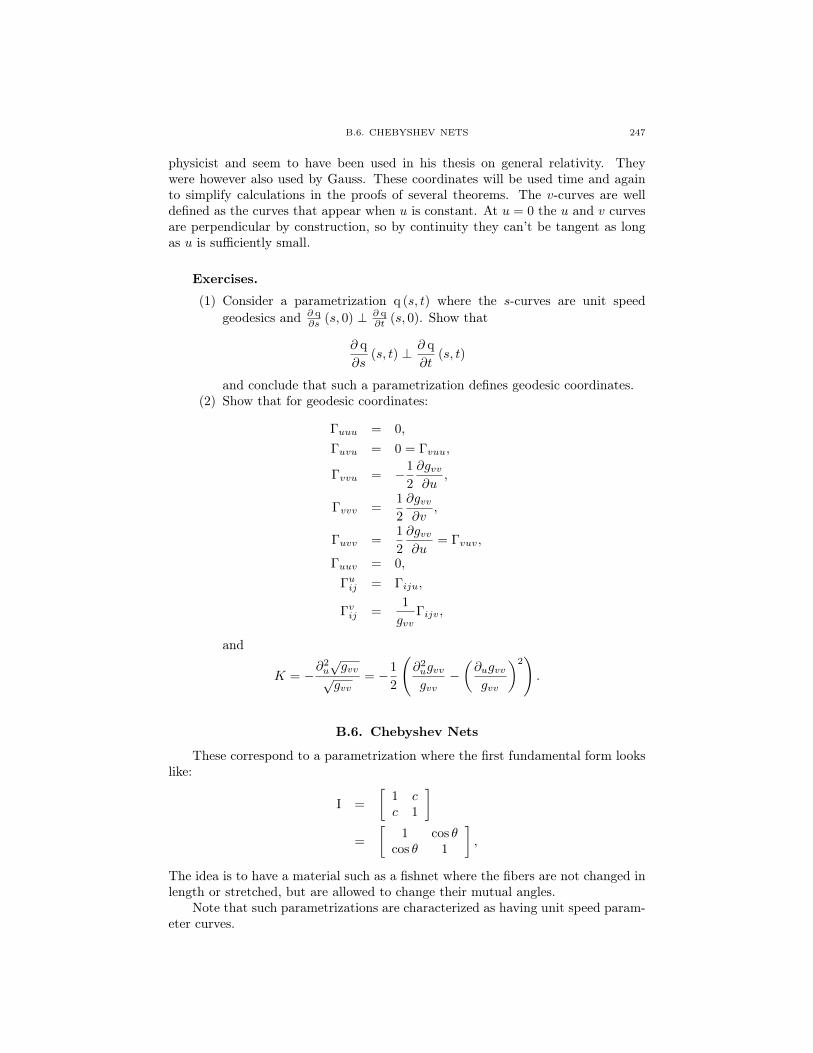
B.6. CHEBYSHEV NETS 247
physicist and seem to have been used in his thesis on general relativity. Theywere however also used by Gauss. These coordinates will be used time and againto simplify calculations in the proofs of several theorems. The v-curves are welldefined as the curves that appear when u is constant. At u = 0 the u and v curvesare perpendicular by construction, so by continuity they can’t be tangent as longas u is sufficiently small.
Exercises.
(1) Consider a parametrization q (s, t) where the s-curves are unit speedgeodesics and ∂ q
∂s (s, 0) ⊥ ∂ q∂t (s, 0). Show that
∂ q
∂s(s, t) ⊥ ∂ q
∂t(s, t)
and conclude that such a parametrization defines geodesic coordinates.(2) Show that for geodesic coordinates:
Γuuu = 0,
Γuvu = 0 = Γvuu,
Γvvu = −1
2
∂gvv∂u
,
Γvvv =1
2
∂gvv∂v
,
Γuvv =1
2
∂gvv∂u
= Γvuv,
Γuuv = 0,
Γuij = Γiju,
Γvij =1
gvvΓijv,
and
K = −∂2u√gvv√gvv
= −1
2
(∂2ugvvgvv
−(∂ugvvgvv
)2).
B.6. Chebyshev Nets
These correspond to a parametrization where the first fundamental form lookslike:
I =
[1 cc 1
]=
[1 cos θ
cos θ 1
],
The idea is to have a material such as a fishnet where the fibers are not changed inlength or stretched, but are allowed to change their mutual angles.
Note that such parametrizations are characterized as having unit speed param-eter curves.

B.7. ISOTHERMAL COORDINATES 248
Exercises.
(1) ???Show that any surface locally admits Chebyshev nets. Hint: Fix apoint p = q (u0, v0) for a given parametrization and define new parameters
s (u, v) =
∫ u
u0
√guu (x, v)dx
t (u, v) =
∫ v
v0
√gvv (u, y)dy
Show that ∂s∂v (u0, v0) = 0 = ∂t
∂u (u0, v0) and conclude that (s, t) defines anew parametrization that creates a Chebyshev net.
(2) Show that Chebyshev nets q (u, v) satisfy the following properties
∂2 q
∂u∂v⊥ TpM,
Γuvw = Γuuu = Γvvv = 0,
Γuuv = −∂θ∂u
sin θ,
Γvvu = −∂θ∂v
sin θ,
∂2θ
∂u∂v= −K sin θ.
(3) Show that the geodesic curvature κg of the u-coordinate curves in a Cheby-shev net satisfy
κg = −∂θ∂u.
(4) (Hazzidakis) Show that√
det [I] = sin θ, and that integrating the Gausscurvature over a coordinate rectangle yields:
−∫
[a,b]×[c,d]
K sin θdudv = 2π − α1 − α2 − α3 − α4
where the angles αi are the interior angles.
B.7. Isothermal Coordinates
These are also more generally known as conformally flat coordinates and havea first fundamental form that looks like:
I =
[λ2 00 λ2
]The proof that these always exist is called the local uniformization theorem. It is nota simple result, but the importance of these types of coordinates in the developmentof both classical and modern surface theory cannot be understated. There is alsoa global result which we will mention at a later point. Gauss was the first to workwith such coordinates, and Riemann also heavily depended on their use. They have

B.7. ISOTHERMAL COORDINATES 249
the properties that
Γuuu =∂ log λ
∂u
Γuvu =∂ log λ
∂v= Γvuu
Γvvv =∂ log λ
∂v
Γuvv =∂ log λ
∂u= Γvuv
Γuuv = −∂ log λ
∂v
Γvvu = −∂ log λ
∂u,
Γw3w1w2
=1
λ2Γw1w2w3 ,
K = − 1
λ2
(∂2 log λ
∂u2+∂2 log λ
∂v2
).
Using complex analysis one obtains isothermal parametrizations as follows. Fora parametrized surface define w = u+ iv and complex functions φi (w), i = 1, 2, 3
φ = (φ1, φ2, φ3) =∂ q
∂w=∂ q
∂u− i
∂ q
∂v.
In other wordsReφ =
∂ q
∂u, Imφ = −∂ q
∂v.
First observe that∂φ
∂w=∂φ
∂u+ i
∂φ
∂v=
∂2 q
∂w∂w=∂2 q
∂u2+∂2 q
∂v2.
So φ is holomorphic if and only if q is harmonic.Next note that
φ21 + φ2
2 + φ23 = φ · φ =
(∂ q
∂u− i
∂ q
∂v
)·(∂ q
∂u− i
∂ q
∂v
)= guu − gvv − 2iguv.
So we obtain an isothermal parametrization when φ21 +φ2
2 +φ23 = 0. The conformal
factor can then be calculated by noting that
φ · φ = |φ1|2 + |φ2|2 + |φ3|2 =
(∂ q
∂u− i
∂ q
∂v
)·(∂ q
∂u+ i
∂ q
∂v
)= guu + gvv.
Conversely, starting with holomorphic functions φi (w), i = 1, 2, 3 such thatφ2
1 + φ22 + φ2
3 = 0 we can define their antiderivatives and construct a surface by
q (w) =
(2Re
(∫φ1 (w) dw
), 2Re
(∫φ2 (w) dw
), 2Re
(∫φ3 (w) dw
))since ∂Ref
∂w = 12
(∂f∂w + ∂f
∂w
)= 1
2∂f∂w , when f (w) is holomorphic and consequently f
antiholomorphic.A minimal surface evidently always has such a parametrization: First use that
the Gauss map is conformal to conclude that it has an isothermal parametrization.This must be harmonic which in turn shows that φ is holomorphic since.
Examples:

B.7. ISOTHERMAL COORDINATES 250
Catenoid: φ1 = sinhw, φ2 = −i coshw, φ3 = 1.Helicoid: φ1 = i sinhw, φ2 = coshw, φ3 = i.Enneper: φ1 = 1− w2, φ2 = i
(1 + w2
), φ3 = 2w.
Scherk: φ1 = 21+w2 , φ2 = 2i
1−w2 , φ3 = 4w1−w4 .
Catalan: φ1 = 1− cosh (−iw), φ2 = i sinh (−iw), φ3 = 2 sinh(− iw
2
).
Can always use φ1 = F(1−G2
), φ2 = iF
(1 +G2
), and φ3 = 2FG with
2F = φ1 − iφ2.
Exercises.(1) A particularly nice special case occurs when
λ2 (u, v) = U2 (u) + V 2 (v)
These types of metrics are called Liouville metrics. Compute their Christof-fel symbols, Gauss curvature, and show that when geodesics are writtenas v (u) or u (v) they they solve a separable differential equation. Showalso that the geodesics have the property that
U2 sin2 θ − V 2 cos2 θ
is constant, where θ is the angle the geodesic forms with the u curves.(2) Show that when
λ =1
a (u2 + v2) + buu+ bvv + c
we obtain a metric with constant Gauss curvature
K = 4ac− b2u − b2vIt can be shown that no other choices for λ will yield constant curvature.

Bibliography
[1] D. Hilbert and S. Cohn-Vossen, Geometry and the Imagination, New York: Chelsea, 1990.[2] H. Hopf, Differential Geometry in the Large. 2nd Ed. LNM 1000, Springer Verlag, 1989[3] D.J. Struik, Lectures on Classical Differential Geometry, New York: Dover, 1988.
251


