CMBFIT : Rapid WMAP likelihood calculations with normal parameters
Havard B. Sandvik,* Max Tegmark, and Xiaomin WangDepartment of Physics, University of Pennsylvania, Philadelphia, Pennsylvania 19104, USA
Matias ZaldarriagaDepartment of Physics, Harvard University, Cambridge, Massachusetts 02138, USA
~Received 3 December 2003; published 18 March 2004!
We present a method for ultrafast confrontation of the Wilkinson Microwave Anisotropy Probe~WMAP!cosmic microwave background observations with theoretical models, implemented as a publicly availablesoftware package calledCMBFIT, useful for anyone wishing to measure cosmological parameters by combiningWMAP with other observations. The method takes advantage of the underlying physics by transforming into aset of parameters where the WMAP likelihood surface is accurately fit by the exponential of a quartic or sexticpolynomial. Building on previous physics based approximations by Huet al., Kosowskyet al., and Chuet al.,it combines their speed with precision cosmology grade accuracy. AFORTRAN code for computing the WMAPlikelihood for a given set of parameters is provided, precalibrated againstCMBFAST, accurate toD ln L;0.05over the entire 2s region of the parameter space for 6 parameter ‘‘vanilla’’LCDM models. We also provide7-parameter fits including spatial curvature, gravitational waves and a running spectral index.
The impressive sensitivity of the long awaited WilkinsoMicrowave Anisotropy Probe~WMAP! data allows for un-precedented constraints on cosmological models@1–6#. Themeasurements have strengthened the case for the cosmcal concordance model@6#, the inflationary cold dark mattemodel with a cosmological constant (LCDM) model, a flatUniverse which is currently accelerating due to mysteriodark energy, where most matter is in the form of collisionlecold dark matter, and where the initial conditions for tfluctuations are adiabatic. Because of well known cosmmicrowave background~CMB! parameter degeneracie@5,7,8#, the true impressiveness of the data is most cleademonstrated by either imposing reasonable priors, coming the data with complimentary data sets, or both. The mrecent precision data-sets are the Sloan Digital Sky Sur~SDSS! galaxy power spectrum@9# and a new Supernovae Icompilation@10#, and combining these with the WMAP constraints has further narrowed error bars@11#, giving us cos-mological parameters at a precision not thought possonly a few years ago.
So how are CMB data-sets used to estimate parameAlthough constraints on cosmological parameters fromCMB can in principle be extracted directly from the mathemselves, this is effectively prohibited by the huge comtational power necessary to perform the required likelihocalculations~although for a novel approach, see@12#!. In-stead, the more efficient parameter estimation method cmonly employed uses the angular power spectrum ofmap as an intermediate step@13–15#.
Likelihoods on the basis of power spectrum constraiare much faster to calculate, the slowest step being the cputation of the angular power spectrum numerically. T
can be done either through integration of the full Boltzmaequation~with CMBFAST @16# or the modificationsCAMB @17#or CMBEASY @18#! or using an approximate shortcut suchDASH @19#. Although steady improvements in both computpower and algorithm performance have made these calctions significantly faster, the CMB power spectrum likehood calculation is still the bottleneck in any parametertimation process by many orders of magnitude.
Another problem with the estimation process is the nedegeneracies between some cosmological parameters. Egated, banana shaped contours on the likelihood surmake search algorithms less efficient. Several authors hadvocated various transformations from cosmologicalrameters to ‘‘physical’’ parameters more directly linkedfeatures in the power spectrum@7,20#. Chuet al. @21# advo-cated a new such set of ‘‘normal’’ parameters whose prability distributions are well fitted by Gaussian distribution
Our key idea explored in this paper is that if the likehood function is roughly a multivariate Gaussian in the traformed parameters, then it should be very accuratelyproximated by the exponential of a convenient higher-orpolynomial. A Gaussian likelihood surfaceL corresponds tothe log-likelihood lnL being quadratic, and a quadratic Talor expansion is of course an accurate approximation offunction near its maximum. Very far from the maximum, thGaussian approximation again becomes accurate, sinceit and the true likelihoodL are vanishingly small. We willsee that in most cases, small cubic and quartic correctionln L help provide a near-perfect fit toL everywhere. TheWMAP team employed such quartic fits to determine reasable step sizes for their Markov chain Monte Carlo seaalgorithm@6#. Here we go further and show how polynomifits can conveniently store essentially all the cosmologiinformation inherent in the WMAP power spectra. This rduces calculation of CMB likelihoods to simply evaluatinthe exponential of annth order polynomial. AlthoughCMB-
FAST still needs to be run in order to obtain a sufficient sa
SANDVIK et al. PHYSICAL REVIEW D 69, 063005 ~2004!
pling of the likelihood surface, this only has to be done onfor each model space and dataset. For the models explorthis paper, it has already been done and the polynomialefficients have been obtained. The polynomial fit can thusused to run Monte Carlo Markov chains~MCMC! includingvarious non-CMB data-sets many orders of magnitude fasdramatically reducing the need for computing power for cmological parameter estimation purposes involving WMAdata. This is an improvement on importance sampling meods which notoriously deplete the chain of points asadded data sets shift or narrow the confidence regionmeans joint likelihood analyses between WMAP and otsurveys which would previously take weeks or monthscomputer time on a good workstation being finished inafternoon.
As mentioned, the last few years have seen the risecosmological concordance model@5,11,22#, the LCDM flatinflationary cosmology which has been confirmed astrengthened by WMAP, SDSS and new supernova obsetions. However as cosmological ideas and trends changechoose to keep an open mind and allow for extensions to6-parameter inflationaryLCDM model by including modelswith spatial curvature, gravitational waves and a running slar spectral index. To allow the user to include CMB polaization information separately, we also perform separate llihood fits excluding and including WMAP polarization dafor the 6-parameter scenario.
II. METHOD
Our approach in this paper consists of three steps:~i! Acquire a sample of the likelihood surface as a fun
tion of cosmological parameters. This is done through a Mkov chain Monte Carlo sampling of parameter space.
~ii ! Transform from cosmological parameter space inormal parameters. This will make the likelihood surfaclose to Gaussian in these parameters, thereby increasingnificantly the accuracy of the polynomial fit.
~iii ! Fit of the log-likelihood surface to annth order poly-nomial. The polynomial degreen is optimized to thelikelihood-surface sampling density using a training set/tset approach.
Below we describe each of the above steps in detail.
A. The cosmological parameters
We follow standard work@5,22# in the field and param-etrize our cosmological model with the 13 parameters
p5~t,Vk ,VL ,w,vd ,vb , f n ,As ,ns ,a,r ,nt ,b!. ~1!
These parameters are the reionization optical depth,t, cur-vature energy densityVk , the dark energy densityVL , thedark energy equation of statew, the physical dark matter anbaryon densitiesvd[Vdh2 and vb[Vbh2, the fraction ofdark matter that is warm~massive neutrinos! f n , the primor-dial amplitudes and tilts of the scalar and tensor fluctuatirespectivelyAs ,ns ,r ,nt and the running of the scalar tilta.HereAs , ns, r , nt anda are defined as in@5# and @11#. b is
06300
ein
o-e
r,-
h-eItrfn
a
da-
wee
a---
-r-
o
ig-
t
s
the galaxy biasb25Pgalaxy(k)/P(k). For a comprehensivecosmological parameter summary, see Table 1 of@11#.
As stated in the Introduction, we base our work arouthe adiabatic LCDM cosmological model,$t,VL ,vd ,vb ,ns ,As%, a 6-parameter subspace of the 13 prameters. This is close to the minimal number of free paraeters needed to explain the data~the one exception beingns ,which is still consistent with unity! and assumes a pure comological constant and negligible spatial curvature, tenfluctuations, running tilt, warm dark matter or hot dark mater As @5,11#, we also consider models with added ‘‘spicesuch as curvature, tensor contributions and running tilt.confine ourselves to a maximum of 7 parameters per moi.e., to models withLCDM1a 7th free parameter.
B. The likelihood
The fundamental quantity that one wants to estimate isprobability distribution function~PDF! of the parametersvectorp, P(pud), given the data,d, and whatever prior assumptions and knowledge we may have about the pareters. The quantity we directly evaluate, however, isprobability of measuring the data given the parameteP(dup) through a goodness-of-fit test. It is this distributiowhen thought of as a function of the parameters, thatrefer to as thelikelihood, L(p)[P(dup). The probabilitydistribution function for the parameters is then related tolikelihood through Bayes’ theorem,
P~pud!}P~dup!Pprior~p! ~2!
wherePprior is the prior probability distribution of the parameters.
For ideal, full-sky, noiseless experiments, exact likelihocalculation is simple and fast. However, due to foregroucontamination~the galaxy, point sources, etc.!, only a frac-tion of the sky can be used for analysis. This leads to colations between different multipoles and it becomes comtationally prohibitive to calculate the exact likelihoofunction. Consequently, various approximations existwhich much work has been focused@6,23# ~for an excellentreview of CMB likelihood calculations see@24#!. In all ourWMAP likelihood calculations we employ the latest versioof the likelihood approximation routines supplied by thWMAP team. These routines take all effects into accouuse an optimal combination of the various approximatioand are well tested through simulations@6#. As input, theytake the CMB power spectrum, which we compute wCMBFAST.
C. Fitting to an nth order polynomial
Let us now look at how the polynomial fit is performeddetail. We start with a sample ofN pointsp1 , . . . ,pN in thed-dimensional parameter space where the likelihoodL(p)has been evaluated, and wish to fit lnL(p) to a polynomial.Let ^p& denote the average of the parameter vectorspi in oursample and letC[^ppt&2^p&^p& t denote the correspondincovariance matrix. To improve the numerical stability of o
5-2
er
y
xne-
t
m
-
ha
w,
ri-
a
too
6De-odgherto
s.
of
uchand
n-trib-in
theets,tlycanta
t
oodthethecals toe 6ial
ide
se al-
at
ts376
CMBFIT: RAPID WMAP LIKELIHOOD CALCULATION S . . . PHYSICAL REVIEW D 69, 063005 ~2004!
fitting, we work with transformed parameters that have zmean and unit covariance matrix:1
z[E~p2^p&!, ~3!
whereE is a matrix satisfyingECEt5I so that^zzt&5EŠ(p2^p&)(p2^p&) t
‹Et5I , the identity matrix. There are mansuch choices ofE—we make the choice where the rows ofEare the eigenvectors of the parameter covariance matriCdivided by the corresponding eigenvalues, so our traformed parametersz can be interpreted as simply uncorrlated eigenparameters rescaled so that they all vary onsame scale~with unit variance!. This transformation turnsout to be crucial, changing the matrix-inversion below froquite ill-conditioned to numerically well-conditioned.
An nth order polynomial in thesed transformed parameters hasM5(n1d
n )5(n1d)!/n!d! terms:
y[ logL5q01(i
q1i zi1 (
i 1< i 2q2
i 1i 2zi 1zi 2
1 (i 1< i 2<•••< i d
qni 1i 2••• i dzi 1
zi 2•••zi d
. ~4!
We assemble all necessary products ofzi ’s into anM-dimensional vector
and the corresponding coefficientsq into anotherM-dimensional vector
q5$q0 ,q11 , . . . ,q1
d ,q111, . . . ,qn
d . . . d , . . . %, ~6!
which simplifies Eq.~4! to
y5x•q. ~7!
We now assemble theN measured log-likelihoodsyi fromour Monte Carlo Markov chain into anN-dimension-al vector y and the correspondingx-vectors into an(N3M )-dimensional matrixX, so theN-dimensional vectorof residual errors« from our polynominal fit is
«[y2Xq. ~8!
We choose the fit that minimizes the rms residual, i.e., tminimizes u«u2. Differentiating with respect toq gives thestandard least-squares result
q5~XtX!21Xty. ~9!
Thus minimizing the sum of squares in the end comes doto the inversion of anM3M matrix. The size of the matrixM5(n1d)!/n!d!, depends on both the number of parameters and the polynomial degree, ranging fromM5210 for a
1The advantage of diagonalizing the parameter covariance mwas also pointed out by@21#.
06300
o
s-
he
t
n
-
6-parameter 4th order fit toM51716 for a 7-parameter 6thorder fit ~see Table I for the number of coefficients for vaous relevant cases!.
Chu et al. @21# have illuminated the problems of fittingGaussian directly to the 6-~or higher! dimensional likelihoodsurfaces and have argued that the surfaces may besparsely sampled in these dimensions. Consequently@21# fitsto the 2D marginalized distributions and reconstructs thelikelihood function from this. Our interpretation is that thdifficulties with fitting a quadratic polynomial to the 6- or 7dimensional log-likelihood surface shows that the likelihosurface deviates too much from a Gaussian and that a hiorder polynomial is required to reproduce the likelihoodsufficient accuracy. This interpretation is shared by@6# whouse a 4th order polynomial to calculate MCMC step size
It is an advantage of our approach that we donot relystrictly on the chain we fit to being a fair statistical samplethe likelihood. Indeed we only need thevalue of the likeli-hood at a sufficient number of points, and we are as sinsensitive to statistical errors such as sampling errorspoor mixing. The way that the input pointspi sample param-eter space tells the fitting algorithm how important we cosider residuals in various places. Since our points are disuted as the WMAP likelihood itself, the fit will be accuratethose parts of parameter space that are consistent withdata. If our fits are combined with complementary data shigh accuracy is of course only necessary in the small joinallowed region of parameter space, and this accuracyoptionally be further improved by including non-CMB dato determine how to sample the CMB likelihood surface.
Clearly the sample size~the number of steps in the inpuMonte Carlo Markov chain! along with the dimensionality ofthe parameter space determines how densely the likelihsurface is sampled. In order to make a best possible fit for7-parameter models we therefore include the points from6-parameter chain in the fit, thus placing extra statistiweight on the vanilla parameter substance. This allows uuse the higher parameter fit to get excellent results for thparameter case as well in addition to reducing polynomartifacts.
Of course the polynomial has complete freedom outsthe sampled region, which means that for degreen.2 the fitwill generally blow up in regions far from the origin. Thimeans that once a search algorithm ventures outside th
rix
TABLE I. Number of coefficients for a model withd parametersfitting to an nth order polynomial. The number of coefficienranges from 28 for a 6-parameter 2nd order fit to a whopping 12for an 11 dimensional model and 6th order polynomial.
SANDVIK et al. PHYSICAL REVIEW D 69, 063005 ~2004!
lowed region, it may find unphysical areas of huge likehoods, much higher than the real maximum. We find thatartifact is efficiently eliminated by replacing the polynomifit by a Gaussiany5e2r 2/2 outside some large radiusr[uzu5(z1
21•••1zd2)1/2 in the transformed parameter spac
To ensure that we do not introduce significant polynomartifacts within the sampled region, we use a standard tring set/test set approach. We run the fit on, e.g., 70% ofchain and test the fit on the remainder of the chain. Aspolynomial degree is increased, the training errors will inetably get smaller since there are more degrees of freedwhile the polynomial eventually develops unphysical smascale wiggles in between sample points. This problemquantified by measuring the errors in the test set, allowingto identify the optimal polynomial degree as the point whethe test set error is minimized. In the limit of very largsample sizeN, the test and training errors approach the savalue for any given polynomial degreen.
D. Markov chain Monte Carlo
To make an accurate polynomial fit, we need a sufficienlarge sample of the likelihood surface as a function ofcosmological parameters. This is done by Markov chMonte Carlo ~MCMC! sampling of the parameter spacthrough the use of the Metropolis-Hastings algorithm@25–34#. When implemented correctly, this is a very effectimethod for explorations of parameter space, and we brireview the concept here. What we want is to genersamplespi , i 50,1,2, . . . from the probability distributionP(p) of Eq. ~2!. The method consists of the following step
~i! We start by choosing a starting pointp0 in parameterspace, and evaluate the corresponding value of the probity distribution P(p0).
~ii ! Next we draw a candidate pointpi 11 from aproposaldensityQ(pi 11upi) and calculate the ratio
a5Q~pi upi 11!
Q~pi 11upi !
P~pi 11!
P~pi !. ~10!
~iii ! If a>1 we accept this new point, add the new pointthe chain, and repeat the process starting from the new pIf a,1, we accept the new state with probabilitya, other-wise we reject it, write the current state to the chainagainand make another draw from the proposal densityQ.
After an initial burn-in period which depends heavily othe initial position in parameter space~the length of thisburn-in can be as short as 100 steps whilst some chainshave not converged after several thousand steps!, the chainstarts sampling randomly from the distributionP(x), allow-ing for calculation of all relevant statistics such as meansvariances of the parameters. The choice of proposal denis of great importance for the algorithm performance asdefines a characteristic step size in parameter space.small a value and the chain will exhibit poor mixing, aexcessive step size and the chain will converge very slosince almost all candidate points get rejected. The acceptratio is a common measure of how successful a chainHowever, whereas a low acceptance ratio certainly dem
06300
is
.ln-ee-m,-iss
e
e
yen
yte
il-
nt.
till
dityitoo
lyces.n-
strates poor performance, high acceptance ratio can bartifact of too small step size, which makes successive poin the chain highly correlated. As discussed in@11#, a betterfigure of merit is the chaincorrelation length, as it deter-mines the effective number of independent points inchain.
Our particular MCMC implementation is described in Apendix A of @11#, and gradually optimizes the proposal desity Q(p8up) using the data itself. Once this learning phasecomplete~typically after about 2000 steps, which are thdiscarded!, our proposal densityQ(p8up) is a multivariateGaussian in the jump vectorp82p with the same covariancematrix as the sample pointspi themselves. This guaranteeoptimum performance of theMETROPOLISalgorithm by mini-mizing the number of jumps outside high confidence regiowhilst still ensuring good mixing. A very similar eigenbasapproach to jumping has been successfully used in othecent MCMC codes, notably@21,26,35#.
For each case described in the next section we geneseveral chains, with different initial conditions, which wpass through a number of convergence and mixing tgiven in @6# and @25#.
E. CMB observables and normal parameters
The issue of what we can actuallymeasurefrom the CMBis of fundamental importance, since it helps to clarify whiconstraints come directly from the CMB and which costraints can only be found by combining CMB with othcosmological probes. This has been studied in detail byet al. @7#, who suggested that much of the then availainformation in the temperature power spectrum could in fbe compressed into only four observables, the overall hzontal position of the first peak plus 3 peak height ratiThis work was revisited by the WMAP team@4# and others@36,37# have similarly studied the effects of the parameteincluding dark energy, on CMB peak locations and spacinFrom such studies one can understand the degeneracietween cosmological parameters, by studying their effectthese quantities.2
Kosowskyet al. @20# go further along these lines and propose a set of ‘‘physical’’ parameters to which the power sptrum C,’s have an approximately linear response. Thislows for fast calculation of power spectra around the fiducmodel. The approach was taken further by@21# in realizingthat a linear response to these parameters in theC,’s shouldresult in the logarithm of the likelihood function being werepresented by a 2nd order polynomial, i.e., the likelihofunction should be close to Gaussian in these parameThis approach resulted in another, similar set of paramedubbed ‘‘normal,’’ since they had an approximately normdistribution.
In this work, we use a best of all worlds approach aemploy a core set of normal parameters which are a com
2This work predates WMAP and other recent CMB surveys. Tenormous improvement in the data will by itself have reduceddegeneracies to some degree, adding more information to the pspectrum.
5-4
rase
het
pee-h
g
en.
atp
islyofi-i
m
doue-
-
ofto
ou
a
a
-
last
last
thebyby
maledpt
firstince
CMBFIT: RAPID WMAP LIKELIHOOD CALCULATION S . . . PHYSICAL REVIEW D 69, 063005 ~2004!
nation of the choices available in the above mentioned liteture, with some improvements. We use a coreof 6 parameters corresponding to the flatLCDM model.Specifically, $t,VL ,Vdh2,Vbh2,ns ,As% cast into$e22t,Qs
E ,h3 ,h2 ,t,Ap%. These new parameters are tphysical damping due to the optical depth, an analytic fitthe angle subtended by the acoustic scale, the 1st-to-3rdratio, the 1st-to-2nd peak ratio with tilt dependence removthe physical effect ofns ~e.g., tilt!, and the fluctuation amplitude at the WMAP pivot point. We will now go througthem in detail one by one.
1. The acoustic scale parameter,Qs
The comoving angular diameter distance at decouplingiven by
DA~adec!5c
H0E
adec
1 dx
AVkx21Vdex
(123w)1Vmx~11!
where we have ignored radiation density since the momof interest, decoupling, is well within matter dominatioNote that the integrand is a function of onlythree param-eters,Vk ,Vde and w. If we assume that the scale factordecoupling is constant, the integral is also dependent uonly these three parameters.
Although a numerical evaluation of the above integraltrivial, it is not as fast as we would wish and would quickbecome the dominant obstacle in the polynomial likelihocalculation. There are several reasonably good analyticting formulas out there@7#. However none of them are accurate enough for our needs, so we also perform a polynomfit for DA . We rewrite the expression for the angular diaeter distance as
DA~a!'DA~a!E5c
H0
2
AVm
3d~Vk ,VL ,w! ~12!
where d is an analytic approximation to the integral anequals 1 for a matter dominated universe. We factorAVm5A12Vk2VL to remove a troublesome inverssquare root which is difficult to fit with a polynomial expansion. We fitd(Vk ,VL ,w) with a 5th order polynomial ex-pansion, done by calculatingd numerically for several hundred thousand points in (Vk ,VL ,w)-space and fitting to thissample. Our main errors then come from the assumptionconstant recombination redshift; however this fit is goodthe ;0.1% level, and performs notably better than the fit@7# for nonflat (VkÞ0) and dynamical dark energy (wÞ21) scenarios. This fit can be downloaded as part ofpublicly availableCMBFIT software package.
The comoving sound horizon at decoupling is defined
r s5E0
tdeccs~ t !dt
a~ t !~13!
wherecs(t) is the sound speed for the baryon-photon fluidtime t, well approximated by
06300
-t
oak
d,
is
nt
on
dt-
al-
t
aof
r
s
t
cs25
1
3~113rb/4rg!21. ~14!
Using the relationdt/a5da/(a2H) and the Friedman equation, we can write this similarly to Eq.~11!
r s~adec!51
H0A3E
0
adec
3
S 113Vb
4VgxD 21/2
dx
@~Vkx21Vdex
123w1Vmx1V r !#1/2
.
~15!
If we assume that vacuum energy can be ignored atscattering, this can be readily integrated to give
r s52A 3
3H0AVm
@R* ~11z* !#21/2ln
3A11R* 1AR* 1r * R*
11Ar * R*
~16!
where the photon-baryon and radiation-matter ratios atscattering are given by@7,38#
R* [3rb~z* !
4rg~z* !530vb~z* /103!21 ~17!
r * [r r~z* !
rm~z* !50.042vm
21~z* /103!, ~18!
with a redshift of last scattering
z* '1048~110.00124vb20.738!~11g1vm
g2! ~19!
g150.0783vb20.238~1139.5vb
0.763!21 ~20!
g250.560~1121.1vb1.81!21. ~21!
The sound horizon and the angular diameter distance attime of decoupling combine to give the angle subtendedthe sound horizon at last scattering. In degrees, it is given
Qs[r s~adec!
DA~adec!
180
p. ~22!
This has been verified to be an excellent choice for a norparameter@20,21# and is indeed one of the best constraincosmological parameters@5,9#. We use this parameter, excereplacing the exact integralsDA(adec) and r s(adec) withtheir analytic approximations, Eqs.~12! and ~16!.
2. The peak ratios h2 , h3 and the scalar tilt parametert
Hu et al. @7# ~and the recent reanalysis of@4#! define pa-rameter fits to the ratios of the 2nd and 3rd peaks to thepeak. Again these are near ideal normal parameters s
5-5
owr
tInerre
-
-
cththcyethf
he
aternisw
weolhe
he
tion
m-
n
sti-hein
byisllehis
at
nde-ict-
ains
is
SANDVIK et al. PHYSICAL REVIEW D 69, 063005 ~2004!
they are directly measurable from the power spectrum. Hever there is one problem. Our requirement is a parametewith which to replace the cosmological parameters.H3 ismostly dependent onVmh2 andH2 most heavily dependenon Vbh2—however, they both also depend on the tilt.other words, three cosmological parameters come togethform two observables. Thus to obtain a corresponding thparameter set, we factor out the tilt dependence fromH2~Pageet al. @4#! and H3 ~Hu et al. @7#! and create the variable set$h2 ,h3 ,t%, where
The parametert is given by a slight modification of the formula used by@21# in order to minimize correlation withvb
t5S vb
0.024D20.5233
2ns21. ~25!
3. The amplitude at the pivot point
For the amplitude we again use the choice of@21#. Thischoice removes the near perfect degeneracy with the opae22t due to a nonzero optical depth. It also evaluatesamplitude at a more optimal pivot point rather than atarbitrary k50.05 Mpc21, such as to remove degenerawith the tilt ns . However we make two modifications: Wchange the choice of pivot-point, as this is dependent ondata set and needs to be updated to optimize resultsWMAP. We also remove a strong correlation withvm em-pirically. The resulting formula is
A* 5Ase22tS k
kpivotD ns21
vm20.568, ~26!
wherekpivot50.041 Mpc21 ~this choice minimizesDA* /A*using WMAP temperature and polarization information; tcorresponding optimal value iskpivot50.037 Mpc21 usingWMAP temperature information alone!.
4. The nonvanilla parameters,vL , a and r
For the 7-parameter case where the assumption of spflatness is relaxed, the choice of an extra normal parametnot obvious. Since we useQs as one of our parameters, iprinciple any of$VL ,Vk ,h% could be used. Since therenow an extra free component in the Friedman equation,choose instead to go with thephysicaldark energy densityvQ[VQh2. This has most of the desirable propertiesseek, and consequently it gives very small errors in the pnomial fit. We could in fact equally well have chosen t
06300
-set
toe-
ityee
eor
ialis
e
y-
physicalcurvature densityvk[Vkh2 as this gives very simi-
lar results. Both perform significantly better than any of tabove three.
The running of the tilt is defined asa5dn/d ln k. Whentaken as a free 7th parameter, it has a distribution funcwhich is very nearly Gaussian~seen in Fig. 6!. Thus we usethis parameter directly as a normal parameter.
For the tensor contribution, we use as our normal paraeter the tensor to scalar ratio,r[At /As , whereAt andAs aredefined earlier as theCMBFAST tensor and scalar fluctuatioamplitudes respectively, evaluated atk50.05 Mpc21.
III. RESULTS
In this section, we present the results of the fits. We emate the errors in the fitting and in particular display tmarginalized likelihoods obtained by running Markov chaMonte Carlo chains using our fits in place ofCMBFAST.
A. Fitting accuracy
In principle a data set may be fitted to any accuracyusing a polynomial of sufficiently high order. However, thwill introduce unphysical polynomial artifacts, which wiruin the method’s applicability. As explained in Sec. II, wtherefore split our data into a training set and a test set. Tallows us to identify the optimal order of the polynomial thwe fit to.
This approach is illustrated for the 6-parameterLCDMcase in Fig. 1, where we plot the fitting accuracy for 2through 7th order polynomials, showing the difference btween test and training sets. The training set errors pred
FIG. 1. rms fitting errorD ln L for the 6-parameterLCDM case.The plot compares the training and test sets for fits based on chusing CMBFAST and chains usingDASH. For the particular chain-length used for theCMBFAST case, we see that a 6th degree fitoptimal.
5-6
nilla
CMBFIT: RAPID WMAP LIKELIHOOD CALCULATION S . . . PHYSICAL REVIEW D 69, 063005 ~2004!
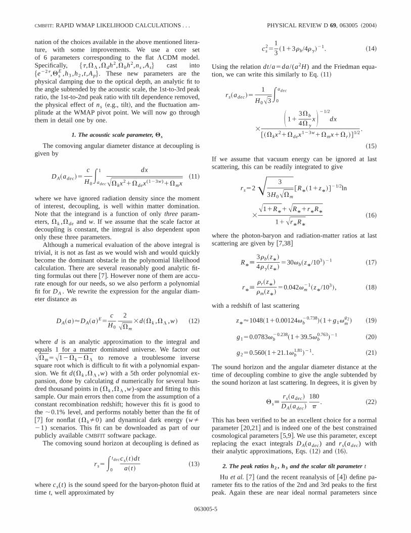
TABLE II. rms polynomial fit errors for all the considered cases, ranging from 6-parameter vaLCDM models to spiced up models including curvature, tensor perturbations, running tilt.
Model Chain origin Chain length Priors Pol. deg.n D ln Ltrain D ln Ltest
6-par T Own 183008 None 6 0.02 0.086-par T1X Own 311391 None 6 0.02 0.056-par1k WMAP 278325 t,0.3 4 0.25 0.366-par1a WMAP 435992 t,0.3 4/5 0.12/0.08 0.14/0.126-par1r Own 178670 None 4 0.29 0.69
re
t.owg4
u-h,
l-h
an
nen
ow
on
sze
e
rix
ahe
ci-o a
ellnsto
oe
ehehe
t isns
der
ionels
-
ably fall with increasing polynomial degree, as there amore degrees of freedom with which to fit the data. The tset errors, however, have a clear minimum~in this case forn56) which is what we choose as optimal polynomial fiThis optimal polynomial degree depends strongly on hlong a chain is used for the fit. A large sample allows us toto higher order, whereas for a small sample, even 3rd ororder polynomials may be ill-fated.
Due to theoretical prejudice for the probability distribtions to be close to Gaussian as well as relatively smootis possible that some of the errors in fitting to theCMBFAST-calculated likelihoods could be due to inaccuracies inCMB-
FAST itself rather than our polynomial approximation. Athough we have not attempted to test or quantify this, tmay be worth exploring in future work.
Figure 1 also shows that we obtained slightly larger rdom scatter when computing power spectra withDASH @19#instead ofCMBFAST. This does not appear to be a limitatioof DASH itself, since the accuracy is greatly improved whusing the latest version ofDASH with transfer functions fromthe latest version ofCMBFAST ~Knox, private communica-tion!. From here on, we useCMBFAST to calculate all ourlikelihood samples.
The mean scatter in the values of lnL range from a good0.05 for the 6th order fit to theLCDM 6-parameter model toa more dubious 0.69 for the 6-parameter1tensor perturbationcase. Accuracies for all the cases are shown in Table II. Hever it is not immediately clear that the error in lnL is nec-essarily the most interesting quantity, as it may include ctributions at low lnL which will have negligible impact onthe relevant parts of the likelihood surface.
An equally interesting quantity isDL5Lf i t2L ~we nor-malizeL to equal unity at its maximum!, which shrinks rap-idly with decreasing values for lnL and thus better illustratewhat kind of accuracies we can expect for the marginalidistributions. The mean scatter in the values ofL is signifi-cantly smaller, typically of order;0.01 for the entiredataset. A better understanding of these quantities canobtained by studying Fig. 2. It shows first how well~or ratherhow badly! the actual likelihood surface~both in terms ofLand lnL) is described by a Gaussian PDF in the transformnormal parameters. These are the variablesz defined in Sec.II C, which have zero mean and identity covariance matand thed-dimensional radius is given byr 5uzu5(z1
21•••
1zd2)1/2. The plot then shows the fitting errorsDL[Lf i t
2L andD ln L5 ln Lf i t2 ln L, plotted as errors relative toGaussian distribution. This visualizes the ability of t
06300
est
oth
it
is
-
-
-
d
be
d
,
method to reproduce the likelihood surface with good presion and the dramatic improvement gained from going tpolynomial degree higher than 2.
B. Application to MCMC
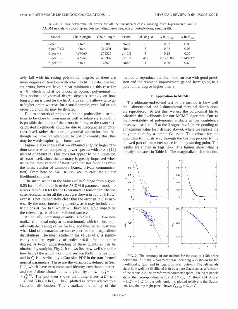
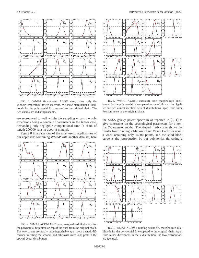
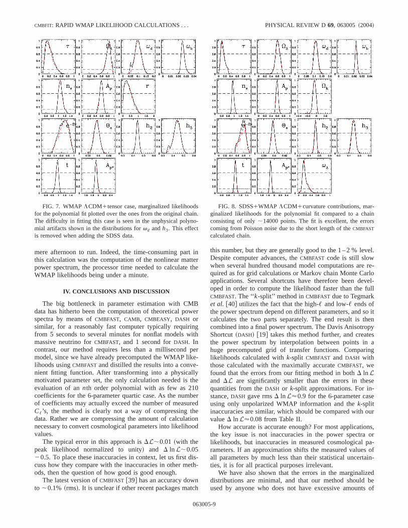
The ultimate end-to-end test of the method is how wthe 1-dimensional and 2-dimensional marginal distributioare reproduced. To test this, we use the polynomial fitscalculate the likelihoods for our MCMC algorithm. Due tthe inevitability of polynomial artifacts at low confidencareas, we use a cutoff at the 3 sigma level~corresponding toa maximum value forr defined above!, where we replace thepolynomial fit by a simple Gaussian. This allows for thalgorithm to find its way through the burn-in process to tallowed part of parameter space from any starting point. Tresults are shown in Figs. 3–7. The figures show whaalready indicated in Table II: The marginalized distributio
FIG. 2. The accuracy of our method for the case of a 5th orpolynomial fit to the 7-parameter case includinga is shown for thelikelihood L ~top! and its logarithm lnL ~bottom!. The left panelsshow how well the likelihood is fit by a pure Gaussian, as a functof the radiusr in the transformed parameter space. The right panshow the corresponding errorsD L[Lf i t2L ~top! and D ln L[ ln Lf i t2 ln L for our polynomial fit, plotted relative to the Gaussian, i.e., the top right panel showsLGauss1Lf i t2L.
5-7
nla
oer
on-
utcka
elihe
rindi
-inme
rt
SANDVIK et al. PHYSICAL REVIEW D 69, 063005 ~2004!
are reproduced to well within the sampling errors, the oexceptions being a couple of parameters in the tensor cdemanding only negligible computational time~a chain oflength 200000 runs in about a minute!.
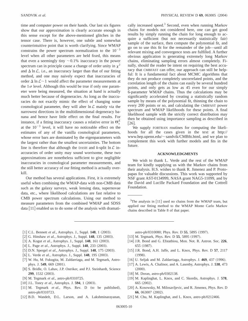
Figure 8 illustrates one of the most useful applicationsour approach: combining WMAP with another data set, h
FIG. 3. WMAP 6-parameterLCDM case, using only theWMAP temperature power spectrum. We show marginalized likhoods for the polynomial fit compared to the original chain. Ttwo chains are indistinguishable.
FIG. 4. WMAPLCDM T1X case, marginalized likelihoods fothe polynomial fit plotted on top of the ones from the original chaThe two chains are nearly indistinguishable apart from a smallference in fitting the second~and otherwise ruled out! peak in theoptical depth distribution.
06300
yse,
fe
the SDSS galaxy power spectrum as reported in@9,11# togive constraints on the cosmological parameters for a nflat 7-parameter model. The dashed~red! curve shows theresults from running a Markov chain Monte Carlo for aboa week obtaining only 14000 points, and the solid blacurve is the reproduction by our polynomial fit, taking
-
.f-
FIG. 5. WMAP LCDM1curvature case, marginalized likelihoods for the polynomial fit compared to the original chain. Agawe see two almost identical sets of distributions, apart from soPoisson noise in the original chain.
FIG. 6. WMAPLCDM1running scalar tilt, marginalized like-lihoods for the polynomial fit compared to the original chain. Apafrom minor differences in thet distribution, the two distributionsare identical.
5-8
ttte
t
Bw
ngit
pke-
yt
0brehtioo
diet
nch
vel.
re-rlovel-ull
so ithenpyes
aing
se
e
our
ns,or
pa-s ofain-
edbe
ts of
-in
rs
sino
CMBFIT: RAPID WMAP LIKELIHOOD CALCULATION S . . . PHYSICAL REVIEW D 69, 063005 ~2004!
mere afternoon to run. Indeed, the time-consuming parthis calculation was the computation of the nonlinear mapower spectrum, the processor time needed to calculateWMAP likelihoods being under a minute.
IV. CONCLUSIONS AND DISCUSSION
The big bottleneck in parameter estimation with CMdata has hitherto been the computation of theoretical pospectra by means ofCMBFAST, CAMB, CMBEASY, DASH orsimilar, for a reasonably fast computer typically requirifrom 5 seconds to several minutes for nonflat models wmassive neutrino forCMBFAST, and 1 second forDASH. Incontrast, our method requires less than a millisecondmodel, since we have already precomputed the WMAP lilihoods usingCMBFAST and distilled the results into a convenient fitting function. After transforming into a physicallmotivated parameter set, the only calculation needed isevaluation of annth order polynomial with as few as 21coefficients for the 6-parameter quartic case. As the numof coefficients may actually exceed the number of measuC,’s, the method is clearly not a way of compressing tdata. Rather we are compressing the amount of calculanecessary to convert cosmological parameters into likelihvalues.
The typical error in this approach isDL;0.01 ~with thepeak likelihood normalized to unity! and D ln L;0.0520.5. To place these inaccuracies in context, let us firstcuss how they compare with the inaccuracies in other mods, then the question of how good is good enough.
The latest version ofCMBFAST @39# has an accuracy dowto ;0.1% ~rms!. It is unclear if other recent packages mat
FIG. 7. WMAP LCDM1tensor case, marginalized likelihoodfor the polynomial fit plotted over the ones from the original chaThe difficulty in fitting this case is seen in the unphysical polynmial artifacts shown in the distributions forvd andh3. This effectis removed when adding the SDSS data.
06300
inrhe
er
h
er-
he
erd
eond
s-h-
this number, but they are generally good to the 1 – 2 % leDespite computer advances, theCMBFAST code is still slowwhen several hundred thousand model computations arequired as for grid calculations or Markov chain Monte Caapplications. Several shortcuts have therefore been deoped in order to compute the likelihood faster than the fCMBFAST. The ‘‘k-split’’ method inCMBFAST due to Tegmarket al. @40# utilizes the fact that the high-, and low-, ends ofthe power spectrum depend on different parameters, andcalculates the two parts separately. The end result is tcombined into a final power spectrum. The Davis AnisotroShortcut~DASH! @19# takes this method further, and creatthe power spectrum by interpolation between points inhuge precomputed grid of transfer functions. Comparlikelihoods calculated withk-split CMBFAST and DASH withthose calculated with the maximally accurateCMBFAST, wefound that the errors from our fitting method in bothD ln Land DL are significantly smaller than the errors in thequantities from theDASH or k-split approximations. For in-stance,DASH gave rmsD ln L'0.9 for the 6-parameter casusing only unpolarized WMAP information and thek-splitinaccuracies are similar, which should be compared withvalueD ln L'0.08 from Table II.
How accurate is accurate enough? For most applicatiothe key issue is not inaccuracies in the power spectralikelihoods, but inaccuracies in measured cosmologicalrameters. If an approximation shifts the measured valueall parameters by much less than their statistical uncertties, it is for all practical purposes irrelevant.
We have also shown that the errors in the marginalizdistributions are minimal, and that our method shouldused by anyone who does not have excessive amoun
FIG. 8. SDSS1WMAP LCDM1curvature contributions, marginalized likelihoods for the polynomial fit compared to a chaconsisting of only;14000 points. The fit is excellent, the errocoming from Poisson noise due to the short length of theCMBFAST
calculated chain.
.-
5-9
rei
thwP
anr
g
a-ac
m
bFo
erwtto
twiba
er
etaov
ttoS
at
voodc-
ndller
ovFi-cu--
atthered
plybe
omto
alyd in
://
e
Pmoto-
bybyrell
tv
SANDVIK et al. PHYSICAL REVIEW D 69, 063005 ~2004!
time and computer power on their hands. Our last six figushow that our approximation is clearly accurate enoughthis sense except for the above-mentioned glitches intensor case. There is, however, one subtle and somecounterintuitive point that is worth clarifying. Since WMAconstrains the power spectrum normalization to the 1023
level when all other parameters are held fixed, this methat even a seemingly tiny;0.1% inaccuracy in the powespectrum can in principle cause a change of order unity inx2
andD ln L, i.e., an inaccuracy larger than that of our fittinmethod, and one may naively expect that inaccuraciesorderD ln L;1 would affect the parameter measurementsthe 1s level. Although this would be true if only one parameter were being measured, the situation at hand is actumuch better because of degeneracies. As long as the inaracies do not exactly mimic the effect of changing socosmological parameter, they will alter lnL mainly via thenarrowest directions in the multidimensional degeneracynana and hence have little effect on the final results.instance, if a fitting inaccuracy causes a relative error inQs
E
at the 1023 level, it will have no noticeable effect on thestimates of any of the vanilla cosmological parametewhose error bars are dominated by the eigenparametersthe largest rather than the smallest uncertainties. The boline is therefore that although theDASH and k-split lnL in-accuracies of order unity may sound worrisome, theseapproximations are nonetheless sufficient to give negliginaccuracies in cosmological parameter measurements,the still better accuracy of our fitting method is actually ovkill.
Our method has several applications. First, it is extremuseful when combining the WMAP-data with non-CMB dasuch as the galaxy surveys, weak lensing data, superndata, etc., where likelihood calculations are fast relativeCMB power spectrum calculations. Using our methodmeasure parameters from the combined WMAP and SDdata@11# enabled us to do some of the analysis with dram
o-
n
n
06300
sne
hat
s
oft
llycu-e
a-r
s,ithm
olend-
ly
aeo
Si-
cally increased speed.3 Second, even when running Markochains for models not considered here, one can get gresults by simply running the chain for long enough to aquire a sufficient ~but not necessarily statistically fair!sample of the surface, then compute the polynomial fit, ago on to use this fit for the remainder of the job—until arelevant mixing and convergence tests are fulfilled. A furthobvious application is generating extremely long Markchains, eliminating sampling errors almost completely.nally, should the reader be intent on requiring the best acracy thatCMBFAST can offer, our approach can still be helpful: It is a fundamental fact about MCMC algorithms ththey do not produce completely uncorrelated points, andcorrelation length of the chains can easily be several hundpoints, and only gets as low as 45 even for our sim6-parameter WMAP chains. Thus the calculations maysignificantly accelerated by creating a statistically randsample by means of the polynomial fit, thinning the chainevery 200 points or so, and calculating theCMBFAST powerspectrum and WMAP likelihoods for these points. A finlikelihood sample with the strictly correct distribution mathen be obtained using importance sampling as describe@26#.
We supply FORTRAN routines for computing the likeli-hoods for all the cases given in the text at httpwww.hep.upenn.edu/;sandvik/CMBfit.html, and we plan tocomplement this work with further models and fits in thfuture.
ACKNOWLEDGMENTS
We wish to thank L. Verde and the rest of the WMAteam for kindly supplying us with the Markov chains frotheir analysis. H.S. wishes to thank R. Jimenez and P. Prpapas for valuable discussions. This work was supportedNSF grant AST-0134999, NASA grant NAG5-11099, andthe David and Lucille Packard Foundation and the CottFoundation.
3The analysis in@11# used no chains from the WMAP team, buapplied our fitting method to the WMAP Monte Carlo Markochains described in Table 8 of that paper.
D
@1# C.L. Bennettet al., Astrophys. J., Suppl.148, 1 ~2003!.@2# G. Hinshawet al., Astrophys. J., Suppl.148, 135 ~2003!.@3# A. Kogut et al., Astrophys. J., Suppl.148, 161 ~2003!.@4# L. Pageet al., Astrophys. J., Suppl.148, 233 ~2003!.@5# D.N. Spergelet al., Astrophys. J., Suppl.148, 175 ~2003!.@6# L. Verdeet al., Astrophys. J., Suppl.148, 195 ~2003!.@7# W. Hu, M. Fukugita, M. Zaldarriaga, and M. Tegmark, Astr
phys. J.549, 669 ~2001!.@8# S. Bridle, O. Lahav, J.P. Ostriker, and P.J. Steinhardt, Scie
299, 1532~2003!.@9# M. Tegmarket al., astro-ph/0310725.
@10# J.L. Tonryet al., Astrophys. J.594, 1 ~2003!.@11# M. Tegmark et al., Phys. Rev. D ~to be published!,
astro-ph/0310723.@12# B.D. Wandelt, D.L. Larson, and A. Lakshminarayana
ce
,
astro-ph/0310080; Phys. Rev. D55, 5895~1997!.@13# M. Tegmark, Phys. Rev. D55, 5895~1997!.@14# J.R. Bond and G. Efstathiou, Mon. Not. R. Astron. Soc.226,
655 ~1987!.@15# J.R. Bond, A.H. Jaffe, and L. Knox, Phys. Rev. D57, 2117
~1998!.@16# U. Seljak and M. Zaldarriaga, Astrophys. J.469, 437 ~1996!.@17# A. Lewis, A. Chalinor, and A. Lasenby, Astrophys. J.538, 473
~2000!.@18# M. Doran, astro-ph/0302138.@19# M. Kaplinghat, L. Knox, and C. Skordis, Astrophys. J.578,
665 ~2002!.@20# A. Kosowsky, M. Milosavljevic, and R. Jimenez, Phys. Rev.
66, 063007~2002!.@21# M. Chu, M. Kaplinghat, and L. Knox, astro-ph/0212466.
5-10
x,
g
tt
.
n-
s.
ev.
CMBFIT: RAPID WMAP LIKELIHOOD CALCULATION S . . . PHYSICAL REVIEW D 69, 063005 ~2004!
@22# X. Wang, M. Tegmark, and M. Zaldarriaga, Phys. Rev. D65,123001~2002!.
@24# A.F. Jaffe, J.R. Bond, P.G. Ferreira, and L.E. Knoastro-ph/0306506.
@25# D.J.C. MacKay,Information Theory, Inference and LearninAlgorithms~Cambridge University Press, Cambridge, 2003!.
@26# A. Lewis and S. Bridle, Phys. Rev. D66, 103511~2002!.@27# L. Knox, N. Christensen, and C. Skordis, Astrophys. J. Le
578, L95 ~2001!.@28# N. Christensen and R. Meyer, astro-ph/0006401.@29# N. Metropolis, A.W. Rosenbluth, M.N. Rosenbluth, A.H
Teller, and E. Teller, J. Chem. Phys.21, 1087~1953!.@30# W.K. Hastings, Biometrika57, 97 ~1970!.@31# W.R. Gilks, S. Richardson, and D.J. Spiegelhalter,Markov
06300
.
Chain Monte Carlo in Practice~Chapman & Hall, London,1996!.
@32# A. Gelman and D. Rubin, Stat. Sci.7, 457 ~1992!.@33# N. Christensen, R. Meyer, L. Knox, and B. Luey, Class. Qua
tum Grav.18, 2677~2001!.@34# A. Slosar and M. Hobson, astro-ph/0307219.@35# O. Zahn and M. Zaldarriaga, Phys. Rev. D67, 063002~2003!.@36# M. Doranet al., Astrophys. J.559, 501 ~2001!.@37# M. Doran and M. Lilley, Mon. Not. R. Astron. Soc.330, 965
~2002!.@38# W. Hu and N. Sugiyama, Phys. Rev. D51, 2599~1995!.@39# U. Seljak, N. Sugiyama, M. White, and M. Zaldarriaga, Phy
Rev. D68, 083507~2003!.@40# M. Tegmark, M. Zaldarriaga, and A.J.S. Hamilton, Phys. R