MATHEMATICAL BIOSCIENCES http://math.asu.edu/˜mbe/AND ENGINEERINGVolume 1, Number 2, September 2004 pp. 243–266

COALGEBRAIC STRUCTURE OF GENETIC INHERITANCE

Jianjun Tian

Department of Mathematics, University of CaliforniaRiverside, CA 92521-0135, USA

Bai-Lian Li

Department of Botany and Plant Sciences, University of CaliforniaRiverside, CA 92521-0124, USA

(Communicated by Yang Kuang)

Abstract. Although in the broadly defined genetic algebra, multiplicationsuggests a forward direction of from parents to progeny, when looking fromthe reverse direction, it also suggests to us a new algebraic structure — coalge-

braic structure, which we call genetic coalgebras. It is not the dual coalgebraicstructure and can be used in the construction of phylogenetic trees. Math-

ematically, to construct phylogenetic trees means we need to solve equationsx[n] = a, or x

(n) = b. It is generally impossible to solve these equations inalgebras. However, we can solve them in coalgebras in the sense of tracing

back for their ancestors. A thorough exploration of coalgebraic structure ingenetics is apparently necessary. Here, we develop a theoretical framework of

the coalgebraic structure of genetics. ¿From biological viewpoint, we definedvarious fundamental concepts and examined their elementary properties thatcontain genetic significance. Mathematically, by genetic coalgebra, we mean

any coalgebra that occurs in genetics. They are generally noncoassociative andwithout counit; and in the case of non-sex-linked inheritance, they are cocom-

mutative. Each coalgebra with genetic realization has a baric property. Wehave also discussed the methods to construct new genetic coalgebras, includ-ing cocommutative duplication, the tensor product, linear combinations and

the skew linear map, which allow us to describe complex genetic traits. Wealso put forward certain theorems that state the relationship between gameticcoalgebra and gametic algebra. By Brower’s theorem in topology, we prove

the existence of equilibrium state for the in-evolution operator.

1. Genetic motivation. While modern genetic inheritance initiated with the the-ory of Charles Darwin, it was the Augustinian Monk Gregor Mendel, who first dis-covered the mathematical character of heredity. In his first paper [1], Mendel ex-ploited some symbolism, which is quite algebraically suggestive, to express his law.In fact, it was later termed “Mendelian algebras” by several authors. In the 1920sand 1930s, general genetic algebras were introduced. Apparently Serebrowsky [2]was the first to give an algebraic interpretation of the sign “×”, which indicatedsexual reproduction, and to give a mathematical formulation of the Mendelianlaws. Glivenkov [3]continued to work at this direction and introduced the so-calledMedelian algebras for diploid populations with one locus or with two unlinked loci.

2000 Mathematics Subject Classification. 16W99.Key words and phrases. general genetic algebras, general genetic coalgebras, baric coalgebras,

conilpotent coalgebras, in-evolution operators.

243

244 J. TIAN, B. LI

Independently, Kostitzin [4] also introduced a “symbolic multiplication” to expressthe Medelian laws. The systematic study of algebras occurring in genetics was dueto I. M. H. Etherington. In his series of seminal papers [5], he succeeded in givinga precise mathematical formulation of Mendel’s laws in terms of non-associativealgebras. He pointed out that the nilpotent property is essential to these geneticalgebras and formulized it in his definition of train algebra and baric algebra. Healso introduced the concept of commutative duplication by which the gametic alge-bra of a randomly mating population is associated with a zygotic algebra. BesidesEtherington, fundamental contributions have been made by Gonshor [6], Schafer [7]Holgate [8, 9], Hench [10], Reiser [11], Abraham [12], Lyubich, and Worz-Busekros[13]. During the early days in this area, it appeared that general genetic algebrasor broadly defined genetic algebra, (by these terms we mean all algebras or anyalgebra having been used in genetics,) can be developed into a field of independentmathematical interest, because these algebras are in general not associative and donot belong to any of the well-known classes of non-associative algebras such as Liealgebra, alternative algebra, or Jordan algebra. They possess some distinguishedproperties that lead to many interesting mathematical results. For example, baricalgebra, which has nontrivial representation over the underlying field, and trainalgebra, whose coefficients of rank equation are only functions of the image underthis representation, are new objectives for mathematicians. From the viewpointof mathematics, Gonshor’s and Schafer’s papers are particularly important. Theyintroduced the (narrowly defined) concept of “genetic algebra” mathematically andproved two fundamental theorems on the existence and uniqueness of idempotentsand on the convergence behavior of sequences of plenary powers in special trainalgebras. Until 1980, the most comprehensive reference in this area was Worz-Busekros. More recent results and direction, such as evolution in genetic algebras,can be found in the book of Lyubich’s work [13]. A good survey article is Reed’s[14].

General genetic algebras are the product of interaction between biology andmathematics. Mendel’s genetics offers a new object to mathematics: generalgenetic algebras. The study of these algebras reveals the algebraic structure ofgenetics, which always simplifys and shortens the way to understand genetic andevolutionary phenomena. Indeed, it is the interplay between the purely mathe-matical structure and the corresponding genetic properties that makes this area sofascinating. However, we found that a very important aspect of Mendelian ge-netics is lost concerning the existing various genetic algebras, because Mendeliangenetic processes in itself implies two directions: forward from parents to progeny,and backward from progeny to their ancestors. Multiplication (referred to sexualreproduction), while it suggests an evolutionary dynamics over generations, wasonly considered, in general genetic algebras, in a direction from parents to theirprogeny. By looking at the genetic processes in the backward direction, we putforward a new algebraic structure—general genetic coalgebras. From mathematicalviewpoint, they are interesting objectives, with new concepts and new elements putforward, such as a character of coalgebra, baric coalgebras, co-powers, co-nilpotent,and so on. It will also become a new foundation and perspective to study geneticinheritance.

This new mathematical framework could help evolutionary biologists to traceback through generations over time and space in search of certain common ances-tors or ancestral distributions. For example, in general genetic algebras, we study

GENETIC COALGEBRAS 245

the sequences of plenary powers or principle powers, x[n] or x(n), to look for thegenetic information after n generations from the initial generation x. However,when we know the present generation y, and want to trace back for the genetic in-formation of n generations before, we need to solve equations x[n] = y or x(n) = y.Generally, it is imposible to solve these equations in algebras. This is the mainreason one gives restriction of low-degree polynomials (rank) when people studygeneral nonassociative algebras. In our proposed coalgebraic structure, we cansolve these equations in the sense of dynamic viewpoint. That is, we once viewcomultiplication as the backward dynamic process whenever we think of multipli-cation as forward dynamic process, then we just need to take plenary co-powersor principle co-powers, ∆[n] (y) = x or ∆(n) (y) = x. This way, we provide amethod for evolutionary biologists to trace back through generations over time andspace in search of certain common ancestors, and to construct the phylogenetictrees. Since any genetic algebra is not sufficient to study evolutionary processes,a thorough exploration of coalgebraic structure in genetics is necessary.

The article is organized as follows: In section 2, we recall the basic concepts inboadly defined genetic algebras, particularly algebras with genetic realization andtheir dual coalgebras. In this section we will note that these dual coalgebras cannot give us the genetic information when we study backward evolution, constructphylogenetic trees. In section 3, we introduce the coalgebras with genetic realiza-tion, which is the basic genetic coalgebras. As examples of this, we will study thegametic coalgebras, the zygotic coalgebras and the co-commutative duplications.In section 4, we will discuss elementary properties of the general genetic coalge-bras, in particular, the baric coalgebras and their genetic aspect. In section 5, wewill discuss methods to construct new genetic coalgebras from simple ones whichcorresponds to complex genetic traits. In section 6, we will introduce various co-powers and co-nilpotent coalgebras that are essentially important in constructingphylogenetic trees. In section 7, we introduce the in-evolution operators and dis-cuss their properties that can be used to specify the tracing path. Finally, we postsome interesting open questions in section 8.

2. The basic genetic algebras and their dual coalgebras. In this section, werecall some basic definitions in general genetic algebras and give their dual coal-gebraic structure, which may offer a different perspective about genetic algebras.These dual coalgebras themselves do not provide any new information about theunderlying genetic processes, but they serve as a starting point for us to develop anew coalgebraic structure that will provide new genetic information.

2.1. The Basic Genetic Algebras. By a population space, we mean that a vector

space, Ω, spanned by a set ei, | i ∈ Λ, which are free over the real number field R,where the generator set ei, | i ∈ Λ is a certain genotype set or a hereditary typeset that is related to a trait that we are interested in, and Λ is an index set whichis usually finite, although it may be infinite. Now, we can define a linear map mfrom the tensor product space Ω ⊗ Ω to Ω as follows:

m : Ω ⊗ Ω −→ Ω

m (ei ⊗ ej) =

n∑

k=1

γkij ek, i, j = 1, 2, · · · , n

246 J. TIAN, B. LI

and linearly extend m (ei ⊗ ej) onto Ω ⊗ Ω. These structural coefficients satisfy0 ≤ γk

ij ≤ 1 and∑n

k=1 γkij = 1. Then, the vector space Ω becomes an algebra.

We call the pair (Ω,m), in a general sense, a basic genetic algebra. Generally,a basic genetic algebra is not associative. Its biological significance is that whenthree genotypic parents cross to beget genotypic grandsons, there are two differentcombinations of crossing. As a result, the genotype of grandsons arising from twodifferent combinations of crossing are generally different. Some authors call analgebra defined by this way an algebra with genetic realization. Lyubich call itstochastic algebra when it is commutative. Two examples follow: the gameticalgebras and zygotic algebras.

2.1.1. The gametic algebras. We consider an infinitely large randomly mating pop-ulation of diploid individuals which differ genetically at several autosomal loci andcan be represented by genetically finitely distinct gametes as our population spaceΘ. We denote these geneticall distinct gametes by ei, i = 1, 2, · · ·, n, then Θ isspanned by these gametes:

Θ =

n∑

i=1

αiei | αi ∈ R, i = 1, 2, · · ·, n .

If we take the standard n-dimensional complex in the linear space Rn and denoteit by S0, there is a bijection between the state set of the population space and S0.For convenience, we denote a subspace of Θ by Θ0, which is linearly isomorphic toS0. Then, each vector, x =

∑ni=1 αiei, in Θ0 represents a state of the population,

and the coefficient αi of ei is the frequency of the gamete ei. For the multiplicationm (ei ⊗ ej) =

∑nk=1 γk

ijek, i, j = 1, 2, · · ·, n, the structural coefficient γkij can be

interpreted as the probability that the zygote ei ⊗ ej produces the gamete ek. Itis clear that, when we consider non-sex-linked inheritance, the gametic algebra iscommutative and not associative. Specifically, the structural coefficients satisfy anadditional condition

γkij = γk

ji, i, j, k = 1, 2, · · ·, n.

2.1.2. The zygotic algebras. In a way similar to constructing a gametic algebra, wecan construct a zygotic algebra. Let eij be a kind of zygote that is begotten fromtwo kinds of genetically different gametes. Then, we can represent the zygote as

eij = ei ⊗ ej , i ≤ j, i, j = 1, 2, · · ·, n,

where ei and ej are gametes. We also denote the zygote space by Z

Z =

n∑

i,j=1,i≤j

αijeij | αij ∈ R, i ≤ j, i, j = 1, 2, · · ·, n

.

Random mating of zygotes eij and epq in the population yields zygote eks withprobability γij,pq,ks. And the multiplication is given by

m (eij ⊗ epq) =∑

k≤s

γij,pq,kseks, i ≤ j, p ≤ q, i, j, p, q = 1, 2, · · ·, n.

These coefficients satisfy:

0 ≤ γij,pq,ks ≤ 1,

n∑

k,s=1,k≤s

γij,pq,ks = 1, and γij,pq,ks = γpq,ij,ks,

GENETIC COALGEBRAS 247

where i ≤ j, p ≤ q, i, j, p, q = 1, 2, · · ·, n.Thus, we get the basic zygotic algebras.

2.2. The dual coalgebras of basic genetic algebras. Now, we define the co-population space to be the linear dual space of the population space,

Ω∗ = f | f : Ω −→ R, is a linear map .

The dual basis ηi | i ∈ Λ is called a co-genotype or co-hereditary type set, whichsatisfies ηi (ej) = δij , where δij is Kronecker delta. There is a dual coalgebraicstructure over Ω∗. Its comultiplication is given by the composition

∆ : Ω∗ m∗

−→ (Ω ⊗ Ω)∗

ρ−1

−−→Ω∗ ⊗ Ω∗,

where map ρ is the bijection from the tensor space Ω∗⊗Ω∗ to (Ω ⊗ Ω)∗, since Ω is fi-

nite dimensional. Explicitly, the composition says 〈∆(f) , a ⊗ b〉 = 〈f,m (a ⊗ b)〉 =〈f, ab〉 , for each f ∈ Ω∗ and a ⊗ b ∈ Ω ⊗ Ω.

If we write the comultiplication as ∆ (ηk) =∑

i,j αijk ηi ⊗ ηj , then

〈∆(ηk) , ei ⊗ ej〉 = 〈ηk, ei · ej〉 =

⟨

e∗k,

n∑

l=1

γlijel

⟩

=

n∑

l=1

γlij 〈e

∗k, el〉 = γl

ij

so we have

∆ (ηk) =

n∑

i,j=1

γkijηi ⊗ ηj .

Thus, we get the dual coalgebra (Ω∗,∆). When the coefficients satisfy 0 ≤γk

ij ≤ 1, and∑n

k=1 γkij = 1, it is the dual basic genetic coalgebra, and, in general it

is not coassociative.

Remark 1. We give an interpretation of the definition as follows. If we take thegametic space Θ as the population space Ω here, we will get the co-gametic spaceΘ∗, and we call ηk to be a co-gamete, and ηi ⊗ ηj to be a co-zygote. Thecoefficient γk

ij is still the probability that a co-zygote ηi ⊗ ηj produces a co-gameteηk. Thus, we will get the dual coalgebra of the gametic algebra (Θ∗,∆). Similarly,we can get the dual coalgebra of the zygotic algebra. Although the summation in thecomultiplication operation is taken in a different way, this coalgebra is “equivalent”to the original algebra to describe various gametes’ or zygotes’ genetic situations.This also means that we will not obtain new information about genetic processesfrom dual coalgebras, which just gives us a different viewpoint. Pursuing differentcoalgebras or coalgebraic structures in order to study genetic evolutionary problemsis needed, which is the focus of this paper.

3. The basic genetic coalgebras. In this section, we will define the basic geneticcoalgebras. We will use the term “general genetic coalgebra(s)” or “broadly definedgenetic algebras” for any coalgebra or all coalgebras used in genetics, and to avoidany confusion, we will not use the term “genetic coalgebra.” As examples, we willgive the gametic coalgebras, and the zygotic coalgebras. We will also put forwardan approach—cocommutative duplication, which can be used to construct a newgenetic structure from the old ones to reveal some more genetic information. For

248 J. TIAN, B. LI

example, we can construct zygotic coalgebraic structures from gametic coalgebraicstructures. We will also give the relation between gametic algebras and gameticcoalgebras under certain specific conditions.

3.1. The gametic coalgebras. Let Θ be the gametic space, e1,e2, · · ·, en be thegenetically distinct gametes in this space, every element, ai ⊗ aj , in tensor productspace Θ⊗Θ, can be viewed as a zygote. Now, we trace from a gamete back to its“parental generation” to see various possibilities that those parents can “beget” thisgamete. Then, if a gamete ek comes from a zygote of type ei ⊗ ej with probabilityβk

ij , we define a comultiplication as follows:

∆ : Θ −→ Θ ⊗ Θ

∆(ek) =n∑

i,j=1

βkij ei ⊗ ej , k = 1, 2, · · ·, n

and linearly extend it onto Θ. The coefficients satisfy

0 ≤ βkij ≤ 1 and

n∑

i,j=1

βkij = 1, i, j, k = 1, 2, · · ·, n.

Then we call pair (Θ,∆) gametic coalgebra.

Remark 2. In general, this gametic coalgebra is not coassociative. That is, thecoassociativity (id ⊗ ∆) ∆ = (∆ ⊗ id) ∆ is not satisfied. When we trace froma gamete back to “its grandparental generation” along distinct individuals in “itsparental generation,” we will get different distributions of probabilities of the geno-type of two generations ago that gave rise to the gamete.

Remark 3. In the study of the inheritance of non-sex-linked traits, this coalgebra iscocommutative; that is, τ∆ = ∆, where τ is the permutation of Θ⊗ Θ, τ (a ⊗ b) =b ⊗ a. Or, structural coefficients satisfy βk

ij = βkji , i, j, k = 1, 2, · · ·, n. In some

special cases, it is not cocommutative.

Remark 4. In general, there is no counit; that is, there is no coalgebraic map εfrom Θ to R , such that (id ⊗ ε) ∆ = id = (ε ⊗ id) ∆. However, we will giveanother concept, character, to describe a similar property later.

As an example, let’s consider a randomly mating population of diploid individu-als that differ in a locus alleles e1,e2, · ··, en; then, the population space is spannedby e1, e2, · · ·, en . We can still use them to indicate the genetically distinct ga-metes. Since comultiplication is determined by structural coefficients, we give thesecoefficients as follows:

βkij =

1

2n(δik + δjk) , i, j, k = 1, 2, · · ·, n.

Let’s look at a special case: when e1 = A, e2 = a, we have

∆ (A) =1

2A ⊗ A +

1

4A ⊗ a +

1

4a ⊗ A,

and

∆ (a) =1

4A ⊗ a +

1

4a ⊗ A +

1

2a ⊗ a.

GENETIC COALGEBRAS 249

3.2. The zygotic coalgebras. For simplicity, we denote the zygote ei ⊗ej by eij ,Then, our population space will be the zygotic space spanned by

eij , i ≤ j, i, j = 1, 2, · · ·, n

where we consider each eij to be genetically distinct zygotes in a population. Wealso think eij and eji are the same type of zygote here. The zygotic space Z isthe same as that in Section 2. For each zygote eij , we trace back to its parentalgeneration to see the probability distribution of zygotes in its parental generationinvolved. Or, we consider the zygote eij comes from two zygotes epq and est in

its parental generation with probability βijpq,st. Then, we have:

0 ≤ βijpq,st ≤ 1, βij

pq,st = βijst,pq

i ≤ j, p ≤ q, i, j, p, q, s, t = 1, 2, · · ·, n,

and∑

p≤q,s≤t

βijpq,st = 1, i, j = 1, 2, · · ·, n.

We define the comultiplication for basis elements:

∆ (eij) =∑

p≤q,s≤t

βijpq,stepq ⊗ est

and linearly extend it onto Z. Thus there is a cocommutative coalgebraic structurein Z, which is not coassociative and without counit. We call the pair (Z,∆) thezygotic coalgebra.

3.3. The cocommutative duplication. First, let us look at an example to seehow to construct a zygotic coalgebra from a gametic coalgebra. Here, we stillconsider non-sex linked traits. Both the gametic coalgebra and the zygotic coal-gebra are cocommutative. We assume that zygotes are formed by random matingof gametes; and gametes are e1, e2, · · ·, en, and zygotes are eij = ei ⊗ ej i ≤ ji, j = 1, 2, · · ·, n. It is clear that the probability of zygote eij coming from zygotesepq and est is the product of the probabilities that the gamete ei comes from zy-gote epq and the probabilities that the gamete ej comes from zygote est. Sinceeij = eji, we should add these probabilities appropriately. Then the comultiplica-

tion coefficients, βijpq,st, of zygotic coalgebra Z are obtained by the comultiplication

coefficient βipq of gametic coalgebra Θ as follows:

βijpq,st =

βipqβ

jst + βi

stβjpq i ≤ j

βipqβ

ist i = j

Thus, we have derived the zygotic coalgebra from the gametic coalgebra. We callthis process cocommutative duplication of the gametic coalgebra. We give thedefinition as follows:

Definition 3.1. Let (C,∆) be a cocommutative coalgebra, Σ be a subspace of thetensor product C ⊗ C, which is given by

Σ =

∑

i∈I

(xi ⊗ yi − yi ⊗ xi) | xi, yi ∈ C, i ∈ I, |I| < ∞

.

The equivalent class of x ⊗ y in the quotient, the symmetric tensor product,C ⊗ C/Σ = C ∨ C is denoted by x ∨ y. We can define comultiplication over this

250 J. TIAN, B. LI

quotient to be

(x ∨ y) =∑

(x),(y)

x(1) ∨ y(1) ⊗ x(2) ∨ y(2)

where ∆(x) =∑

(x) x(1) ⊗ x(2) and ∆(y) =∑

(y) y(1) ⊗ y(2) are Sweedler nota-tions.

Then, the symmetric tensor product with comultiplication forms a cocommu-tative coalgebra. We call (C ∨ C,) the cocommutative duplication of (C,∆) .

3.4. Coalgebras with genetic realization. Let (C,∆) be a coalgebra over afield K. K may be taken as real number field R, if C admits a basis e1, e2 · · ·, en

such that the comultiplication constants βkij with respect to this basis satisfy

0 ≤ βkij ≤ 1 i, j, k = 1, 2, · · ·, n

andn∑

i,j=1

βkij = 1, k = 1, 2, · · ·, n

where

∆ (ek) =n∑

i,j=1

βkijei ⊗ ej , k = 1, 2, · · ·, n.

We say (C,∆) is a coalgebra with genetic realization and its basis is called anatural basis.

Remark 5. Gametic coalgebras and zygotic coalgebra all have a genetic realization.If a coalgebra has a genetic realization, then element e1, e2, · · ·, en of the naturalbasis can be interpreted as genotypes or hereditary types of a population and the realnon-negative number βk

ij can be considered as the probability that ek comes fromei and ej by mating, i, j, k = 1, 2, · · ·, n. If a coalgebra has a natural basis, it mayhave many (finite or even infinite many) natural bases.

Theorem 3.1. Suppose that the population space is a randomly mating diploidpopulation without selection, and non-sex linked and all zygotes have the same fer-tility. If the genetic distinct gametes e1, e2, · · ·, en span the gametic space Θ, thenthe gametic algebra (Θ,m) and the gametic coalgebra (Θ,∆) have the relation

βkij =

γkij

∑ni,j=1 γk

ij

, i, j, k = 1, 2, · · ·, n

where these coefficients are structural constants, that m (ei ⊗ ej) =∑n

k=1 γkijek,

i, j = 1, 2, · · · , n and ∆(ek) =∑n

i,j=1 βkijei ⊗ ej , k = 1, 2, · · · , n.

Proof. Since it is non-sex linked, the gametic algebra (Θ,m) is commutative andthe gametic coalgebra (Θ,∆) is cocommutative. By the definition of the gameticalgebra, γk

ij is the probability that zygote ei ⊗ ej produces gamete ek, and since

there is no selection, we can think of γkij as the number that zygote ei⊗ej produces

gametes ek. Then the total number of gamete ek would be∑n

i,j=1 γkij , but γk

ij

gametes ek come from zygote ei ⊗ ej , by the definition of the gametic coalgebra,

βkij =

γkij

∑

ni,j=1

γkij

. We complete the proof.

GENETIC COALGEBRAS 251

4. The baric coalgebras. To characterize various genetic situations by coalge-bras, we need some new specific concepts. In this section, we will put forward thebaric coalgebra which contains certain genetic information.

4.1. The character of a coalgebra.

Definition 4.1. Let (C,∆) be a coalgebra over a field K. A character is definedto be a nonzero coalgebraic map from C to the underlying field K.

That is, if φ is a character, φ is a linear map which preserves the coalgebraicstructure. We take field K as a coalgebra while the comultiplication is taken as∆k (1) = 1 ⊗ 1. Since K ⊗ K ≃ K, character φ satisfies (φ ⊗ φ)∆ = ∆kφ = φ.In fact, the character can be viewed as a representation of C with dimension one.

Remark 6. Since a coalgebra need not to have counit in genetic case, no coalgebraadmits a nonzero character. For instance, coalgebra A with comultiplication∆(x) = 0 has no character. For any character φ, the kernal of φ, kerφ, is acoideal with codimension one as a vector subspace of C, and C⊗C is not containedin ∆(kerφ); that is, C ⊗ C is not contained inkerφ ⊗ C + C⊗kerφ.

Proposition 4.1. Suppose that C is a coalgebra over a field K and C has a char-acter φ, then kerφ is a (n − 1)−dimensional coideal of C and the factor coalgebraC/kerφ is isomorphic to the field K.

Proof. Since (φ ⊗ φ)∆ = φ, so (φ ⊗ φ)∆ (kerφ) = φ (kerφ) = 0, then

∆ (kerφ) ⊆ ker (φ ⊗ φ) = C ⊗ kerφ + kerφ ⊗ C

so kerφ is a coideal. By coalgebraic fundamental isomorphism theorem, the factorC/kerφ has a unique coalgebra structure such that the induced map is a coalgebraisomorphism φ∗ : C/kerφ −→ K. It is clear that the dimension of the kerφ is(n − 1) . We complete the proof.

Theorem 4.1. Let C be a coalgebra over K with characters, then the correspon-dence from character φ to its kerφ is a bijection between the set of characters of Cand the set of coideals Π of codimension one such that C ⊗ C is not contained inΠ ⊗ C + C ⊗ Π.

Proof. First, we prove the onto-ness:Let Π be a coideal with codimensional one, then we have C = C0 ⊕ Π as a

decomposition of vector space, where dim(C0) = 1. We define a map φ : C −→ Kwhich satisfys φ (Π) = 0 and φ (C0) 6= 0 as follows. Take any element e0 ∈ C0

as its basis, for any x ∈ C0, there is x = kxe0, for some kx ∈ K. Then, letφ (x) = kxφ (e0) . Now, linearly extend φ onto C. Thus, it is clear that φ is uniqueup to a scalar coefficient. Let us explain φ is a character for C.

Since C ⊗ C is not contained in Π ⊗ C + C ⊗ Π, we surely have ∆ (e0) =βe0 ⊗ e0 for some nonzero constants β ∈ K. If we set (φ ⊗ φ) ∆ (e0) = φ (e0),then, βφ (e0)φ (e0) = φ (e0). We have φ (e0) = 1

β. Since this β is determined by

comultiplication ∆, so φ is determined uniquely.Now,

∀y ∈ Π, φ (y) = 0

since

∆ (y) ∈ ∆(Π) ⊆ Π ⊗ C + C ⊗ Π, (φ ⊗ φ) ∆ (y) = 0,

252 J. TIAN, B. LI

so,

(φ ⊗ φ) ∆ (y) = φ (y) .

And ∀x ∈ C0, we have

(φ ⊗ φ) ∆ (x) = (φ ⊗ φ) ∆ (kxe0)

= kx (φ ⊗ φ) ∆ (e0) = kxφ (e0)

= φ (kxe0) = φ (x) .

Thus, for any z ∈ C = C0 ⊕ Π, write z = z0 + z1, z0 ∈ C0, and z1 ∈ Π, then

(φ ⊗ φ)∆ (z) = (φ ⊗ φ) (∆ (z0) + ∆ (z1))

= (φ ⊗ φ) ∆ (z0) + (φ ⊗ φ) ∆ (z1)

= φ (z0) = φ(z).

So, φ : C −→ K is a nonzero coalgebraic map. It is a character.Now, we prove the into-ness:If characters φ1 6= φ2, we need show that kerφ1 6=kerφ2. But, if kerφ1 =kerφ2,

according to what have been done above, C = C10⊕ kerφ1 = C2

0⊕ kerφ2, and weget that C1

0 and C20 are the same. Then,

φ1 (e0) =1

β= φ2 (e0) , β =

∆(e0)

e0 ⊗ e0,

Thus, φ1 = φ2. We complete the proof.

4.2. The baric coalgebras.

Definition 4.2. Let (C,∆) be a coalgebra over a field K, if C has a nontrivialcharacter φ, we say that C is a baric coalgebra. Sometimes, we call the characterφ a weight function. We use the notation (C,∆, φ) to denote a baric coalgebra.

Definition 4.3. Let (C,∆, φ) be a baric coalgebra over a field K and C1 be a subsetof C, then C1 is called a baric subcoalgebra if C1 is a subcoalgebra of C and C1 isnot contained in kerφ, or, equivalently, φ1 =: φ |C1

is not zero.

Definition 4.4. Let (C,∆, φ) be a baric coalgebra over a field K and Π be a subsetof C, then Π is called a baric coideal if Π is a coideal of C and Π ⊆ kerφ. In anatural way, the quotient coalgebra C/Π will be a baric quotient coalgebra.

Theorem 4.2. If (C,∆) is a coalgebra over R, which has a genetic realizationwith respect to a natural basis e1, e2, · · ·, en, then (C,∆) is a baric coalgebra.

Proof. We define a character φ : C −→ K by φ (ek) = 1 and linearly extend itonto C. Therefore,

(φ ⊗ φ)∆ (ek) = (φ ⊗ φ)

n∑

i,j=1

βkijei ⊗ ej

=

n∑

i,j=1

βkijφ (ei) ⊗ φ (ej)

=n∑

i,j=1

βkij = 1 = φ(ek)

GENETIC COALGEBRAS 253

and for every x ∈ C, x =∑n

k=1 αkek, we have

(φ ⊗ φ) ∆ (x) = (φ ⊗ φ)

(

n∑

k=1

αk∆(ek)

)

=

n∑

k=1

αk (φ ⊗ φ) ∆ (ek)

=

n∑

k=1

αk = φ (x)

so φ is indeed a character. We finish the proof.

Theorem 4.3. Let (C,∆) be a n-dimensional coalgebra over R; the followingconditions are equivalent:

〈1〉 (C,∆) is baric.〈2〉 (C,∆) has a basis e1, e2, · · ·, en, such that the comultiplication constant can

be defined by

∆ (ek) =

n∑

i,j=1

βkijei ⊗ ej

and satisfiesn∑

i,j=1

βkij = 1, k = 1, 2, · · ·, n.

〈3〉 (C,∆) has a (n − 1)−dimensional coideal Π and C ⊗ C is not contained in∆ (Π).

Proof. 〈1〉 =⇒ 〈2〉 Let φ : C −→ K be a character, then kerφ = Π is a(n − 1)−dimensional coideal of C. Let d2, d3, · · ·, dn be a basis of Π. Since φ isnontrivial, there is an element a ∈ C such that φ (a) 6= 0. Then, set e1 = 1

φ(a)a,

e2 = e1 − d2, e3 = e1 − d3, · · ·, en = e1 − dn. e1, e2, e3, · · · , en forms a basis forC, and φ (ek) = 1, k = 1, 2, · · ·, n. Denote ∆ (ek) =

∑ni,j=1 βk

ijei ⊗ ej . Since

(φ ⊗ φ)∆ (ek) = φ (ek) , we have

(φ ⊗ φ)∆ (ek) = (φ ⊗ φ)

n∑

i,j=1

βkijei ⊗ ej

=

n∑

i,j=1

βkij (φ ⊗ φ) (ei ⊗ ej) =

n∑

i,j=1

βkij

= φ(ek) = 1

Thus, we get∑n

i,j=1 βkij = 1, k = 1, 2, · · ·, n.

〈2〉 ⇒ 〈3〉We define dk = e1 − ek, k = 2, 3, · · ·, n. C0 = 〈d2, d3, · · ·, dn〉 is a subspace

spaned by those elements. We will check that C0 is a (n − 1)−dimensional coideal

254 J. TIAN, B. LI

of C as follows:

∆ (dk) = ∆ (e1 − ek) =

n∑

i,j=1

(

β1ij − βk

ij

)

(ei ⊗ ej)

= −n∑

i,j=1

(

β1ij − βk

ij

)

[(e1 − ei) ⊗ ej − e1 ⊗ ej ]

=

n∑

i,j=1

(

βkij − β1

ij

)

[(e1 − ei) ⊗ ej + e1 ⊗ (e1 − ej) − e1 ⊗ e1]

=

n∑

i,j=1

(

βkij − β1

ij

)

(di ⊗ ej) +

n∑

i,j=1

(

βkij − β1

ij

)

e1 ⊗ dj

∈ C0 ⊗ C + C ⊗ C0

and

∆ (e1) = −

n∑

ij

β1ijdi ⊗ ej −

n∑

ij

e1 ⊗ dj + e1 ⊗ e1

/∈ C0 ⊗ C + C ⊗ C0.

It is done.〈3〉 ⇒ 〈1〉We define φ : C −→ C/Π by x 7−→ x + Π and linearly extend it onto C.

The vector space C/Π is isomorphic to the underlying field K. Since Π is a coidealof C, the map φ is coalgebraic, so C/Π is either isomorphic to K or to zero. Thelatter possibility can be excluded by the dimension one of C/Π. So φ is a characterfunction. Thus, we complete the proof.

Theorem 4.4. Let (C,∆) be a n−dimensional coalgebra over R, then the followingconditions are equivalent:

〈1〉 C has a genetic realization;〈2〉 C is baric and the linear manifold of all elements of weight (the value of the

character function) 1 contain a (n − 1)-dimensional simplex L with ∆ (L) ⊆ L⊗L.

Proof. 〈1〉 =⇒ 〈2〉 Let e1, e2, · · · · ··, en be a natural basis of C. We define a mapφ : C −→ R by φ (ek) = 1 and linearly extend it. Then it is easy to see φ is acoalgebraic map. So C is baric. Let L be the convex hull of e1, e2, · · · · ··, en, then∆ (ek) =

∑nij βk

ijei ⊗ ej ∈ L ⊗ L, so ∆ (L) ⊆ L ⊗ L.

〈2〉 =⇒ 〈1〉 Let φ : C −→ R be any character function. By assumption, thissimplex L is the convex hull of n linearly independent elements e1, e2, ······, en withφ (ek) = 1, k = 1, 2, · · ·, n. These elements form a basis of C. Since ∆ (L) ⊆ L⊗L,if we write ∆ (ek) =

∑ni,j=1 βk

ijei ⊗ ej , these coefficients satisfy 0 ≤ βkij ≤ 1,

i, j, k = 1, 2, · · ·, n. Moreover, since

(φ ⊗ φ) ∆ (ek) = φ (ek) = 1,

GENETIC COALGEBRAS 255

(φ ⊗ φ) ∆ (ek) = (φ ⊗ φ)

n∑

i,j=1

βkijei ⊗ ej

=

n∑

i,j=1

βkijφ (ei)φ (ej) = φ (ek) ,

it is∑n

i,j=1 βkij = 1. We complete the proof.

5. Construction of new genetic coalgebras. To understand the complicatedgenetic situation in term of coalgebras, we need some approaches to construct anew coalgebra from old ones. For example, there are several coalgebras with eachone describing a particular trait in a biological population, so we can combine thesecoalgebras to make a new one in order to describe and model the population. Wewill deal with polyploid individual populations as an example. In this section, wewill discuss the linear combinations of coalgebras, the tensor product of coalgebrasand skew coalgebra by linear maps. In the algebra case, these constructions arewell known. Here we just give some ofthe counterparts in coalgebra motivated byapplications in genetics and skip their detailed proofs.

5.1. Linear combinations. Let V be an n-dimensional vector space over a fieldK, if C is a coalgebra over V , which need not be cocommutative or coassociative,we denote the comultiplication by ∆ (x) = ∆C (x).

Proposition 5.1. Let Co (V ) be the family of all coalgebras over V , for C1, C2 ∈Co (V ); and α ∈ K, the sum C1 + C2, and the scalar product αC1 are defined ascoalgebras over V with comultiplications given by

∆C1+C2(x) = ∆C1

(x) + ∆C2(x)

∆αC1(x) = α∆C1

(x) .

Then, we have(1) Co (V ) is a vector space over K, which is called the vector space of all

coalgebras over V . The zero element of this vector space is the zero coalgebra 0over V .

(2) The family Coc (V ) of all cocommutative coalgeras over V forms a subspaceof Co (V ).

Proof. The proof is skiped here.

Remark 7. (1) This proposition is obvious; we do not need to give a proof here.

(2) It is clear that a linear combination of the coalgebras C1, C2, ··· Cl is∑l

i=1 αiCi,its comultiplication is given by

∆∑

li=1

αiCi(x) =

l∑

i=1

αi∆Ci(x).

(3) If the combination coefficients above are non-negative and sum to one, we callit a convex combination of coalgebras.(4) Coalgebras C1, C2, · · ·, Cr ∈ Co (V ) are called linearly independent if and onlyif the trivial linear combination of these coalgebras is the zero coalgebra.

256 J. TIAN, B. LI

Proposition 5.2. Let e1, e2, ···, en be a basis of V . Then the coalgebras C1, C2, ···, Cr are linearly independent if and only if ∆∑

ri=1

αiCi(ek) =

∑ri=1 αi∆Ci

(ek) =0, k = 1, 2, · · ·, n, which implies that α1 = α2 = · · · = αr = 0.

Proof. We skip it here..

Theorem 5.1. Let C1, C2, · · ·, Cr be baric coalgebras with the same characterfunction φ, then every linear combination

∑ri=1 αiCi with

∑ri=1 αi = 1 is a

baric coalgebra with the character φ.

Proof. For every x ∈ V ,

(φ ⊗ φ) ∆∑

ri=1

αiCi(x) = (φ ⊗ φ)

(

r∑

i=1

αi∆Ci(x)

)

=

r∑

i=1

αi (φ ⊗ φ) ∆Ci(x)

=

r∑

i=1

αiφ (x) = φ (x)

Note K ⊗ K ⊗ · · · ⊗ K ∼= K. So, φ is a character for the coalgebra linearcombination

∑ri=1 αiCi. We prove it.

Theorem 5.2. Let V be a vector space over a field K and C1, C2, · · ·, Cr becoalgebras over V , which have a genetic realization with respect to the same basise1, e2, · · ·, en of V . Then every convex combination of these coalgebras has agenetic realization with respect to e1, e2, · · ·, en.

Proof. We denote the comultiplication constants of coalgebra Ci by βi,kpq , that is to

say

∆Ci(ek) =

n∑

p,q=1

βi,kpq ep ⊗ eq,

thenn∑

p,q=1

βi,kpq = 1 for i = 1, 2, · · ·, r, k = 1, 2, · · ·, n,

and

0 ≤ βi,kpq ≤ 1, for i = 1, 2, · · ·, r, k, p, q = 1, 2, · · ·, n.

Now, for every convex combination∑r

i=1 αiCi, where∑r

i=1 αi = 1 and each αi isnon-negative number, if we write ∆∑

ri=1

αiCi(ek) =

∑np,q=1 λk

pqep ⊗ eq, we need

check that∑n

p,q=1 λkpq = 1 for each k and 0 ≤ λk

pq ≤ 1 for every k, p, q. Let uscompute

∆∑

ri=1

αiCi(ek) =

r∑

i=1

αi∆Ci(ek)

=

r∑

i=1

αi

n∑

p,q=1

βi,kpq ep ⊗ eq

=

n∑

p,q=1

(

r∑

i=1

αiβi,kpq

)

ep ⊗ eq

GENETIC COALGEBRAS 257

so

λkpq =

r∑

i=1

αiβi,kpq .

By Cauchy-Schwarz inequality,

0 ≤ λkpq =

r∑

i=1

αiβi,kpq .

≤

(

r∑

i=1

α2i

)1

2

(

r∑

i=1

(

βi,kpq

)2

)1

2

≤ 1,

andn∑

p,q=1

λkpq =

n∑

p,q=1

r∑

i=1

αiβi,kpq

=r∑

i=1

n∑

p,q=1

αiβi,kpq = 1

We complete the proof.

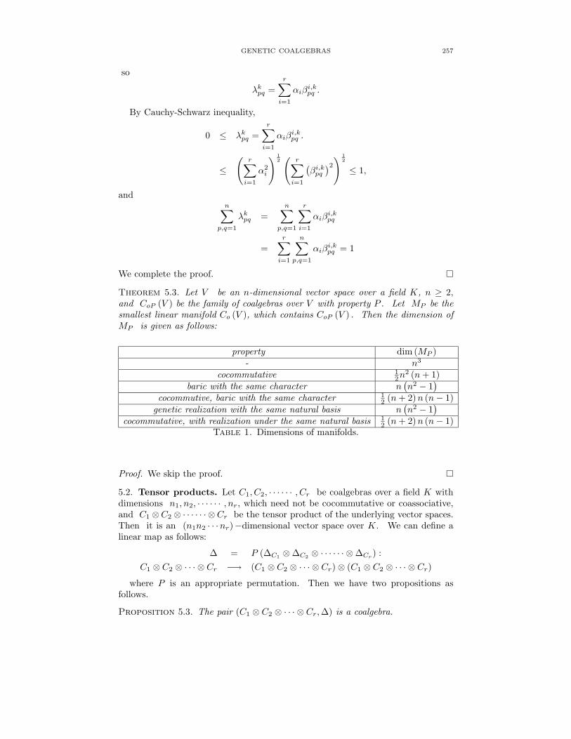
Theorem 5.3. Let V be an n-dimensional vector space over a field K, n ≥ 2,and CoP (V ) be the family of coalgebras over V with property P . Let MP be thesmallest linear manifold Co (V ), which contains CoP (V ) . Then the dimension ofMP is given as follows:

property dim (MP )- n3

cocommutative 12n2 (n + 1)

baric with the same character n(

n2 − 1)

cocommutive, baric with the same character 12 (n + 2)n (n − 1)

genetic realization with the same natural basis n(

n2 − 1)

cocommutative, with realization under the same natural basis 12 (n + 2)n (n − 1)

Table 1. Dimensions of manifolds.

Proof. We skip the proof.

5.2. Tensor products. Let C1, C2, · · · · · · , Cr be coalgebras over a field K withdimensions n1, n2, · · · · · · , nr, which need not be cocommutative or coassociative,and C1 ⊗C2 ⊗ · · · · · · ⊗Cr be the tensor product of the underlying vector spaces.Then it is an (n1n2 · · ·nr)−dimensional vector space over K. We can define alinear map as follows:

∆ = P (∆C1⊗ ∆C2

⊗ · · · · · · ⊗ ∆Cr) :

C1 ⊗ C2 ⊗ · · · ⊗ Cr −→ (C1 ⊗ C2 ⊗ · · · ⊗ Cr) ⊗ (C1 ⊗ C2 ⊗ · · · ⊗ Cr)

where P is an appropriate permutation. Then we have two propositions asfollows.

Proposition 5.3. The pair (C1 ⊗ C2 ⊗ · · · ⊗ Cr,∆) is a coalgebra.

258 J. TIAN, B. LI

Proposition 5.4. If the comultiplication table of factor Ck is given by

∆Ck(ekjk

) =

nk∑

pk,qk=1

βkjkpkqk

ekpk⊗ ekqk

where ek1, ek2, · · · · · · eknk is a basis for Ck, k = 1, 2, · · · r. Then the comulti-

plication table of C1 ⊗ C2 ⊗ · · · ⊗ Cr is given by

n1,n2··· ,nr∑

p1,q1,··· ,pr,qr

β1jip1q1

β2j2p2q2

· · ·βrjrprqr

(e1p1⊗ e2p2

⊗ · · · ⊗ erpr) ⊗ (e1q1

⊗ e2q2⊗ · · · ⊗ erqr

) ,

which is equal to ∆(e1j1 ⊗ e2j2 ⊗ · · · ⊗ erjr)

Proof. We skip the proof.

Now we give two statements that have evident significance for genetics. Becausecomplex traits are affected by multiple factors, we can “tensor” these multiplegenetic factors up as one coalgebra; such a tensor product of coalgebras will appearvery useful to describe polygenetic traits.

Theorem 5.4. Let Ck be a baric coalgebra with character φk, k = 1, 2, · · · · · · r, thenthe tensor product C1⊗C2⊗· · ·⊗Cr is baric with character φ = φ1⊗φ2⊗· · ·⊗φr.

Proof. For any x = x1 ⊗ x2 ⊗ · · · ⊗ xr ∈ C1 ⊗ C2 ⊗ · · · ⊗ Cr, let us verify

(φ ⊗ φ) ∆ (x) = φ (x) .

By (φk ⊗ φk) ∆Ck

(

xk)

= φk

(

xk)

(that is,∑

(xk) φk

(

xk(1)

)

φk

(

xk(2)

)

= φk

(

xk)

),

we have

[(φ1 ⊗ φ2 ⊗ · · · ⊗ φr) ⊗ (φ1 ⊗ φ2 ⊗ · · · ⊗ φr)] ·

[P (∆C1⊗ ∆C2

⊗ · · · · · · ⊗ ∆Cr)](

x1 ⊗ x2 ⊗ · · · ⊗ xr)

=r∑

k=1

∑

(xk)

φk

(

xk(1)

)

φk

(

xk(2)

)

=r∑

k=1

φk

(

xk)

.

We get the proof.

Theorem 5.5. Suppose that each coalgebra Ck has a genetic realization with re-spect to the natural basis ek1, ek2, · · · · · · eknk

, k = 1, 2, · · · , r, then the tensorproduct C1 ⊗ C2 ⊗ · · · ⊗ Cr also has a genetic realization with respect to the basise1j1 ⊗ e2j2 ⊗ · · · ⊗ erjr

| 1 ≤ j1 ≤ n1, 1 ≤ j2 ≤ n2, · · · , 1 ≤ jr ≤ nr .

Proof. Note ∆Ck(ekjk

) =∑nk

pk,qk=1 βkjkpkqk

ekpk⊗ ekqk

and the comultiplication tablein above proposition, it is easy to see

0 ≤ β1jip1q1

β2j2p2q2

· · ·βrjrprqr

≤ 1,

andn1,n2··· ,nr∑

p1,q1,··· ,pr,qr

β1jip1q1

β2j2p2q2

· · ·βrjrprqr

= 1,

since∑nk

pk,qk=1 βkjkpkqk

ekpk= 1, for each k and jk. Thus, we complete the proof.

GENETIC COALGEBRAS 259

5.3. Construction of new genetic coalgebras by linear maps. When weconsider genetic situation of sex-linked inheritance and mutation in a population ofautopolyploid individuals in term of coalgebras, it seems reasonable to introduce askew or new comultiplication by applying a linear map to one factor of the givencomultiplication. We will give some genetic applications later on.

Definition 5.1. Let V be an n-dimensional vector space over a field K, L0, L1,L2 be linear maps from V to V, and C be a coalgebra over V with comultiplication∆. We define a map ∆ to be a composite

∆ = (L1 ⊗ L2) ∆L0 : C −→ C ⊗ C.

Then, the pair(

C,∆)

is a coalgebra over V .

Theorem 5.6. Let V be a vector space over K and C a baric coalgebra over V withcharacter φ. If the linear maps L0, L1,and L2 : V −→ V preserve character;that is, φLi = φ, i = 1, 2, 3, then the coalgebra

(

C,∆)

is baric with character φ.

Proof. By definitions,

(φ ⊗ φ)∆ = (φ ⊗ φ) (L1 ⊗ L2) ∆L0

= (φL1 ⊗ φL2) ∆L0 = (φ ⊗ φ) ∆L0

= φL0 = φ.

we get the proof.

Theorem 5.7. Let (C,∆) be a coalgebra over a vector space V and C have agenetic realization with respect to a natural basis e1, e2, · · ·, en. If the linear mapL0, L1,L2 : V −→ V leaves the simplex

M =

n∑

i=1

αiei | 0 ≤ αi ≤ 1, i = 1, 2, · · · , n,

n∑

i=1

αi = 1

invariant; then the coalgebra(

C,∆)

also has a genetic realization.

260 J. TIAN, B. LI

Proof. Write Lt (ek) =∑n

i=1 αt,ki ei, t = 1, 2, 3, k = 1, 2, · · · , n, then

∑ni=1 αt,k

i =1, since Lt leaves M invariant. We see

∆ (ek)

= (L1 ⊗ L2) ∆L0 (ek)

= (L1 ⊗ L2) ∆

(

n∑

i=1

α0,ki ei

)

=

n∑

i=1

α0,ki (L1 ⊗ L2) ∆ (ei)

=n∑

i=1

α0,k (L1 ⊗ L2)

(

n∑

p,q=1

βipqep ⊗ eq

)

=

n∑

i=1

α0,ki

n∑

p,q=1

βipqL1 (ep)L2 (eq)

=

n∑

i=1

α0,ki

n∑

p,q=1

βipq

n∑

j=1

α1,pj

n∑

s=1

α2,qs ej ⊗ es

=n∑

j,s=1

n∑

i,p,q=1

α0,ki βi

pqα1,pj α2,q

s

ej ⊗ es

By Cauchy-Schwarz inequality, we have

0 ≤

n∑

i,p,q=1

α0,ki βi

pqα1,pj α2,q

s ≤ 1

and

n∑

j,s=1

n∑

i,p,q=1

α0,ki βi

pqα1,pj α2,q

s

= 1

Thus, we complete the proof.

6. Conilpotent coalgebras. In this section, we will define several concepts thatcapture certain interesting genetic features. Since we are considering non-coassociativecoalgebras (which may be or may be not be cocommutative) without counit, weneed to give a kind of order to take comultiplication. The order may give us away to specify the path that traces back over the past generations (phylogeneticgenealogical trees). We first define various copowers, then define conilpotent coal-gebras, which is an analogy of nilpotentness in coalgebraic structure and theirpossible genetic implications. We also give simple propositions and applications asexamples.

GENETIC COALGEBRAS 261

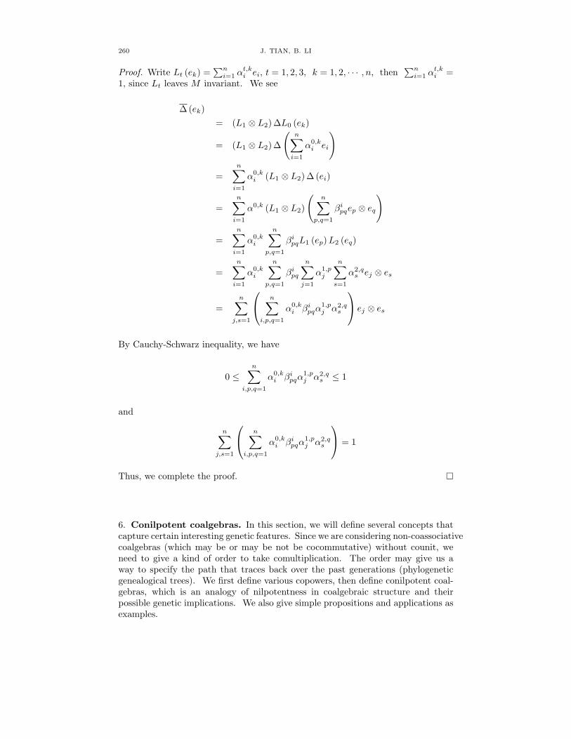
Definition 6.1. Let ∆ be the comultiplication of a coalgebra (C,∆) . We definea copower to be a special order that the comultiplication can be performed consecu-tively. The left principal copower of an element or a subcoalgebra is defined as

1

∆ = ∆2

∆ = (∆ ⊗ id) ∆3

∆ = (∆ ⊗ id ⊗ id) (∆ ⊗ id) ∆

· · · · · · · · · · · · · · · · · · · · ·m

∆ =(

∆ ⊗ id⊗(m−1))m−1

∆ .

Figure 1. Fourth left principle copower of x.

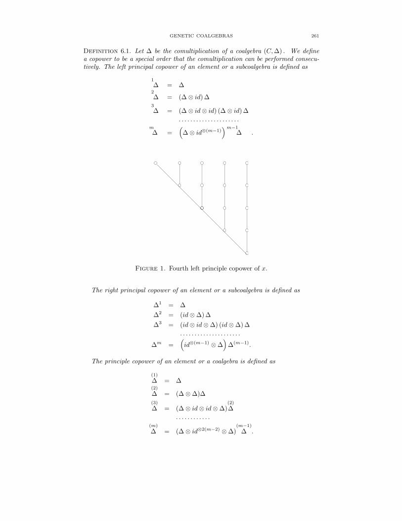
The right principal copower of an element or a subcoalgebra is defined as

∆1 = ∆

∆2 = (id ⊗ ∆) ∆

∆3 = (id ⊗ id ⊗ ∆) (id ⊗ ∆) ∆

· · · · · · · · · · · · · · · · · · · · ·

∆m =(

id⊗(m−1) ⊗ ∆)

∆(m−1).

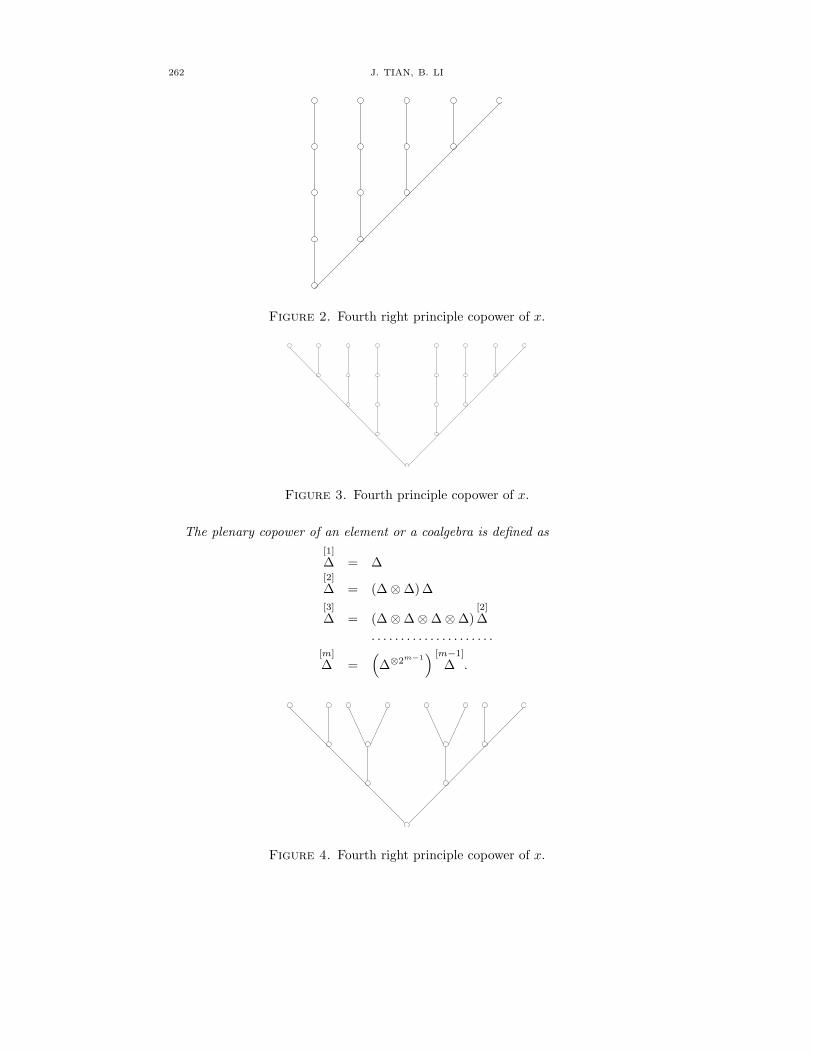
The principle copower of an element or a coalgebra is defined as

(1)

∆ = ∆(2)

∆ = (∆ ⊗ ∆)∆

(3)

∆ = (∆ ⊗ id ⊗ id ⊗ ∆)(2)

∆

· · · · · · · · · · · ·(m)

∆ = (∆ ⊗ id⊗2(m−2) ⊗ ∆)(m−1)

∆ .

262 J. TIAN, B. LI

Figure 2. Fourth right principle copower of x.

Figure 3. Fourth principle copower of x.

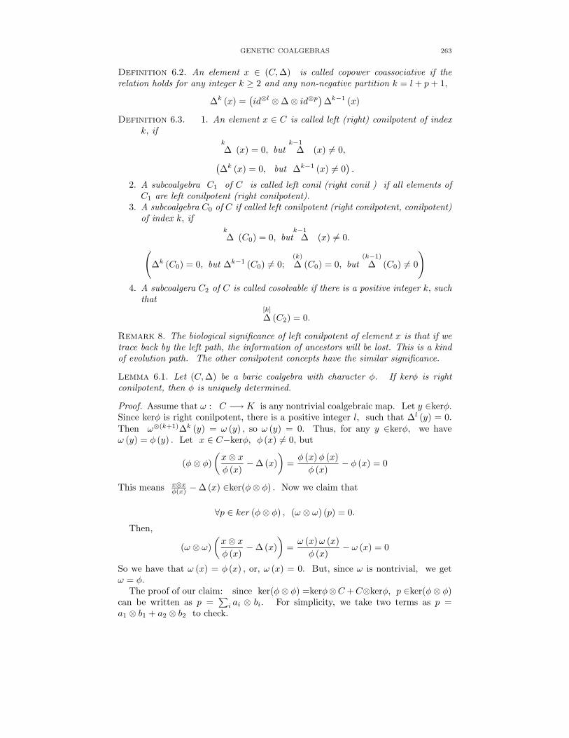
The plenary copower of an element or a coalgebra is defined as

[1]

∆ = ∆[2]

∆ = (∆ ⊗ ∆) ∆

[3]

∆ = (∆ ⊗ ∆ ⊗ ∆ ⊗ ∆)[2]

∆

· · · · · · · · · · · · · · · · · · · · ·[m]

∆ =(

∆⊗2m−1) [m−1]

∆ .

Figure 4. Fourth right principle copower of x.

GENETIC COALGEBRAS 263

Definition 6.2. An element x ∈ (C,∆) is called copower coassociative if therelation holds for any integer k ≥ 2 and any non-negative partition k = l + p + 1,

∆k (x) =(

id⊗l ⊗ ∆ ⊗ id⊗p)

∆k−1 (x)

Definition 6.3. 1. An element x ∈ C is called left (right) conilpotent of indexk, if

k

∆ (x) = 0, butk−1

∆ (x) 6= 0,(

∆k (x) = 0, but ∆k−1 (x) 6= 0)

.

2. A subcoalgebra C1 of C is called left conil (right conil ) if all elements ofC1 are left conilpotent (right conilpotent).

3. A subcoalgebra C0 of C if called left conilpotent (right conilpotent, conilpotent)of index k, if

k

∆ (C0) = 0, butk−1

∆ (x) 6= 0.(

∆k (C0) = 0, but ∆k−1 (C0) 6= 0;(k)

∆ (C0) = 0, but(k−1)

∆ (C0) 6= 0

)

4. A subcoalgera C2 of C is called cosolvable if there is a positive integer k, suchthat

[k]

∆ (C2) = 0.

Remark 8. The biological significance of left conilpotent of element x is that if wetrace back by the left path, the information of ancestors will be lost. This is a kindof evolution path. The other conilpotent concepts have the similar significance.

Lemma 6.1. Let (C,∆) be a baric coalgebra with character φ. If kerφ is rightconilpotent, then φ is uniquely determined.

Proof. Assume that ω : C −→ K is any nontrivial coalgebraic map. Let y ∈kerφ.Since kerφ is right conilpotent, there is a positive integer l, such that ∆l (y) = 0.Then ω⊗(k+1)∆k (y) = ω (y) , so ω (y) = 0. Thus, for any y ∈kerφ, we haveω (y) = φ (y) . Let x ∈ C−kerφ, φ (x) 6= 0, but

(φ ⊗ φ)

(

x ⊗ x

φ (x)− ∆(x)

)

=φ (x)φ (x)

φ (x)− φ (x) = 0

This means x⊗xφ(x) − ∆(x) ∈ker(φ ⊗ φ) . Now we claim that

∀p ∈ ker (φ ⊗ φ) , (ω ⊗ ω) (p) = 0.

Then,

(ω ⊗ ω)

(

x ⊗ x

φ (x)− ∆(x)

)

=ω (x)ω (x)

φ (x)− ω (x) = 0

So we have that ω (x) = φ (x) , or, ω (x) = 0. But, since ω is nontrivial, we getω = φ.

The proof of our claim: since ker(φ ⊗ φ) =kerφ⊗C + C⊗kerφ, p ∈ker(φ ⊗ φ)can be written as p =

∑

i ai ⊗ bi. For simplicity, we take two terms as p =a1 ⊗ b1 + a2 ⊗ b2 to check.

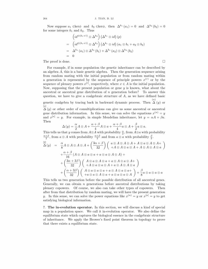
264 J. TIAN, B. LI

Now suppose a1 ∈kerφ and b2 ∈kerφ, then ∆k1 (a1) = 0 and ∆k2 (b2) = 0for some integers k1 and k2. Thus

(

id⊗(k1+1) ⊗ ∆k2

)

(

∆k1 ⊗ id)

(p)

=(

id⊗(k1+1) ⊗ ∆k2

)

(

∆k1 ⊗ id)

(a1 ⊗ b1 + a2 ⊗ b2)

= ∆k1 (a1) ⊗ ∆k2 (b1) + ∆k1 (a2) ⊗ ∆k2 (b2)

= 0

The proof is done.

For example, if in some population the genetic inheritance can be described byan algebra A, this is a basic genetic algebra. Then the generation sequence arisingfrom random mating with the initial population or from random mating withina generation is represented by the sequence of principle powers x(r) or by thesequence of plenary powers x[r], respectively, where x ∈ A is the initial population.Now, supposing that the present population or gene y is known, what about theancestral or ancestral gene distribution of n generation before? To answer thisquestion, we have to give a coalgebraic structure of A, as we have defined basic

genetic coalgebra by tracing back in backward dynamic process. Then(n)

∆ (y) or[n]

∆ (y) or other order of comultiplications can give us some ancestral or ancestralgene distribution information. In this sense, we can solve the equations x(n) = yand x[n] = y. For example, in simple Mendelian inheritance, let y = αA + βa.Then

∆ (y) =α

2A ⊗ A +

α + β

4A ⊗ a +

α + β

4a ⊗ A +

β

2a ⊗ a.

This tells us that y comes from A⊗A with probability α2 , from A⊗a with probability

α+β2 , from a ⊗ A with probability α+β

2 and from a ⊗ a with probability β2 .

[2]

∆ (y) =α

8A ⊗ A ⊗ A ⊗ A +

(

3α + β

32

)(

a ⊗ A ⊗ A ⊗ A + A ⊗ a ⊗ A ⊗ A++A ⊗ A ⊗ a ⊗ A + A ⊗ A ⊗ A ⊗ a

)

+α + β

16(A ⊗ A ⊗ a ⊗ a + a ⊗ a ⊗ A ⊗ A) +

+

(

3α + 3β

32

)(

A ⊗ a ⊗ A ⊗ a + a ⊗ A ⊗ a ⊗ A++A ⊗ a ⊗ a ⊗ A + a ⊗ A ⊗ A ⊗ a

)

+

(

α + 3β

32

)(

A ⊗ a ⊗ a ⊗ a + a ⊗ A ⊗ a ⊗ a++a ⊗ a ⊗ A ⊗ a + a ⊗ a ⊗ a ⊗ A

)

+β

8a ⊗ a ⊗ a ⊗ a

This tells us two generation before the possible distribution of all ancestral genes.Generally, we can obtain n generations before ancestral distributions by takingplenary copowers. Of course, we also can take other types of copowers. Thenafter from that distribution by random mating, we will have the present generationy. In this sense, we can solve the power equations like x(n) = y or x[n] = y to getsatisfying biological information.

7. The in-evolution operator. In this section, we will discuss a kind of specialmap in a population space. We call it in-evolution operator. We also define theequilibrium state which captures the biological essence in the coalgebraic structureof inheritance. We apply the Brower’s fixed point theorem in topology to provethat there exists a equilibrium state.

GENETIC COALGEBRAS 265

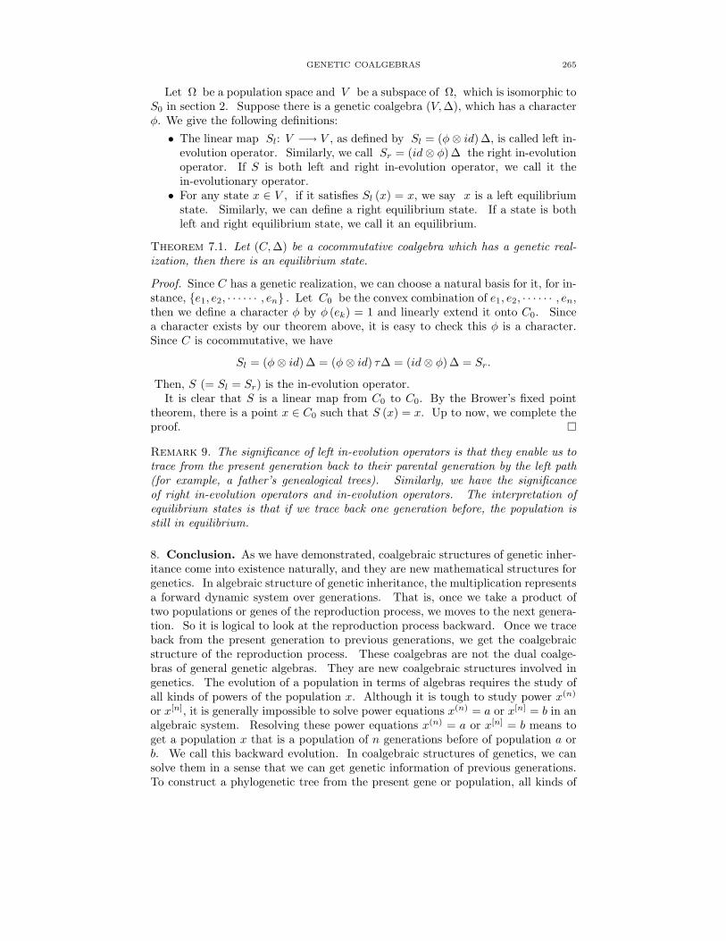
Let Ω be a population space and V be a subspace of Ω, which is isomorphic toS0 in section 2. Suppose there is a genetic coalgebra (V,∆), which has a characterφ. We give the following definitions:

• The linear map Sl: V −→ V , as defined by Sl = (φ ⊗ id) ∆, is called left in-evolution operator. Similarly, we call Sr = (id ⊗ φ) ∆ the right in-evolutionoperator. If S is both left and right in-evolution operator, we call it thein-evolutionary operator.

• For any state x ∈ V , if it satisfies Sl (x) = x, we say x is a left equilibriumstate. Similarly, we can define a right equilibrium state. If a state is bothleft and right equilibrium state, we call it an equilibrium.

Theorem 7.1. Let (C,∆) be a cocommutative coalgebra which has a genetic real-ization, then there is an equilibrium state.

Proof. Since C has a genetic realization, we can choose a natural basis for it, for in-stance, e1, e2, · · · · · · , en . Let C0 be the convex combination of e1, e2, · · · · · · , en,then we define a character φ by φ (ek) = 1 and linearly extend it onto C0. Sincea character exists by our theorem above, it is easy to check this φ is a character.Since C is cocommutative, we have

Sl = (φ ⊗ id) ∆ = (φ ⊗ id) τ∆ = (id ⊗ φ)∆ = Sr.

Then, S (= Sl = Sr) is the in-evolution operator.It is clear that S is a linear map from C0 to C0. By the Brower’s fixed point

theorem, there is a point x ∈ C0 such that S (x) = x. Up to now, we complete theproof.

Remark 9. The significance of left in-evolution operators is that they enable us totrace from the present generation back to their parental generation by the left path(for example, a father’s genealogical trees). Similarly, we have the significanceof right in-evolution operators and in-evolution operators. The interpretation ofequilibrium states is that if we trace back one generation before, the population isstill in equilibrium.

8. Conclusion. As we have demonstrated, coalgebraic structures of genetic inher-itance come into existence naturally, and they are new mathematical structures forgenetics. In algebraic structure of genetic inheritance, the multiplication representsa forward dynamic system over generations. That is, once we take a product oftwo populations or genes of the reproduction process, we moves to the next genera-tion. So it is logical to look at the reproduction process backward. Once we traceback from the present generation to previous generations, we get the coalgebraicstructure of the reproduction process. These coalgebras are not the dual coalge-bras of general genetic algebras. They are new coalgebraic structures involved ingenetics. The evolution of a population in terms of algebras requires the study ofall kinds of powers of the population x. Although it is tough to study power x(n)

or x[n], it is generally impossible to solve power equations x(n) = a or x[n] = b in analgebraic system. Resolving these power equations x(n) = a or x[n] = b means toget a population x that is a population of n generations before of population a orb. We call this backward evolution. In coalgebraic structures of genetics, we cansolve them in a sense that we can get genetic information of previous generations.To construct a phylogenetic tree from the present gene or population, all kinds of

266 J. TIAN, B. LI

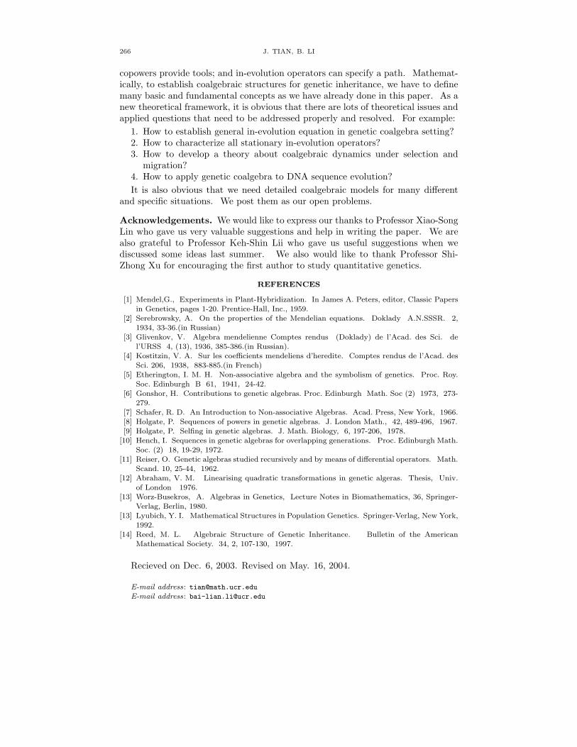
copowers provide tools; and in-evolution operators can specify a path. Mathemat-ically, to establish coalgebraic structures for genetic inheritance, we have to definemany basic and fundamental concepts as we have already done in this paper. As anew theoretical framework, it is obvious that there are lots of theoretical issues andapplied questions that need to be addressed properly and resolved. For example:

1. How to establish general in-evolution equation in genetic coalgebra setting?2. How to characterize all stationary in-evolution operators?3. How to develop a theory about coalgebraic dynamics under selection and

migration?4. How to apply genetic coalgebra to DNA sequence evolution?

It is also obvious that we need detailed coalgebraic models for many differentand specific situations. We post them as our open problems.

Acknowledgements. We would like to express our thanks to Professor Xiao-SongLin who gave us very valuable suggestions and help in writing the paper. We arealso grateful to Professor Keh-Shin Lii who gave us useful suggestions when wediscussed some ideas last summer. We also would like to thank Professor Shi-Zhong Xu for encouraging the first author to study quantitative genetics.

REFERENCES

[1] Mendel,G., Experiments in Plant-Hybridization. In James A. Peters, editor, Classic Papers

in Genetics, pages 1-20. Prentice-Hall, Inc., 1959.[2] Serebrowsky, A. On the properties of the Mendelian equations. Doklady A.N.SSSR. 2,

1934, 33-36.(in Russian)[3] Glivenkov, V. Algebra mendelienne Comptes rendus (Doklady) de l’Acad. des Sci. de

l’URSS 4, (13), 1936, 385-386.(in Russian).

[4] Kostitzin, V. A. Sur les coefficients mendeliens d’heredite. Comptes rendus de l’Acad. desSci. 206, 1938, 883-885.(in French)

[5] Etherington, I. M. H. Non-associative algebra and the symbolism of genetics. Proc. Roy.Soc. Edinburgh B 61, 1941, 24-42.

[6] Gonshor, H. Contributions to genetic algebras. Proc. Edinburgh Math. Soc (2) 1973, 273-

279.[7] Schafer, R. D. An Introduction to Non-associative Algebras. Acad. Press, New York, 1966.

[8] Holgate, P. Sequences of powers in genetic algebras. J. London Math., 42, 489-496, 1967.[9] Holgate, P. Selfing in genetic algebras. J. Math. Biology, 6, 197-206, 1978.

[10] Hench, I. Sequences in genetic algebras for overlapping generations. Proc. Edinburgh Math.

Soc. (2) 18, 19-29, 1972.[11] Reiser, O. Genetic algebras studied recursively and by means of differential operators. Math.

Scand. 10, 25-44, 1962.[12] Abraham, V. M. Linearising quadratic transformations in genetic algeras. Thesis, Univ.

of London 1976.

[13] Worz-Busekros, A. Algebras in Genetics, Lecture Notes in Biomathematics, 36, Springer-Verlag, Berlin, 1980.

[13] Lyubich, Y. I. Mathematical Structures in Population Genetics. Springer-Verlag, New York,

1992.[14] Reed, M. L. Algebraic Structure of Genetic Inheritance. Bulletin of the American

Mathematical Society. 34, 2, 107-130, 1997.

Recieved on Dec. 6, 2003. Revised on May. 16, 2004.

E-mail address: tian@math.ucr.edu

E-mail address: bai-lian.li@ucr.edu