53
RADIATIVE HEAT TRANSFER Second Edition Michael F. Modest The Pennsylvania State University COMPUTER CODES Last updated May 29, 2003 Academic Press New York San Francisco London 1
| Date post: | 12-Nov-2014 |
| Category: |
Documents |
| Upload: | edson-da-silva |
| View: | 75 times |
| Download: | 8 times |

RADIATIVE HEAT TRANSFER
Second Edition
Michael F. ModestThe Pennsylvania State University
COMPUTER CODESLast updated May 29, 2003
Academic PressNew York San Francisco London
1
2
This manual/web page contains a listing and short description of a number of computer programs thatmay be helpful to the reader of this book, and that can be downloaded from its dedicated web site, foundat http://www.academicpressbooks.com. Some of the codes are very basic and are entirely intendedto aid the reader with the solution to the problems given at the end of the more basic chapters. Some ofthe codes were born out of research, but are basic enough to aid a graduate student with more complicatedassignments or a semester project. And a few programs are so sophisticated in nature that they will be usefulonly to the practicing engineer conducting his or her own research. Finally, it is anticipated that the web sitewill be kept up-to-date and augmented once in a while. Thus, there may be a few additional programs notdescribed in this appendix.
It is a fact that most engineers have done, and still do, their programming in Fortran, and the authorof this book is no exception. It is also true that computer scientists and most commercial programmers dotheir work in C++; more importantly, the younger generation of engineers at many universities across theU.S. are now also learning C++. Since all the programs in this listing were written by the author, eitherfor research purposes or for the creation of this book, they all started their life in Fortran (older programsas Fortran77, and the later ones as Fortran90). However, as a gesture toward the C++ community, the mostbasic codes have all been converted to C++, as indicated below by the program suffix .c. If desired, allother programs are easily converted with freeware translators such asf2c (resulting in somewhat clumsy,but functional codes).
The programs are listed in order by chapter in which they first appear. More detailed descriptions,sometimes with an example, can be found on the web site. Third-party codes that are also provided at theweb site are listed at the end.
Chapter 1
bbfn.f, bbfn.cppFunctionbbfn(x) calculates the fractional blackbody emissive power, as defined by equation (1.23), wherethe argument isx= nλT with units ofµmK.
planck.f, planck.cpp, planck.exeplanck is a small stand-alone program that prompts the user for input (temperature and wavelength orwavenumber), then calculates the spectral blackbody emissive powersEbλ/T5,Ebη/T3 and the fractionalblackbody emissive powerf (λT).
Chapters 2 and 3
fresnel.f, fresnel.cppSubroutinefresnel(n,k,th,rhos,rhop,rho) calculates Fresnel reflectances from equation (2.112).Input: n (= n) andk (= k) are real and imaginary parts of the complex index of refraction, andth (= θ) isthe off-normal angle of incidence (in radians).Output: rhos (= ρ⊥) andrhop (= ρ‖) are perpendicular and parallel-polarized reflectance, respectively,while rho (= ρ) is the unpolarized reflectance.
Chapter 3
emdiel.f90, emdiel.cpp
Functionemdiel(n) calculates the unpolarized, spectral, hemispherical emissivity of an optical surface ofa dielectric material from equation (3.82).Input: n (= n) refractive index of dielectric.

3
emmet.f90, emmet.cpp
Functionemmet(n,k) calculates the unpolarized, spectral, hemispherical emissivity of an optical surface ofa metallic material from equation (3.77).Input: n (= n) andk (= k) are the real and imaginary parts of the metal’s complex index of refraction.
callemdiel.f90, callemdiel.cpp, callemdiel.exeProgramcallemdiel is a stand-alone front end for functionemdiel, prompting for input (refractive indexn) and returning the unpolarized, spectral, hemispherical as well as normal emissivities.
callemmet.f90, callemmet.cpp, callemmet.exeProgramcallemmet is a stand-alone front end for functionemmet, prompting for input (complex index ofrefractionn, k) and returning the unpolarized, spectral, hemispherical as well as normal emissivities.
dirreflec.f, dirreflec.cpp, dirreflec.exe
Programdirrecflec is a stand-alone front end for subroutinefresnel, calculating reflectivities for vari-ous incidence angles. The user is prompted to input the complex index of refraction,n andk, and the (equal)spacing of incidence angles∆θ (in degrees); the program then returns perpendicular polarized, parallel po-larized, and unpolarized reflectivities, as well as unpolarized emissivities.
totem.f90, totem.cppProgramtotem is a routine to evaluate the total, directional or hemispherical emittance or absorptance ofan opaque material, based on an array of spectral data, by 10-point Gaussian quadrature.Input (by changing data in the heading of functionemlcl(y)):N = number of data points for spectral emittance,nrefr = refractive index of adjoining material (nrefr=1 for vacuum and gases),T = temperature of material (for total emittance), or of gray irradiating source (for total absorp-
tance), in K,lambda(N) = N distinct wavelengths in ascending order, for which the spectral emittance is given, inµm,eps(N) = N corresponding spectral emittances.Output (printed to screen):emitt = total directional or hemispherical emittance or absorptance.Case 1: Total, directional emittance (eps contains spectral, directional values at temperatureT):From equation (3.8)
ε′(T, s) =1
n2σT4
∫ ∞
0ε′λ(λ,T, s)Ebλ(T) dλ
=
∫ 1
0ε′λ(λ( f ),T, s
)d f, (CC-1)
where, from equation (1.23)
f (nλT) =∫ λ
0
Ebλdλ
n2σT4. (CC-2)
In order to write equation (CC-1) in terms of blackbody fractionf , wavelength must be known as a functionof f (for givenn andT), i.e., equation (CC-2) must be inverted. The 10 values of (nλT), corresponding tothe 10 Gaussian quadrature pointsfi(nλT) have been precalculated (using functionbbfn) and are stored inarrayy(i). The total emittance is then calculated by expressing equation (CC-1) in quadrature form, or
ε′(T, s) '10∑i=1
ε′λ(λi ,T, s)wi , (CC-3)
whereλi = yi/nT, (CC-4)

4
and thewi are Gaussian quadrature weights. This necessitates thatε′λ must be known at very specific wave-lengths, that are not ordinarily part of the given array. The “correct” value forε′λ is evaluated by linearinterpolation between array values, assumingε′λ = const= eps(1) for λi <lambda(1), andε′λ = const=eps(N) for λi >lambda(N).Case 2:Total, hemispherical emittance (eps contains spectral, hemispherical values at temperatureT):From equation (3.10)
ε(T) =1
n2σT4
∫ ∞
0ελ(λ,T)Ebλ dλ =
∫ 1
0ελ(λ( f ),T
)d f
'
10∑i=1
ελ(λi ,T)wi . (CC-5)
Thus, the calculation is identical to Case 1.Case 3:Total, directional absorptance (eps contains spectral, directional values at the surface temperatureTs, irradiation is assumed to come from a gray source at temperatureT).From equations (3.23) and (3.31)
α′(Ts,T, s) =1
n2σT4
∫ ∞
0ε′λ(λ,T, s)Ebλ(T) dλ
=
∫ 1
0ε′λ(λ( f ),Ts
)d f '
10∑i=1
ε′λ(λi ,Ts)wi , (CC-6)
and the calculation is again identical.Case 4:Total, hemispherical absorptance (eps contains spectral, hemispherical values at surface tempera-tureTs; irradiation is assumed to be gray and diffuse with source temperatureT).Then, from equations (3.27) and (3.31)
α(Ts,T) =1
n2σT4
∫ ∞
0ελ(λ,Ts)Ebλ(T) dλ
=
∫ 1
0ελ(λ( f ),Ts
)d f '
10∑i=1
ελ(λi ,Ts)wi . (CC-7)
ExamplesTwo examples have been programmed intototem (or, rather, functionemlcl):
1.: The material of Problem 3.1, with a step function in spectral emittance of
ελ =
0.5, λ < 5µm,0.3, λ > 5µm,
and a temperature ofT = 500 K. For parta) nrefr=1.0, and forb) nrefr=2.0 (implemented here)This results inemitt=0.3435 for a) andemitt=0.4296 for b).
2.: Aluminum oxide, as given in Fig. 1-13, discretized into eight equally-spaced values (commented out asgiven here). For temperature ofT = 500 K andnrefr=1.0 this results inemitt=0.7494.

5
Chapter 4 and Appendix D
view.f90, view.cppA function to evaluate any of the 51 view factors given in Appendix D.Input:NO = view factor number, 1≤ NO ≤ 51, as given in Appendix D,NARG = number of arguments required for view factor,ARG = vector of orderNARG containing the arguments in alphabetical order (Greek characters follow-
ing the Roman alphabet).
For example, for view factor 14, we haveNO=14, NARG=3 andARG=(h, l, r). Upon return the function returnsFi− j (except for the infinitesimal view factors 1–9, in which casedFd1−d2/dX is returned, withdX thenondimensional dimension ofdA2).
parlplates.f90, parlplates.cppContains functionPARLPLTF(X1,X2,X3,Y1,Y2,Y3,Z) to evaluate the view factor between two displacedparallel plates, as given by equation (4.41).
Input:
X1 = Dimensionx1 as given in adjacent sketch (length units)X2 = Dimensionx2 as given in adjacent sketch (length units)X3 = Dimensionx3 as given in adjacent sketch (length units)Y1 = Dimensiony1 as given in adjacent sketch (length units)Y2 = Dimensiony2 as given in adjacent sketch (length units)Y3 = Dimensiony3 as given in adjacent sketch (length units)Z = Dimensionc as given in adjacent sketch (length units)
y
A1
0 x1 x2x3
x
y2
y1
y3
A2
c
perpplates.f90, perpplates.cppContains functionPERPPLTF(X1,X2,Y1,Y2,Z1,Z2,Z3) to evaluate the view factor between two displacedperpendicular plates, as given by equation (4.40).
Input:
X1 = Dimensionx1 as given in adjacent sketch (length units)X2 = Dimensionx2 as given in adjacent sketch (length units)Y1 = Dimensiony1 as given in adjacent sketch (length units)Y2 = Dimensiony2 as given in adjacent sketch (length units)Z1 = Dimensionz1 as given in adjacent sketch (length units)Z2 = Dimensionz2 as given in adjacent sketch (length units)Z3 = Dimensionz3 as given in adjacent sketch (length units)
y
y2
y1
0
x1 x2x
z3
z2
z1
A2
A1
z
A1
viewfactors.f90, viewfactors.cpp, viewfactors.exeA stand-alone front end to functionsview, parlplates andperpplates. The user is prompted to inputconfiguration number and arguments; the program then returns the requested view factor.
Chapter 5
graydiff.f90, graydiff.cpp:Subroutinegraydiff provides the solution to equation (5.38) for an enclosure consisting ofN gray-diffusesurfaces. For each surface the area, emittance, external irradiation and either heat flux or temperature must
6
be specified. In addition, the upper triangle of the view factor matrix must be provided (Fi− j ; i = 1,N;j = i,N). For closed configurations, the diagonal view factorsFi−i are not required, since they can becalculated from the summation rule. The remaining view factors are calculated from reciprocity. On output,the program provides all view factors, and temperatures and radiative heat fluxes for all surfaces.Input:N = number of surfaces in enclosureiclsd = closed or open configuration identifier
iclsd= 1: configuration is closed; diagonalFi−i evaluated from summation ruleiclsd, 1: configuration has openings;Fi−i must be specified
A(N) = vector containing surface areas, [m2]EPS(N) = vector containing surface emittancesHO(N) = vector containing external irradiation, in [W/m2]F(N,N) = vector containing view factors; on input onlyFi− j with j > i (iclsd=1) or j ≥ i (iclsd, 1)
are required; remainder are calculatedID(N) = vector containing surface identifier:
ID=0: surface heat flux is specified, in [W/m2]ID=1: surface temperature is specified, in [K]
PIN(N) = vector containing surface emissive powers (id=1) and fluxes (id=2)Output:POUT(N) = vector containing unknown surface fluxes (for surfaces withid=1) and emissive powers (for
surfaces withid=0)
graydiffxch.f90, graydiffxch.cppProgramgraydiffxch is a front end for subroutinegraydiff, generating the necessary input parametersfor a three-dimensional variation to Example 5.4 (making the four surfaces of finite length`, and introducingfront and back surfacesA5 andA6, both at the same conditions as the left and right sides, i.e.,T5 = T6 =
600 K andε5 = ε6 = 0.8), primarily view factors calculated by calls to functionview. This program may beused as a starting point for more involved radiative exchange problems.
Chapter 6
graydifspec.f90, graydifspec.cppSubroutinegraydifspec provides the solution to equation (6.23) for an enclosure consisting ofN diffuselyemitting surfaces with diffuse and specular reflectance components. For each surface the area, emittance,external irradiation and either heat flux or temperature must be specified. In addition, the upper triangle ofthe view factor matrix must be provided (Fs
i− j ; i = 1,N; j = i,N). For closed configurations, the diagonalview factorsFs
i−i are not required, since they can be calculated from the summation rule. The remaining viewfactors are calculated from reciprocity. On output, the program provides all view factors, and temperaturesand radiative heat fluxes for all surfaces.Input:N = number of surfaces in enclosureiclsd = closed or open configuration identifier
iclsd= 1: configuration is closed; diagonalFsi−i evaluated from summation rule
iclsd, 1: configuration has openings;Fsi−i must be specified
A(N) = vector containing surface areas, [m2]EPS(N) = vector containing surface emittancesRHOs(N) = vector containing surface specular reflectance componentsHOs(N) = vector containing external irradiation, in [W/m2]

7
Fs(N,N) = vector containing view factors; on input onlyFsi− j with j > i (iclsd=1) or j ≥ i (iclsd, 1)
are required; remainder are calculatedID(N) = vector containing surface identifier:
ID=0: surface heat flux is specified, in [W/m2]ID=1: surface temperature is specified, in [K]
PIN(N) = vector containing surface emissive powers (id=1) and fluxes (id=2)Output:POUT(N) = vector containing unknown surface fluxes (for surfaces withid=1) and emissive powers (for
surfaces withid=0)
grspecxch.f90, grspecxch.cppProgramgrspecxch is a front end for subroutinegraydifspec, generating the necessary input parametersfor a three-dimensional variation to Example 6.7 (making the four surfaces of finite length`, and introducingfront and back surfacesA5 andA6, both diffusely reflecting at the same conditions as the left and right sides,i.e., T5 = T6 = 600 K andε5 = ε6 = 0.8), primarily view factors calculated by calls to functionview. Thisprogram may be used as a starting point for more involved radiative exchange problems.
Chapter 7
semigray.f90, semigray.cpp, semigraydf.f90, semigraydf.cppSubroutinesemigray provides the solution to equations (7.5) for an enclosure consisting ofN diffuselyemitting surfaces with diffuse and specular reflectance components, considering two spectral ranges (onefor external irradiation, one for emission). For each surface the area, emittance and specular reflectance(two values each), external irradiation and either heat flux or temperature must be specified. In addition, theupper triangle of the view factor matrix must be provided for both spectral ranges (Fs
i− j ; i = 1,N; j = i,N).For closed configurations, the diagonal view factorsFs
i−i are not required, since they can be calculated fromthe summation rule. The remaining view factors are calculated from reciprocity. On output, the programprovides all view factors, and temperatures and radiative heat fluxes for all surfaces.Input:N = number of surfaces in enclosureiclsd = closed or open configuration identifier
iclsd= 1: configuration is closed; diagonalFsi−i evaluated from summation rule
iclsd, 1: configuration has openings;Fsi−i must be specified
A(N) = vector containing surface areas, [m2]EPS(2,N) = vector containing surface emittances for 2 spectral rangesRHOs(2,N) = vector containing surface specular reflectance components for 2 spectral rangesHOs(N) = vector containing external irradiation, in [W/m2]Fs(2,N,N) = vector containing view factors for 2 spectral ranges; on input onlyFs
i− j with j > i (iclsd=1)or j ≥ i (iclsd, 1) are required; remainder are calculated
ID(N) = vector containing surface identifier:ID=0: surface heat flux is specified, in [W/m2]ID=1: surface temperature is specified, in [K]
PIN(N) = vector containing surface emissive powers (id=1) and fluxes (id=2)Output:POUT(N) = vector containing unknown surface fluxes (for surfaces withid=1) and emissive powers (for
surfaces withid=0)
Subroutinesemigraydf is a simplified version of subroutinesemigray by assuming all surfaces to bediffuse, and input is changed by requiringHO(N) andF(N,N) (and no reflectance) instead ofRHOs(2,N),HOs(N) andFs(2,N,N) (note that diffuse view factors do not depend on reflectance properties).
8
semigrxch.f90, semigrxch.cpp, semigrxchdf.f90, semigrxchdf.cppProgramsemigrxch is a front end for subroutinesemigray providing the necessary input for Example 7.1,primarily view factors calculated by calls to functionview; similarly, programsemigrxchdf is a front endfor subroutinesemigraydf. These programs may be used as a starting point for more involved radiativeexchange problems.
bandapp.f90, bandapp.cpp, bandappdf.f90, bandappdf.cppSubroutinebandapp provides the solution to equations (7.6) for an enclosure consisting ofN diffuselyemitting surfaces with diffuse and specular reflectance components, consideringM spectral bands. For eachsurface the area, emittance, specular reflectance and external irradiation (one value for each spectral band),and either heat flux or temperature must be specified. In addition, the upper triangle of the view factor matrixmust be provided for each spectral band (Fs
i− j ; i = 1,N; j = i,N). For closed configurations, the diagonalview factorsFs
i−i are not required, since they can be calculated from the summation rule. The remaining viewfactors are calculated from reciprocity. On output, the program provides all view factors, and temperaturesand radiative heat fluxes for all surfaces.Input:M = number of spectral bandsN = number of surfaces in enclosureiclsd = closed or open configuration identifier
iclsd= 1: configuration is closed; diagonalFsi−i evaluated from summation rule
iclsd, 1: configuration has openings;Fsi−i must be specified
A(N) = vector containing surface areas, [m2]EPS(M,N) = matrix containing surface emittances forM spectral rangesRHOs(M,N) = matrix containing surface specular reflectance components forM spectral rangesHOs(M,N) = matrix containing external irradiation forM spectral ranges, in [W/m2]Fs(M,N,N) = matrix containing view factors forM spectral ranges; on input onlyFs
i− j with j > i(iclsd=1) or j ≥ i (iclsd, 1) are required; remainder are calculated
ID(N) = vector containing surface identifier:ID=0: surface heat flux is specified, in [W/m2]ID=1: surface temperature is specified, in [K]
q(N) = vector containing known surface fluxes (only for surfaces withid=2)T(N) = vector containing known surface temperatures (only for surfaces withid=1)Output:q(N) = vector containing known surface fluxes (for all surfaces)T(N) = vector containing known surface temperatures (for all surfaces)
Subroutinebandappdf is a simplified version of subroutinebandapp by assuming all surfaces to be dif-fuse, and input is changed by requiringHO(M,N) andF(N,N) (and no reflectance) instead ofRHOs(M,N),HOs(M,N) andFs(M,N,N) (note that diffuse view factors do not depend on reflectance properties).
bandmxch.f90, bandmxch.cpp, bandmxchdf.f90, bandmxchdf.cppProgrambandmxch is a front end for subroutinebandapp providing the necessary input for Example 7.2,primarily view factors calculated by calls to functionview; similarly, programbandmxchdf is a front endfor subroutinebandappdf. These programs may be used as a starting point for more involved radiativeexchange problems.
Chapter 10
voigt.f
Fortran77 subroutinevoigt(S,bL,bD,deta,keta) calculates the spectral absorption coefficient for a

9
Voigt-shaped line based on the fast algorithm by Humlıcek [1].Input:S = is the line intensityS, in cm−2,bL = is the Lorentz line widthbL, in cm−1,bD = is the Doppler line widthbD, in cm−1,deta = is the spectral distance∆η away from the line center, at whichκη is to be evaluated.Output:keta = is the spectral absorption coefficient of the Voigt lineκη at η = η0 ± ∆η, whereη0 is the
wavenumber of the line center.nbkdist.f90
Programnbkdist is a Fortran90 code to calculate narrow bandk-distributions for a number of temperaturesand a number of wavenumber ranges, for a gas mixture containing CO2, H2O, CH4 and soot. The spectralabsorption coefficient is either calculated directly from the HITRAN or HITEMP databases, or is suppliedby the user.Input:Tmin = minimum temperature for which ak-distribution is to be calculated, in K,Tmax = maximum temperature for which ak-distribution is to be calculated, in K,numT = number of different temperatures to be considered; equally spaced betweenTmin andTmax,P = total pressure of gas mixture, bar,xmfr(3) = mole fraction vector;xmfr(1)= mole fraction of CO2, xmfr(2)= mole fraction of H2O,
xmfr(3)= mole fraction of CH4,fvsoot = volume fraction of soot,nsoot,
ksoot
= complex index of refraction for the soot; its absorption coefficient is assumed linear inwavenumber, using equation (11.116),
wvnm b = minimum wavenumber considered, cm−1,wvnm e = maximum wavenumber considered, cm−1,wvnmbuf = line wing influence of spectral lines centered in the wavenumber rangewvnmbuf cm−1 below
wvnm b and abovewvnm e are considered in the absorption coefficient calculation, cm−1,wvnmst = wavenumber step (equally spaced) with which the absorption coefficient for the mixture is
calculated from the HITRAN or HITEMP database, cm−1,kdrnge = wavenumber range for individualk-distributions;wvnm e-wvnm b should be an integer multi-
ple of kdrnge, in cm−1,n pwrk = number of differentk-bin values considered in the construction of thek-distribution,pwr = exponent fork-bin values spacing:k-bins are equally spaced inkpwr betweenkmin (=mini-
mumk to be considered) andkmax (=maximum absorption coefficient across spectrum).nq = number of quadrature points for radiative calculations, i.e., the number of RTE evaluations to
be performed before spectral integration (over cumulativek-distributiong),iwr = absorption coefficient switch:iwr=0 to make a single complete run, i.e., evaluatingκη from HI-
TRAN or HITEMP (without storing them), followed by generation ofk-distributions,irw=1same, but absorption coefficient is stored for future use, andiwr=2: precalculated absorptioncoefficients are read in andk-distributions are generated.
ipl = linear vs. pressure-based absorption coefficient switch:ipl=0: calculate linear absorption coefficient, in cm−1
ipl=1: calculate pressure-based absorption coefficient (allowed only for single absorbinggas!), in cm−1 bar−1; if the pressure-based absorption coefficient for a dilute gas is desired, setxmfr=1.d-3 (=0.1%)
ipr = output switch: see under outputOutput:
ipr=0: For each of thenumkd=wvnm e-wvnm b/kdrnge narrow band ranges only thenq quadrature points,

10
weights, andk(T, g) (for all temperatures) are printed: the first line of the output file, callednbkvsgq.dat
by default, contains the first and last wavenumbers of the first narrow band range, followed bynq
lines containinggq (the i-th quadrature point),wq (the i-th quadrature weight), andnumT values ofkq [= k(Tj , gi); one for each temperatureTj ]. This is followed by a line containing the first and lastwavenumbers of the second narrow band range, etc.
ipr=1: Besides the output foripr=0 a second output file is prepared with the completek-distributioninformation, i.e., for each narrow band and each temperature alln pwrk values ofk, f and g areprinted: the first line of the output file, callednbkvsg.dat by default, contains the first temperatureand first and last wavenumbers of the first narrow band range, followed byn pwrk-1 lines containingk (the i-th k-bin value),ff [its k-distribution valuef (k)], andgg [its cumulativek-distribution valueg(k)]. This is followed by a line containing the second temperature and first and last wavenumbers ofthe first narrow band range, etc., looping over all temperatures and narrow band ranges.
ipr=2: Only the completek-distribution information is printed, i.e., only output filenbkvsg.dat is gener-ated.
Example:We consider a set of narrow bandk-distributions for a linear absorption coefficient (ipl=0) of pure CO2,for a mole fraction of 10% (xmfr(3)=(/0.1d0,0.d0,0.d0/)). The absorption coefficient is calculated inthis run (iwr=1), and is stored in fileC:\absco\absctmp.dat (for a wavenumber range from 2320 cm−1
to 2380 cm−1, but also considering lines centered at wavenumbers as low as 2315 cm−1 and as high as2385 cm−1, wvnmbuf=5.) with a δη = 0.001 cm−1. We will calculate thek-distributions for 4 temperatures,equally spaced betweenTmin = 300 K andTmax = 1200 K (numT=4): this results in the 4 temperatures of300 K, 600 K, 900 K and 1200 K. Eachk-distribution will be over a range of∆η = 10 cm−1 wavenumbers(kdrnge=10.), i.e., there will be 6 narrow bands. We will use 500k-bins (n_pwrk=500) withpwr=0.1 (thisspreads thek-bins over many orders of magnitude, but places more and more bins into large magnitudes;see output file). We also setklmin=10−9 (cm−1), i.e., we will consider absorption coefficient contributionsas small as 10−9 cm−1. Finally, we setipr=1 andnq=10, i.e., besides truncatedk-distributions ready-madefor numerical quadrature, using 10 quadrature points, we want to also print to file the fullk-distributions.The top of the program with input parameters, therefore, looks like this:MODULE Key
IMPLICIT NONE
!HITRAN/HITEMP DATABASE
INTEGER :: lu
INTEGER,PARAMETER :: rows=1400000
DOUBLE PRECISION,PARAMETER :: wvnm_b=2320.d0,wvnm_e=2380.d0,wvnmbuf=5.d0,wvnmst=0.001d0
DOUBLE PRECISION :: data(rows,6),wvnm_l=wvnm_b-wvnmbuf,wvnm_r=wvnm_e+wvnmbuf
END MODULE Key
PROGRAM Main
USE Key
! Input parameters
INTEGER,PARAMETER :: numT=4,n_pwrk=500,nq=10,iwr=1,ipl=0,ipr=1
DOUBLE PRECISION,PARAMETER :: P=1.d0,Tmin=300d0,Tmax=1200d0,kdrnge=10.
DOUBLE PRECISION,PARAMETER :: xmfr(3)=(/0.10d0,0.00d0,0.d0/),pwr=0.1d0,klmin=1.d-9
DOUBLE PRECISION,PARAMETER :: fvsoot=0.d-6,nsoot=1.89d0,ksoot=0.92d0
where we have changed the values forwvnm_b, wvnm_e, wvnmst, numT, n_pwrk, iwr, ipr, nq,Tmin, Tmax andxmfr to fit our needs. Also, in this simulation we have set file names as! Open output files
IF(ipr<2) OPEN(7,FILE=’nbkvsgqco2.dat’,STATUS=’unknown’)
IF(ipr>0) OPEN(8,FILE=’nbkvsgco2.dat’,STATUS=’unknown’)
! File containing absorption coefficient
IF(iwr>0) OPEN(9,FILE=’C:\absco\absctmp.dat’,STATUS=’unknown’)
11
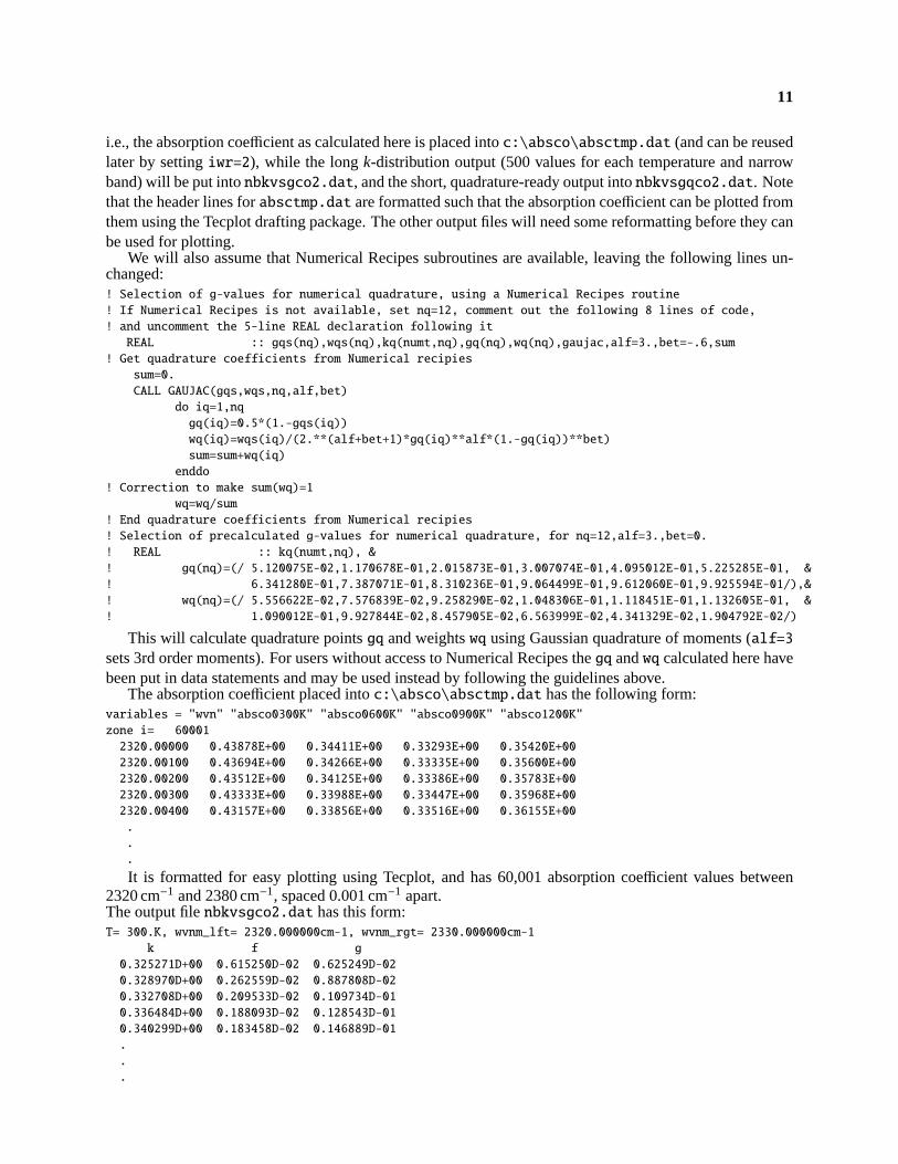
i.e., the absorption coefficient as calculated here is placed intoc:\absco\absctmp.dat (and can be reusedlater by settingiwr=2), while the longk-distribution output (500 values for each temperature and narrowband) will be put intonbkvsgco2.dat, and the short, quadrature-ready output intonbkvsgqco2.dat. Notethat the header lines forabsctmp.dat are formatted such that the absorption coefficient can be plotted fromthem using the Tecplot drafting package. The other output files will need some reformatting before they canbe used for plotting.
We will also assume that Numerical Recipes subroutines are available, leaving the following lines un-changed:! Selection of g-values for numerical quadrature, using a Numerical Recipes routine
! If Numerical Recipes is not available, set nq=12, comment out the following 8 lines of code,
! and uncomment the 5-line REAL declaration following it
REAL :: gqs(nq),wqs(nq),kq(numt,nq),gq(nq),wq(nq),gaujac,alf=3.,bet=-.6,sum
! Get quadrature coefficients from Numerical recipies
sum=0.
CALL GAUJAC(gqs,wqs,nq,alf,bet)
do iq=1,nq
gq(iq)=0.5*(1.-gqs(iq))
wq(iq)=wqs(iq)/(2.**(alf+bet+1)*gq(iq)**alf*(1.-gq(iq))**bet)
sum=sum+wq(iq)
enddo
! Correction to make sum(wq)=1
wq=wq/sum
! End quadrature coefficients from Numerical recipies
! Selection of precalculated g-values for numerical quadrature, for nq=12,alf=3.,bet=0.
! REAL :: kq(numt,nq), &
! gq(nq)=(/ 5.120075E-02,1.170678E-01,2.015873E-01,3.007074E-01,4.095012E-01,5.225285E-01, &
! 6.341280E-01,7.387071E-01,8.310236E-01,9.064499E-01,9.612060E-01,9.925594E-01/),&
! wq(nq)=(/ 5.556622E-02,7.576839E-02,9.258290E-02,1.048306E-01,1.118451E-01,1.132605E-01, &
! 1.090012E-01,9.927844E-02,8.457905E-02,6.563999E-02,4.341329E-02,1.904792E-02/)
This will calculate quadrature pointsgq and weightswq using Gaussian quadrature of moments (alf=3
sets 3rd order moments). For users without access to Numerical Recipes thegq andwq calculated here havebeen put in data statements and may be used instead by following the guidelines above.
The absorption coefficient placed intoc:\absco\absctmp.dat has the following form:variables = "wvn" "absco0300K" "absco0600K" "absco0900K" "absco1200K"
zone i= 60001
2320.00000 0.43878E+00 0.34411E+00 0.33293E+00 0.35420E+00
2320.00100 0.43694E+00 0.34266E+00 0.33335E+00 0.35600E+00
2320.00200 0.43512E+00 0.34125E+00 0.33386E+00 0.35783E+00
2320.00300 0.43333E+00 0.33988E+00 0.33447E+00 0.35968E+00
2320.00400 0.43157E+00 0.33856E+00 0.33516E+00 0.36155E+00
.
.
.
It is formatted for easy plotting using Tecplot, and has 60,001 absorption coefficient values between2320 cm−1 and 2380 cm−1, spaced 0.001 cm−1 apart.The output filenbkvsgco2.dat has this form:T= 300.K, wvnm_lft= 2320.000000cm-1, wvnm_rgt= 2330.000000cm-1
k f g
0.325271D+00 0.615250D-02 0.625249D-02
0.328970D+00 0.262559D-02 0.887808D-02
0.332708D+00 0.209533D-02 0.109734D-01
0.336484D+00 0.188093D-02 0.128543D-01
0.340299D+00 0.183458D-02 0.146889D-01
.
.
.
12
0.277993D+02 0.340523D-03 0.997833D+00
0.280016D+02 0.402225D-03 0.998235D+00
0.282052D+02 0.521735D-03 0.998757D+00
0.284102D+02 0.124290D-02 0.100000D+01
T= 600.K, wvnm_lft= 2320.000000cm-1, wvnm_rgt= 2330.000000cm-1
k f g
0.187475D+00 0.525121D-02 0.535120D-02
0.189577D+00 0.199556D-02 0.734676D-02
0.191700D+00 0.138701D-02 0.873377D-02
.
.
.
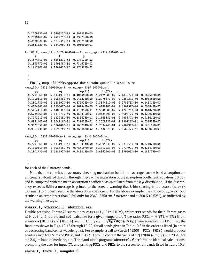
Finally, output filenbkvsgqco2.dat contains quadraturek-values as:wvnm_lft= 2320.000000cm-1, wvnm_rgt= 2330.000000cm-1
gq wq kq(T1) kq(T2) ...
0.729136D-01 0.813193D-01 0.400407D+00 0.242578D+00 0.183572D+00 0.160547D+00
0.165015D+00 0.108536D+00 0.541222D+00 0.297547D+00 0.226229D+00 0.204381D+00
0.280173D+00 0.128592D+00 0.672925D+00 0.335421D+00 0.278275D+00 0.240816D+00
0.410404D+00 0.139547D+00 0.867542D+00 0.418648D+00 0.336797D+00 0.295848D+00
0.546441D+00 0.140538D+00 0.118950D+01 0.584868D+00 0.422875D+00 0.361822D+00
0.678556D+00 0.131471D+00 0.163219D+01 0.902429D+00 0.560377D+00 0.425924D+00
0.797291D+00 0.112988D+00 0.286678D+01 0.156588D+01 0.795057D+00 0.518610D+00
0.894140D+00 0.864116D-01 0.739453D+01 0.262995D+01 0.130120D+01 0.731875D+00
0.962165D+00 0.536406D-01 0.168294D+02 0.783404D+01 0.286791D+01 0.123165D+01
0.996473D+00 0.169570D-01 0.268487D+02 0.142687D+02 0.658947D+01 0.326066D+01
wvnm_lft= 2330.000000cm-1, wvnm_rgt= 2340.000000cm-1
gq wq kq(T1) kq(T2) ...
0.729136D-01 0.813193D-01 0.716314D+00 0.299593D+00 0.223759D+00 0.171072D+00
0.165015D+00 0.108536D+00 0.788507D+00 0.371208D+00 0.277792D+00 0.221426D+00
0.280173D+00 0.128592D+00 0.943415D+00 0.436240D+00 0.339969D+00 0.280705D+00
.
.
.
for each of the 6 narrow bands.Note that the code has an accuracy-checking mechanism built in: an average narrow band absorption co-
efficient is calculated directly through line-by-line integration of the absorption coefficient, equation (10.50),and is compared with the mean absorption coefficient as calculated from thek-g-distribution. If the discrep-ancy exceeds 0.5% a message is printed to the screen, warning thatk-bin spacing is too coarse (n_pwrktoo small) to properly resolve the absorption coefficient. For the above example, the choice ofn_pwrk=500results in an error larger than 0.5% only for 2340–2350 cm−1 narrow band at 300 K (0.52%), as indicated bythe warning message.
wbmxxx.f, wbmxxxcl.f, wbmxxxcl.exe
Double precision Fortran77 subroutineswbmxxx(T,PSIr,PHIr), wherexxx stands for the different gasesh20, co2, ch4, co, no andso2, calculate for a given temperatureT the ratiosPSIr = Ψ∗(T)/Ψ∗(T0) [fromequations (10.111) and (10.114)] andPHIr = γ/γ0 =
√T0/TΦ(T)/Φ(T0) [from equation (10.115)], i.e., the
functions shown in Figs. 10-18 through 10-20, for all bands given in Table 10.3 in the order as listed (in orderof decreasing band center wavelengths). For example, a call towbmch4(1200.,PSIr,PHIr)would produce4 values each forPSIr andPHIr, andPSIr(3)would contain the value ofΨ∗(1200K)/Ψ∗(T0) = 1.29540 forthe 2.4µm band of methane, etc. The stand-alone programswbmxxxcl.f perform the identical calculations,prompting the user for input (T), and printingPSIr andPHIr to the screen for all bands listed in Table 10.3.
emwbm.f, ftwbm.f, wangwbm.f
13
Double precision Fortran77 functions to calculate the nondimensional total band absorptanceA∗ from theEdwards and Menard model, Table 10.2 (emwbm(tau,beta)), the Felske and Tien model, equation (10.124)(ftwbm(tau,beta)), and the Wang model, equation (10.126) (wangwbm(tau,beta)).
wbmodels.f, wbmodels.exe
Stand-alone double precision Fortran77 front end for the functionsemwbm, ftwbm andwangwbm; the useris prompted to inputtau (= τ0, optical thickness at band center) andbeta (= β, overlap parameter); thenondimensional total band absorptanceA∗ is printed to the screen, as calculated from three band models(Edwards and Menard, Felske and Tien, and Wang models).
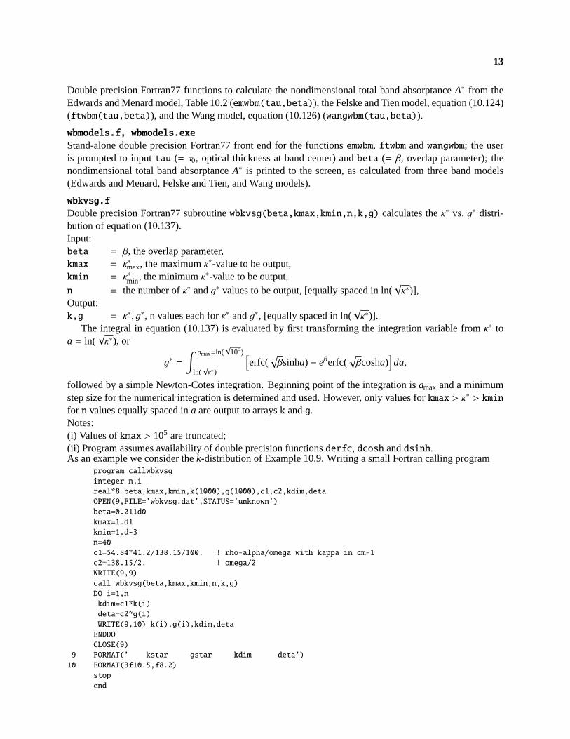
wbkvsg.f
Double precision Fortran77 subroutinewbkvsg(beta,kmax,kmin,n,k,g) calculates theκ∗ vs. g∗ distri-bution of equation (10.137).Input:beta = β, the overlap parameter,kmax = κ∗max, the maximumκ∗-value to be output,kmin = κ∗min, the minimumκ∗-value to be output,n = the number ofκ∗ andg∗ values to be output, [equally spaced in ln(
√κ∗)],
Output:k,g = κ∗, g∗, n values each forκ∗ andg∗, [equally spaced in ln(
√κ∗)].
The integral in equation (10.137) is evaluated by first transforming the integration variable fromκ∗ toa = ln(
√κ∗), or
g∗ =
∫ amax=ln(√
105)
ln(√κ∗)
[erfc(
√βsinha) − eβerfc(
√βcosha)
]da,
followed by a simple Newton-Cotes integration. Beginning point of the integration isamax and a minimumstep size for the numerical integration is determined and used. However, only values forkmax > κ∗ > kmin
for n values equally spaced ina are output to arraysk andg.Notes:(i) Values ofkmax > 105 are truncated;(ii) Program assumes availability of double precision functionsderfc, dcosh anddsinh.As an example we consider thek-distribution of Example 10.9. Writing a small Fortran calling program
program callwbkvsg
integer n,i
real*8 beta,kmax,kmin,k(1000),g(1000),c1,c2,kdim,deta
OPEN(9,FILE=’wbkvsg.dat’,STATUS=’unknown’)
beta=0.211d0
kmax=1.d1
kmin=1.d-3
n=40
c1=54.84*41.2/138.15/100. ! rho-alpha/omega with kappa in cm-1
c2=138.15/2. ! omega/2
WRITE(9,9)
call wbkvsg(beta,kmax,kmin,n,k,g)
DO i=1,n
kdim=c1*k(i)
deta=c2*g(i)
WRITE(9,10) k(i),g(i),kdim,deta
ENDDO
CLOSE(9)
9 FORMAT(’ kstar gstar kdim deta’)
10 FORMAT(3f10.5,f8.2)
stop
end
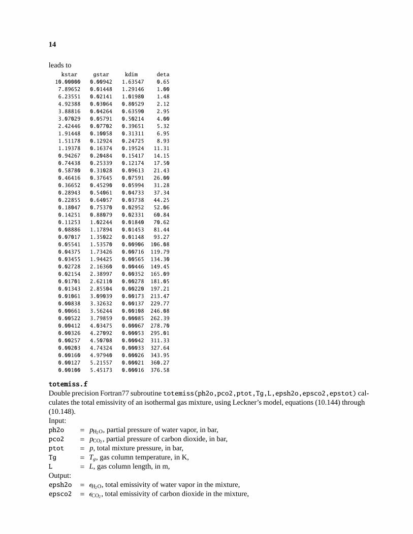
14
leads tokstar gstar kdim deta
10.00000 0.00942 1.63547 0.65
7.89652 0.01448 1.29146 1.00
6.23551 0.02141 1.01980 1.48
4.92388 0.03064 0.80529 2.12
3.88816 0.04264 0.63590 2.95
3.07029 0.05791 0.50214 4.00
2.42446 0.07702 0.39651 5.32
1.91448 0.10058 0.31311 6.95
1.51178 0.12924 0.24725 8.93
1.19378 0.16374 0.19524 11.31
0.94267 0.20484 0.15417 14.15
0.74438 0.25339 0.12174 17.50
0.58780 0.31028 0.09613 21.43
0.46416 0.37645 0.07591 26.00
0.36652 0.45290 0.05994 31.28
0.28943 0.54061 0.04733 37.34
0.22855 0.64057 0.03738 44.25
0.18047 0.75370 0.02952 52.06
0.14251 0.88079 0.02331 60.84
0.11253 1.02244 0.01840 70.62
0.08886 1.17894 0.01453 81.44
0.07017 1.35022 0.01148 93.27
0.05541 1.53570 0.00906 106.08
0.04375 1.73426 0.00716 119.79
0.03455 1.94425 0.00565 134.30
0.02728 2.16360 0.00446 149.45
0.02154 2.38997 0.00352 165.09
0.01701 2.62110 0.00278 181.05
0.01343 2.85504 0.00220 197.21
0.01061 3.09039 0.00173 213.47
0.00838 3.32632 0.00137 229.77
0.00661 3.56244 0.00108 246.08
0.00522 3.79859 0.00085 262.39
0.00412 4.03475 0.00067 278.70
0.00326 4.27092 0.00053 295.01
0.00257 4.50708 0.00042 311.33
0.00203 4.74324 0.00033 327.64
0.00160 4.97940 0.00026 343.95
0.00127 5.21557 0.00021 360.27
0.00100 5.45173 0.00016 376.58
totemiss.f
Double precision Fortran77 subroutinetotemiss(ph2o,pco2,ptot,Tg,L,epsh2o,epsco2,epstot) cal-culates the total emissivity of an isothermal gas mixture, using Leckner’s model, equations (10.144) through(10.148).Input:ph2o = pH2O, partial pressure of water vapor, in bar,pco2 = pCO2, partial pressure of carbon dioxide, in bar,ptot = p, total mixture pressure, in bar,Tg = Tg, gas column temperature, in K,L = L, gas column length, in m,Output:epsh2o = εH2O, total emissivity of water vapor in the mixture,epsco2 = εCO2, total emissivity of carbon dioxide in the mixture,
15
epstot = εCO2+H2O, total emissivity of the mixture, considering overlap effects.
totabsor.f
Double precision Fortran77 subroutinetotabsor(ph2o,pco2,ptot,Tg,Tw,L,absh2o,absco2,abstot)calculates the total absorptivity of an isothermal gas mixture, using Leckner’s model, equations (10.144)through (10.148).Input:ph2o = pH2O, partial pressure of water vapor, in bar,pco2 = pCO2, partial pressure of carbon dioxide, in bar,ptot = p, total mixture pressure, in bar,Tg = Tg, gas column temperature, in K,Tw = Tw, wall (or irradiation source) temperature, in K,L = L, gas column length, in m,Output:absh2o = αH2O, total absorptivity of water vapor in the mixture,absco2 = αCO2, total absorptivity of carbon dioxide in the mixture,abstot = αCO2+H2O, total absorptivity of the mixture, considering overlap effects.Note:totabsor calls (i.e., requires) subroutinetotemiss
Leckner.f, Leckner.exe
Stand-alone frontend fortotemiss(ph2o,pco2,ptot,Tg,L,epsh2o,epsco2,epstot) andtotabsor(ph2o,pco2,ptot,Tg,Tw,L,absh2o,absco2,abstot). User is prompted to inputph2o, pco2, ptot,Tg, Tw andL (see above), and the corresponding total emissivities and absorptivities are printed to the screen.
Chapter 11
mmmie.f, mmmiea.f
Fortran77 programsmmmie andmmmiea calculate Mie coefficients (scattering coefficientsan andbn, effi-cienciesQsca,Qext andQabs, see Section 11.2 for definitions), and relate them to particle cloud properties(extinction coefficientβ, absorption coefficientκ, scattering coefficientσs, scattering phase functionΦ forspecified scattering angles. In addition, programmmmiea also calculates the asymmetry factorg, and phasefunction expansion coefficientsAn, as defined in Section 11.3), but at a severe penalty in cpu time.The input for both programs is the same, and is done via a data fileMIE.DAT:
Input:IDSTF = 1: single particle size;=2: modified gamma distributionIETA = 1: single wavenumber;=2: wave number spectrumIPRNT = 1: print only final results;=2: also intermediate integrationsCIR = complex index of refractionRMIN = minimum particle size in gamma distribution (inµm)RMAX = maximum particle size in gamma distribution (inµm)AMG,
BMG,
ALMG,
GAMG
= constants in gamma distribution, equation (11.34), FR(R) =AMG*R**ALMG*DEXP(-BMG*R**GAMG); units: AMG [cm−3µmALMG+1], ALMG [-], BMG [µm−1],GAMG[-]
NPV = number of particles per unit volume (in particles/cm3)ETA = wavenumber if single wavenumber is considered (in cm−1)ETMIN = minimum wavenumber to be consideredETMAX = maximum wavenumber to be consideredNETA = number of wavenumbers to be considered (equally spaced betweenETMIN andETMAX)
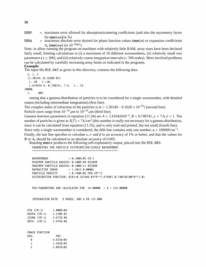
16
ERRP = maximum error allowed for absorption/scattering coefficients (and also the asymmetry factorfor mmmiea)(in %)
ERRA = maximum absolute error desired for phase function values (mmmie) or expansion coefficientsAn (mmmiea) (in 10−digits)
Note: to allow running the program on machines with relatively little RAM, array sizes have been declaredfairly small, limiting calculations to (i) a maximum of 10 different wavenumbers, (ii) relatively small sizeparameters (x . 300), and (iii) relatively coarse integration intervals (< 500 nodes). More involved problemscan be calculated by carefully increasing array limits as indicated in the programs.Example:The input fileMIE.DAT as given in this directory, contains the following data:2, 1, 2
(1.30149,-0.1620E-05)
1.-10 1.+10,
1.619424-4, 0.740741, 7.6, 1., 74.
10000.
1. .005
stating that a gamma-distribution of particles is to be considered for a single wavenumber, with detailedoutput (including intermediate integrations) (first line).The complex index of refraction of the particles ism= 1.30149− 0.1620× 10−05i (second line).Particle sizes range from 10−10µm to 10+10µm (third line).Gamma-function parameters in equation (11.34) areA = 1.61942410−4, B = 0.740741, γ = 7.6, δ = 1. Thenumber of particles is given asN(T) = 74/cm3 (this number is really not necessary for a gamma distribution,since it can be calculated from equation (11.35), and is only read and printed, but not used) (fourth line).Since only a single wavenumber is considered, the fifth line contains only one number,η = 100000 cm−1.Finally, the last line specifies to calculateκ, σ andβ to an accuracy of 1% or better, and that the values forΦ or An should be calculated to an absolute accuracy of 0.005.
Runningmmmie produces the following self-explanatory output, placed into fileMIE.RES:PARAMETERS FOR PARTICLE DISTRIBUTION/SINGLE WAVENUMBER
******************************************************
WAVENUMBER = 0.100E+05 CM-1
MINIMUM PARTICLE RADIUS= 0.100E-09 MICROM
MAXIMUM PARTICLE RADIUS= 0.100E+11 MICROM
REFRACTIVE INDEX = 1.3015-0.0000i
PARTICLE DENSITY = 0.740E+02 PER CM**3
DISTRIBUTION FUNCTION: N(R)=0.16194E-03*R**7.6*EXP(-0.74074E+00*R**1.0)
MIE-PARAMETERS ARE CALCULATED FOR 16.00000 < X < 216.00000
INTEGRATION WITH 9 NODES, AND A DX =25.000
ETA (CM-1) 1.000E+04
KAPPA (CM-1) 1.250E-07
SIGMA (CM-1) 3.675E-04
BETA (CM-1) 3.676E-04
PHASE FUNCTION
DEG. PHI
0 4.835E+03
1 1.943E+03
2 2.093E+02
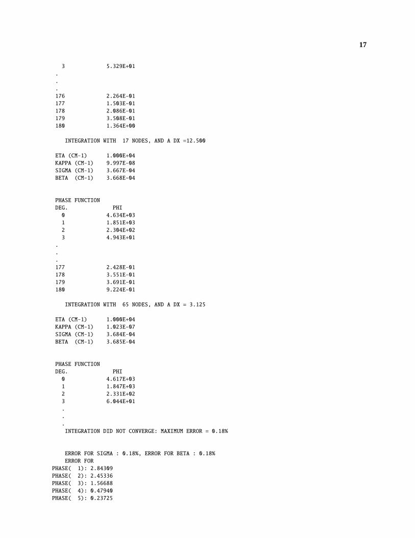
17
3 5.329E+01
.
.
.
176 2.264E-01
177 1.503E-01
178 2.086E-01
179 3.508E-01
180 1.364E+00
INTEGRATION WITH 17 NODES, AND A DX =12.500
ETA (CM-1) 1.000E+04
KAPPA (CM-1) 9.997E-08
SIGMA (CM-1) 3.667E-04
BETA (CM-1) 3.668E-04
PHASE FUNCTION
DEG. PHI
0 4.634E+03
1 1.851E+03
2 2.304E+02
3 4.943E+01
.
.
.
177 2.428E-01
178 3.551E-01
179 3.691E-01
180 9.224E-01
INTEGRATION WITH 65 NODES, AND A DX = 3.125
ETA (CM-1) 1.000E+04
KAPPA (CM-1) 1.023E-07
SIGMA (CM-1) 3.684E-04
BETA (CM-1) 3.685E-04
PHASE FUNCTION
DEG. PHI
0 4.617E+03
1 1.847E+03
2 2.331E+02
3 6.044E+01
.
.
.
INTEGRATION DID NOT CONVERGE: MAXIMUM ERROR = 0.18%
ERROR FOR SIGMA : 0.18%, ERROR FOR BETA : 0.18%
ERROR FOR
PHASE( 1): 2.84309
PHASE( 2): 2.45336
PHASE( 3): 1.56688
PHASE( 4): 0.47940
PHASE( 5): 0.23725

18
.
.
.
PHASE(179): 0.03003
PHASE(180): 0.05414
PHASE(181): 0.10000
ETA (CM-1) 1.000E+04
KAPPA (CM-1) 9.785E-08
SIGMA (CM-1) 3.677E-04
BETA (CM-1) 3.678E-04
PHASE FUNCTION
DEG. PHI
0 4.614E+03
1 1.845E+03
2 2.347E+02
3 6.092E+01
4 3.153E+01
5 2.034E+01
6 1.511E+01
7 1.234E+01
8 1.066E+01
9 9.560E+00
.
.
.
170 7.660E-02
171 1.032E-01
172 1.213E-01
173 1.069E-01
174 9.150E-02
175 1.214E-01
176 1.629E-01
177 2.179E-01
178 2.986E-01
179 2.761E-01
180 7.212E-01
Runningmmmiea, on the other hand produces the following output, placed into fileMIEA.RES:PARAMETERS FOR PARTICLE DISTRIBUTION/SINGLE WAVENUMBER
******************************************************
WAVENUMBER = 0.100E+05 CM-1
MINIMUM PARTICLE RADIUS= 0.100E-09 MICROM
MAXIMUM PARTICLE RADIUS= 0.100E+11 MICROM
REFRACTIVE INDEX = 1.30149-1.62000E-06i
PARTICLE DENSITY = 7.400E+01 PER CM**3
DISTRIBUTION FUNCTION: N(R)=1.61942E-04*R**7.6*EXP(-0.74074E+00*R**1.0)
MIE-PARAMETERS ARE CALCULATED FOR 16.00000 < X < 216.00000
INTEGRATION WITH 9 NODES, AND A DX =25.000

19
ETA (CM-1) 1.000E+04
KAPPA (CM-1) 1.250E-07
SIGMA (CM-1) 3.675E-04
BETA (CM-1) 3.676E-04
GCOS ( -- ) 8.691E-01
A( 1) 2.60744
A( 2) 4.02359
A( 3) 4.85462
A( 4) 5.53582
A( 5) 6.29942
A( 6) 6.88010
A( 7) 7.63828
A( 8) 8.43823
A( 9) 9.15186
.
.
.
A(449) 0.00000
A(450) 0.00000
A(451) 0.00000
A(452) 0.00000
INTEGRATION WITH 33 NODES, AND A DX = 6.250
ETA (CM-1) 1.000E+04
KAPPA (CM-1) 1.015E-07
SIGMA (CM-1) 3.681E-04
BETA (CM-1) 3.682E-04
GCOS ( -- ) 8.716E-01
A( 1) 2.52586
A( 2) 3.88357
A( 3) 4.68158
A( 4) 5.32619
A( 5) 6.04063
A( 6) 6.59512
A( 7) 7.31633
A( 8) 8.08751
A( 9) 8.72379
A( 10) 9.58797
.
.
.
A(449) 0.00000
A(450) 0.00000
A(451) 0.00000
A(452) 0.00000
PHASEFUNCTION
DEG. PHI
0 4.260E+03
5 1.758E+01
10 8.615E+00
15 5.157E+00
20 4.088E+00
25 3.059E+00
30 2.206E+00
35 1.287E+00
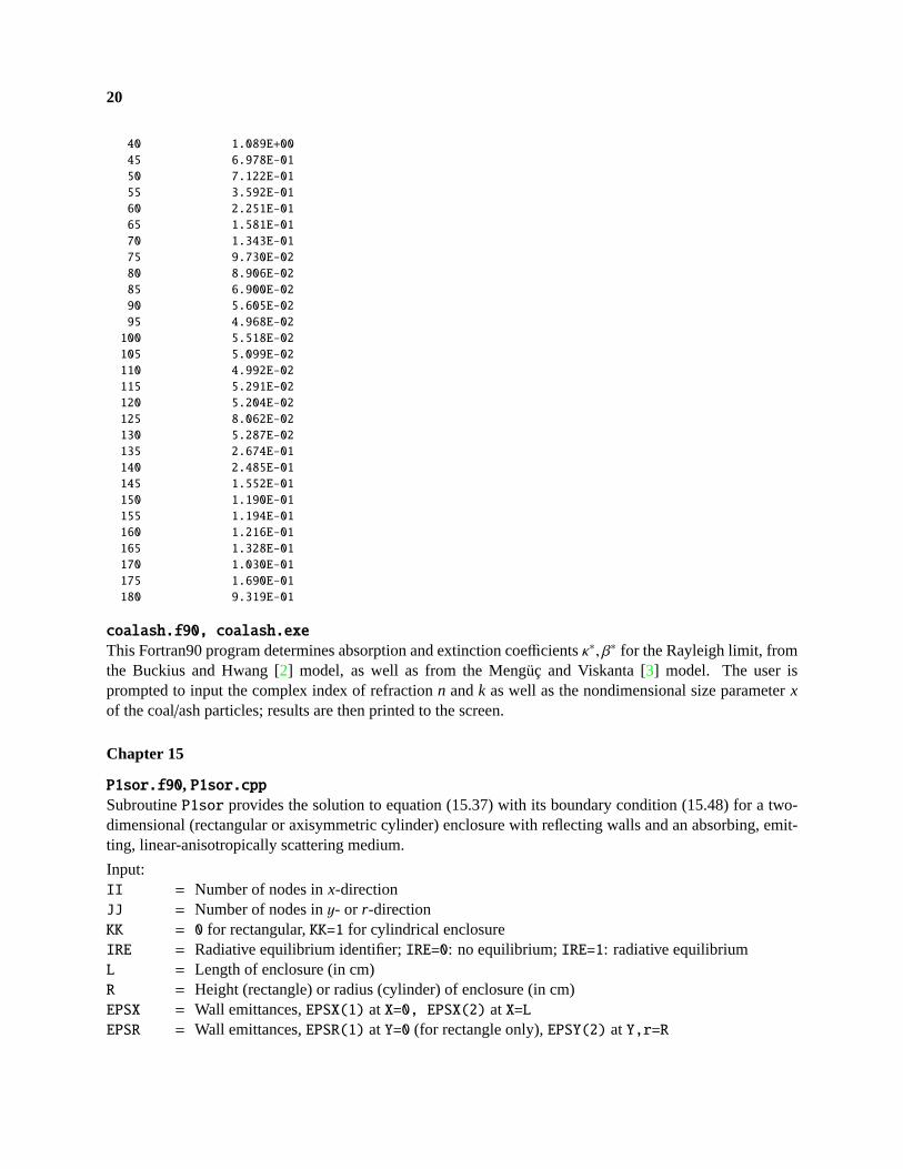
20
40 1.089E+00
45 6.978E-01
50 7.122E-01
55 3.592E-01
60 2.251E-01
65 1.581E-01
70 1.343E-01
75 9.730E-02
80 8.906E-02
85 6.900E-02
90 5.605E-02
95 4.968E-02
100 5.518E-02
105 5.099E-02
110 4.992E-02
115 5.291E-02
120 5.204E-02
125 8.062E-02
130 5.287E-02
135 2.674E-01
140 2.485E-01
145 1.552E-01
150 1.190E-01
155 1.194E-01
160 1.216E-01
165 1.328E-01
170 1.030E-01
175 1.690E-01
180 9.319E-01
coalash.f90, coalash.exe
This Fortran90 program determines absorption and extinction coefficientsκ∗, β∗ for the Rayleigh limit, fromthe Buckius and Hwang [2] model, as well as from the Menguc and Viskanta [3] model. The user isprompted to input the complex index of refractionn andk as well as the nondimensional size parameterxof the coal/ash particles; results are then printed to the screen.
Chapter 15
P1sor.f90, P1sor.cppSubroutineP1sor provides the solution to equation (15.37) with its boundary condition (15.48) for a two-dimensional (rectangular or axisymmetric cylinder) enclosure with reflecting walls and an absorbing, emit-ting, linear-anisotropically scattering medium.
Input:II = Number of nodes inx-directionJJ = Number of nodes iny- or r-directionKK = 0 for rectangular,KK=1 for cylindrical enclosureIRE = Radiative equilibrium identifier;IRE=0: no equilibrium;IRE=1: radiative equilibriumL = Length of enclosure (in cm)R = Height (rectangle) or radius (cylinder) of enclosure (in cm)EPSX = Wall emittances,EPSX(1) atX=0, EPSX(2) atX=LEPSR = Wall emittances,EPSR(1) atY=0 (for rectangle only),EPSY(2) atY,r=R

21
SX = Sources atx-direction walls:SX(1,j=1,2,...JJ) source atx = 0 for varyingy/r-nodesSX(2,j=1,2,...JJ) source atx = L for varyingy/r-nodes(for a standard, gray applicationSX = 4σT4, in W/cm2)
SR = Sources aty, r-direction walls:SR(1,i=1,2,...II) source aty = 0 for varyingx-nodes (for rectangle only)SR(2,i=1,2,...II) source aty, r = R for varyingx-nodes(for a standard, gray applicationSR = 4σT4, in W/cm2)
KT = Absorption coefficient for all internal nodes (in cm−1)ST = Scattering coefficient for all internal nodes (in cm−1)A1 = Linear anisotropy factor for all internal nodesSS = Sources for all internal nodes (in cm−1)
(for a standard, gray applicationSS = 4σT4, in W/cm2)Output:G = Incident radiation for all internal nodes, (in W/cm2)QX = Fluxes atx-direction walls:
QX(1,j=1,2,...JJ) flux at x = 0 for varyingy/r-nodesQX(2,j=1,2,...JJ) flux at x = L for varyingy/R-nodes(positive into positivex-direction, in W/cm2)
QR = Fluxes atx-direction walls:QR(1,i=1,2,...II) flux aty = 0 for varyingx-nodes (for rectangle only)QR(2,i=1,2,...II) flux aty, r = R for varyingx-nodes(positive into positiver, y-direction, in W/cm2)
Calculations can be done for a gray medium or, on a spectral basis, for a nongray medium. For a graymedium the user may either specify a temperature field (IRE=0) by supplyingSS= 4n2σT4, or radiativeequilibrium may be invoked (IRE=1), in which case the heat generation termSS= Q
′′′ must be input. Notethat radiative equilibrium is not possible on a spectral level.
Width L is broken up intoII equally spaced nodes with spacing∆x = L/(II − 1); similarly height/radiusR is broken up intoJJ equally spaced nodes with spacing∆r = R/(JJ − 1).
For each of theII×JJ nodes each of the radiative properties (κ = KT, σs = ST, A1 = A1) must be input,as well as the local radiative sourceSS (= 4πIb if IRE=0, or= Q
′′′ if IRE=1). In addition, for each surfacean emittance must be specified [ε(x = 0) = EPSX(1), ε(x = L) = EPSX(2); ε(y = 0)= EPSR(1) for rectangularenclosures only, andε(rory = R) = EPSR(2)], as well as radiation sources [4πIbw(x = 0) = SX(1), 4πIbw(x =L) = SX(2); 4πIbw(y = 0) = SR(1) for rectangular enclosures only, and 4πIbw(rory = R) = SR(2)]. Insulatedboundaries can be treated by setting the emittance of that surface to zero. One-dimensional problems canbe treated by setting two opposing emittances to zero; for better efficiency the number of nodes in thecross-direction should be set to one. Thus,EPSR(1) = EPSR(2) = 0 andJJ = 1 makes the problem a one-dimensional slab, whileEPSX(1) = EPSX(2) = 0 andII = 1 makes a one-dimensional cylinder.
Upon returnP1sor provides the solution arrayG (incident radiationG for all II×JJ nodes), as well asflux vectorsQX (for radiative fluxes at the two surfacesx = 0 andx = L) andQY (radiative fluxes aty = 0for a rectangle, androry = R). The solution is found bysuccessive over-relaxation, with over-relaxationparameterOM, which is optimized by an implementation of algorithm 9-6.1 given in [4].Code DetailsFor a two-dimensional problem equation (15.37) may be rewritten as
−13
1
rk
∂
∂r
(rk
β∗∂G∂r
)+∂
∂x
(1β∗∂G∂x
)= κ(4πIb −G) temperature specified,
= Q′′′ radiative equilibrium, (CC-8)
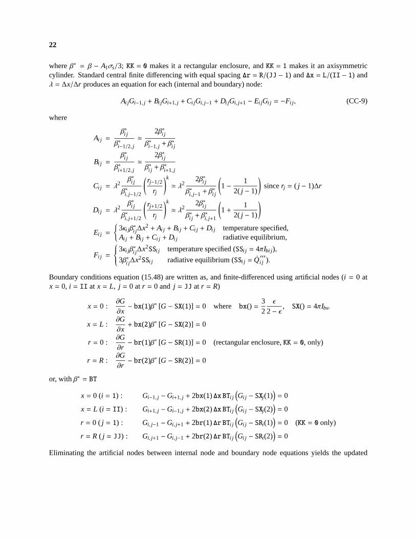
22
whereβ∗ = β − A1σs/3; KK = 0 makes it a rectangular enclosure, andKK = 1 makes it an axisymmetriccylinder. Standard central finite differencing with equal spacing∆r = R/(JJ − 1) and∆x = L/(II − 1) andλ = ∆x/∆r produces an equation for each (internal and boundary) node:
Ai jGi−1, j + Bi jGi+1, j +Ci jGi, j−1 + Di jGi, j+1 − Ei jGi j = −Fi j , (CC-9)
where
Ai j =β∗i j
β∗i−1/2, j
'2β∗i j
β∗i−1, j + β∗i j
Bi j =β∗i j
β∗i+1/2, j
'2β∗i j
β∗i j + β∗i+1, j
Ci j = λ2β∗i j
β∗i, j−1/2
(rj−1/2
rj
)k
' λ22β∗i j
β∗i, j−1 + β∗i j
(1−
12( j − 1)
)sincerj = ( j − 1)∆r
Di j = λ2β∗i j
β∗i, j+1/2
(rj+1/2
rj
)k
' λ22β∗i j
β∗i j + β∗i, j+1
(1+
12( j − 1)
)Ei j =
3κi jβ∗i j∆x2 + Ai j + Bi j +Ci j + Di j temperature specified,Ai j + Bi j +Ci j + Di j radiative equilibrium,
Fi j =
3κi jβ∗i j∆x2SSi j temperature specified (SSi j = 4πIbi j),
3β∗i j∆x2SSi j radiative equilibrium (SSi j = Q′′′
i j ).
Boundary conditions equation (15.48) are written as, and finite-differenced using artificial nodes (i = 0 atx = 0, i = II at x = L, j = 0 atr = 0 and j = JJ at r = R)
x = 0 :∂G∂x− bx(1)β∗ [G − SX(1)] = 0 where bx() =
32ε
2− ε, SX() = 4πIbw
x = L :∂G∂x+ bx(2)β∗ [G − SX(2)] = 0
r = 0 :∂G∂r− br(1)β∗ [G − SR(1)] = 0 (rectangular enclosure,KK = 0, only)
r = R :∂G∂r− br(2)β∗ [G − SR(2)] = 0
or, with β∗ = BT
x = 0 (i = 1) : Gi−1, j −Gi+1, j + 2bx(1) ∆x BTi j(Gi j − SXj(1)
)= 0
x = L (i = II) : Gi+1, j −Gi−1, j + 2bx(2) ∆x BTi j(Gi j − SXj(2)
)= 0
r = 0 ( j = 1) : Gi, j−1 −Gi, j+1 + 2br(1) ∆r BTi j(Gi j − SRi(1)
)= 0 (KK = 0 only)
r = R ( j = JJ) : Gi, j+1 −Gi, j−1 + 2br(2) ∆r BTi j(Gi j − SRi(2)
)= 0
Eliminating the artificial nodes between internal node and boundary node equations yields the updated

23
values
i = 1 : A′i j = 0, B′i j = Ai j + Bi j ,E′i j = Ei j + 2bx(1) ∆x BTi j Ai j
F′i j = Fi j + 2bx(1) ∆x BTi j Ai jSXj(1)
i = II : B′i j = 0,A′i j = Ai j + Bi j ; E′i j = Ei j + 2bx(2) ∆x BTi j Bi j
F′i j = Fi j + 2bx(2) ∆x BTi j Bi jSXj(2)
j = 1 : C′i j = 0,D′i j = Ci j + Di j ,E′i j = Ei j + 2br(1) ∆r BTi jCi j
F′i j = Fi j + 2br(1) ∆r BTi jCi jSRj(1)
j = JJ : D′i j = 0,C′i j = Ci j + Di j ,E′i j = Ei j + 2br(2) ∆r BTi j Di j
F′i j = Fi j + 2br(2) ∆r BTi j Di jSRj(2)
For a cylindrical enclosure (KK = 1) the boundary condition atr = 0 (J = 1) becomes
r = 0, ( j = 1) :∂G∂r= 0 or Gi, j−1 = Gi, j+1.
Also, the governing equation (CC-8) becomes indeterminate. Expanding the radial derivative and using Del’Hopital’s rule, we obtain
limr→0
1r∂
∂r
(rβ∗∂G∂r
)=
1β∗∂2G
∂r2−
1β∗2∂G∂r∂β∗
∂r+ lim
r→0
1rβ∗∂G∂r=
2β∗∂2G
∂r2
=4
βi1∆r2(Gi2 −Gi1)
Thus, forKK = 1 andJ = 1Ci j = 0, Di j = 4λ2
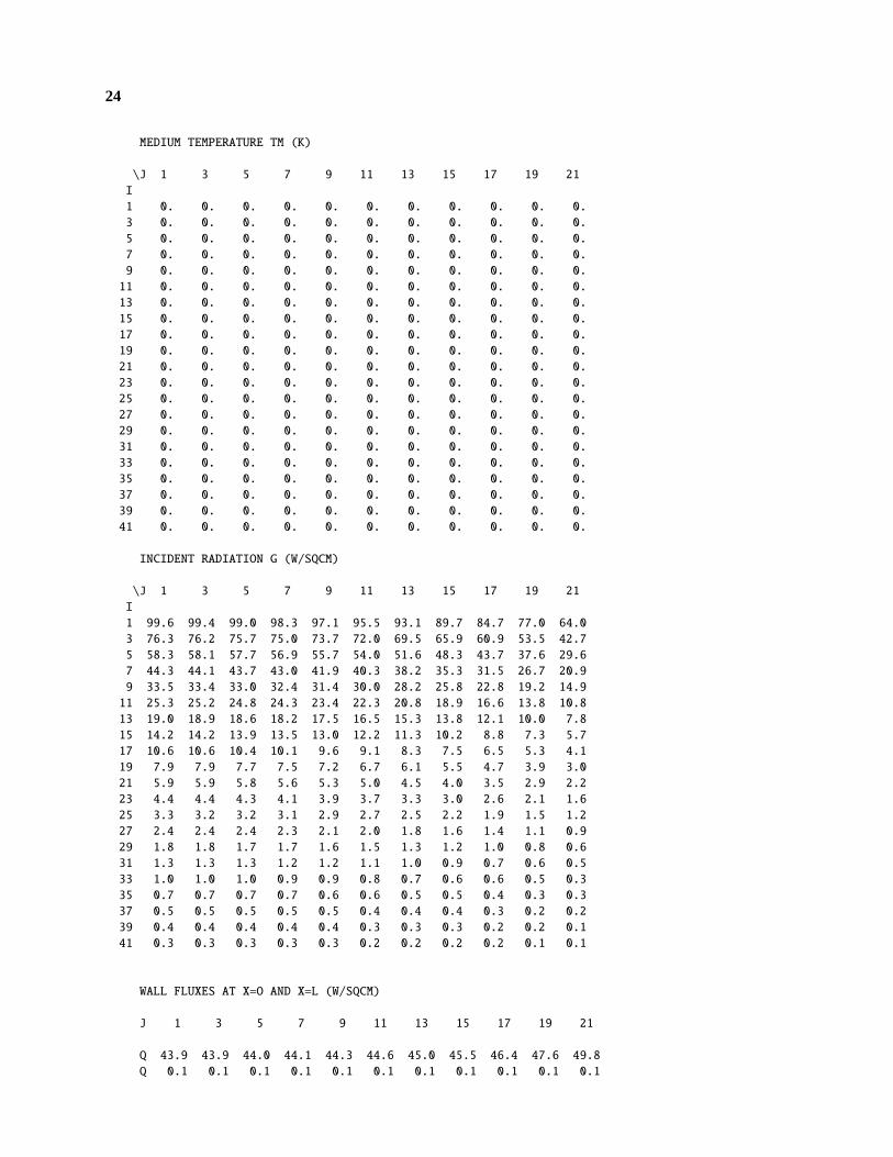
P1-2D.f90, P1-2D.cppProgramP1-2D is a front end for subroutineP1sor, setting up the problem for a gray medium with spatiallyconstant radiative properties (dimensions, radiative properties, and sources from known temperatures); maybe used as a starting point for more involved applications. After callingP1sor the program also generatesappropriate output. As given,P1-2D simulates the case of a two-dimensional axisymmetric cylinder (KK=1)of R = 10 cm radius andL = 20 cm length, usingJJ=21 nodes in the radial direction andII=41 nodesin the axial direction (i.e.,∆x = ∆r = 0.5 cm), with a cold (Ti j = TM = 0) gray medium, with constantabsorption and scattering coefficients (κ = σs = 0.1 cm−1,A1 = 0); bounding walls are black and coldexcept for the face atx = 0, which is gray (EPSX(1)=0.5) and hot (TX(1)=2000K). Since the temperaturefield is specified, we haveIRE=0. RunningP1-2D we find from screen output that the calculation requires97 iterations with a residual 2-norm error of 0.1354× 10⁻⁴.
The output is in fileP1-2Dsor.dat, giving:GENERAL DATA
************
CYLINDER RADIUS (R-DIR): 10.00
CYLINDER LENGTH (X-DIR): 20.00
TEMPERATURE AT r=R(j=J): 0.00K, EMITTANCE 1.00
TEMPERATURE AT x=0(i=1): 2000.00K, EMITTANCE 0.50
TEMPERATURE AT x=L(i=I): 0.00K, EMITTANCE 1.00
24
MEDIUM TEMPERATURE TM (K)
\J 1 3 5 7 9 11 13 15 17 19 21
I
1 0. 0. 0. 0. 0. 0. 0. 0. 0. 0. 0.
3 0. 0. 0. 0. 0. 0. 0. 0. 0. 0. 0.
5 0. 0. 0. 0. 0. 0. 0. 0. 0. 0. 0.
7 0. 0. 0. 0. 0. 0. 0. 0. 0. 0. 0.
9 0. 0. 0. 0. 0. 0. 0. 0. 0. 0. 0.
11 0. 0. 0. 0. 0. 0. 0. 0. 0. 0. 0.
13 0. 0. 0. 0. 0. 0. 0. 0. 0. 0. 0.
15 0. 0. 0. 0. 0. 0. 0. 0. 0. 0. 0.
17 0. 0. 0. 0. 0. 0. 0. 0. 0. 0. 0.
19 0. 0. 0. 0. 0. 0. 0. 0. 0. 0. 0.
21 0. 0. 0. 0. 0. 0. 0. 0. 0. 0. 0.
23 0. 0. 0. 0. 0. 0. 0. 0. 0. 0. 0.
25 0. 0. 0. 0. 0. 0. 0. 0. 0. 0. 0.
27 0. 0. 0. 0. 0. 0. 0. 0. 0. 0. 0.
29 0. 0. 0. 0. 0. 0. 0. 0. 0. 0. 0.
31 0. 0. 0. 0. 0. 0. 0. 0. 0. 0. 0.
33 0. 0. 0. 0. 0. 0. 0. 0. 0. 0. 0.
35 0. 0. 0. 0. 0. 0. 0. 0. 0. 0. 0.
37 0. 0. 0. 0. 0. 0. 0. 0. 0. 0. 0.
39 0. 0. 0. 0. 0. 0. 0. 0. 0. 0. 0.
41 0. 0. 0. 0. 0. 0. 0. 0. 0. 0. 0.
INCIDENT RADIATION G (W/SQCM)
\J 1 3 5 7 9 11 13 15 17 19 21
I
1 99.6 99.4 99.0 98.3 97.1 95.5 93.1 89.7 84.7 77.0 64.0
3 76.3 76.2 75.7 75.0 73.7 72.0 69.5 65.9 60.9 53.5 42.7
5 58.3 58.1 57.7 56.9 55.7 54.0 51.6 48.3 43.7 37.6 29.6
7 44.3 44.1 43.7 43.0 41.9 40.3 38.2 35.3 31.5 26.7 20.9
9 33.5 33.4 33.0 32.4 31.4 30.0 28.2 25.8 22.8 19.2 14.9
11 25.3 25.2 24.8 24.3 23.4 22.3 20.8 18.9 16.6 13.8 10.8
13 19.0 18.9 18.6 18.2 17.5 16.5 15.3 13.8 12.1 10.0 7.8
15 14.2 14.2 13.9 13.5 13.0 12.2 11.3 10.2 8.8 7.3 5.7
17 10.6 10.6 10.4 10.1 9.6 9.1 8.3 7.5 6.5 5.3 4.1
19 7.9 7.9 7.7 7.5 7.2 6.7 6.1 5.5 4.7 3.9 3.0
21 5.9 5.9 5.8 5.6 5.3 5.0 4.5 4.0 3.5 2.9 2.2
23 4.4 4.4 4.3 4.1 3.9 3.7 3.3 3.0 2.6 2.1 1.6
25 3.3 3.2 3.2 3.1 2.9 2.7 2.5 2.2 1.9 1.5 1.2
27 2.4 2.4 2.4 2.3 2.1 2.0 1.8 1.6 1.4 1.1 0.9
29 1.8 1.8 1.7 1.7 1.6 1.5 1.3 1.2 1.0 0.8 0.6
31 1.3 1.3 1.3 1.2 1.2 1.1 1.0 0.9 0.7 0.6 0.5
33 1.0 1.0 1.0 0.9 0.9 0.8 0.7 0.6 0.6 0.5 0.3
35 0.7 0.7 0.7 0.7 0.6 0.6 0.5 0.5 0.4 0.3 0.3
37 0.5 0.5 0.5 0.5 0.5 0.4 0.4 0.4 0.3 0.2 0.2
39 0.4 0.4 0.4 0.4 0.4 0.3 0.3 0.3 0.2 0.2 0.1
41 0.3 0.3 0.3 0.3 0.3 0.2 0.2 0.2 0.2 0.1 0.1
WALL FLUXES AT X=O AND X=L (W/SQCM)
J 1 3 5 7 9 11 13 15 17 19 21
Q 43.9 43.9 44.0 44.1 44.3 44.6 45.0 45.5 46.4 47.6 49.8
Q 0.1 0.1 0.1 0.1 0.1 0.1 0.1 0.1 0.1 0.1 0.1
25
RADIAL FLUXES TO CYLINDER WALL (W/SQCM)
I QR
1 32.0
2 25.9
3 21.3
.
.
.
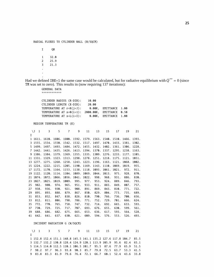
Had we definedIRE=1 the same case would be calculated, but for radiative equilibrium withQ′′′= 0 (since
TM was set to zero). This results in (now requiring 137 iterations):GENERAL DATA
************
CYLINDER RADIUS (R-DIR): 10.00
CYLINDER LENGTH (X-DIR): 20.00
TEMPERATURE AT r=R(j=J): 0.00K, EMITTANCE 1.00
TEMPERATURE AT x=0(i=1): 2000.00K, EMITTANCE 0.50
TEMPERATURE AT x=L(i=I): 0.00K, EMITTANCE 1.00
MEDIUM TEMPERATURE TM (K)
\J 1 3 5 7 9 11 13 15 17 19 21
I
1 1611. 1610. 1606. 1600. 1592. 1579. 1563. 1540. 1510. 1466. 1393.
3 1555. 1554. 1550. 1542. 1532. 1517. 1497. 1470. 1433. 1381. 1302.
5 1499. 1497. 1493. 1484. 1472. 1455. 1432. 1402. 1361. 1306. 1228.
7 1442. 1441. 1435. 1426. 1413. 1394. 1370. 1337. 1295. 1238. 1163.
9 1386. 1384. 1379. 1369. 1355. 1335. 1309. 1276. 1233. 1177. 1105.
11 1331. 1329. 1323. 1313. 1298. 1278. 1251. 1218. 1175. 1121. 1051.
13 1277. 1275. 1268. 1258. 1243. 1223. 1196. 1163. 1121. 1068. 1002.
15 1224. 1222. 1215. 1205. 1190. 1169. 1143. 1110. 1069. 1019. 955.
17 1172. 1170. 1164. 1153. 1138. 1118. 1093. 1061. 1021. 972. 911.
19 1122. 1120. 1114. 1104. 1089. 1069. 1044. 1013. 975. 928. 870.
21 1074. 1072. 1066. 1056. 1041. 1022. 998. 968. 931. 886. 830.
23 1027. 1025. 1019. 1009. 995. 977. 953. 924. 889. 846. 793.
25 982. 980. 974. 965. 951. 933. 911. 883. 849. 807. 757.
27 938. 936. 930. 921. 908. 891. 869. 843. 810. 771. 722.
29 895. 893. 888. 879. 867. 850. 829. 804. 773. 735. 689.
31 853. 852. 847. 838. 826. 810. 790. 766. 736. 700. 656.
33 812. 811. 806. 798. 786. 771. 752. 729. 701. 666. 624.
35 772. 770. 765. 758. 747. 732. 714. 692. 665. 633. 593.
37 730. 729. 725. 717. 707. 693. 676. 655. 630. 599. 561.
39 688. 686. 682. 675. 665. 653. 636. 617. 593. 564. 528.
41 642. 641. 637. 630. 621. 609. 594. 576. 553. 526. 493.
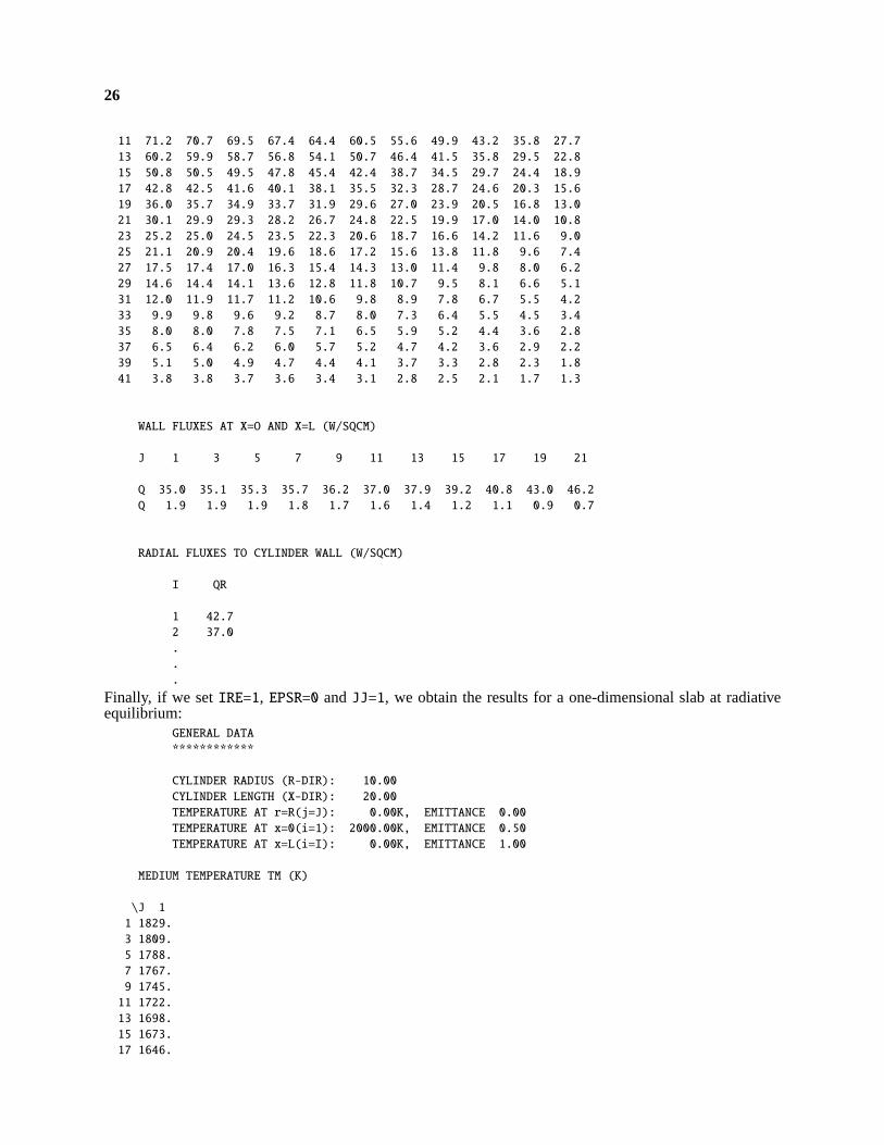
INCIDENT RADIATION G (W/SQCM)
\J 1 3 5 7 9 11 13 15 17 19 21
I
1 152.8 152.4 151.1 148.8 145.5 141.1 135.2 127.6 117.8 104.7 85.5
3 132.7 132.2 130.8 128.4 124.9 120.1 113.9 105.9 95.6 82.4 65.1
5 114.5 114.0 112.5 110.1 106.5 101.7 95.5 87.6 77.9 65.9 51.5
7 98.2 97.7 96.3 93.8 90.3 85.7 79.8 72.5 63.7 53.3 41.5
9 83.8 83.3 81.9 79.6 76.4 72.1 66.7 60.1 52.4 43.6 33.8
26
11 71.2 70.7 69.5 67.4 64.4 60.5 55.6 49.9 43.2 35.8 27.7
13 60.2 59.9 58.7 56.8 54.1 50.7 46.4 41.5 35.8 29.5 22.8
15 50.8 50.5 49.5 47.8 45.4 42.4 38.7 34.5 29.7 24.4 18.9
17 42.8 42.5 41.6 40.1 38.1 35.5 32.3 28.7 24.6 20.3 15.6
19 36.0 35.7 34.9 33.7 31.9 29.6 27.0 23.9 20.5 16.8 13.0
21 30.1 29.9 29.3 28.2 26.7 24.8 22.5 19.9 17.0 14.0 10.8
23 25.2 25.0 24.5 23.5 22.3 20.6 18.7 16.6 14.2 11.6 9.0
25 21.1 20.9 20.4 19.6 18.6 17.2 15.6 13.8 11.8 9.6 7.4
27 17.5 17.4 17.0 16.3 15.4 14.3 13.0 11.4 9.8 8.0 6.2
29 14.6 14.4 14.1 13.6 12.8 11.8 10.7 9.5 8.1 6.6 5.1
31 12.0 11.9 11.7 11.2 10.6 9.8 8.9 7.8 6.7 5.5 4.2
33 9.9 9.8 9.6 9.2 8.7 8.0 7.3 6.4 5.5 4.5 3.4
35 8.0 8.0 7.8 7.5 7.1 6.5 5.9 5.2 4.4 3.6 2.8
37 6.5 6.4 6.2 6.0 5.7 5.2 4.7 4.2 3.6 2.9 2.2
39 5.1 5.0 4.9 4.7 4.4 4.1 3.7 3.3 2.8 2.3 1.8
41 3.8 3.8 3.7 3.6 3.4 3.1 2.8 2.5 2.1 1.7 1.3
WALL FLUXES AT X=O AND X=L (W/SQCM)
J 1 3 5 7 9 11 13 15 17 19 21
Q 35.0 35.1 35.3 35.7 36.2 37.0 37.9 39.2 40.8 43.0 46.2
Q 1.9 1.9 1.9 1.8 1.7 1.6 1.4 1.2 1.1 0.9 0.7
RADIAL FLUXES TO CYLINDER WALL (W/SQCM)
I QR
1 42.7
2 37.0
.
.
.
Finally, if we setIRE=1, EPSR=0 andJJ=1, we obtain the results for a one-dimensional slab at radiativeequilibrium:
GENERAL DATA
************
CYLINDER RADIUS (R-DIR): 10.00
CYLINDER LENGTH (X-DIR): 20.00
TEMPERATURE AT r=R(j=J): 0.00K, EMITTANCE 0.00
TEMPERATURE AT x=0(i=1): 2000.00K, EMITTANCE 0.50
TEMPERATURE AT x=L(i=I): 0.00K, EMITTANCE 1.00
MEDIUM TEMPERATURE TM (K)
\J 1
1 1829.
3 1809.
5 1788.
7 1767.
9 1745.
11 1722.
13 1698.
15 1673.
17 1646.

27
19 1619.
21 1590.
23 1559.
25 1527.
27 1492.
29 1454.
31 1414.
33 1369.
35 1320.
37 1264.
39 1201.
41 1124.
INCIDENT RADIATION G (W/SQCM)
\J 1
1 253.7
3 242.8
5 232.0
7 221.1
9 210.2
11 199.3
13 188.4
15 177.5
17 166.7
19 155.8
21 144.9
23 134.1
25 123.2
27 112.3
29 101.5
31 90.6
33 79.7
35 68.9
37 58.0
39 47.1
41 36.2
WALL FLUXES AT X=O AND X=L (W/SQCM)
J 1
Q 18.2
Q 18.1
RADIAL FLUXES TO CYLINDER WALL (W/SQCM)
I QR
1 0.0
2 0.0
.
.
.
Of course, the matrix for this case could have easily been inverted by a tridiagonal matrix solver (instead ofusing 181 iterations as done here), or could have been found analytically using Example 14.5 (but for a graywall) .
28
Chapter 18
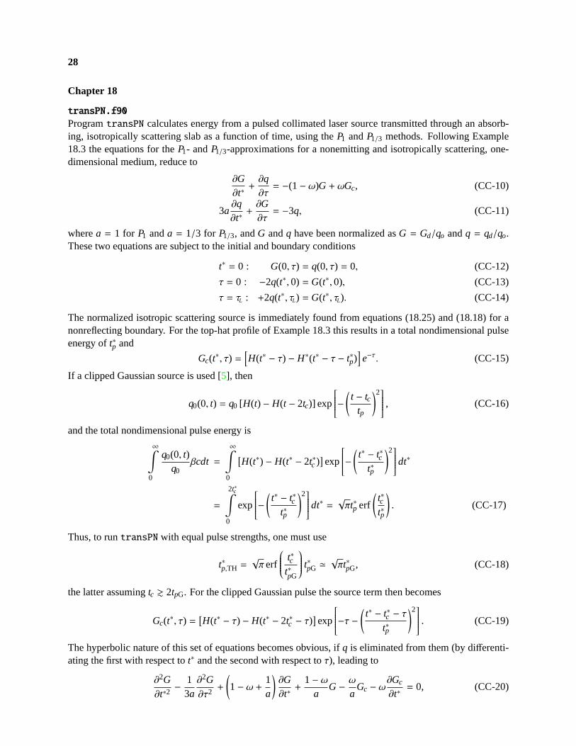
transPN.f90
ProgramtransPN calculates energy from a pulsed collimated laser source transmitted through an absorb-ing, isotropically scattering slab as a function of time, using theP1 andP1/3 methods. Following Example18.3 the equations for theP1- andP1/3-approximations for a nonemitting and isotropically scattering, one-dimensional medium, reduce to
∂G∂t∗+∂q∂τ= −(1− ω)G + ωGc, (CC-10)
3a∂q∂t∗+∂G∂τ= −3q, (CC-11)
wherea = 1 for P1 anda = 1/3 for P1/3, andG andq have been normalized asG = Gd/qo andq = qd/qo.These two equations are subject to the initial and boundary conditions
t∗ = 0 : G(0, τ) = q(0, τ) = 0, (CC-12)
τ = 0 : −2q(t∗,0) = G(t∗,0), (CC-13)
τ = τL : +2q(t∗, τL) = G(t∗, τL). (CC-14)
The normalized isotropic scattering source is immediately found from equations (18.25) and (18.18) for anonreflecting boundary. For the top-hat profile of Example 18.3 this results in a total nondimensional pulseenergy oft∗p and
Gc(t∗, τ) =
[H(t∗ − τ) − H∗(t∗ − τ − t∗p)
]e−τ. (CC-15)
If a clipped Gaussian source is used [5], then
q0(0, t) = q0 [H(t) − H(t − 2tc)] exp
− (t − tc
tp
)2 , (CC-16)
and the total nondimensional pulse energy is
∞∫0
q0(0, t)q0βcdt =
∞∫0
[H(t∗) − H(t∗ − 2t∗c )
]exp
− (t∗ − t∗c
t∗p
)2 dt∗
=
2t∗c∫0
exp
− (t∗ − t∗c
t∗p
)2 dt∗ =√πt∗p erf
(t∗ct∗p
). (CC-17)
Thus, to runtransPN with equal pulse strengths, one must use
t∗p,TH =√πerf
t∗ct∗pG
t∗pG '√πt∗pG, (CC-18)
the latter assumingtc & 2tpG. For the clipped Gaussian pulse the source term then becomes
Gc(t∗, τ) =
[H(t∗ − τ) − H(t∗ − 2t∗c − τ)
]exp
−τ − (t∗ − t∗c − τ
t∗p
)2 . (CC-19)
The hyperbolic nature of this set of equations becomes obvious, ifq is eliminated from them (by differenti-ating the first with respect tot∗ and the second with respect toτ), leading to
∂2G
∂t∗2−
13a∂2G
∂τ2+
(1− ω +
1a
)∂G∂t∗+
1− ωa
G −ω
aGc − ω
∂Gc
∂t∗= 0, (CC-20)

29
1 2 3 i i + 1 Nx0
∆
L
τ
τ
∆t*
t* = - t* =
+
i + ½
n=01
2
3
FIGURE 1Time-space nodal system fortransPN.f90.
which has a signal velocity ofα = 1/√
3a (nondimensional in terms of speed of light,c), as already indicatedin the formulation for thePa methods. Eliminatingq also from initial and boundary conditions gives
t∗ = 0 : G(0, τ) =∂G∂t∗
(0, τ) = 0, (CC-21)
τ = 0 : 3
(G(t∗,0)+ a
∂G∂t∗
(t∗,0)
)− 2∂G∂τ
(t∗,0) = 0, (CC-22)
τ = τL : 3
(G(t∗,0)+ a
∂G∂t∗
(t∗,0)
)+ 2∂G∂τ
(t∗,0) = 0. (CC-23)
This second-order hyperbolic equation is readily solved by the method of characteristics [6] along the char-acteristic linesτ = ±αt∗. Using subscript notation, i.e.,Gx = ∂G/∂τ, etc., equation (CC-20) may berewritten as
Gtt − α2Gxx+ (1− ω)Gt + 3α2
[Gt + (1− ω)G − ωG
′
c
]= 0, (CC-24)
whereG′
c = Gc + ∂Gc/∂t∗. Along the two characteristic linesτ = ±αt∗ we have [6]
±αdGt − α2dGx ±
(1− ω)Gt + 3α2
[Gt + (1− ω)G − ωG
′
c
]dτ = 0 (CC-25)
and the total differential isdG= Gtdt∗ +Gxdτ. (CC-26)
We will break up the thickness of the slab,L, into Nx equally-spaced nodes of width∆x = L/Nx, or∆τ = τL/Nx. In t∗-τ-space the characteristics then are straight lines as shown in Fig. 1Chapter 18figure.0.1,with the lines going up to the right corresponding to the upper sign in equation (CC-25), and the linesgoing down to the right to the lower sign. As time step∆τ we take the time it takes to move along thecharacteristics from adjacent points (n, i) and (n, i + 1) to their intersection at (n+ 1, i + 1/2) as shown in thefigure. During that time the signal moves a distance±∆x/2, so that
∆t∗ = ∆τ/2α. (CC-27)
We can finite-difference equations (CC-25) and (CC-26) along the characteristics by usingdφ = φni+1/2−φn−1
i
for the left-to-right characteristics, anddφ = φni+1/2− φn−1
i+1 for the right-to-left characteristics, whereφ standsfor any of the variablesτ, G, Gt andGx. In the finite differencing we distinguish between odd time steps(all nodes, such asi + 1/2, are internal) and even time steps (all nodes are at integer locations, including twoboundary nodesi = 0 andi = Nx).
30
Odd Time Steps (n odd) All new positions are ati + 1/2 (i = 0,1...Nx − 1); all old positions are ati(i = 0,Nx−1) for the left-to-right characteristics, and ati+1 (i+1 = 1,Nx) for the right-to-left characteristics.Thus,
α(Gt,i+1/2 −Gt,i) − α2(Gx,i+1/2 −Gx,i) +
(1− ω)(Gt,i+1/2 +Gt,i)
+ 3α2[Gt,i+1/2 +Gt,i + (1− ω)(Gi+1/2 +Gi) − ω(G
′
c,i+1/2+G
′
c,i)] ∆τ
4= 0, (CC-28)
where we have used averaged values,φ = 12(φn
i+1/2+ φn−1
i ) for the terms within braces, and have omitted thetime superscripts, since the distinction between new and old is clear. Bringing all unknown quantities at thenew time to the left-hand side we get
BpGt,i+1/2 −C4Gx,i+1/2 +C2Gi+1/2 = −BmGt,i −C4Gx,i −C2Gi +C3(G′
c,i+1/2+G
′
c,i) = E1,
i = 0,Nx − 1, (CC-29)
where
Bp = α + (1− ω + 3α2)∆τ
4, Bm = α − (1− ω + 3α2)
∆τ
4,
C2 = 3α2(1− ω)∆τ
4, C3 = 3α2ω
∆τ
4, C4 = α
2. (CC-30)
Similarly, we obtain for the right-to-left characteristics, by switching the signs in equation (CC-25) andreplacingi by i + 1:
BpGt,i+1/2 +C4Gx,i+1/2 +C2Gi+1/2
= −BmGt,i+1 +C4Gx,i+1 −C2Gi+1 +C3(G′
c,i+1/2+G
′
c,i+1) = E2, i = 0,Nx − 1. (CC-31)
We now have two equations in the three unknownsGt,i+1/2, Gx,i+1/2 andGi+1/2: one more relation is needed andwill come from equation (CC-26), which may be finite-differenced from the left or from the right as
Gi+1/2 = Gi +12
(Gt,i+1/2 +Gt,i)∆t∗ +12
(Gx,i+1/2 +Gx,i)∆τ
2, l → r
= Gi+1 +12
(Gt,i+1/2 +Gt,i+1)∆t∗ −12
(Gx,i+1/2 +Gx,i+1)∆τ
2, r → l. (CC-32)
For better accuracy, we take the average, or
−∆t∗
2Gt,i+1/2 +Gi+1/2 =
12
(Gi +Gi+1) +∆t∗
4(Gt,i +Gt,i+1) +
∆τ
8(Gx,i −Gx,i+1) = D2. (CC-33)
Subtracting equation (CC-29) from (CC-31) leads to
Gx,i+1/2 = (E2 − E1)/2C4, i = 0,Nx − 1, (CC-34)
while adding them gives
BpGt,i+1/2 +C2Gi+1/2 =12
(E1 + E2) = D1, (CC-35)
which, together with equation (CC-33) leads to
Gi+1/2 =D1∆t∗/2+ D2Bp
C2∆t∗/2+ Bp, Gt,i+1/2 =
D1 −C2D2
C2∆t∗/2+ Bp, i = 0,Nx − 1.
31
Even Time Steps (n even) Even time steps are a little more difficult to handle, because two of the nodeslie on the boundaries, and for them the boundary conditions must be invoked. Internal nodes, on the otherhand, are the same as those for oddn, except that nodes are displaced by half a node. Replacing everyi byi − 1/2 we obtain
Gx,i = (E2 − E1)/2C4, Gt,i =D1 −C2D2
C2∆t∗/2+ Bp,
Gi =D1∆t∗/2+ D2Bp
C2∆t∗/2+ Bp; i = 1,Nx − 1, (CC-36)
where
E1 = −BmGt,i−1/2 −C4Gx,i−1/2 −C2Gi− 12+C3(G
′
c,i +G′
c,i−1/2)
E2 = −BmGt,i+1/2 +C4Gx,i+1/2 −C2Gi+ 12+C3(G
′
c,i +G′
c,i+1/2)
D1 =12
(E1 + E2)
D2 = (Gi−1/2 +Gi+1/2) +∆t∗
4(Gt,i−1/2 +Gt,i+1/2) +
∆τ
8(Gx,i−1/2 −Gx,i+1/2)
At the left boundary,i = 0, equation (CC-29) is not valid and must be replaced by the boundary condition,slightly rewritten as
Gx,i =32
Gi +1
2α2Gt,i . (CC-37)
Sticking this into equation (CC-31) (with i + 1/2 replaced byi) gives
f1Gt,i + f2Gi = E2; f1 = Bp +C4
2α2= Bp +
12
; f2 = C2 +32
C4. (CC-38)
Also, for the total derivative we can only use ther → l form, or
Gi = Gi+1/2 +12
(Gt,i +Gt,i+1/2)∆t∗ −12
(Gx,i +Gx,i+1/2)∆τ
2, (CC-39)
or, after eliminatingGx,i through equation (CC-37)
f3Gt,i + f4Gi = D2, f3 =∆τ
8α2−∆t∗
2; f4 = 1+
3∆τ8
, (CC-40)
and, thus,
Gi =f3E2 − f1D2
f3 f2 − f1 f4; Gt,i =
f2D2 − f4E2
f3 f2 − f1 f4, (CC-41)
andGx,i from equation (CC-37).Similarly, for i = Nx equation (CC-31) is not valid and must be replaced by the boundary atτ = τL, and
for the total derivative thel → r version must be used, leading to very similar expressions.Finally, transmissivity and reflectivity of the slab are simply the absolute value of the nondimensional
fluxes at the boundaries, i.e.,
Reflectivity =∣∣∣q(t∗,0
∣∣∣ = 12
G(t∗,0)
Transmissivity = q(t∗, τL) + qc(t∗, τL) =
12
G(t∗, τL) +Gc(t∗, τL). (CC-42)
32
Input:Nx = Number of equally-spaced nodes across slab,a = Pa-approximation switch:a = 1 for P1-approximation,a = 1/3 for P1/3-approximation,L = Thickness of slab, in m,beta = Extinction coefficientβ, in m−1,omga = single scattering albedo,ω,tmax = Maximum t∗max to be considered in calculation,tps = Total nondimensional pulse energy,tme = Starting time for calculation;tme = 0 will start top-hat pulse att∗ = 0, tme = −tps/2 will
center top-hat pulse att∗ = 0, etc.tc,tp = Pulse parameters for clipped-Gaussian pulse; note thattp = tps/
√π results in a total pulse
energy oftps (i.e., the same as for the top-hat pulse).Output:
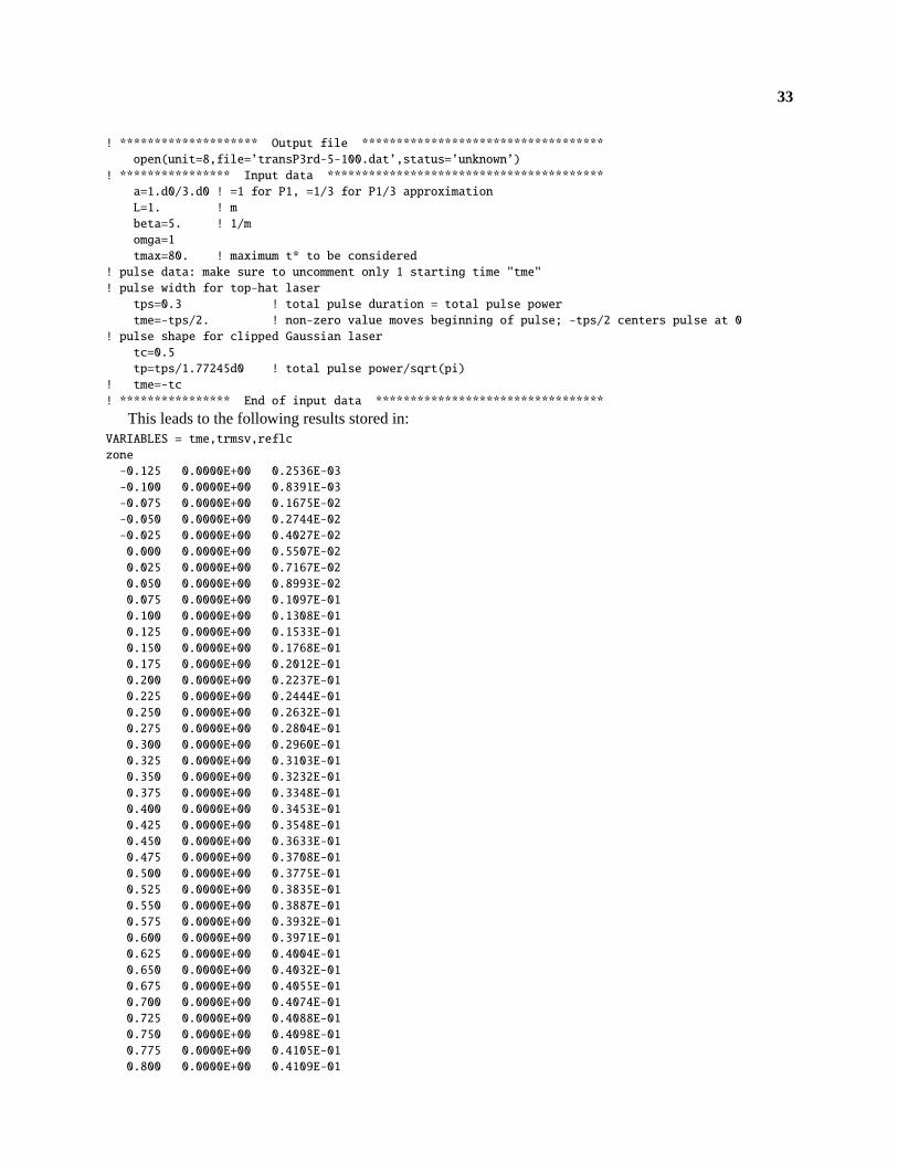
For every even time step the program prints out the value fortme = t∗, Transmissivity and Reflectivity asdefined in equation (CC-42). Total pulse energy, total time integrated reflectivity and transmissivity arealso printed out, which — forω = 1 — gives a check of truncation error and the proper choice fortmax tosimulate the entire pulse.
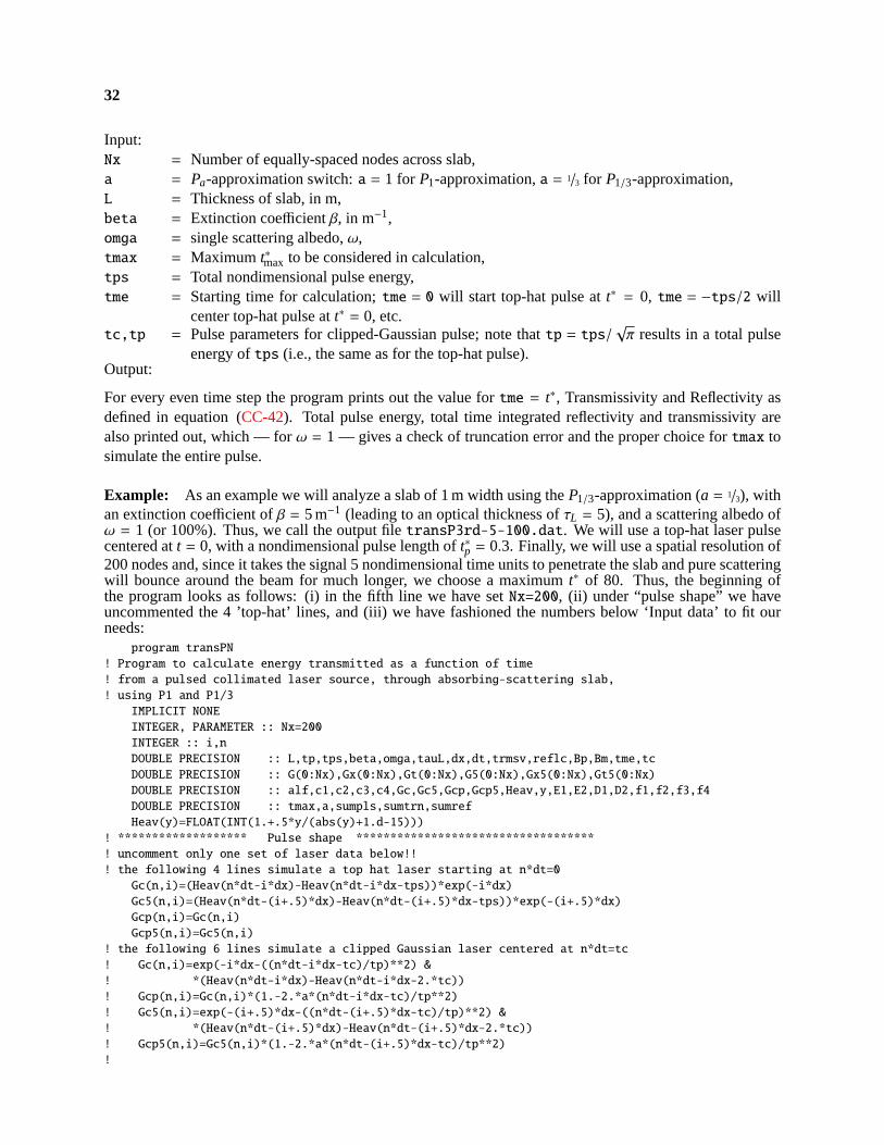
Example: As an example we will analyze a slab of 1 m width using theP1/3-approximation (a = 1/3), withan extinction coefficient ofβ = 5 m−1 (leading to an optical thickness ofτL = 5), and a scattering albedo ofω = 1 (or 100%). Thus, we call the output filetransP3rd-5-100.dat. We will use a top-hat laser pulsecentered att = 0, with a nondimensional pulse length oft∗p = 0.3. Finally, we will use a spatial resolution of200 nodes and, since it takes the signal 5 nondimensional time units to penetrate the slab and pure scatteringwill bounce around the beam for much longer, we choose a maximumt∗ of 80. Thus, the beginning ofthe program looks as follows: (i) in the fifth line we have setNx=200, (ii) under “pulse shape” we haveuncommented the 4 ’top-hat’ lines, and (iii) we have fashioned the numbers below ‘Input data’ to fit ourneeds:
program transPN
! Program to calculate energy transmitted as a function of time
! from a pulsed collimated laser source, through absorbing-scattering slab,
! using P1 and P1/3
IMPLICIT NONE
INTEGER, PARAMETER :: Nx=200
INTEGER :: i,n
DOUBLE PRECISION :: L,tp,tps,beta,omga,tauL,dx,dt,trmsv,reflc,Bp,Bm,tme,tc
DOUBLE PRECISION :: G(0:Nx),Gx(0:Nx),Gt(0:Nx),G5(0:Nx),Gx5(0:Nx),Gt5(0:Nx)
DOUBLE PRECISION :: alf,c1,c2,c3,c4,Gc,Gc5,Gcp,Gcp5,Heav,y,E1,E2,D1,D2,f1,f2,f3,f4
DOUBLE PRECISION :: tmax,a,sumpls,sumtrn,sumref
Heav(y)=FLOAT(INT(1.+.5*y/(abs(y)+1.d-15)))
! ******************* Pulse shape ***********************************
! uncomment only one set of laser data below!!
! the following 4 lines simulate a top hat laser starting at n*dt=0
Gc(n,i)=(Heav(n*dt-i*dx)-Heav(n*dt-i*dx-tps))*exp(-i*dx)
Gc5(n,i)=(Heav(n*dt-(i+.5)*dx)-Heav(n*dt-(i+.5)*dx-tps))*exp(-(i+.5)*dx)
Gcp(n,i)=Gc(n,i)
Gcp5(n,i)=Gc5(n,i)
! the following 6 lines simulate a clipped Gaussian laser centered at n*dt=tc
! Gc(n,i)=exp(-i*dx-((n*dt-i*dx-tc)/tp)**2) &
! *(Heav(n*dt-i*dx)-Heav(n*dt-i*dx-2.*tc))
! Gcp(n,i)=Gc(n,i)*(1.-2.*a*(n*dt-i*dx-tc)/tp**2)
! Gc5(n,i)=exp(-(i+.5)*dx-((n*dt-(i+.5)*dx-tc)/tp)**2) &
! *(Heav(n*dt-(i+.5)*dx)-Heav(n*dt-(i+.5)*dx-2.*tc))
! Gcp5(n,i)=Gc5(n,i)*(1.-2.*a*(n*dt-(i+.5)*dx-tc)/tp**2)
!
33
! ******************** Output file ***********************************
open(unit=8,file=’transP3rd-5-100.dat’,status=’unknown’)
! **************** Input data ****************************************
a=1.d0/3.d0 ! =1 for P1, =1/3 for P1/3 approximation
L=1. ! m
beta=5. ! 1/m
omga=1
tmax=80. ! maximum t* to be considered
! pulse data: make sure to uncomment only 1 starting time "tme"
! pulse width for top-hat laser
tps=0.3 ! total pulse duration = total pulse power
tme=-tps/2. ! non-zero value moves beginning of pulse; -tps/2 centers pulse at 0
! pulse shape for clipped Gaussian laser
tc=0.5
tp=tps/1.77245d0 ! total pulse power/sqrt(pi)
! tme=-tc
! **************** End of input data *********************************
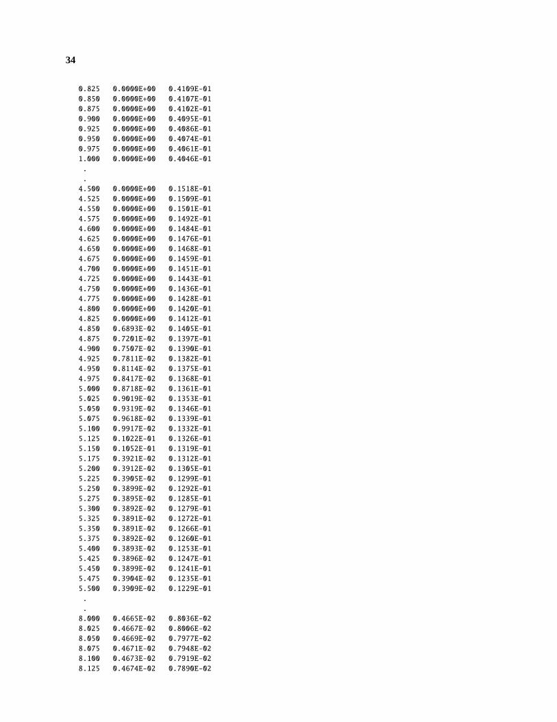
This leads to the following results stored in:VARIABLES = tme,trmsv,reflc
zone
-0.125 0.0000E+00 0.2536E-03
-0.100 0.0000E+00 0.8391E-03
-0.075 0.0000E+00 0.1675E-02
-0.050 0.0000E+00 0.2744E-02
-0.025 0.0000E+00 0.4027E-02
0.000 0.0000E+00 0.5507E-02
0.025 0.0000E+00 0.7167E-02
0.050 0.0000E+00 0.8993E-02
0.075 0.0000E+00 0.1097E-01
0.100 0.0000E+00 0.1308E-01
0.125 0.0000E+00 0.1533E-01
0.150 0.0000E+00 0.1768E-01
0.175 0.0000E+00 0.2012E-01
0.200 0.0000E+00 0.2237E-01
0.225 0.0000E+00 0.2444E-01
0.250 0.0000E+00 0.2632E-01
0.275 0.0000E+00 0.2804E-01
0.300 0.0000E+00 0.2960E-01
0.325 0.0000E+00 0.3103E-01
0.350 0.0000E+00 0.3232E-01
0.375 0.0000E+00 0.3348E-01
0.400 0.0000E+00 0.3453E-01
0.425 0.0000E+00 0.3548E-01
0.450 0.0000E+00 0.3633E-01
0.475 0.0000E+00 0.3708E-01
0.500 0.0000E+00 0.3775E-01
0.525 0.0000E+00 0.3835E-01
0.550 0.0000E+00 0.3887E-01
0.575 0.0000E+00 0.3932E-01
0.600 0.0000E+00 0.3971E-01
0.625 0.0000E+00 0.4004E-01
0.650 0.0000E+00 0.4032E-01
0.675 0.0000E+00 0.4055E-01
0.700 0.0000E+00 0.4074E-01
0.725 0.0000E+00 0.4088E-01
0.750 0.0000E+00 0.4098E-01
0.775 0.0000E+00 0.4105E-01
0.800 0.0000E+00 0.4109E-01
34
0.825 0.0000E+00 0.4109E-01
0.850 0.0000E+00 0.4107E-01
0.875 0.0000E+00 0.4102E-01
0.900 0.0000E+00 0.4095E-01
0.925 0.0000E+00 0.4086E-01
0.950 0.0000E+00 0.4074E-01
0.975 0.0000E+00 0.4061E-01
1.000 0.0000E+00 0.4046E-01
.
.
4.500 0.0000E+00 0.1518E-01
4.525 0.0000E+00 0.1509E-01
4.550 0.0000E+00 0.1501E-01
4.575 0.0000E+00 0.1492E-01
4.600 0.0000E+00 0.1484E-01
4.625 0.0000E+00 0.1476E-01
4.650 0.0000E+00 0.1468E-01
4.675 0.0000E+00 0.1459E-01
4.700 0.0000E+00 0.1451E-01
4.725 0.0000E+00 0.1443E-01
4.750 0.0000E+00 0.1436E-01
4.775 0.0000E+00 0.1428E-01
4.800 0.0000E+00 0.1420E-01
4.825 0.0000E+00 0.1412E-01
4.850 0.6893E-02 0.1405E-01
4.875 0.7201E-02 0.1397E-01
4.900 0.7507E-02 0.1390E-01
4.925 0.7811E-02 0.1382E-01
4.950 0.8114E-02 0.1375E-01
4.975 0.8417E-02 0.1368E-01
5.000 0.8718E-02 0.1361E-01
5.025 0.9019E-02 0.1353E-01
5.050 0.9319E-02 0.1346E-01
5.075 0.9618E-02 0.1339E-01
5.100 0.9917E-02 0.1332E-01
5.125 0.1022E-01 0.1326E-01
5.150 0.1052E-01 0.1319E-01
5.175 0.3921E-02 0.1312E-01
5.200 0.3912E-02 0.1305E-01
5.225 0.3905E-02 0.1299E-01
5.250 0.3899E-02 0.1292E-01
5.275 0.3895E-02 0.1285E-01
5.300 0.3892E-02 0.1279E-01
5.325 0.3891E-02 0.1272E-01
5.350 0.3891E-02 0.1266E-01
5.375 0.3892E-02 0.1260E-01
5.400 0.3893E-02 0.1253E-01
5.425 0.3896E-02 0.1247E-01
5.450 0.3899E-02 0.1241E-01
5.475 0.3904E-02 0.1235E-01
5.500 0.3909E-02 0.1229E-01
.
.
8.000 0.4665E-02 0.8036E-02
8.025 0.4667E-02 0.8006E-02
8.050 0.4669E-02 0.7977E-02
8.075 0.4671E-02 0.7948E-02
8.100 0.4673E-02 0.7919E-02
8.125 0.4674E-02 0.7890E-02

35
8.150 0.4676E-02 0.7861E-02
8.175 0.4677E-02 0.7833E-02
8.200 0.4679E-02 0.7804E-02
8.225 0.4680E-02 0.7776E-02
8.250 0.4681E-02 0.7748E-02
8.275 0.4682E-02 0.7720E-02
8.300 0.4683E-02 0.7693E-02
8.325 0.4684E-02 0.7665E-02
8.350 0.4685E-02 0.7638E-02
8.375 0.4685E-02 0.7611E-02
8.400 0.4686E-02 0.7584E-02
8.425 0.4686E-02 0.7557E-02
8.450 0.4687E-02 0.7530E-02
8.475 0.4687E-02 0.7504E-02
8.500 0.4687E-02 0.7477E-02
8.525 0.4687E-02 0.7451E-02
8.550 0.4687E-02 0.7425E-02
8.575 0.4687E-02 0.7399E-02
8.600 0.4687E-02 0.7373E-02
8.625 0.4687E-02 0.7348E-02
8.650 0.4686E-02 0.7322E-02
8.675 0.4686E-02 0.7297E-02
8.700 0.4685E-02 0.7272E-02
8.725 0.4685E-02 0.7247E-02
8.750 0.4684E-02 0.7222E-02
8.775 0.4683E-02 0.7197E-02
8.800 0.4682E-02 0.7173E-02
8.825 0.4681E-02 0.7148E-02
8.850 0.4680E-02 0.7124E-02
8.875 0.4679E-02 0.7100E-02
8.900 0.4678E-02 0.7076E-02
8.925 0.4677E-02 0.7052E-02
8.950 0.4675E-02 0.7028E-02
8.975 0.4674E-02 0.7004E-02
9.000 0.4673E-02 0.6981E-02
.
.
79.900 0.1443E-04 0.1431E-04
79.925 0.1440E-04 0.1428E-04
79.950 0.1437E-04 0.1425E-04
79.975 0.1434E-04 0.1422E-04
80.000 0.1431E-04 0.1419E-04
80.025 0.1428E-04 0.1416E-04
Total transmission: 8.525E-02
Total reflection: 2.394E-01
Total trans+reflec: 3.246E-01
Total pulse enrg: 3.063E-01
Note that the transmissivity remains 0 untilt∗ = 4.85, when the beginning of the pulse has reached theopposite end by direct travel, and has its maximum at aroundt∗ ' 8.6 (while the reflectivity peaks aroundt∗ ' 0.8. Note that, for the present case of conservative scatteringω = 1, the sum of transmissivity andreflectivity should equal the total pulse energy, or 0.3 (= t∗p). The departures are due to the relatively coarsegrid and the nonconservative nature of thePa-approximation.
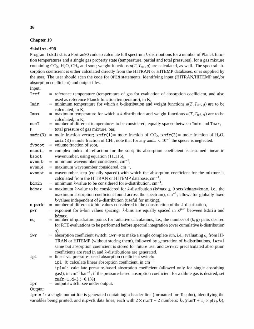
36
Chapter 19
fskdist.f90
Programfskdist is a Fortran90 code to calculate full spectrumk-distributions for a number of Planck func-tion temperatures and a single gas property state (temperature, partial and total pressures), for a gas mixturecontaining CO2, H2O, CH4 and soot; weight functionsa(T,Tref, g) are calculated, as well. The spectral ab-sorption coefficient is either calculated directly from the HITRAN or HITEMP databases, or is supplied bythe user. The user should scan the code forOPEN statements, identifying input (HITRAN/HITEMP and/orabsorption coefficient) and output files.Input:Tref = reference temperature (temperature of gas for evaluation of absorption coefficient, and also
used as reference Planck function temperature), in K,Tmin = minimum temperature for which ak-distribution and weight functionsa(T,Tref, g) are to be
calculated, in K,Tmax = maximum temperature for which ak-distribution and weight functionsa(T,Tref, g) are to be
calculated, in K,numT = number of different temperatures to be considered; equally spaced betweenTmin andTmax,P = total pressure of gas mixture, bar,xmfr(3) = mole fraction vector;xmfr(1)= mole fraction of CO2, xmfr(2)= mole fraction of H2O,
xmfr(3)= mole fraction of CH4; note that for anyxmfr < 10−3 the specie is neglected.fvsoot = volume fraction of soot,nsoot,
ksoot
= complex index of refraction for the soot; its absorption coefficient is assumed linear inwavenumber, using equation (11.116),
wvnm b = minimum wavenumber considered, cm−1,wvnm e = maximum wavenumber considered, cm−1,wvnmst = wavenumber step (equally spaced) with which the absorption coefficient for the mixture is
calculated from the HITRAN or HITEMP database, cm−1,kdmin = minimumk-value to be considered fork-distribution, cm−1,kdmax = maximumk-value to be considered fork-distribution (kdmax ≤ 0 setskdmax=kmax, i.e., the
maximum absorption coefficient found across the spectrum), cm−1; allows for globally fixedk-values independent ofk-distribution (useful for mixing),
n pwrk = number of differentk-bin values considered in the construction of thek-distribution,pwr = exponent fork-bin values spacing:k-bins are equally spaced inkpwr betweenkdmin and
kdmax.nq = number of quadrature points for radiative calculations, i.e., the number of (k, g)-pairs desired
for RTE evaluations to be performed before spectral integration (over cumulativek-distributiong),
iwr = absorption coefficient switch:iwr=0 to make a single complete run, i.e., evaluatingκη from HI-TRAN or HITEMP (without storing them), followed by generation ofk-distributions,iwr=1same but absorption coefficient is stored for future use, andiwr=2: precalculated absorptioncoefficients are read in andk-distributions are generated.
ipl = linear vs. pressure-based absorption coefficient switch:ipl=0: calculate linear absorption coefficient, in cm−1
ipl=1: calculate pressure-based absorption coefficient (allowed only for single absorbinggas!), in cm−1 bar−1; if the pressure-based absorption coefficient for a dilute gas is desired, setxmfr=1.d-3 (=0.1%)
ipr = output switch: see under output.Output:ipr = 1: a single output file is generated containing a header line (formatted for Tecplot), identifying thevariables being printed, andn pwrk data lines, each with 2× numT + 2 numbers:ki , (numT + 1) × g(Tj , ki),

37
and (slightly smoothened)numT × a(Tj ,Tref, ki) (includingTref for g.)ipr = 2: in addition to theipr=1 output file, a second file is generated, containing a header identify-ing variables, andnq output lines, each withnumT+3 numbers:wi , gi(Tref, ki), ki , andnumT smootheneda(Tj ,Tref, ki)-values (averaged over itsg-range).Example:We consider the full-spectrumk-distribution for a pressure-based absorption coefficient (ipl=1) of pureH2O, for a vanishingly small mole fraction (xmfr(3)=(/0.0d0,1.0d-3,0.d0/)). Note thatxH2O hasbeen set to 10−3: the code, when accessing HITRAN or HITEMP, will assume a specie not to be presentwheneverxi < 10−3. The absorption coefficient has been calculated in a previous run (iwr=2), and has beenstored in filec:\absco\absch2o-0p-2000K.dat (for a wavenumber range from 50 cm−1 to 12000 cm−1
with a∆η = 0.01 cm−1). We will calculate thek-distributions for 5 temperatures: a reference temperatureTref = T0 = 2000 K (at which the absorption coefficient has been evaluated) and 4 equally spaced (Planckfunction) temperatures betweenTmin = 0 K andTmax = 1500 K (numT=4): this results in the 4 temperaturesof 300 K, 500 K, 1000 K and 1500 K (the first temperature is not 0 K, because temperatures below 300 Kare not accepted: any temperature below it is set to 300 K). We will use 500k-bins (n_pwrk=500) withpwr=0.1 (this spreads thek-bins over many orders of magnitude, but places more and more bins into largemagnitudes; see output file). We also setkdmin=10−7 (cm−1 bar−1) andkdmax = −20 < 0 (cm−1 bar−1),i.e., we will considerk-values between 10−7 and the maximum value found among the absorption coefficientvalues. Finally, we setipr=2 andnq=12, i.e., besides the generalk-distributions we want to also generatetruncatedk-distributions ready-made for numerical quadrature, using 12 quadrature points. The top of theprogram with input parameters, therefore, looks like this:MODULE Key
IMPLICIT NONE
!HITRAN/HITEMP DATABASE
INTEGER :: lu
INTEGER,PARAMETER :: rows=1400000
DOUBLE PRECISION,PARAMETER :: wvnm_b=50.d0,wvnm_e=12000.d0,wvnmst=0.01d0, &
kdmin=1.d-7,kdmax=-20.d0
DOUBLE PRECISION :: data(rows,6)
END MODULE Key
PROGRAM Main
USE Key
! Input parameters
INTEGER,PARAMETER :: numT=4,n_pwrk=500,iwr=2,ipl=1,ipr=2,nq=12
DOUBLE PRECISION,PARAMETER :: P=1.d0,Tref=2000d0,Tmin=000d0,Tmax=1500d0
DOUBLE PRECISION,PARAMETER :: xmfr(3)=(/0.0d0,1.0d-3,0.d0/)
DOUBLE PRECISION,PARAMETER :: klmin=1.d-9,pwr=0.1d0
DOUBLE PRECISION,PARAMETER :: fvsoot=0.d-6,nsoot=1.89d0,ksoot=0.92d0
where we have changed the values forwvnm_b, wvnm_e, wvnmst, kdmin, kdmax, numT, n_pwrk,iwr, ipl, ipr, nq, Tref, Tmin, Tmax, xmfr andpwr to fit our needs. Also, in this simulation wehave set file names as! Open output files
OPEN(7,FILE=’kvsgh2o-0p-2000K.dat’)
! Header formatted for TECPLOT, for a numT of 4
write(7,6)
6 format(’VARIABLES = k,g0,g1,g2,g3,g4,a1,a2,a3,a4’)
IF(ipr==2) THEN
OPEN(8,FILE=’kvsgqh2o-0p-2000K.dat’,STATUS=’unknown’)
! Header formatted for readability, for a numT of 4
write(8,8)
ENDIF
8 format(’ wq’,9x,’gq’,9x,’kq’,8x,’aq1’,8x,’aq2’,8x,’aq3’,8x,’aq4’)
! File containing absorption coefficient
IF(iwr>0) OPEN(9,FILE=’c:\absco\absch2o-0p-2000K.dat’,STATUS=’unknown’)
i.e., the previously calculated absorption coefficient is located inc:\absco\absch2o-0p-2000K.dat,

38
while the longk-distribution output (500 values) will be put intokvsgh2o-0p-2000K.dat, and the short,quadrature-ready output intokvsgqh2o-0p-2000K.dat. Note that the header lines for the output files areformatted fornumT=4 (see the twoformat statements above): they will need to be rewritten for differentvalues ofnumT.
We will also assume that Numerical Recipes subroutines are available, leaving the following lines un-changed:! Selection of g-values for numerical quadrature, using a Numerical Recipes routine
! If Numerical Recipes is not available, set nq=12, comment out the following 6 lines of code,
! and uncomment the 5-line REAL declaration following it
! Get quadrature coefficients from Numerical Recipes
REAL :: gqs(nq),wqs(nq),kq(nq),aq(numt,nq),gq(nq),wq(nq),gaujac,alf=3.,bet=0.,sum
sum=0.
CALL GAUJAC(gqs,wqs,nq,alf,bet)
do iq=1,nq
gq(iq)=0.5*(1.-gqs(iq))
wq(iq)=wqs(iq)/(2.**(alf+bet+1)*gq(iq)**alf*(1.-gq(iq))**bet)
sum=sum+wq(iq)
enddo
! Correction to make sum(wq)=1
wq=wq/sum
! End quadrature coefficients from Numerical Recipes
! Selection of precalculated g-values for numerical quadrature, for nq=12,alf=3.,bet=0.
! REAL :: kq(nq),aq(numt,nq), &
! gq(nq)=(/ 5.120075E-02,1.170678E-01,2.015873E-01,3.007074E-01,4.095012E-01,5.225285E-01, &
! 6.341280E-01,7.387071E-01,8.310236E-01,9.064499E-01,9.612060E-01,9.925594E-01/),&
! wq(nq)=(/ 5.556622E-02,7.576839E-02,9.258290E-02,1.048306E-01,1.118451E-01,1.132605E-01, &
! 1.090012E-01,9.927844E-02,8.457905E-02,6.563999E-02,4.341329E-02,1.904792E-02/)
This will calculate quadrature pointsgq and weightswq using Gaussian quadrature of moments (alf=3
sets 3rd order moments). For users without access to Numerical Recipes thegq andwq calculated here havebeen put in data statements and may be used instead by following the guidelines above.
The previously calculated absorption coefficient inc:\absco\absch2o-0p-2000K.dat has the follow-ing form:variables = "absco"
zone i= 1195001
# 50.00000 12000.00000 0.01000
0.69023E-04
0.70116E-04
0.71327E-04
0.72693E-04
0.74274E-04
0.76182E-04
0.78666E-04
.
.
.
It is formatted for easy plotting using Tecplot, and has 1,195,001 absorption coefficient values between50 cm−1 and 12000 cm−1, spaced 0.01 cm−1 apart.The output filekvsgh2o-0p-2000K.dat has this form (with the columns fora3 anda4 omitted to fit onthe page):VARIABLES = k,g0,g1,g2,g3,g4,a1,a2,a3,a4
1.07024896D-07 2.52963168D-02 5.23776042D-04 2.24920248D-05 1.71018263D-07 2.97581391D-03 1.61669086D-16 7.00011213D-09
1.21950818D-07 2.53109311D-02 5.23776042D-04 2.24920249D-05 2.37476167D-07 2.97884943D-03 2.56779380D-16 7.69650966D-09
1.38724821D-07 2.53344336D-02 5.23776042D-04 2.24920250D-05 3.44700628D-07 2.98373637D-03 4.68831409D-16 9.25340664D-09
1.57547586D-07 2.53597899D-02 5.23776042D-04 2.24920252D-05 4.59169352D-07 2.98899011D-03 8.32418041D-16 1.19309302D-08
1.78638609D-07 2.53886464D-02 5.23776042D-04 2.24920254D-05 5.88496373D-07 2.99495364D-03 1.37824437D-15 1.59612257D-08
2.02237699D-07 2.54257840D-02 5.23776042D-04 2.24920256D-05 7.56863969D-07 3.00265786D-03 2.11372602D-15 2.14057345D-08
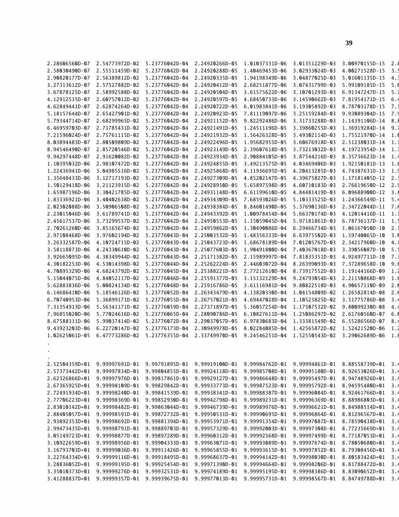
39
2.28606560D-07 2.54773972D-02 5.23776042D-04 2.24920266D-05 1.01037331D-06 3.01351229D-03 3.00970155D-15 2.80597530D-08
2.58030490D-07 2.55511459D-02 5.23776042D-04 2.24920288D-05 1.40469453D-06 3.02933024D-03 4.00271528D-15 3.54720923D-08
2.90820177D-07 2.56389812D-02 5.23776042D-04 2.24920335D-05 1.94198349D-06 3.04877025D-03 5.01601135D-15 4.30987061D-08
3.27313612D-07 2.57527882D-02 5.23776042D-04 2.24920412D-05 2.68251877D-06 3.07431799D-03 5.99109185D-15 5.05259754D-08
3.67878125D-07 2.58992588D-02 5.23776042D-04 2.24920504D-05 3.61575622D-06 3.10701293D-03 6.91347247D-15 5.76404781D-08
4.12912535D-07 2.60757012D-02 5.23776042D-04 2.24920597D-05 4.68450733D-06 3.14590662D-03 7.81954171D-15 6.46430358D-08
4.62849441D-07 2.62874264D-02 5.23776042D-04 2.24920722D-05 6.01983841D-06 3.19305892D-03 8.78703178D-15 7.19019678D-08
5.18157644D-07 2.65427901D-02 5.23776042D-04 2.24920923D-05 7.81119097D-06 3.25159284D-03 9.93089304D-15 7.97442175D-08
5.79344714D-07 2.68299965D-02 5.23776042D-04 2.24921152D-05 9.82292486D-06 3.31733288D-03 1.14391106D-14 8.83166301D-08
6.46959703D-07 2.71785431D-02 5.23776042D-04 2.24921491D-05 1.24511196D-05 3.39860255D-03 1.36919284D-14 9.75964259D-08
7.21596024D-07 2.75761115D-02 5.23776042D-04 2.24921932D-05 1.56426328D-05 3.49302114D-03 1.75521970D-14 1.07540055D-07
8.03894483D-07 2.80509809D-02 5.23776042D-04 2.24922496D-05 1.95682955D-05 3.60676918D-03 2.51238031D-14 1.18298671D-07
8.94546490D-07 2.85720546D-02 5.23776042D-04 2.24923149D-05 2.39607618D-05 3.73213032D-03 4.19723954D-14 1.30428544D-07
9.94297448D-07 2.91620082D-02 5.23776042D-04 2.24923934D-05 2.90884105D-05 3.87544216D-03 8.35736623D-14 1.45079788D-07
1.10395032D-06 2.98107472D-02 5.23776042D-04 2.24924855D-05 3.49213575D-05 4.03469406D-03 1.92150181D-13 1.64233387D-07
1.22436941D-06 3.04985516D-02 5.23776042D-04 2.24925868D-05 4.11936695D-05 4.20413285D-03 4.74387631D-13 1.91141372D-07
1.35648433D-06 3.12717193D-02 5.23776042D-04 2.24927309D-05 4.85202147D-05 4.39675827D-03 1.17181405D-12 2.31148228D-07
1.50129418D-06 3.21123915D-02 5.23776042D-04 2.24928950D-05 5.65897598D-05 4.60710183D-03 2.76619650D-12 2.92938236D-07
1.65987196D-06 3.30421785D-02 5.23776042D-04 2.24931148D-05 6.61199610D-05 4.84481419D-03 6.09688900D-12 3.89903762D-07
1.83336921D-06 3.40402638D-02 5.23776042D-04 2.24934309D-05 7.68593026D-05 5.10333525D-03 1.24366549D-11 5.40910584D-07
2.02302088D-06 3.50906508D-02 5.23776042D-04 2.24938384D-05 8.84601490D-05 5.37690136D-03 2.34722044D-11 7.69709237D-07
2.23015046D-06 3.61789741D-02 5.23776042D-04 2.24943392D-05 1.00978454D-04 5.66370174D-03 4.12014416D-11 1.10308624D-06
2.45617537D-06 3.73299557D-02 5.23776042D-04 2.24950553D-05 1.15059045D-04 5.97181861D-03 6.78736137D-11 1.56933466D-06
2.70261260D-06 3.85165674D-02 5.23776042D-04 2.24959862D-05 1.30490086D-04 6.29466734D-03 1.06167050D-10 2.19941392D-06
2.97108468D-06 3.97602194D-02 5.23776043D-04 2.25003532D-05 1.48356333D-04 6.63975502D-03 1.59740065D-10 3.03176426D-06
3.26332587D-06 4.10724715D-02 5.23776043D-04 2.25043723D-05 1.68678189D-04 7.01205767D-03 2.34217960D-10 4.11838410D-06
3.58118873D-06 4.24330610D-02 5.23776043D-04 2.25077603D-05 1.90491800D-04 7.40367018D-03 3.39056087D-10 5.52724084D-06
3.92665095D-06 4.38349944D-02 5.23776043D-04 2.25171382D-05 2.15989997D-04 7.81835351D-03 4.92497711D-10 7.33785060D-06
4.30182253D-06 4.53014398D-02 5.23776044D-04 2.25262224D-05 2.44603072D-04 8.26399093D-03 7.37289658D-10 9.63383418D-06
4.70895329D-06 4.68243792D-02 5.23776045D-04 2.25388221D-05 2.77212610D-04 8.73917552D-03 1.19144166D-09 1.25046924D-05
5.15044075D-06 4.84052117D-02 5.23776046D-04 2.25591377D-05 3.15132129D-04 9.24793054D-03 2.21150868D-09 1.60718254D-05
5.62883836D-06 5.00824134D-02 5.23776048D-04 2.25916786D-05 3.61116981D-04 9.80822518D-03 4.90657110D-09 2.05462229D-05
6.14686410D-06 5.18546126D-02 5.23776052D-04 2.26343479D-05 4.13820330D-04 1.04154809D-02 1.26582814D-08 2.63133330D-05
6.70740953D-06 5.36899171D-02 5.23776055D-04 2.26757021D-05 4.69447028D-04 1.10523825D-02 3.51775786D-08 3.40436196D-05
7.31354913D-06 5.56341171D-02 5.23776059D-04 2.27371897D-05 5.36057254D-04 1.17507532D-02 9.80099230D-08 4.48632530D-05
7.96855020D-06 5.77024616D-02 5.23776065D-04 2.28090786D-05 6.10827611D-04 1.25086297D-02 2.61760560D-07 6.06772196D-05
8.67588311D-06 5.99037414D-02 5.23776072D-04 2.29037057D-05 6.97830683D-04 1.33381549D-02 6.55286566D-07 8.47632214D-05
9.43923203D-06 6.22720147D-02 5.23776173D-04 2.30949978D-05 8.02284085D-04 1.42565872D-02 1.52421520D-06 1.22686621D-04
1.02625061D-05 6.47773286D-02 5.23776355D-04 2.33749970D-05 9.24546251D-04 1.52550543D-02 3.29062689D-06 1.83424421D-04
.
.
.
2.52504359D+01 9.99997691D-01 9.99791895D-01 9.99919100D-01 9.99984762D-01 9.99994861D-01 8.88558739D+01 3.47085480D+01
2.57373442D+01 9.99997834D-01 9.99804855D-01 9.99924118D-01 9.99985708D-01 9.99995180D-01 8.92653026D+01 3.47895810D+01
2.62326866D+01 9.99997976D-01 9.99817861D-01 9.99929127D-01 9.99986648D-01 9.99995497D-01 8.94748926D+01 3.48347360D+01
2.67365925D+01 9.99998109D-01 9.99829842D-01 9.99933773D-01 9.99987523D-01 9.99995792D-01 8.94595480D+01 3.48384430D+01
2.72491934D+01 9.99998240D-01 9.99841539D-01 9.99938341D-01 9.99988387D-01 9.99996084D-01 8.92461766D+01 3.48051802D+01
2.77706223D+01 9.99998369D-01 9.99852930D-01 9.99942798D-01 9.99989231D-01 9.99996369D-01 8.88986803D+01 3.47471501D+01
2.83010142D+01 9.99998482D-01 9.99863044D-01 9.99946739D-01 9.99989976D-01 9.99996621D-01 8.84988514D+01 3.46807208D+01
2.88405057D+01 9.99998591D-01 9.99872732D-01 9.99950531D-01 9.99990695D-01 9.99996864D-01 8.81296567D+01 3.46227975D+01
2.93892353D+01 9.99998692D-01 9.99881394D-01 9.99953971D-01 9.99991354D-01 9.99997087D-01 8.78590438D+01 3.45870198D+01
2.99473435D+01 9.99998791D-01 9.99889703D-01 9.99957329D-01 9.99992003D-01 9.99997308D-01 8.77235669D+01 3.45800664D+01
3.05149723D+01 9.99998877D-01 9.99897289D-01 9.99960312D-01 9.99992568D-01 9.99997499D-01 8.77187053D+01 3.45997071D+01
3.10922659D+01 9.99998956D-01 9.99904333D-01 9.99963071D-01 9.99993089D-01 9.99997674D-01 8.78050680D+01 3.46364019D+01
3.16793703D+01 9.99999036D-01 9.99911426D-01 9.99965855D-01 9.99993615D-01 9.99997852D-01 8.79308456D+01 3.46782759D+01
3.22764334D+01 9.99999116D-01 9.99918495D-01 9.99968637D-01 9.99994142D-01 9.99998030D-01 8.80583424D+01 3.47167856D+01
3.28836052D+01 9.99999195D-01 9.99925454D-01 9.99971390D-01 9.99994664D-01 9.99998206D-01 8.81788472D+01 3.47498177D+01
3.35010373D+01 9.99999276D-01 9.99932531D-01 9.99974189D-01 9.99995195D-01 9.99998386D-01 8.83090652D+01 3.47808926D+01
3.41288837D+01 9.99999357D-01 9.99939675D-01 9.99977013D-01 9.99995731D-01 9.99998567D-01 8.84749788D+01 3.48157464D+01

40
3.47673003D+01 9.99999431D-01 9.99946225D-01 9.99979579D-01 9.99996216D-01 9.99998730D-01 8.86945560D+01 3.48586667D+01
3.54164448D+01 9.99999492D-01 9.99951647D-01 9.99981716D-01 9.99996620D-01 9.99998867D-01 8.89673580D+01 3.49102395D+01
3.60764773D+01 9.99999548D-01 9.99956612D-01 9.99983663D-01 9.99996988D-01 9.99998991D-01 8.92734127D+01 3.49669810D+01
3.67475597D+01 9.99999605D-01 9.99961660D-01 9.99985642D-01 9.99997362D-01 9.99999117D-01 8.95814586D+01 3.50228427D+01
3.74298563D+01 9.99999658D-01 9.99966529D-01 9.99987536D-01 9.99997717D-01 9.99999237D-01 8.98665411D+01 3.50725760D+01
3.81235332D+01 9.99999709D-01 9.99971183D-01 9.99989326D-01 9.99998051D-01 9.99999349D-01 9.01340908D+01 3.51164365D+01
3.88287589D+01 9.99999757D-01 9.99975591D-01 9.99991035D-01 9.99998372D-01 9.99999457D-01 9.04412945D+01 3.51645085D+01
3.95457040D+01 9.99999797D-01 9.99979120D-01 9.99992422D-01 9.99998634D-01 9.99999545D-01 9.09022995D+01 3.52380540D+01
4.02745413D+01 9.99999835D-01 9.99982511D-01 9.99993757D-01 9.99998887D-01 9.99999631D-01 9.16673414D+01 3.53658742D+01
4.10154458D+01 9.99999861D-01 9.99984842D-01 9.99994661D-01 9.99999057D-01 9.99999688D-01 9.28771391D+01 3.55757544D+01
4.17685948D+01 9.99999884D-01 9.99986918D-01 9.99995461D-01 9.99999206D-01 9.99999738D-01 9.46077459D+01 3.58837330D+01
4.25341677D+01 9.99999905D-01 9.99988887D-01 9.99996222D-01 9.99999350D-01 9.99999787D-01 9.68316641D+01 3.62860702D+01
4.33123465D+01 9.99999917D-01 9.99990029D-01 9.99996647D-01 9.99999427D-01 9.99999813D-01 9.94224213D+01 3.67592029D+01
4.41033154D+01 9.99999926D-01 9.99991027D-01 9.99997000D-01 9.99999490D-01 9.99999833D-01 1.02215175D+02 3.72703226D+01
4.49072607D+01 9.99999935D-01 9.99992041D-01 9.99997358D-01 9.99999553D-01 9.99999854D-01 1.05104377D+02 3.77953354D+01
4.57243715D+01 9.99999945D-01 9.99993072D-01 9.99997723D-01 9.99999617D-01 9.99999875D-01 1.08125895D+02 3.83346686D+01
4.65548390D+01 9.99999954D-01 9.99994119D-01 9.99998093D-01 9.99999682D-01 9.99999897D-01 1.11462511D+02 3.89157330D+01
4.73988570D+01 9.99999964D-01 9.99995184D-01 9.99998470D-01 9.99999749D-01 9.99999919D-01 1.15346593D+02 3.95770730D+01
4.82566216D+01 9.99999973D-01 9.99996160D-01 9.99998818D-01 9.99999811D-01 9.99999939D-01 1.19899427D+02 4.03408931D+01
4.91283315D+01 9.99999976D-01 9.99996490D-01 9.99998929D-01 9.99999830D-01 9.99999945D-01 1.24999869D+02 4.11899955D+01
5.00141878D+01 9.99999978D-01 9.99996699D-01 9.99998993D-01 9.99999840D-01 9.99999949D-01 1.30270697D+02 4.20644479D+01
5.09143943D+01 9.99999979D-01 9.99996911D-01 9.99999058D-01 9.99999850D-01 9.99999952D-01 1.35201864D+02 4.28814892D+01
5.18291572D+01 9.99999980D-01 9.99997127D-01 9.99999124D-01 9.99999861D-01 9.99999955D-01 1.39342009D+02 4.35672431D+01
5.27586853D+01 9.99999982D-01 9.99997346D-01 9.99999190D-01 9.99999871D-01 9.99999959D-01 1.42449596D+02 4.40820116D+01
5.37031902D+01 9.99999983D-01 9.99997569D-01 9.99999258D-01 9.99999882D-01 9.99999962D-01 1.44531678D+02 4.44269887D+01
5.46628859D+01 9.99999985D-01 9.99997795D-01 9.99999327D-01 9.99999893D-01 9.99999966D-01 1.45776130D+02 4.46332392D+01
5.56379892D+01 9.99999987D-01 9.99998025D-01 9.99999397D-01 9.99999904D-01 9.99999969D-01 1.46439495D+02 4.47432143D+01
5.66287197D+01 9.99999988D-01 9.99998258D-01 9.99999469D-01 9.99999915D-01 9.99999973D-01 1.46754794D+02 4.47955002D+01
5.76352994D+01 9.99999990D-01 9.99998495D-01 9.99999541D-01 9.99999927D-01 9.99999977D-01 1.46888372D+02 4.48176571D+01
5.86579535D+01 9.99999991D-01 9.99998736D-01 9.99999615D-01 9.99999939D-01 9.99999980D-01 1.46938785D+02 4.48260211D+01
5.96969097D+01 9.99999993D-01 9.99998981D-01 9.99999689D-01 9.99999951D-01 9.99999984D-01 1.46955718D+02 4.48288311D+01
6.07523986D+01 9.99999995D-01 9.99999230D-01 9.99999765D-01 9.99999963D-01 9.99999988D-01 1.46960773D+02 4.48296701D+01
6.18246535D+01 9.99999996D-01 9.99999483D-01 9.99999842D-01 9.99999975D-01 9.99999992D-01 1.46962112D+02 4.48298923D+01
6.29139109D+01 9.99999998D-01 9.99999739D-01 9.99999920D-01 9.99999987D-01 9.99999996D-01 1.46962425D+02 4.48299444D+01
6.40204100D+01 1.00000000D+00 1.00000000D+00 1.00000000D+00 1.00000000D+00 1.00000000D+00 1.46962491D+02 4.48299553D+01
6.45780000D+01 1.00000000D+00 1.00000000D+00 1.00000000D+00 1.00000000D+00 1.00000000D+00 1.46962504D+02 4.48299575D+01
Finally, output filekvsgqh2o-0p-2000K.dat contains quadraturek-values as:wq gq kq aq1 aq2 aq3 aq4
5.5566E-02 5.1201E-02 5.9557E-06 1.0713E-05 2.8765E-04 3.7607E-02 3.3650E-01
7.5768E-02 1.1707E-01 3.0652E-05 9.0515E-04 1.7305E-02 1.5146E-01 5.1509E-01
9.2583E-02 2.0159E-01 8.3629E-05 3.7042E-03 6.8805E-02 3.7448E-01 7.1667E-01
1.0483E-01 3.0071E-01 2.0903E-04 8.4816E-03 1.4184E-01 6.0271E-01 8.8591E-01
1.1185E-01 4.0950E-01 4.7499E-04 3.1245E-02 2.1830E-01 7.2946E-01 9.6025E-01
1.1326E-01 5.2253E-01 9.5418E-04 1.3942E-01 3.9171E-01 8.7984E-01 1.0276E+00
1.0900E-01 6.3413E-01 1.8796E-03 4.1669E-01 7.4426E-01 1.1204E+00 1.1277E+00
9.9278E-02 7.3871E-01 3.7573E-03 8.5589E-01 1.2549E+00 1.4217E+00 1.2473E+00
8.4579E-02 8.3102E-01 7.5619E-03 1.6143E+00 1.9475E+00 1.7059E+00 1.3438E+00
6.5640E-02 9.0645E-01 1.6421E-02 3.2433E+00 3.0438E+00 2.0320E+00 1.4274E+00
4.3413E-02 9.6121E-01 4.3108E-02 6.5671E+00 4.6979E+00 2.4223E+00 1.5134E+00
1.9048E-02 9.9256E-01 1.9786E-01 1.5906E+01 8.1579E+00 3.0075E+00 1.6353E+00
Note that the code has an accuracy-checking mechanism built in: if the absorption coefficient is calcu-lated from the HITRAN/HITEMP databases, the Planck-mean absorption coefficient is calculated directlyfrom the database’s line intensities, equation (10.151), as well as by line-by-line integration of the absorptioncoefficient, equation (10.149): if the discrepancy exceeds 0.5% a message is printed to the screen, warningthatwvnst is too coarse to properly resolve the absorption coefficient. The Planck-mean absorption coef-ficient is also calculated from thek-g-distribution. Again, if the discrepancy exceeds 0.5% a message is
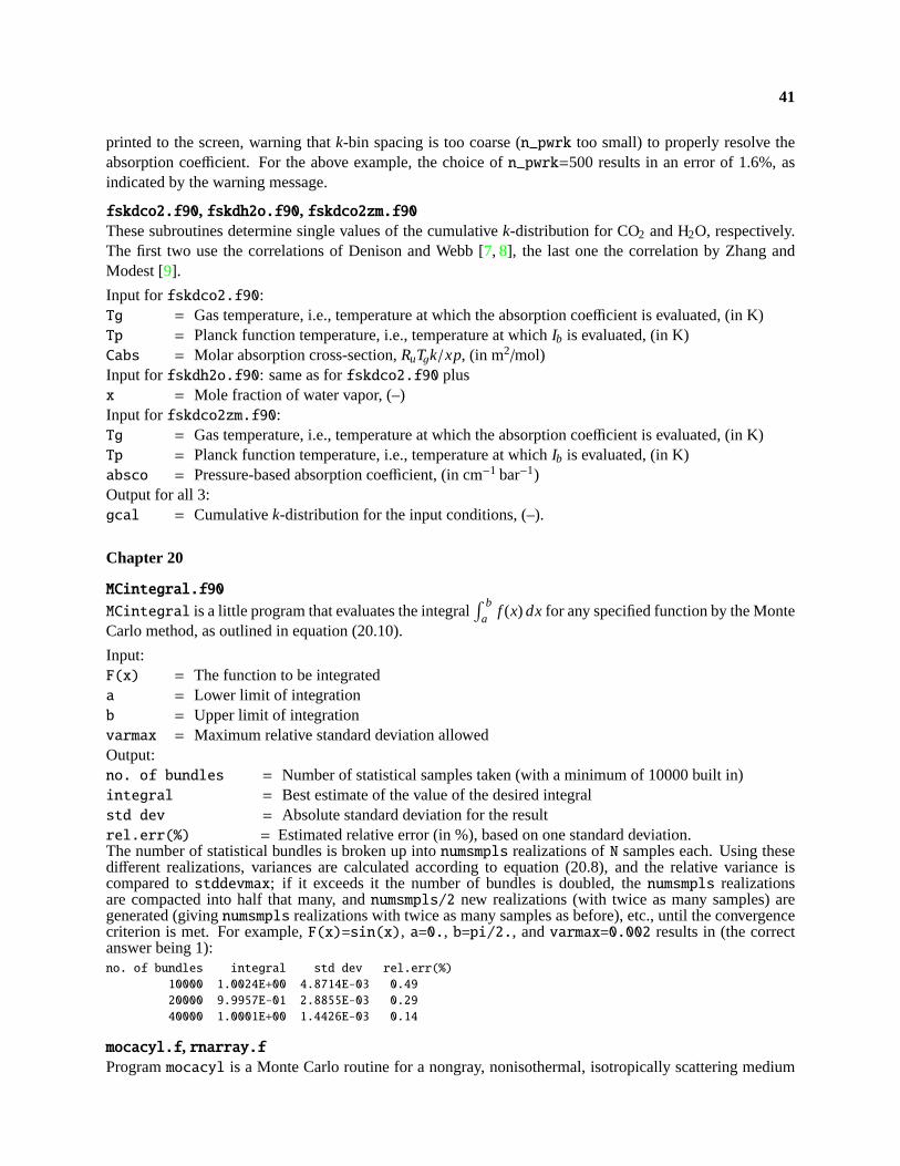
41
printed to the screen, warning thatk-bin spacing is too coarse (n_pwrk too small) to properly resolve theabsorption coefficient. For the above example, the choice ofn_pwrk=500 results in an error of 1.6%, asindicated by the warning message.
fskdco2.f90, fskdh2o.f90, fskdco2zm.f90These subroutines determine single values of the cumulativek-distribution for CO2 and H2O, respectively.The first two use the correlations of Denison and Webb [7, 8], the last one the correlation by Zhang andModest [9].
Input forfskdco2.f90:Tg = Gas temperature, i.e., temperature at which the absorption coefficient is evaluated, (in K)Tp = Planck function temperature, i.e., temperature at whichIb is evaluated, (in K)Cabs = Molar absorption cross-section,RuTgk/xp, (in m2/mol)Input forfskdh2o.f90: same as forfskdco2.f90 plusx = Mole fraction of water vapor, (–)Input forfskdco2zm.f90:Tg = Gas temperature, i.e., temperature at which the absorption coefficient is evaluated, (in K)Tp = Planck function temperature, i.e., temperature at whichIb is evaluated, (in K)absco = Pressure-based absorption coefficient, (in cm−1 bar−1)Output for all 3:gcal = Cumulativek-distribution for the input conditions, (–).
Chapter 20
MCintegral.f90
MCintegral is a little program that evaluates the integral∫ b
af (x) dx for any specified function by the Monte
Carlo method, as outlined in equation (20.10).
Input:F(x) = The function to be integrateda = Lower limit of integrationb = Upper limit of integrationvarmax = Maximum relative standard deviation allowedOutput:no. of bundles = Number of statistical samples taken (with a minimum of 10000 built in)integral = Best estimate of the value of the desired integralstd dev = Absolute standard deviation for the resultrel.err(%) = Estimated relative error (in %), based on one standard deviation.The number of statistical bundles is broken up intonumsmpls realizations ofN samples each. Using thesedifferent realizations, variances are calculated according to equation (20.8), and the relative variance iscompared tostddevmax; if it exceeds it the number of bundles is doubled, thenumsmpls realizationsare compacted into half that many, andnumsmpls/2 new realizations (with twice as many samples) aregenerated (givingnumsmpls realizations with twice as many samples as before), etc., until the convergencecriterion is met. For example,F(x)=sin(x), a=0., b=pi/2., andvarmax=0.002 results in (the correctanswer being 1):no. of bundles integral std dev rel.err(%)
10000 1.0024E+00 4.8714E-03 0.49
20000 9.9957E-01 2.8855E-03 0.29
40000 1.0001E+00 1.4426E-03 0.14
mocacyl.f, rnarray.fProgrammocacyl is a Monte Carlo routine for a nongray, nonisothermal, isotropically scattering medium
42
confined inside a two-dimensional, axisymmetric cylindrical enclosure bounded by gray, diffusely emit-ting and reflecting walls. Temperature and radiative properties are assumed known everywhere inside theenclosure and along the walls. Requires use of programrnarray to set up random number relationships(locations and wavenumbers of emission vs. random numbers). Calculates local radiative fluxes to the wallsqRw. mocacyl.f is supplied in two slightly different versions:mocacyl_std.f uses standard Monte Carlo
for absorption, i.e., an absorption length is picked from equation (20.70) and the bundle is traced until thispoint is reached (and its energy is deposited at that point) or to a point on a wall, where it is absorbed (i.e.,picking a random numberRα < α), whichever comes first. In the other version,mocacyl_ep.f, the energypartitioning scheme of Section 20.10 is employed, i.e., the bundle’s energy is gradually attenuated by ab-sorption along its path, and by the fractionα, whenever the bundle hits (and is reflected from) a wall, untilthe bundles energy becomes negligible. This method is somewhat more expensive per bundle, but shouldin many instances give converged results with a lot less bundles. At the present time onlymocacyl_std.f
also calculates the internal radiative source−∇ · qR in addition to wall fluxes.The package consists of the following files:
• the main programsmocacyl_std.f andmocacyl_ep.f ,
• the program preparing random number relationships for medium emission,rnarray.f,
• file mocasub.f, which contains simple versions of subroutinePROPS and functionABSCO, as well asa poor man’s random number generator calledRNUM, all of which the user can (and should) replace,
• a filesplines.f for monotonic splines,used by bothmocacyl.f andrnarray.f, and
• sample output filesdatlam.dat andresults.dat.
The documentation for these two routines is not yet complete and will be updated.ProgramrnarrayThis program prepares random number relationships for photon emission locations within the cylindricalmedium, using equations (20.62) and (20.64).Input:NRP = Number of radial nodes for medium emission random number relationshipsNZP = Number of axial nodes for medium emission random number relationshipsNNP = Number of random numbers for medium emission relationshipsRL = Radius of cylinder, (cm)ZL = Length of cylinder, (cm)AN = Refractive index of medium (AN=1.0 for gases)STN = Refractive index of sootSTK = Absorptive index of sootIGRAY = Gray/nongray medium switch:IGRAY=0 nongray,IGRAY=1 gray (ignoring contribution from
gases; absorption coefficient= PAC)LU = Logical unit number for output:LU=6 sends output to screen, other (legal) values send output
to file datlam.datOutput:File datlam.dat contains random number relationships generated byRNARRAY:ETOTAL = Total energy emitted (per unit time) by entire volume, in WPLMCL(I),I=1,NZP = Planck-mean absorption coefficient along centerline, in cm−1
RRA(J),J=1,NNP = Emission radial location asf (random#), in cmZR(K,J),K=1,NRP,J=1,NNP = Emission axial location asf (r, random#), in cmWVE2(K,I,J),K=1,NRP,I=1,NZP,J=1,NRNP1 = Emission wavelength asf (r, z, random#) (IGRAY=0
only), in µm
43
These arrays are used bymocacyl.f to determine emission location and wavelength, using single (r),double (z), and triple (λ) linear interpolation between tabulated values.
Note: this program requires two user-supplied subroutines,SUBROUTINE PROPS andFUNCTION ABSCO.SubroutinePROPS(R,Z,T,SVF,PCO2,PH2O,PAC,PSC), upon inputting radial positionR (in cm) and axialpositionZ (in cm), must return local values ofT (temperature in K),SVF (soot volume fraction, –),PCO2(partial pressure of CO2, in bar),PH2O (partial pressure of H2O, in bar),PAC (nonsoot particle background ab-sorption coefficient, in cm−1), andPSC (nonsoot particle background scattering coefficient, in cm−1). As pro-vided here, the subroutine produces a uniform field, i.e.,SVF=0., T=1000., PH2O=.1, PCO2=.1, PAC=.01,
PSC=0.
FunctionABSCO(SVF,PCO2,PH2O,PAC,W,T), upon inputtingSVF (soot volume fraction, –),PCO2 (partialpressure of CO2, in bar),PH2O (partial pressure of H2O, in bar),PAC (nonsoot particle background absorptioncoefficient, in cm−1), W (wavelength inµm), andT (temperature in K), must returnABSCO, the absorptioncoefficient of the medium (in cm−1). As provided, functionABSCO calculates the gas absorption coefficientfrom the wide-band model [with an approximate evaluation ofα(T)/α0 in equation (10.111)] assumingstrong overlap (β→ ∞), and the soot absorption coefficient is calculated from equation (11.124).FunctionABSCO should returnABSCO=PAC if W < 0 (gray medium). Both,PROPS andABSCO, must containthe common statement lineCOMMON RL,ZL,AN,STN,STK,NRR,NZL,NRN.
ProgrammocacylProgrammocacyl requires the following input:NRP = Number of radial nodes for medium emission random number relationshipsNZP = Number of axial nodes for medium emission random number relationshipsNNP = Number of random numbers for medium emission relationshipsNR = Number of radial nodes for surface flux calculationsNZ = Number of axial nodes for surface flux calculationsT3(NZ) = Temperature of liner wall (r = R), (K)EPS(3) = Surface emittances:EPS(1)=inlet, EPS(2)=exit, EPS(3)=linerRL = Radius of cylinder, (cm)ZL = Length of cylinder, (cm)AN = Refractive index of medium (AN=1.0 for gases)STN = Refractive index of sootSTK = Absorptive index of sootNTOTAL = Total number of photon bundles emitted from medium (number of bundles for surface emission
are chosen automatically as function ofNTOTAL)IGRAY = Gray/nongray medium switch:IGRAY=0 nongray,IGRAY=1 gray (ignoring contribution from
gases and soot; absorption coefficient= PAC)IWALL = Wall emission switch:IWALL=0 only considers medium emission;IWALL=1 also considers
surface emissionLU = Logical unit number for output:LU=6 sends output to screen, other (legal) values send output
to file results.datFile datlam.dat Contains random number relationships generated byrnarray
Note: The programdoes not checkfor consistency ofdatlam.dat, i.e., whether identical input valueshave been chosen in bothrnarray andmocacyl!
Output:Upon output relevant input data are displayed, as well asQW(1,1..NR) = Axial radiative heat flux forNR radial nodes at inlet (W/cm2)QW(2,1..NR) = Axial radiative heat flux forNR radial nodes at exit (W/cm2)QW(3,1..NZ) = Radial radiative heat flux forNZ axial nodes at liner (W/cm2)Note: QW > 0 implies that the flux goes into wall, while forQW < 0 the flux is out of the wall.
Example:We will use routinesPROPS andABSCO as provided, and also the input data as stated inmocacyl (and similarin rnarray):C C GENERAL DATA C C T3=liner temperature (K),

44
EPS=emittances(inlet,exit,liner), C RL=radius (cm), ZL=length (cm),
AN=refractive index of medium (-), C STN= soot refractive index, STK= soot
absorptive index, C NRR=# radial nodes, NZL=# axial nodes, NRN=# wavelength
nodes C
DATA T3/7*1000./
DATA EPS/1.,1.,.5/
RL=10.
ZL=10.
TW0=1000.
TWL=0.
AN=1.
STN=1.89
STK=0.92
NTOTAL=500000
IGRAY=0
IWALL=1
LU=7
This models an isothermal, cylindrical, nongray medium with temperatures of 1000 K for medium, inletand liner, only the exit being cold at 0 K. For the simulation we will use 500,000 bundles for mediumemission, and corresponding numbers for surface emission (such that all bundles carry roughly identicalenergies). Executingrnarray produces the required data filedatlam.dat and, runningmocacyl, theresults are contained inresults.dat as:
GENERAL DATA
************
BURNER RADIUS 10.00 CM
BURNER LENGTH 10.00 CM
EMITTANCES: INLET: 1.00
EXIT: 1.00
LINER: 0.50
REFRACTIVE INDEX 1.00
NUMBER OF BUNDLES: MEDIUM: 500000
INLET: 474561
EXIT: 1
LINER: 474562
WALL TEMPERATURES (DEG.K)
TW0 TWL T3:I= 1 2 3 4 5 6 7
1000. 0. 1000. 1000. 1000. 1000. 1000. 1000. 1000.
PROPERTY VALUES ALONG CENTER LINE:
I Z T FR PCO2 PH2O K-PL ABSC SCAT
CM DEG.K % ATM ATM CM-1 CM-1 CM-1
1 0.0 1000. 0.00 0.100 0.100 0.032 0.010 0.000
2 0.5 1000. 0.00 0.100 0.100 0.032 0.010 0.000
3 1.0 1000. 0.00 0.100 0.100 0.032 0.010 0.000
4 1.5 1000. 0.00 0.100 0.100 0.032 0.010 0.000
5 2.0 1000. 0.00 0.100 0.100 0.032 0.010 0.000
6 2.5 1000. 0.00 0.100 0.100 0.032 0.010 0.000
7 3.0 1000. 0.00 0.100 0.100 0.032 0.010 0.000
8 3.5 1000. 0.00 0.100 0.100 0.032 0.010 0.000

45
9 4.0 1000. 0.00 0.100 0.100 0.032 0.010 0.000
10 4.5 1000. 0.00 0.100 0.100 0.032 0.010 0.000
11 5.0 1000. 0.00 0.100 0.100 0.032 0.010 0.000
12 5.5 1000. 0.00 0.100 0.100 0.032 0.010 0.000
13 6.0 1000. 0.00 0.100 0.100 0.032 0.010 0.000
14 6.5 1000. 0.00 0.100 0.100 0.032 0.010 0.000
15 7.0 1000. 0.00 0.100 0.100 0.032 0.010 0.000
16 7.5 1000. 0.00 0.100 0.100 0.032 0.010 0.000
17 8.0 1000. 0.00 0.100 0.100 0.032 0.010 0.000
18 8.5 1000. 0.00 0.100 0.100 0.032 0.010 0.000
19 9.0 1000. 0.00 0.100 0.100 0.032 0.010 0.000
20 9.5 1000. 0.00 0.100 0.100 0.032 0.010 0.000
21 10.0 1000. 0.00 0.100 0.100 0.032 0.010 0.000
RADIAL HEAT FLUXES AT NODES I (W/SQCM)
I Z QWALL
CM W/SQCM
1 0.7 -0.4
2 2.1 -0.4
3 3.6 -0.5
4 5.0 -0.7
5 6.4 -0.8
6 7.9 -1.0
7 9.3 -1.2
AXIAL HEAT FLUXES AT NODES J (W/SQCM)
J 1 2 3 4 5
Q0 -2.4 -2.3 -2.1 -1.9 -1.6
QL 5.9 5.8 5.8 5.6 5.4
Note that the fluxes for the three hot walls are slightly negative (surfaces are losing heat, while the coldexit surface experiences strong positive heat fluxes. Also note that the code does not provide error estimates,i.e., it should be run for different values ofNTOTAL to get an idea of variances.
FwdMCcs.f90
ProgramFwdMCcs is a standard forward Monte Carlo code for a narrow collimated, cylindrical beam (cen-tered atx = y = 0) penetrating through a nonabsorbing, isotropically scattering slab, calculating the fluxonto a small, directionally-selective detector located atx0 < x < x0 + dx, 0 < y < dy, z = L, as shown inFig. 20-10 and described in Example 20.6. (FwdMCck1 andFwdMCck2 are forward Monte Carlo codes forthe same problem, but also allow for absorption in the medium;FwdMCck1 uses standard ray tracing, whileFwdMCck2 uses energy partitioning; see Example 20.7.)
Input:L = thickness of layer,L (m);sig = scattering coefficient of medium,σs (m−1);QT = total energy contained in collimated beam, (W);R = radius of collimated beam,R (m);x0 = displacement of left end of detector from center of beam,x0 (m);dx = width of detector inx-direction, (m);dy = width of detector iny-direction, (m);thd = opening angle of detector,θmax (degrees);
46
N = minimum number of photon bundles to be traced for each “sample;”numsmpl = number of numerical “samples” collected for the determination of a variance;stddevmax = maximum relative variance allowed for the calculation ofqdet, the flux hitting detector,
= σm/qdet from equation (20.8).The values for input parameters are assigned in sequence near the top of the program. As distributed, a
1 m thick layer with a scattering coefficient ofσs = 1m−1 is modeled, for a 10 cm radius beam of 100 Wstrength. The (rather large) detector is 10 cm× 10 cm displaced by 20 cm from the center of the beam, andhas an acceptance angle of 10. numsmpl= 10 numerical samples will be taken, initially each containingN= 100,000 bundles, to be increased (if necessary) until the relative variance falls belowstddevmax= 0.05or 5%.
open(unit=8,file=’fwdmccs.dat’,status=’unknown’)
write(8,1)
write(*,1)
1 format(’no. of bundles q_det variance rel.var.(%)’)
!
L=1. ! m
sig=1. ! 1/m
QT=100. ! W
R=.1 ! m
x0=.2 ! m
dx=0.10 ! m
dy=0.10 ! m
thd=10. ! deg
N=100000
numsmpl=10
stddevmax=0.05
!
The program consists of two major parts. The first is a double loop overnumsmpl*N photon bundles,tracing their paths, as described in Example 20.6. In the second part an average value for the detectorirradiation is determined, as well as its relative standard deviation, based on thenumsampl data points. Ifthe relative standard deviation is too large (stddev>stddevmax) thenumsampl samples ofqdet (based onN bundles) are combined into1/2×numsampl samples (with 2N bundles each), the number of bundles isdoubled to 2N , and an additional1/2×numsampl samples are obtained (with 2N bundles each). Thus, aftergoing through the bundle-tracing part one more time, we have againnumsmpl samples, but each based ontwice as many photon bundles. This procedure is repeated until the convergence criteria are met.
For the given case that leads to the following output, stored infwdmccs.dat,no. of bundles q_det variance rel.var.(%)
1000000 0.3200E-02 0.4899E-03 15.31
2000000 0.3500E-02 0.3944E-03 11.27
4000000 0.3100E-02 0.3055E-03 9.86
8000000 0.2963E-02 0.1468E-03 4.95
i.e., for this large detector 8,000,000 photon bundles are needed to attain a relative variance of less than 5%.If a smaller detector was chosen, the necessary number of bundles would be roughly inversely proportionalto the detector area!
FwdMCck1.f90
ProgramFwdMCck1.f90 is identical toFwdMCcs.f90, except that the medium also absorbs radiation (be-sides isotropically scattering it). Therefore, the input is:
Input:L = thickness of layer,L (m);sig = scattering coefficient of medium,σs (m−1);kap = absorption coefficient of medium,κ (m−1);QT = total energy contained in collimated beam, (W);
47
R = radius of collimated beam,R (m);x0 = displacement of left end of detector from center of beam,x0 (m);dx = width of detector inx-direction, (m);dy = width of detector iny-direction, (m);thd = opening angle of detector,θmax (degrees);N = minimum number of photon bundles to be traced for each “sample;”numsmpl = number of numerical “samples” collected for the determination of a variance;stddevmax = maximum relative variance allowed for the calculation ofqdet, the flux hitting detector,
= σm/qdet from equation (20.8).As distributed, a 1m thick layer with a scattering coefficient of 1m−1 and an absorption coefficient of
κ = 1m−1 is modeled, for a 10 cm radius beam of 100 W strength. The (rather large) detector is 10 cm×10 cm displaced by 20 cm from the center of the beam, and has an acceptance angle of 10. numsmpl=10 numerical samples will be taken, initially each containingN = 100,000 bundles, to be increased (ifnecessary) until the relative variance falls belowstddevmax = 0.05 or 5%:
open(unit=8,file=’fwdmck1.dat’,status=’unknown’)
write(8,1)
write(*,1)
1 format(’no. of bundles q_det variance rel.var.(%)’)
!
L=1. ! m
sig=1. ! 1/m
kap=1. ! 1/m
QT=100. ! W
R=.1 ! m
x0=.2 ! m
dx=0.10 ! m
dy=0.10 ! m
thd=10. ! deg
N=100000
numsmpl=10
stddevmax=0.05
!
For the given case that leads to the following output, stored infwdmck1.dat:no. of bundles q_det variance rel.var.(%)
1000000 0.1100E-02 0.2333E-03 21.21
2000000 0.7500E-03 0.2007E-03 26.76
4000000 0.6500E-03 0.1067E-03 16.42
8000000 0.6875E-03 0.7512E-04 10.93
16000000 0.6438E-03 0.4375E-04 6.80
32000000 0.6781E-03 0.4396E-04 6.48
64000000 0.6766E-03 0.3424E-04 5.06
128000000 0.7102E-03 0.3011E-04 4.24
i.e., 128,000,000 photon bundles are required, or – making allowance for the slightly different variance –about 10 times as many as for the purely scattering medium. Clearly, with a minimum optical thicknessof√
12 + 0.22 = 1.02 many photon bundles, that would otherwise be scattered toward the detector, becomeabsorbed first.
FwdMCck2.f90ProgramFwdMCck2.f90 is identical toFwdMCck1.f90, except that energy partitioning is employed, i.e.,photon bundles are emitted and have paths identical to the simulation inFwdMCcs.f90, but the bundles’strengths are attenuated exponentially along their way according to Beer’s law. Input is identical toFwdMCck1.f90,as are the as-distributed input parameters. However, the output (stored infwdmck2.dat) now looks like this:no. of bundles q_det variance rel.var.(%)
1000000 0.9003E-03 0.1610E-03 17.89
2000000 0.9382E-03 0.1109E-03 11.82
48
4000000 0.8160E-03 0.8774E-04 10.75
8000000 0.7927E-03 0.3710E-04 4.68
i.e.,FwdMCck2.f90 converges at he same rate as the no-absorption caseFwdMCcs.f90, demonstrating thepower of the energy partitioning approach.
FwdMCps.f90
ProgramFwdMCps is a standard forward Monte Carlo code for radiative energy emitted by a point sourcepenetrating through a nonabsorbing, isotropically scattering slab, calculating the flux onto a small, directionally-selective detector. It is a variation ofFwdMCcs.f90, considering a purely scattering slab, but replacing thecollimated beam by an internal point source atx = 0, y = 0, z= zps. Thus, the simulation is almost identicalto that ofFwdMCcs.f90, except that all photon bundles are now emitted from a single point, but into randomdirections. The input is also identical toFwdMCcs.f90, with R replaced byzps:
Input:L = thickness of layer,L (m);sig = scattering coefficient of medium,σs (m−1);QT = total energy contained in point source, (W);zps = z-coordinate of point source, (m);x0 = displacement of left end of detector from point source,x0 (m);dx = width of detector inx-direction, (m);dy = width of detector iny-direction, (m);thd = opening angle of detector,θmax (degrees);N = minimum number of photon bundles to be traced for each “sample;”numsmpl = number of numerical “samples” collected for the determination of a variance;stddevmax = maximum relative variance allowed for the calculation ofqdet, the flux hitting detector,
= σm/qdet from equation (20.8).The as-delivered case also is the same as forFwdMCcs.f90, with the 10 cm-radius beam replaced by a
points source atzps = 0.5(m). Thus, the input section reads:open(unit=8,file=’fwdmcps.dat’,status=’unknown’)
write(8,1)
write(*,1)
1 format(’no. of bundles q_det variance rel.var.(%)’)
!
L=1. ! m
sig=1. ! 1/m
QT=100. ! W
zps=.1 ! m
x0=.2 ! m
dx=0.10 ! m
dy=0.10 ! m
thd=10. ! deg
N=100000
numsmpl=10
stddevmax=0.05
!
The resulting output, stored infwdmcps.dat, is:no. of bundles q_det variance rel.var.(%)
1000000 0.5000E-02 0.7303E-03 14.61
2000000 0.4550E-02 0.4561E-03 10.02
4000000 0.4800E-02 0.3958E-03 8.25
8000000 0.4850E-02 0.3226E-03 6.65
16000000 0.4850E-02 0.2143E-03 4.42
RevMCcs.f90
This program is a reverse or backward Monte Carlo implementation of the problem solved byFwdMCcs.f90,

49
i.e., a narrow collimated beam hitting a purely scattering slab, and scattered toward a small, directionally-selective detector. Input and output are identical toFwdMCcs, except that the default minimum number ofphoton bundles is much smaller, here set toN=1000.
Again, the program consists of two parts, a double loop tracing overnumsmpl×N photon bundles, and amodule calculating detector power and its standard deviation. Tracing follows the rules of equation (20.108),and the detector flux from equation (20.104) (withε
′
λ = 1 for the black detector). The coding is self-explanatory except when, between two scattering events, the bundle starts and ends outside the collimatedbeam column,x2 + y2 = r2 > R2. There are four different possibilities, as illustrated in the sketch below:
( )x ,yi i
case
(1)
case
(3)
case
(2)
case
(4)
R
Öd
( )x ,yi i
( )x ,yi i
( )x ,yi i
( )x ,ye e
( )x ,ye e
( )x ,ye e
( )x ,ye e
(0,0)
1. The path of the bundle misses the beam altogether,
2. the path intercepts the beam, but the bundle is moving away from the beam,
3. the path intercepts the beam and moves toward it, but is scattered anew before reaching it, and finally
4. the bundles path intersects the beam.
These four possibilities are tested by calculating the partial distancesl1 and l2 (lpart) from the startingpoint (projected into thex-y-plane) (xi , yi) toward (xe, ye) (the final point) to where the path enters and exitsthe beam. Thus, using thex- andy-components of the vector equation
r i + ls= R
leads toxi + lsx = xc,
yi + lsy = yc,
where (xc, yc) is a point on the outer limit of the collimated beam,r = R. Squaring and adding the latter twoequations gives
x2i + y
2i + 2(xi sx + yi sy)l + (s2
x + s2y )l
2 = R2
or
l1,2 =−b±
√d
c,
where
a = x2i + y
2i − R2
b = xi sx + yi sy
c = s2x + s2
y
d = b2 − ac.
50
Thus the above four scenarios correspond to
1. If d < 0 the roots are complex, i.e., there is no intersection,
2. If l1 < 0 the bundle moves away from beam
3. If l1 < lσ the bundle is scattered again before reaching the beam, and
4. otherwise both intercepts are calculated to determineIλn.
After the tracing of photon bundles is completed, average values and standard deviations are calculatedas in the forward Monte Carlo codes, e.g.,FwdMCcs. Using the as-supplied input (same as forFwdMCcs, butwith N=1000) leads to the output, stored inrevmccs.dat:no. of bundles q_det variance rel.var.(%)
10000 0.2882E-02 0.1192E-03 4.14
Thus, a better variance is achieved with only 10,000 bundles, as opposed to the 8,000,000 bundles usedin the forward simulation (and this ratio would become correspondingly more extreme for smaller detectorareas and acceptance angles).
RevMCck1.f90, RevMCck2.f90These programs are backward Monte Carlo Implementations ofFwdMCck1 andFwdMCck2, respectively, asalso discussed in Example 20.7. They have identical inputs (except the much lower minimum number ofphoton bundles, here set toN=1000 as default); and their outputs also follow the format of their counterparts.Ray tracing forRevMCck1 is the same as forRevMCcs, except for the slight modification demanded byequation (20.109). If energy partitioning is used, attenuation along the entire path length of the photonbundle must be considered, as explained in the last equation of Example 20.7. For the as-supplied cases theoutput fromRevMCck1, stored inrevmck1.dat, is:no. of bundles q_det variance rel.var.(%)
10000 0.7261E-03 0.5045E-04 6.95
20000 0.7540E-03 0.3091E-04 4.10
i.e., 20,000 bundles are required (as opposed to 128,000,000 used byFwdMCck1). ForRevMCck2 the output,stored inrevmck2.dat, is:no. of bundles q_det variance rel.var.(%)
10000 0.7623E-03 0.3061E-04 4.02
i.e., 10,000 bundles are required (as opposed to 8,000,000 used inFwdMCck2, or 20,000 used inRevMCck1).
RevMCps.f90
This program is the backward Monte Carlo equivalent ofFwdMCps, with identical input and output format(again, with the exception of a much smaller base line value for the number of bundles). In the backwardMonte Carlo simulation, the detector flux again consists of a direct and a scattered component. In the codeit is assumed that the direct component is zero, this time because all direct radiation hits the detector atan angle larger than the acceptance angle (this could, of course, be easily changed). As for collimatedirradiation backward Monte Carlo also becomes inefficient if the radiation source comes from a very smallsurface or volume. The trick is again to break up intensity into a direct component (intensity coming directlyfrom the source without scattering or wall reflections), and a multiply-scattered and reflected part, as givenby Modest [10] and briefly described here. Again, we letId satisfy the radiative transfer equation withoutthe inscattering term, or,
s · ∇Id(r , s) = Sd(r , s)− β(r )Id(r , s),
which has the simple solution
Id(r , s) =∫
Sd(r ′, s) exp
[−
∫r→r ′
(κ + σs) ds′]ds, (CC-43)
51
where the main integral is along a straight path from the boundary of the medium to pointr in the directionof s. For example, if there is only a simple point source atr0 with total strengthQ0, emitting isotropicallyacross a tiny volumeδV, equation (CC-43Chapter 20equation.CC-43) becomes
Id(r , s) =Q0
4π|r0 − r |2exp
[−
∫r0→r
(κ + σs) ds′]δ(s− s0), (CC-44)
wheres is a unit vector pointing fromr0 towardr , and use has been made of the fact that
δV = δAδs= δΩ0|r0 − r |2 δs,
whereδΩ0 is the solid angle, with whichδV is seen fromr. Equation (CC-44Chapter 20equation.CC-44)can be used to calculate the direct contribution ofQ0 hitting a detector, and it can be used to determine thesource term for the RTE of the scattered radiation as
S1(r , s) =σs(r )4π
∫4π
Id(r , s′)Φ(r , s′, s) dΩ′
=σs(r )Q0
16π2|r0 − r |2exp
[−
∫r0→r
(κ + σs)ds′]Φ(r, s0, s). (CC-45)
The rest of the solution proceeds as before, withIn(r i ,− si) found from equations (CC-45Chapter 20equation.CC-45)and (20.107) as
In (r i ,−si) =σsQ
16π2
∑j
∫lσ, j
e−σs|r0−r |
|r0 − r |2dl′, (CC-46)
where thelσ, j are the straight paths the bundle travels between scattering events. Equation (CC-46Chapter20equation.CC-46) must be integrated numerically, and this can be done using a simple Newton-Cotesscheme. Alternatively, the integral can be obtained statistically from
In (r i ,−si) =σsQ
16π2
∑j
lσ, jNint
Nint∑k=1
e−σs|r0−rk|
|r0 − rk|2,
where therk areNint random locations chosen uniformly along pathlσ, j . This was implemented inRevMCps.f90,choosingNint (= numint) to be inversely proportional to the distance of the integration point from the source(or proportional to its relative importance). Results for detector flux for the as-supplied case (same as forFwdMCps.f90) are stored inrevmcps.dat as:no. of bundles q_det variance rel.var.(%)
10000 0.4614E-02 0.1057E-03 2.29
i.e., with only 10,000 bundles we achieved a much better variance then by using 16,000,000 bundles inFwdMCps.f90.
RevMCps.f90
The backward Monte Carlo equivalent ofFwdMCps.
The documentation for this routine is not yet complete and will be updated.
Third-Party Codes
MONT3D
This code, developed at Colorado State University by Burns et al. [11, 12, 13, 14, 15], calculates radiativeexchange factors for complicated, three-dimensional geometries by the Monte Carlo method, as given byequations (20.12) and (20.16). Diffuse and specular view factors may be calculated as special cases. We

52
provide here only a link to the Colorado State University web site, where documentation and codes are keptup-to-date:http://www.colostate.edu/˜pburns/monte.html
VIEW3D
This code, developed at National Institute of Standards and Technology (NIST) by Walton [16], calculatesradiative view factors with obstructions by adaptive integration. The package, as posted here, consists of 4files:
1. The official NIST publication (NISTIR-6925.pdf),
2. A compressed file containing the program executables, help files, etc. (v3d32exe.zip),
3. A compressed file containing the program documentation (V3D32doc.zip), and
4. A compressed file containing sample data files (IEA22dat.zip).
For problems with and/or feedback for this package please address them directly to the author, GeorgeWalton ([email protected]).
RADCAL
This code, developed at NIST by Grosshandler [17,18] is a narrow band database for combustion gas prop-erties, using tabulated values and theoretical approximations. The package consist of two files:
1. A user manual (NIST Technical NoteTN 1402.pdf), and
2. a compressed file containing the program Fortran file and sample input and output files (RADCAL.zip).
For problems with and/or feedback for this package please address them directly to the author, WilliamGrosshandler ([email protected]).
EM2C
This package contains a number of Fortran codes, developed at the Ecole Centrale de Paris by Soufianiand Taine [19], calculating statistical narrow band properties as well as narrow bandk-distributions forCO2 and H2O, using the HITRAN92 database together with some proprietary French high-temperatureextensions. The entire package is provided in the form of a compressed file containing the program For-tran files, data files and documentation (em2c.zip). For problems with and/or feedback for this packageplease address them directly to the authors, Anouar Soufiani ([email protected]) and/or Jean Taine([email protected]).
FVM2D
This Fortran77 code, developed at the University of Minnesota and Nanyang Technological University byChai and colleagues [20,21,22], calculates radiative transfer in participating media using the finite-volumemethod of Chapter 16 for a two-dimensional, rectangular enclosure with reflecting walls and an absorbing,emitting, anisotropically scattering medium. For each surface the emittance and blackbody intensities mustbe specified; for the medium spatial distributions of radiation properties and blackbody intensities must beinput. Calculated are internal incident radiation (G) and wall flux (q) fields. Can be used for gray problemsor on a spectral basis. The package consists of two files:
1. A user manual (RAT.pdf), and
2. a compressed file containing the program Fortran files (RATcode.zip).
Four modules are needed to runFVM2D. These arePARAM.FOR, COMMON.FOR, RATmain.FOR andADAPT.FOR.In this nomenclature,RATmain.FOR andADAPT.FOR are the invariant part and the adaptation portion of theprogram, respectively.COMMON.FOR contains all the common block related variables, whilePARAM.FORcontains the parameters for the program. These files are all contained inRATcode.zip, providing the 6
53
different versions ofADAPT.FOR corresponding to the 6 examples described in the manual. The manual asgiven is preliminary, i.e., two more examples dealing with irregular geometry and non-gray media, respec-tively, will be added at a later time.For problems with and/or feedback for this package please address them directly to the author, John (CheeKiong) Chai ([email protected]).
References
1. Humlıcek, J.: “Optimized computation of the Voigt and complex probability functions,”Journal of Quantitative Spec-troscopy and Radiative Transfer, vol. 27, p. 437, 1982.
2. Buckius, R. O., and D. C. Hwang: “Radiation properties for polydispersions: Application to coal,”ASME Journal of HeatTransfer, vol. 102, pp. 99–103, 1980.
3. Menguc, M. P., and R. Viskanta: “On the radiative properties of polydispersions: A simplified approach,”CombustionScience and Technology, vol. 44, pp. 143–159, 1985.
4. Hageman, L. A., and D. Young:Applied Iterative Methods, Academic Press, 1981.5. Wu, C. Y., and N. R. Ou: “Differential approximations for transient radiative transfer through a participating medium exposed
to collimated irradiation,”Journal of Quantitative Spectroscopy and Radiative Transfer, vol. 73, pp. 111–120, 2002.6. Ferziger, J. H.:Numerical Methods for Engineering Application, 2nd ed., John Wiley & Sons, New York, 1981.7. Denison, M. K., and B. W. Webb: “An absorption-line blackbody distribution function for efficient calculation of total gas
radiative transfer,”Journal of Quantitative Spectroscopy and Radiative Transfer, vol. 50, pp. 499–510, 1993.8. Denison, M. K., and B. W. Webb: “Development and application of an absorption line blackbody distribution function for
CO2,” International Journal of Heat and Mass Transfer, vol. 38, pp. 1813–1821, 1995.9. Zhang, H., and M. F. Modest: “Full-spectrumk-distribution correlations for carbon dioxide mixtures,” inProceedings of the
2002 AIAA/ASME Thermophysics Conference, 2002.10. Modest, M. F.: “Backward Monte Carlo simulations in radiative heat transfer,”ASME Journal of Heat Transfer, vol. 125,
no. 1, pp. 57–62, 2003.11. Burns, P. J.: “MONTE–a two-dimensional radiative exchange factor code,” Technical report, Colorado State University, Fort
Collins, 1983.12. Maltby, J. D.: “Three-dimensional simulation of radiative heat transfer by the Monte Carlo method,” M.S. thesis, Colorado
State University, Fort Collins, CO, 1987.13. Burns, P. J., and J. D. Maltby: “Large-scale surface to surface transport for photons and electrons via Monte Carlo,”Com-
puting Systems in Engineering, vol. 1, no. 1, pp. 75–99, 1990.14. Maltby, J. D., and P. J. Burns: “Performance, accuracy and convergence in a three-dimensional Monte Carlo radiative heat
transfer simulation,”Numerical Heat Transfer – Part B: Fundamentals, vol. 16, pp. 191–209, 1991.15. Zeeb, C. N., P. J. Burns, K. Branner, and J. S. Dolaghan: “User’s manual for Mont3d – Version 2.4,” Colorado State
University, Fort Collins, CO, 1999.16. Walton, G. N.: “Calculation of obstructed view factors by adaptive integration,” Technical Report NISTIR–6925, National
Institute of Standards and Technology (NIST), Gaithersburg, MD, 2002.17. Grosshandler, W. L.: “Radiative transfer in nonhomogeneous gases: A simplified approach,”International Journal of Heat
and Mass Transfer, vol. 23, pp. 1447–1457, 1980.18. Grosshandler, W. L.: “Radcal: a narrow-band model for radiation calculations in a combustion environment,” Technical
Report NIST Technical Note 1402, National Institute of Standards and Technology, 1993.19. Soufiani, A., and J. Taine: “High temperature gas radiative property parameters of statistical narrow-band model for H2O,
CO2 and CO, and correlated-k model for H2O and CO2,” International Journal of Heat and Mass Transfer, vol. 40, no. 4, pp.987–991, 1997.
20. Chai, J. C., H. S. Lee, and S. V. Patankar: “Finite volume method for radiation heat transfer,”Journal of Thermophysics andHeat Transfer, vol. 8, no. 3, pp. 419–425, 1994.
21. Chai, J. C., H. S. Lee, and S. V. Patankar: “Treatment of irregular geometries using a Cartesian coordinates finite-volumeradiation heat transfer procedure,”Numerical Heat Transfer – Part B: Fundamentals, vol. 26, pp. 225–235, 1994.
22. Chai, J. C., G. Parthasarathy, H. S. Lee, and S. V. Patankar: “Finite volume method radiative heat transfer procedure forirregular geometries,”Journal of Thermophysics and Heat Transfer, vol. 9, no. 3, pp. 410–415, 1995.


